A quantitative witness for Greenberger-Horne-Zeilinger entanglement
Abstract
Along with the vast progress in experimental quantum technologies there is an increasing demand for the quantification of entanglement between three or more quantum systems. Theory still does not provide adequate tools for this purpose. The objective is, besides the quest for exact results, to develop operational methods that allow for efficient entanglement quantification. Here we put forward an analytical approach that serves both these goals. We provide a simple procedure to quantify Greenberger-Horne-Zeilinger–type multipartite entanglement in arbitrary three-qubit states. For two qubits this method is equivalent to Wootters’ seminal result [Phys. Rev. Lett. 80, 2245 (1998)]. It establishes a close link between entanglement quantification and entanglement detection by witnesses, and can be generalised both to higher dimensions and to more than three parties.
It is a fundamental strength of physics as a science that most of its basic concepts have quantifiability built into their definition. Just think of, e.g., length, time, or electrical current. Their quantifiability allows to measure and compare them in different contexts, and to build mathematical theories with them Helmholtz1887 . There is no doubt that entanglement is a key concept in quantum theory, but it seems to resist in a wondrous way that universal principle of quantification. The reason for this is, in the first place, that entanglement comes in many different disguises related to its resource character, i.e., what one would like to do with it. In principle, there are numerous task-specific entanglement measures Plenio2007 ; review2 . However, most of them cannot be calculated easily (nor measured or estimated) for generic mixed quantum states, and therefore it is difficult to use them.
There are notable exceptions, the concurrence Bennett1996 and the negativity for bipartite systems Vidal2002 . These measures have already provided deep insight into the nature of entanglement, but they also have their shortcomings. The concurrence is strictly applicable only to two-qubit systems while for the negativities it is not known how to distinguish entanglement classes. The generalisations of the concurrence (such as the residual tangle CKW2000 ) do quantify task-specific entanglement even for multipartite systems but again it is not known how to estimate them for general mixed quantum states.
There is another difficulty. An -qubit density matrix is characterised mathematically by real parameters. Reducing it to its so-called normal form Verstraete2003 —which contains the essential entanglement information—removes about parameters. The entanglement measure is determined by the remaining exponentially many parameters which need to be processed to calculate the precise value. Even an operational method similar to that of Wootters-Uhlmann Wootters1998 ; Uhlmann2000 would quickly reach its limits with increasing . Therefore it is desirable to develop methods which provide useful approximate answers even for larger systems. If one asks for mere entanglement detection, witnesses GuehneToth2009 are such a tool because here the number of required parameters (both for measurement and processing) can be reduced substantially. There are also estimates of entanglement measures using witness operators Reimpell2007 ; Eisert2007 which, however, have not yet produced practical methods for entanglement quantification.
Here we develop an easy-to-handle quantitative witness for Greenberger-Horne-Zeilinger (GHZ) entanglement Duer2000 in arbitrary three-qubit states. It yields the exact three-tangle for the family of GHZ-symmetric states Eltschka2012 , and those states which are locally equivalent to them. For all other states, the method gives an optimised lower bound to the three-tangle. Due to this feature we call the approach a witness.
We start by defining the GHZ symmetry Eltschka2012 and stating our central result. Then we prove the validity of the statement for two qubits. We obtain a method equivalent to that of Wootters-Uhlmann, i.e., it gives the exact concurrence for arbitrary density matrices. Subsequently we explain the extension of the approach to arbitrary three-qubit states.
I Results
I.1 The procedure
The -qubit GHZ state in the computational basis is defined as . It is invariant under: (i) Qubit permutation. (ii) Simultaneous spin flips i.e., application of . (iii) Correlated local rotations:
| (1) |
where , , are Pauli matrices. An -qubit state is called GHZ symmetric and denoted by if it remains invariant under the operations (i)-(iii). An arbitrary -qubit state can be symmetrized by the operation
| (2) |
where the integral denotes averaging over
the GHZ symmetry group including permutations and
spin flips. Notably, the GHZ-symmetric -qubit states form a convex
subset of the space of all -qubit states.
Observation:
If an appropriate entanglement measure is known exactly for
GHZ-symmetric N-qubit states , it can be employed to
quantify GHZ-type entanglement in arbitrary
-qubit states .
Here,
is a positive -invariant function
of homogeneous degree 2 in the coefficients of a pure quantum state ,
and is its convex-roof extension Uhlmann1998 .
The estimate for is found in the following sequence of steps:
(1) Given a state , derive a normal form
.
If the procedure terminates here,
and .
(2) Renormalise
and transform it
using local unitaries
to the state
according to appropriate criteria (see below)
so that the entanglement of is enhanced.
(3) Project the state onto the GHZ-symmetric states
.
The estimate for is obtained after renormalisation
I.2 Two qubits
For two qubits the entanglement measure under consideration is the concurrence (Refs. Bennett1996 ; Wootters1998 ). From the symmetrization of an arbitrary two-qubit state we find (for details see Supplementary Information):
| (3) |
In the symmetrization entanglement may be lost, as illustrated by the state for which inequality (3) gives the poor estimate . Therefore, the optimisation steps (1) and (2) are necessary to avoid unwanted entanglement loss in the symmetrization (3). The goal is to augment the right-hand side of inequality (3) up to the point that equality is reached. We will show now that for two qubits this can indeed be achieved.
It is fundamental that the maximum of an SL-invariant function under general local operations can be reached by applying the optimal transformation where and is an invertible local operation Verstraete2003 . Consider first the normal form which is obtained from by iterating determinant-one local operations Verstraete2003 (see also Methods). Such operations (represented by SL matrices) describe stochastic local operations and classical communication (SLOCC). Consequently, the normal form is locally equivalent to the original state , that is, it lies in the entanglement class of . Note that the iteration leading to the normal form minimises the trace of the state. Subsequent renormalisation increases the absolute values of all matrix elements in equation (3). Here, the correct rescaling of the mixed-state entanglement measure is crucial. This is why homogeneity degree 2 of is required Gour2010 ; Viehmann2012APB .
Hence, transforming to its normal form increases the moduli of , , , (and also the concurrence) as much as possible for a state that is SLOCC equivalent with . The sum of the off-diagonal matrix elements in equation (3) reaches its maximum if is real and positive. As this can be achieved by a rotation on one qubit we may consider it part of finding the normal form and drop the absolute value bars in equation (3). Then, the sum of matrix elements equals, up to a factor 1/2, the fidelity of with the Bell state . The question is how large this fidelity may become.
To find the answer we transform to a Bell-diagonal form using local unitaries (this is always possible Verstraete2001 ; Verstraete2003 ; Leinaas2006 ). If then we apply another SU(2)⊗2 operation to maximise (see Supplementary Information). The result is a Bell-diagonal with maximum real off-diagonal element . However, Bell-diagonal two-qubit density matrices with this property can be made GHZ symmetric without losing entanglement Bennett1996 (see also Supplementary Information).
Hence, our optimised symmetrization procedure (1)-(3) leads to the exact concurrence for arbitrary two-qubit states . In passing, we have demonstrated that the concurrence is related via to the maximum fidelity that can be achieved by applying invertible local operations to .
I.3 Three qubits
For three qubits, the GHZ-symmetric states are described by two parameters Eltschka2012 and therefore form a two-dimensional submanifold in the space of all three-qubit density matrices. It turns out that it has the shape of a flat isosceles triangle, see Fig. 1. A convenient parametrisation is
| (4) | |||||
| (5) |
as it makes the Hilbert-Schmidt metric in the space of density matrices conincide with the Euclidean metric. This way geometrical intuition can be applied to understand the properties of this set of states. All entanglement-related properties of GHZ-symmetric states are symmetric under sign change as this is achieved by applying to one of the qubits.
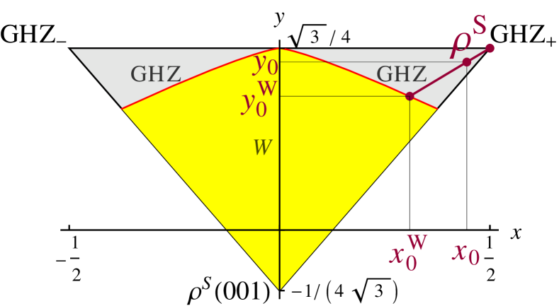
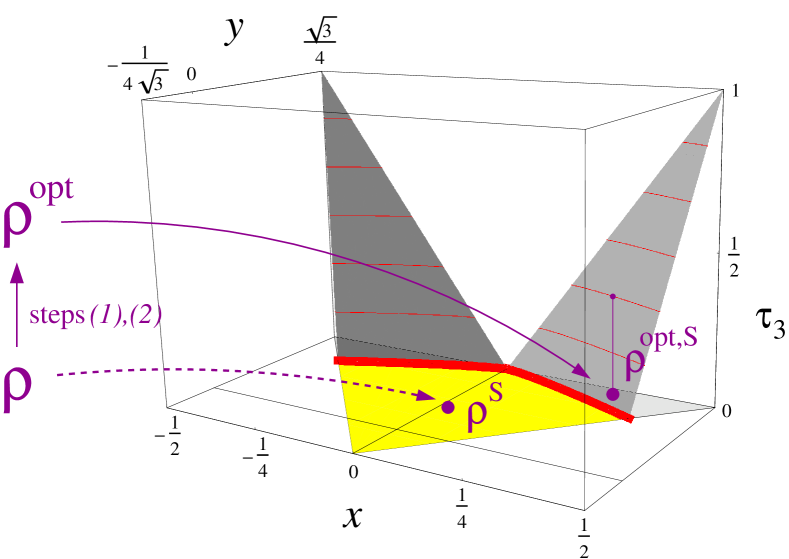
The GHZ-class entanglement of three-qubit states is quantified by the three-tangle (Refs. CKW2000 ; Viehmann2012APB , see also Methods). For GHZ-symmetric three-qubit states the exact solution for the three-tangle Siewert2012 (see also Methods) is
| (6) |
where and are the coordinates of the intersection of the GHZ/ line with the direction that contains both GHZ+ and (cf. Fig. 1). The grey surfaces in Fig. 2 illustrate this solution.
Now we turn to constructing a quantitative witness for the three-tangle of arbitrary three-qubit states by using the solution in equation (6). As before, the main idea is that an arbitrary state can be symmetrized according to equation (2) and thus is projected into the GHZ-symmetric states. Again, we assume real and nonnegative, so that . From Figs. 1 and 2 it appears evident that the entanglement of the symmetrization image can be improved by moving its point closer to GHZ+. More precisely, the entanglement measure is enhanced upon increasing one of the coordinates without decreasing the other (cf. equations (3) and (6)).
In this spirit, finding the normal form in step (1) is appropriate as it yields the largest possible three-tangle for a state locally equivalent to the original (cf. Ref. Verstraete2003 ). As the normal form is unique only up to local unitaries it does not automatically give the state with minimum entanglement loss in the symmetrization. Therefore, the unitary optimisation step (2) is required to generate the best coordinates.
In the symmetrization the information contained in various matrix elements is lost. For two qubits, however, the concurrence of the optimised Bell-diagonal states depends only on and the loss of in the symmetrization does not harm. In contrast, the three-qubit normal form depends on about 45 parameters. We may not expect that depends only on two of them and, hence, entanglement loss in the symmetrization (3) is inevitable (cf. Supplementary Information). Consequently, steps (1)-(3) lead to a lower bound for the three-tangle that coincides with the exact at least for those states which are locally equivalent to a GHZ-symmetric state. The most straightforward optimisation criterion in step (2) is to maximise . Alternative criteria which generally do not give the best but can be handled more easily (possibly analytically) are maximum fidelity , minimum Hilbert-Schmidt distance of from GHZ+, or maximum .
II Discussion
Evidently this approach can be generalised. Therefore we conclude with a discussion of some of its universal features. The essential ingredients are an exact solution of the entanglement measure for a sufficiently general family of states with suitable symmetry, and the entanglement optimisation for a given arbitrary state via general local operations. The former determines the border where the entanglement vanishes. The latter ensures an appropriate fidelity of the image with the maximally entangled state. This reveals a remarkable relation between entanglement quantification through SL invariants and the standard entanglement witnesses which we briefly explain in the following.
A well-known witness for two-qubit entanglement is . It detects the entanglement of an arbitrary normalised two-qubit state if
On the other hand, from our concurrence result
| (7) | ||||
we see, by dropping the optimisation over SLOCC , that is a (non-optimised) quantitative witness for two-qubit entanglement. In other words, yields one of the many possible lower bounds to the exact result. Analogously it is straightforward to establish the relation between the standard GHZ witness and the non-optimal quantitative witness . The latter represents a linear lower bound to the three-tangle obtained via the optimisation steps (1)–(3) (see Supplementary Information).
Finally we mention that our approach can be used without optimisation, i.e., either without step (1), or (2), or both. This renders the witness less reliable but more efficient. At best it requires only four matrix elements (for any ). We note that, if we apply the witness to a tomography outcome the measurement effort can be reduced by using the prior knowledge of the state and choosing the local measurement directions such that the fidelity with the expected GHZ state is measured directly. This implements optimisation step (2) right in the measurement.
III Methods
III.1 Normal form of an -qubit state
The normal form of a multipartite quantum state is a fundamental concept that was introduced by Verstraete et al. Verstraete2003 It applies to arbitrary (finite-dimensional) multi-qudit states. Here we focus on -qubit states only.
In the normal form of an -qubit state , all local density matrices are proportional to the identity. Therefore the normal form is unique up to local unitaries. Remarkably, the normal form can be obtained by applying an appropriate local filtering operation
where . Therefore is locally equivalent to the original state . The normal form is peculiar since it has the minimal norm of all states in the orbit of generated by local filtering operations. Practically, the normal form can be found by a simple iteration procedure described in Ref. Verstraete2003 It is worth noticing that GHZ-symmetric states – which play a central role in our discussion – are naturally given in their normal form.
III.2 Three-tangle of three-qubit GHZ-symmetric states
The pure-state entanglement monotone that needs to be considered for three-qubit states is the three-tangle , i.e., the square root of the residual tangle introduced by Coffman et al. CKW2000 :
| (8) |
Here with are the components of a pure three-qubit state in the computational basis. The three-tangle becomes an entanglement measure also for mixed states via the convex-roof extension Uhlmann1998
| (9) |
i.e., the minimum average three-tangle taken over all possible pure-state decompositions . In general it is difficult to carry out the minimisation procedure in equation (9). For GHZ-symmetric three-qubit states, however, the convex roof of the three-tangle can be calculated exactly (see equation (6)). This solution is shown in Fig. 2 and can be understood as follows. The border between the and the GHZ states is the GHZ/ line which has the parametrised form Eltschka2012
| (10) |
with . The solution for the convex roof is obtained by connecting each point of the GHZ/ line with the closest of the points . That is, the three-tangle is nothing but a linear interpolation between the points of the border between GHZ and states, and the maximally entangled states GHZ±.
References
- (1)
references
Acknowledgements
This work was funded by the German Research Foundation within SPP 1386 (C.E.), and by Basque Government grant IT-472-10 (J.S.). The authors thank R. Fazio, P. Hyllus, K.F. Renk, and A. Uhlmann for comments, and J. Fabian and K. Richter for their support.
SUPPLEMENTARY INFORMATION
for
“A quantitative witness for Greenberger-Horne-Zeilinger entanglement”
by Christopher Eltschka and Jens Siewert
III.1 Two-qubit GHZ-symmetric states
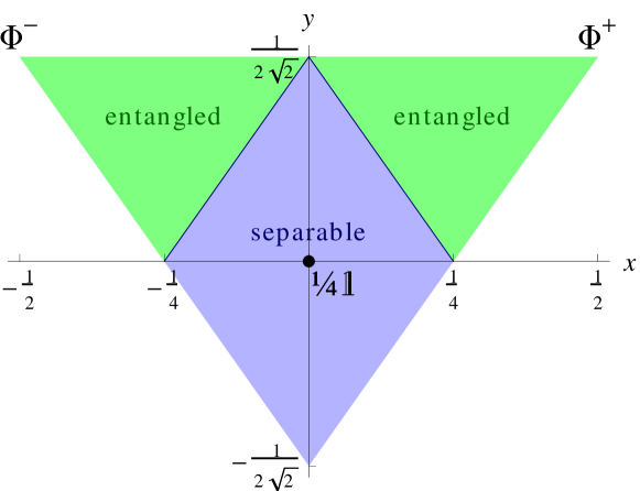
The twirling operation equation (2) in the main text defines a family of GHZ-symmetric mixed states for each qubit number . The simplest case is that of two qubits. The symmetrization of an arbitrary two-qubit state is characterised by two real parameters for which we choose the following parametrization Siewert2012
| (S1) | |||||
| (S2) |
We emphasise that these coordinates (as well as those in equations (4), (5) in the main text) are defined for normalised density matrices. The corresponding states form a triangle in the plane, see Supplementary Fig. S1.
The entanglement monotone considered here is the concurrence . Its convex-roof extension Uhlmann1998 is defined in analogy with equation (9) in the main text via
| (S3) |
i.e., the average concurrence minimised over all possible pure-state decompositions of the two-qubit state . The concurrence of GHZ-symmetric two-qubit states is a function of the coordinates Siewert2012
| (S4) |
We can rewrite this formula in terms of the matrix elements of the original state using equations (S1), (S2), keeping in mind that symmetrization cannot increase the concurrence:
| (S5) |
i.e., we obtain equation (3) of the main text. The analogy with some of the equations in Ref. Reimpell2007 is remarkable, in particular with equation (6), if we use as the only witness (with the optimal slope and the offset ). It arises due to the fact that the concurrence of GHZ-symmetric two-qubit states is a linear function, and the linear one-witness approximation in Ref. Reimpell2007 becomes exact. We note also that our concurrence formula in the main text, , is reminiscent of the so-called fully entangled fraction Bennett1996 . However, the optimisation of the fully entangled fraction includes only local unitaries while our approach allows for general SLOCC operations.
III.2 Normal form of two-qubit states
According to Verstraete et al. it is always possible to obtain a Bell-diagonal (renormalised) normal form for two-qubit states Verstraete2003 ; Verstraete2001 . That is, can be written as a mixture
where , and is a permutation of the four Bell states . Evidently the Bell-diagonal form with maximum is one where and . It is not difficult to see that by applying appropriate combinations of the local operations , , , as well as
to the qubits in , it is always possible to achieve the correct permutation of the Leinaas2006 . Note that this implies that there cannot be another Bell-diagonal normal form derived from the original two-qubit state with a concurrence larger than that of .
Bennett et al. have demonstrated that the concurrence of a Bell-diagonal two-qubit density matrix depends only on its largest eigenvalue Bennett1996 . Therefore can be determined exactly without reference to the Wootters-Uhlmann method Wootters1998 ; Uhlmann2000 and does not change on applying the symmetrization operation equation (2) in the main text.
We mention that in the two-qubit case the different optimisation criteria for step (2) (i.e., maximal concurrence of , maximal fidelity with , maximal , and minimal Hilbert-Schmidt distance from ) are equivalent.
III.3 Entanglement loss in three-qubit symmetrization
In the main text we have mentioned that for three qubits one may not expect to find the exact three-tangle for arbitrary mixed states, and that in general entanglement is lost in the symmetrization. This statement is illustrated by the mixtures
versus
where , . It is known Eltschka2008 ; Jung2009 that has non-vanishing three-tangle for , as opposed to which is GHZ-entangled only for . Note that is already given in the normal form. For the normal form can be calculated analytically.
In the range the exact three-tangle of is Viehmann2012APB while . The optimisation leaves and practically unchanged. The corresponding points in the plane are located close to each other and still in the region of states, i.e., we obtain the estimates . Hence, the GHZ entanglement in will be underrated while that of is determined exactly.
III.4 Relation between projective GHZ witness and quantitative witness
In the discussion part of the main text we mention that the standard projective GHZ witness can, in modified form, be used as a quantitative witness. Here we explain this fact in more detail.
The standard witness detects the GHZ-type entanglement in an arbitrary three-qubit state : it is a GHZ-class state if . Our aim is to elucidate that is a quantitative witness for , i.e., that
| (S6) |
is a lower bound to for arbitrary three-qubit states .
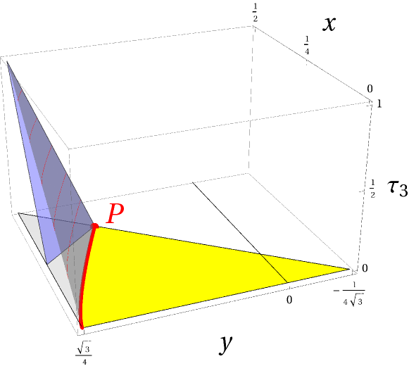
It appears obvious that, in order to obtain a non-optimal witness, it is not necessary to use the GHZ/ line which is difficult to handle analytically. The solution of the two-qubit case suggests the following simpler alternative: We start at the end point of the GHZ/ line and consider the straight line which contains this point and is parallel to the lower-left border of the triangle. Its equation is . It crosses the triangle only in the GHZ part, that is, its points lie above the GHZ/ line. For all the states which correspond to triangle points on this line the Hilbert-Schmidt scalar product with GHZ+ equals .
From Supplementary Fig. S2 it is easy to see that a plane which contains this line and the point represents a lower bound to the three-tangle of GHZ-symmetric three-qubit states. It is straightforward to check that the function corresponding to the points of that plane is given by
| (S7) |
As the plane lies below the exact we have also
Further, the operator has GHZ symmetry so that for an arbitrary state
By combining the preceding relations and the conclusions from the Section “Results” in the main text we obtain
| (S8) |
which confirms the desired result, equation (S6). We mention that also here there is a certain freedom whether or not one wants to optimise the state before symmetrizing it. One may note the relation between this type of equation deriving from our method and some of the findings in Sections 3.4–3.6 of Ref. Eisert2007 , as well as those in Ref. LS2012
From these remarks one might feel tempted to conclude that our method is a mere extension to the standard witness approach as it detects GHZ entanglement in a given state more or less according to the fidelity of the GHZ state and assigns a number to it. To clarify this point consider the example
The exact three-tangle is , that is, the state contains GHZ entanglement for arbitrarily small . While the standard witness would not detect entanglement for our approach produces the correct value (with a relative error ) for values as small as .