The HST eXtreme Deep Field XDF:
Combining all ACS and WFC3/IR Data on the HUDF Region into the Deepest Field Ever

Abstract

The eXtreme Deep Field (XDF) combines data from ten years of observations with the HST Advanced Camera for Surveys (ACS) and the Wide-Field Camera 3 Infra-Red (WFC3/IR) into the deepest image of the sky ever in the optical/near-IR. Since the initial observations on the Hubble Ultra-Deep Field (HUDF) in 2003, numerous surveys and programs, including supernova followup, HUDF09, CANDELS, and HUDF12 have contributed additional imaging data across this region. Yet these have never been combined and made available as one complete ultra-deep image dataset. We do so now with the eXtreme Deep Field (XDF) program. Our new and improved processing techniques provide higher quality reductions of the total dataset. All WFC3/IR and optical ACS data sets have been fully combined and accurately matched, resulting in the deepest imaging ever taken at these wavelengths ranging from 29.1 to 30.3 AB mag ($5\sigma$ in a $0.35^{\prime\prime}$ diameter aperture) in 9 filters. The combined image therefore reaches to 31.2 AB mag $5\sigma$ (32.9 at $1\sigma$) for a flat $f_{\nu}$ source. The gains in the optical for the 4 filters done in the original ACS HUDF correspond to a typical improvement of 0.15 mag, with gains of 0.25 mag in the deepest areas. Such gains are equivalent to adding $\sim$130 to $\sim$240 orbits of ACS data to the HUDF. Improved processing alone results in a typical gain of $\sim$0.1 mag. Our $5\sigma$ (optical+near-IR) SExtractor catalogs reveal about 14140 sources in the full field and about 7121 galaxies in the deepest part of the XDF.

1. Introduction

Since the first Hubble Deep Field was observed in 1995 (Williams et al., 1996), the Hubble Space Telescope has demonstrated its ability to probe ever deeper limits as new capabilities are added. The combination of deeper images and new cameras with sensitivity at redder wavelengths has pushed the redshift limits well into the reionization epoch in the first Gyr of the universe.

The Hubble UltraDeep Field (HUDF; Beckwith et al., 2006) was observed in 2003 with the then-new Hubble Advanced Camera (ACS) that had been placed into Hubble in 2002 by the Shuttle astronauts during the servicing mission SM3B. ACS provided over an order of magnitude gain in discovery efficiency (the product of survey area and efficiency) over the WFPC2 and an added redder filter (F850LP) that opened up the universe at $z\sim 5-6$ (e.g. Bouwens et al., 2004a; Bunker et al., 2004; Yan & Windhorst, 2004).

The ACS HUDF was released as a public image in 2004. The HUDF, along with the companion wide-field GOODS images (Giavalisco et al., 2004), revealed large numbers of $z\sim 6$ galaxies (Bouwens et al., 2006; Bouwens et al., 2007) at the end of the reionization epoch for the first time. The NICMOS near-IR camera provided the first glimpse of galaxies at $z\sim 7$ (Bouwens et al., 2004b; Yan & Windhorst, 2004), just 800 Myr after the Big Bang (Thompson et al., 2005), but it was not until the new infrared Wide Field Camera 3 (WFC3/IR) was added to Hubble in 2009 by the Shuttle astronauts in the final Hubble servicing mission (SM4) that the reionization epoch was opened up to extensive exploration (e.g. Oesch et al., 2010; Bouwens et al., 2010; McLure et al., 2010; Bunker et al., 2010; Finkelstein et al., 2010). The remarkable gain in discovery efficiency (over 40$\times$ for WFC3/IR compared to NICMOS) hinted at the gains to be seen when JWST becomes operational.

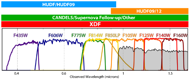
Figure 1.— The XDF input datasets and spectral elements. The XDF combines all the data that have been taken on the HUDF field between 2002 and 2013 - this means HUDF, HUDF09, CANDELS, HUDF12 and many other programs. No other release has done this. This makes the deepest image from HST ever, with the widest spectral coverage image from HST on the HUDF. An example galaxy spectrum at $z=6.5$ is shown. This example galaxy is seen about 12.8 billion years ago, just 800 million years after the Big Bang. Due to the high fraction of neutral hydrogen present at this early cosmic time, the source is essentially completely invisible at optical wavelengths probed by the ACS camera and it can only be seen in the near-infrared with the new WFC3/IR. The wide wavelength coverage of the XDF images allow for the identification of similar galaxies across a very large redshift range, from $z\sim 4$ to $z\sim 12$.

Table 1XDF Summary

Position (J2000)	R.A. 03h 32m 38.5s, Dec. $-$27∘ 47′ 00″
Area (XDF total)	10.8 arcmin2
Area (XDF deep IR)	4.7 arcmin2
Instruments	ACS/WFC and WFC3/IR
Exposure Dates	July 2002 to December 2012
Total Exposure Time	21.7 days ($\sim$2 million seconds)
Number of Exposures	2963 (1972 ACS/WFC; 991 WFC3/IR)
Typical Depths	$\sim$30 AB mag ($5\sigma$) in most filters
Combined Depth	31.2 AB mag ($5\sigma$) for a flat $f_{\nu}$ source
Archive Link	http://archive.stsci.edu/prepds/xdf/

Note. — Depths are for $5\sigma$ detections measured in circular apertures of 0$\farcs$35 diameter and are not corrected to total magnitudes.

The HUDF was observed as part of the HUDF09 program in 2009 (PI: Illingworth; e.g. Bouwens et al., 2011b) as one of the first set of images taken by the new infrared camera of WFC3. These first observations in mid-2009 were combined and released as the HUDF09 image in early 2010. The HUDF09 observations were finally completed in the spring of 2011. Thanks to the ultra-deep coverage in the near-infrared, these data allowed for the first systematic exploration of galaxies at $z\sim 10$, resulting in the identification of then the most distant, earliest galaxy candidate ever seen, UDFj-39546284 (Bouwens et al., 2011a; Oesch et al., 2012).

The next step in the exploration was with the CANDELS program (PI:Faber/Ferguson; Grogin et al., 2011; Koekemoer et al., 2011) that played a role akin to GOODS but now with the WFC3/IR camera, providing wide-field data that improved the statistics at higher luminosities. These data are an invaluable resource and contribute to the HUDF region, but the most important addition in the near-IR was from the HUDF12 (PI:Ellis; Ellis et al., 2013) dataset which provided additional near-IR data from WFC3/IR over the HUDF09 field. This dataset provided comparable data to the HUDF09 program in some of the same filters, as well as observations using the F140W filter. Together the HUDF09, CANDELS and HUDF12 datasets provide near-IR depths over part of the HUDF area that are roughly comparable (AB mag) to that from the original ACS dataset.

Such deep imaging in several filters across the optical to the near-infrared is required to identify and study galaxies in the early universe from $z\sim 4$ out to $z\sim 10$. Such galaxies can be selected quite robustly due to the strong inter-galactic absorption from neutral hydrogen (e.g. Madau, 1995). The wavelength coverage and filter curves of the HST dataset over the HUDF, along with an example SED for a high redshift galaxy, is shown in Figure 1.

The concept of the eXtreme Deep Field (XDF) resulted from the realization in late 2011 that all the data taken over the last ten years with the Advanced Camera and the Wide Field Camera 3 on the Hubble UltraDeep Field had not been combined into a single extremely deep image. The HUDF, HUDF09, CANDELS and numerous other datasets had been released individually, but a combined image of all the images ever taken on the HUDF had not been done.

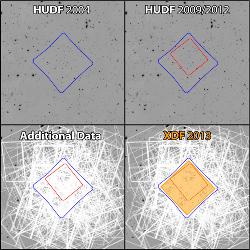
Figure 2.— The steps involved in building up the eXtreme Deep Field (XDF). The first image (top left) of the sequence shows the original HUDF data from the ACS. By fraction of total exposure time the original HUDF contributes over 50% to the XDF, but only contains data in the optical region of the spectrum in four filters. In 2009, the HUDF09 project took images towards the red end of the spectrum in the near-infrared with the new WFC3/IR camera. These new data doubled the waveband coverage and enabled exploration for high redshift galaxies in the reionization epoch for the first time. The second image (top right) of the sequence adds the HUDF09 field with WFC3/IR that contributed around a 20% of the data (by exposure time) to the XDF. Finally, the XDF/HUDF09 team took all the other data on this region taken by numerous programs and combined it through a very laborious series of steps into the incredibly deep XDF image. As the third image (bottom left) shows, the data fall at many locations and orientations and much careful checking was needed to make sure all the Hubble ACS and WFC3/IR images were properly aligned and combined. The contributions came from seventeen other programs that comprised about 30% of the time, of which the largest were the CANDELS dataset from ACS and WFC3/IR and the HUDF12 WFC3/IR dataset. The various supernova followup programs also made substantial contributions. Finally, in the fourth image (bottom right) of the sequence the XDF is shown as the orange region where the contribution of every image over the last decade from ACS and WFC3 has been included.

With the release of the HUDF12 observations at the end of its proprietary period in Dec 2012 the full data set was available from the nineteen Hubble programs that had taken observations in this region over the past decade. This data set was dominated by the original HUDF, the HUDF09 and the more recent HUDF12 data, but with important and significant contributions from many other programs, including various supernovae followup programs and CANDELS (see Section 2 and Table 2). In this paper, we describe how all these datasets were combined to make the deepest image of the sky ever. The broad process of building up the XDF is shown schematically in Figure 2.

The XDF will remain the deepest image ever taken, with only marginal future gains practical, until JWST flies. And even then, while JWST will push to fainter limits at $\lambda\gtrsim 0.7\mu$m, the shorter wavelength datasets (F435W and probably F606W) will remain unique until a new telescope flies that has blue optical imaging capabilities.

This paper is structured as follows: Section 2 describes the observations that contribute to the XDF, Section 3 describes the data processing in some detail for the ACS datasets and the WFC3/IR datasets, while Section 3.5 summarizes the data products that have been supplied for community use to the Mikulski Archive for Space Telescopes (MAST). The tests on the datasets to verify their veracity are given in Section 4, and a summary is provided in Section 5.

2. The Observations

2.1. ACS/WFC and WFC3/IR Data over the XDF

Here we briefly discuss the HST observations that were used to create the XDF dataset. In its current form the XDF includes over 10 years of ACS/WFC and 3 years of WFC3/IR observations taken from mid-2002 through the end of 2012. These observations include data from the original ACS optical HUDF program (HST PID 9978) and the WFC3/IR HUDF09 and HUDF12 programs (HST PID 11563 and 12498). A complete list of HST programs that contribute to the XDF dataset is given in Table 2.

Table 2HST programs contributing to the XDF

Program ID	HST Cycle	Program Title
9352	11	The Deceleration Test from Treasury Type Ia Supernovae at Redshifts 1.2 to 1.6
9425	11	The Great Observatories Origins Deep Survey: Imaging with ACS (GOODS)
9488	11	Cosmic Shear - with ACS Pure Parallel Observations
9575	11	ACS Default (Archival) Pure Parallel Program
9793	12	The Grism-ACS Program for Extragalactic Science (GRAPES)
9978	12	The Ultra Deep Field with ACS (HUDF)
10086	12	The Ultra Deep Field with ACS (HUDF)
10189	13	Probing Acceleration Now with Supernovae (PANS)
10258	13	Tracing the Emergence of the Hubble Sequence Among the Most Luminous and Massive Galaxies
10340	13	Probing Acceleration Now with Supernovae (PANS)
10530	14	Probing Evolution And Reionization Spectroscopically (PEARS)
11359	17	Panchromatic WFC3 survey of galaxies at intermediate z: Early Release Science program for Wide Field
		Camera 3 (ERS)
11563	17	Galaxies at $z\sim 7-10$ in the Reionization Epoch: Luminosity Functions to $<$0.2L* from Deep IR Imaging of
		the HUDF and HUDF05 Fields (HUDF09)
12060	18	Cosmic Assembly Near-IR Deep Extragalactic Legacy Survey — GOODS-South Field, Non-SNe-Searched
		Visits (CANDELS)
12061	18	Cosmic Assembly Near-IR Deep Extragalactic Legacy Survey — GOODS-South Field, Early Visits of SNe
		Search (CANDELS)
12062	18	Galaxy Assembly and the Evolution of Structure over the First Third of Cosmic Time - III (CANDELS)
12099	18	Supernova Follow-up for MCT (CANDELS)
12177	18	3D-HST: A Spectroscopic Galaxy Evolution Treasury (3DHST)
12498	19	Did Galaxies Reionize the Universe? (HUDF12)

In order to specifically determine which HST observations to include in the XDF dataset we executed searches using the MAST HST archive. We constrained our search to include only HST ACS/WFC and WFC3/IR imaging observations within a 13 arc-minute radius of the original HUDF coordinates ($\alpha=$ 03:32:39.0, $\delta=$ $-$27:47:29.0) while limiting the search to the HST filters F435W, F606W, F775W, F814W, F850LP, F105W, F125W, F140W, F160W, and the exposure time to $>100$ seconds. Although, there have been many other HST observations taken with legacy instruments (e.g WFPC2 and NICMOS) we chose to use only imaging data from HST’s current optical and near-IR instruments and only filters where a substantial investment of HST orbits had been contributed. Once we had determined the set of observations to include in the XDF dataset, we used the HST MAST archive or the Canadian Astronomy Data Centre (CADC) HST archive to acquire these data.

Our search resulted in a total of 2963 $HST$ exposures, 1972 in the optical filters of ACS/WFC and 991 exposures in the NIR with WFC3/IR. These images sum up to a total exposure time of almost 2Ms. This corresponds to about 21.7 days of actual open-shutter observing time (13.6 days in ACS and 8.1 days in WFC3/IR). To acquire this amount of data would have taken $HST$ about 790 orbits or about 52 days of clock time.

As would be expected from looking at the distribution of exposures in Figure 2, the exposure times vary significantly across the image for the different filters. The total exposure times per filter are shown in Table 3, while exposure time maps per filter are presented in Figures 3 and 5.

Table 3XDF exposures

Filter	Exposure Time (ks)	# of Exposures
ACS/WFC
F435W	152.4	164
F606W	174.4	286
F775W	377.8	460
F814W	50.8	362
F850LP	421.6	700
ACS Total	1177.0	1972
WFC3/IR
F105W	266.7	248
F125W	112.5	289
F140W	86.7	118
F160W	236.1	336
WFC3 Total	702.0	991

3. Data Calibration and Reduction

In this section we describe the data reduction process for both the ACS/WFC and WFC3/IR images, and how we aligned these images to the original HUDF data.

Our processing begins by visually inspecting all images included in the XDF dataset in order to identify any data quality issues. This includes problems due to loss of guiding, excessive background or pointing inaccuracies. During the visual inspection we also identify images affected by satellite trials and optical ghosts from filter reflections generated by bright stars (in ACS/WFC) and updated the data quality array to ensure that these artifacts are masked during processing. Any image for which a data quality issue could not be corrected was rejected from the dataset and not processed.

The development of procedures that handled large numbers of images with arbitrary centering and orientation was very challenging. Key issues that had to be dealt with included ensuring that the distortion solutions were correct, that the information used for alignment was correct, that cosmic rays were handled appropriately so as to ensure that compact sources were not clipped but the overall CR removal was optimized, and that background variations were minimized. Combining all these data into a common dataset, and ensuring that all the data were well-aligned, cleaned of cosmic rays and artifacts, and were photometrically reliable, was a time-consuming task that took considerable effort from its inception early in 2012 until submission to MAST in 2013.

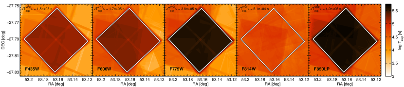
Figure 3.— Exposure time maps of the XDF images in the five ACS filters. The central diamond shape pointings are from the original HUDF program (Beckwith et al. 2006), which took data in all filters except F814W. The median exposure time over the HUDF area is indicated on the top, ranging from $\sim 5\times 10^{4}$ s in F814W to $\sim 4\times 10^{5}$ s in F850LP. The wider area data around the original HUDF imaging have been taken mostly as part of the original GOODS program, and for F814W from CANDELS. In addition, a multitude of follow-up programs over the last 10 years have added to this larger area dataset. The white outline shows the boundary of the released XDF image to the MAST archive.

3.1. Pre-processing ACS/WFC images

The ACS/WFC channel consists of two $4096\times 2048$ pixel detectors at a scale of $~{}0\farcs 05$ pixel^-1 providing a $~{}202^{\prime\prime}\times 202^{\prime\prime}$ field of view. All ACS/WFC images used in the XDF dataset were processed through the most recent version of the ACS calibration pipeline calacs (2012.2). The standard calibration process includes bias subtraction, dark current correction, bad pixel masking and flat-fielding. In addition to these calibration processes, images taken after HST Servicing Mission 4 (SM4), have been corrected for Charge Transfer Efficiency (CTE) degradation (Anderson & Bedin 2010), bias shift, bias striping (Grogin et al. 2011), and amplifier crosstalk (Suchkov et al. 2010).

3.2. ACS/WFC image reduction process

The XDF ACS/WFC dataset was processed by the data reduction pipeline APSIS (Blakeslee, et al. 2003). The reduction process is quite similar to the process used by the MultiDrizzle software package (Koekemoer et al. 2002) where each image is passed through a full drizzle-blot-drizzle cycle. Images are background subtracted and drizzled onto a common tangential-plane pixel grid. These images are median stacked and the median stack image is blotted back to each input image position and used as a template for cosmic-ray rejection. A cosmic-ray mask is generated for each image and combined with the data quality array. The final image mosaic is produced by drizzling all the input images onto a single image mosaic and combining them with inverse-variance weight maps that take into account all noise sources (readout, dark current and background noise).

While APSIS is perfectly adequate for producing science quality images when combining datasets consisting of tens of images, the XDF dataset, with hundreds of images, required further processing.

3.2.1 ACS/WFC image registration

Since the pointing accuracy of HST is only good to within a few arc-seconds, the WCS of each image must be refined in order to acquire precise registration across all images within the ACS/WFC dataset. APSIS performs the image registration process using software we developed called superalign (see Appendix A). Briefly, superalign takes as input, both source positions from a reference catalog and source positions from catalogs generated for each image (after rectifying each catalog to remove the geometric distortion). superalign then uses these positions to compute accurate shift and rotation corrections that are applied to each input image. The input reference catalog was generated from an image produced by combining the original HUDF F775W image with an astrometrically calibrated GOODS mosaic to provide accurate alignment both over and outside the HUDF area.

To optimize alignment within the ACS/WFC dataset we split the images into two groups: a deep group with images from the original HUDF observations that are observed at a single position and two orientations, and a shallow group, made up of the remaining images, which are observed at a large variety of positions and orientations. These two groups are processed separately with superalign while using the same input reference catalog. The frame-by-frame alignment within our dataset is excellent as shown in Figure 4.

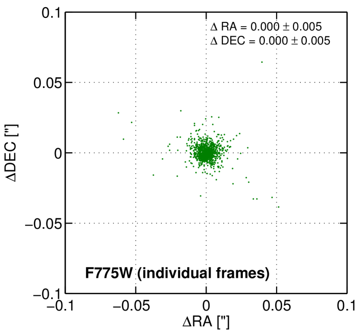
Figure 4.— Relative alignment of individual frames of the XDF F775W data. The plot shows the offsets of five galaxies and stars in the individual images relative to the position of these sources in the final XDF image. There are 1972 individual frames in the final optical XDF image. This figure shows that the individual frames align to much better than a single original ACS pixel (0$\farcs$05). The standard deviation in RA and DEC offsets are reported on the upper right of the plot, indicating that individual frames are aligned to within 1/10 of a pixel.

3.2.2 ACS/WFC final mosaics

To create the ACS/WFC mosaics we process the dataset for each filter through the APSIS pipeline in three passes. The purpose of the first two passes are to remove any excess background emission on individual exposures. This background emission only becomes evident when stacking a large number of overlapping exposures. Starting with the standard calibrated images (flt or flc files) acquired from the HST archive as input, we create super-median stacked images for each detector and each filter in the first pass. The median images are created by halting the pipeline processing after the blotting process and using the individual blotted images to aggressively mask sources when combining the stacked super-median images. These are subsequently subtracted from the individual images. This process is repeated in the second pass, but this time using the subtracted images from the first pass as input and relaxing the masking threshold. Again, these super-median images are subtracted from the individual input images, which are then used in the final pass where the full pipeline is run to create the final image mosaics. These are created with multidrizzle and combine all the input images with the use of inverse-variance weight maps.

Given the large number of input images used in each filter we elected to use the “point” kernel and a pixfrac of 0 in the final drizzling process. In making use of this pixfrac, we remain consistent with the original 2004 release by Beckwith et al. (2006) who use the same pixfrac.

As expected it was not a simple or quick process to generate the final XDF mosaic. Processing the full ACS/WFC dataset through our pipeline involved processing 1.1 terabytes and took 10 days, and so each processing iteration was a lengthy effort. As problems were found, the origin of the problems needed to be identified, a fix made, and the full dataset processed again. Iterating to a final version suitable for a MAST release required many months of effort.

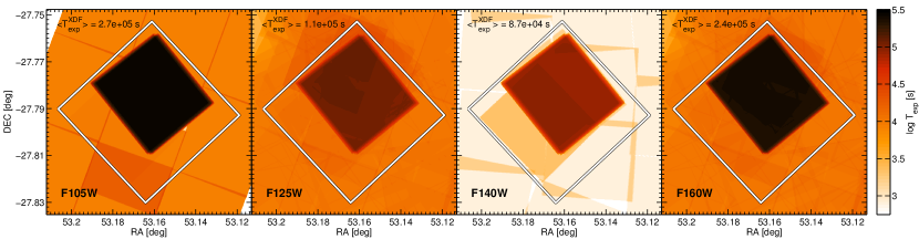
Figure 5.— Exposure time maps of the XDF images in the four WFC3/IR filters. The vast majority of images in these filters comes from a WFC3/IR pointing position that was common to both the HUDF09 and HUDF12 programs. The median exposure time in the deepest part is indicated on the top. The colorbar indicates the range of exposure times. The total exposures range from $\sim 9\times 10^{4}$ s to $\sim 3\times 10^{5}$ s. The wider area data have been taken mostly as part of the CANDELS Deep program.

3.3. Pre-processing WFC3/IR images

Our basic processing of the WFC3/IR images is based on the calwf3 pipeline as outlined below.

The WFC3 IR channel uses a $1024\times 1024$ pixel detector with the outer 5 pixels on each side of the detector containing reference bias pixels yielding a final $1014\times 1014$ px image at a scale of $~{}0\farcs 135\times 0\farcs 121$ pixel^-1 and a $~{}131^{\prime\prime}\times 121^{\prime\prime}$ field of view. All WFC/IR images are obtained in MULTIACCUM mode in which each image contains two short bias readouts followed by a number of non-destructive readouts as determined by the NSAMP parameter set in the Phase II proposal.

The standard calwf3 processing of a WFC3/IR image includes initializing the data quality array and flagging known bad pixels, subtracting the mean bias level computed from reference pixels surrounding the detector for each readout and then subtracting the zeroth (bias) read from each readout in order to remove any signal from external sources. It then proceeds by correcting for the non-linear detector response, subtracting the appropriate dark current reference image in each readout, computing photometric header keywords and converting the units of the science and error data arrays to a count rate. This is followed by an “up-the-ramp” fitting in order to combine the data from each readout while identifying and flagging pixels suspected of cosmic-ray hits. The final step in the processing corrects for pixel-to-pixel and large scale variations across the detector by dividing by the appropriate flat field image and then multiplying by the gain of the detector so the final units will be in electrons per seconds. This step produces the final calibrated image with the flt name extension.

3.3.1 Variable background correction

While most WFC3/IR flt files produced by calwf3 can be used without further calibration, in some cases calwf3 can falsely flag a large fraction pixels as cosmic-rays. For WFC3/IR MULTIACCUM mode observations, calwf3 assumes that accumulating background counts over the entire observation are linearly increasing. This assumption may not be the true for all observations, in particular, if the background varies across an exposure. This can cause calwf3 to reject a significant fraction of the accumulated pixel fluxes, effectively resulting in a shorter exposure time in affected pixels. The TIME array extension of the flt files can thus be used to determine whether non-linearities in the background count rate are a problem.

We tested different criteria, and found that problematic frames can be identified by an average exposure time of the TIME array that varies by more than 2% from the header EXPTIME value. For such images, we introduce one additional step to the calwf3 processing.

We begin by acquiring the raw image and running the calwf3 tasks DQICORR, ZSIGCORR, BLEVCORR, ZOFFCORR, NLINCORR, DARKCORR, and FLATCORR. We then halt the processing and scale the sky background in each of the individual MULTIACCUM readout science arrays to match the average sky count rate across the exposure. This additional processing step ensures the background count rate to be linear, before processing the image with the calwf3 cosmic-ray rejection task CRCORR. After background subtraction, the processing is concluded by running the calwf3 task CRCORR, UNITCOR and PHOTCORR, generating a new cosmic-ray corrected calibrated flt image.

3.3.2 WFC3/IR Persistence masking

The WFC3/IR detector can exhibit ghost sources from bright objects imaged in earlier exposures due to persistence. For the XDF WFC3/IR dataset we therefore excluded all pixels that are significantly affected by source persistence. To determine which pixels to exclude we utilized the persistence models generated by the STScI WFC3 Persistence Project. The project generates a persistence model for each WFC3/IR exposure based on the time history of previous exposures, incorporating internal persistence (from exposures within a visit) and external persistence (from exposures from earlier visits). These are combined to create a model of the total (internal plus external) persistence flux per pixel.

We tested different masking criteria, and we found that excluding all pixels with model persistence flux of 0.2 electrons/s and growing this mask by 2 pixels, results in clean images that are not significantly affected by source persistence.

3.4. WFC3/IR image reduction process

The XDF WFC3/IR dataset was processed using tasks provided in the data reduction pipeline WFC3RED. For a general description of the WFC3RED pipeline see Magee, Bouwens & Illingworth 2011. The WFC3RED pipeline takes as input the pre-processed WFC3/IR flt images and an external reference image used for registration and performs background subtraction, image registration, creation of inverse variance weight-maps (for drizzling) and generation of the final distortion-free image mosaics.

The background in WFC3/IR images can vary dramatically from image to image depending on the observational conditions and can contain features on various scales. The WFC3RED pipeline preforms background subtraction by utilizing a two-pass background model. In each pass, a median filter is applied to the image and subtracted after aggressively masking sources. In the first pass a large grid size (165 pixels) is used in order to remove any large scale gradients. In the second, a smaller grid size (39 pixels) is used to remove smaller scale background features. In order to improve the pixel-by-pixel S/N, and correct for any imperfections in the flats or darks, WFC3RED median stacks all the background subtracted images in each filter in the dataset to create super-median background images. These are subsequently subtracted from the individual images.

WFC3RED performs the image registration process in two steps. The first registration step is preformed by superalign. While superalign accurately determines the shift and rotation correction to be applied to most of the WFC3/IR images we find that for some images a small correction is needed.

As a second registration step, WFC3RED therefore uses MultiDrizzle to create distortion-free image stacks for each visit in the dataset and then cross-correlates the sources in each image stack with sources in the external reference image. Minor corrections to the shift and rotation are then applied to the WCS of each image in the visit to obtain an optimal registration.

Specifically, for the alignment of the XDF dataset, we used the original HUDF F775W image for registration, combined with astrometrically calibrated GOODS mosaics, to provide accurate alignment outside of the HUDF area. Thanks to our two step alignment procedure, the registration of the $XDF$ image to the HUDF is better than 1/10 of a pixel (i.e., $<0\farcs 003$; see section 4.2).

WFC3RED creates the final image mosaics for each filter by running MultiDrizzle in three passes. For the first pass, each filter dataset is processed using the full drizzle-blot-drizzle cycle. Each individual image is drizzled to a separate undistorted image matching the same size, scale and orientation as the external reference image (i.e., the HUDF image in the case of the XDF). These images are then stacked into a single image using the MultiDrizzle “median” algorithm. The stacked median image is then blotted back to each of the input image (distorted) positions, rescaled by the exposure time, and used as a clean template for identifying cosmic-rays and bad pixels. A cosmic-ray/bad-pixel mask is created and the data quality array is updated for each image. Lastly, a combined drizzle image is produced for each filter by using the inverse variance weight maps.

In order to remove any excess background emission in the final image mosaics, WFC3RED runs MultiDrizzle a second time. In this pass only the blotting back process of MultiDrizzle is run, but this time using a combined drizzle image from the first pass to create an image at each position. These images are then used to create a median stack of images in each filter – but now masking out the sources apparent in the combined drizzle image (rather than just those apparent in the individual images). These super-median images are subtracted from each of the individual images.

In the last pass only, the final image combination step of MultiDrizzle is run. A final image mosaic is created for each filter, using inverse variance weight-maps with a pixfrac of 0.8, a “square” kernel, and an output scale of $0\farcs 06$ pixel^-1.

The WFC3/IR dataset involved a slightly smaller but still comparable effort to that involved in processing the ACS/WFC dataset. Nearly 1000 exposures totaling $\sim 0.7$ million seconds in the 4 wide WFC3/IR filters were processed to form the extremely deep near-infrared dataset for the XDF. The two primary components to the WFC3/IR data were from the HUDF09 and the HUDF12 programs, but with additional contributions from the CDF-S CANDELS dataset.

While the two primary datasets were closely aligned, the CANDELS data was at different orientations and centers and added to the complexity of the task for the WFC3/IR data. Processing the WFC3/IR data has many challenges similar to those of the ACS, but the WFC3/IR data also bring some unique challenges to the table. The issues that required particular attention were the mis-flagging of pixels as cosmic rays, persistence effects and dealing with dramatically varying backgrounds. Fortunately the smaller WFC3/IR datasets ($\sim 300$ Gbyte) processed more rapidly (typically within a day) and so it was possible to evaluate the output of a processing run, derive a fix for a problem and do another run with a reasonable turnaround of several days. Nonetheless, the total time to identify the data problems, refine the software, test and fully process the data, and iterate as needed, meant that the WFC3/IR data also took many months of effort.

Table 4XDF Image Depths

Filter	$5\sigma$ Depth	$5\sigma$ Depth
	Aperture	Total
ACS/WFC
F435W	29.8	29.6
F606W	30.3	30.1
F775W	30.3	30.1
F814W	29.1	28.9
F850LP	29.4	29.2
WFC3/IR
F105W	30.1	29.7
F125W	29.8	29.4
F140W	29.8	29.3
F160W	29.8	29.3
Combined for flat $f_{\nu}$ Source
ACS	30.8	30.6
ACS+WFC3	31.2	30.9

Note. — Depths are measured in circular apertures of 0$\farcs$35 diameter on the 60 mas XDF images over the part where the WFC3/IR data are deepest (see Figure 5). The corrections to total magnitudes (last column) are based on the encircled energy tabulated in the ACS and WFC3/IR handbooks.

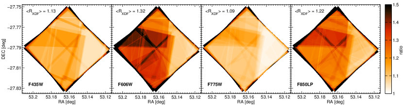
Figure 6.— Gain in exposure time of the XDF images compared to the original HUDF data. The largest gains are obtained in F606W and F850LP. The largest gains from additional data in the follow-up programs were taken in these filters. The gain scale is shown at the right. The largest contribution of additional data came from our HUDF09 program, which added ACS parallel data that covers the left $\sim 75\%$ of the XDF image. The median exposure time gains over the XDF image are indicated in the upper left corner of each panel.

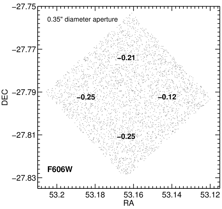
Figure 7.— Gains in 5$\sigma$ depth of the XDF image compared to the original HUDF image in the F606W filter. The small dots correspond to empty sky positions which were used to measure the flux fluctuations in small circular apertures of 0$\farcs$35 diameter. The gains in depth vary between 0.12 mag to 0.25 mag across the image due to the varying gains in exposure time. The average gain in F606W is 0.18 mag. These gains are somewhat larger than expected purely based on the added exposure time. In particular, our subtraction of a sky image results in markedly smoother background than achieved in the original HUDF images leading to a gain in depth of about 0.1 mag just from the improved background.

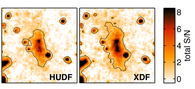
Figure 8.— Images of signal-to-noise (not intensity) comparing the improvement of S/N in the combined ACS optical data set for a small 2$\farcs$5 region around a low-surface brightness galaxy in the HUDF/XDF. The pixel-by-pixel S/N was computed for a pixel size of 0$\farcs$09 in the total stacked ACS data which included all images in the F435W, F606W, F775W, and F850LP filters. This is shown for the HUDF on the left and for the XDF on the right at the same color stretch, as indicated by the colorbar on the right that shows the corresponding S/N. The black contours indicate where the S/N is larger than 1.5. Clearly, both the lower surface brightness parts and the core of this galaxy are detected more significantly in the new XDF image.

3.5. Data Products

The XDF data products are organized into sets of images by passband (ACS/WFC F435W, F606W, F775W, F814W & F850LP; WFC3/IR F105W, F125W, F140W & F160W) and image scale. We drizzled the data to two different scales 0.06^′′/pixel and 0.03^′′/pixel. The ACS benefits from drizzling to a 0.03^′′/pixel scale because of its smaller native pixels and the better point-spread function (PSF) at shorter wavelengths, and so we provide the ACS data at this scale. These 30mas images are exactly aligned with the original HUDF ACS images, having the same pixel positions and WCS configuration.

For the WFC3/IR data, a 0.06^′′/pixel scale is more appropriate. We provide matched ACS and WFC3/IR data at the 60 mas scale. Each 60 milli-arcsecond/pixel image is approximately 5k $\times$ 5k pixels and each 30 milli-arcsecond/pixel image is approximately 10k $\times$ 10k pixels. For each filter we provide both the science and inverse variance weight image.

The full set of XDF data products are available through the MAST High Level Science Products (HLSP) archive at http://archive.stsci.edu/prepds/xdf/.

Table 5$5\sigma$ Depths of XDF compared to HUDF ACS images

Filter	XDF Depth	XDF Range	HUDF Depth
F435W	29.72	29.69 - 29.79	29.60
F606W	30.20	30.14 - 30.27	30.02
F775W	30.26	30.23 - 30.31	30.10
F850LP	29.43	29.41 - 29.46	29.23

Note. — The limits correspond to $5\sigma$ variations in the sky flux measured in a circular aperture of 0$\farcs$35 diameter on the 30 mas XDF ACS images.

4. XDF Characteristics and Gains

In the following sections, we present some of the characteristics of the XDF images and compare them to the original HUDF ACS images (Beckwith et al., 2006) as well as the previous release of the WFC3/IR data over the HUDF as part of the HUDF12 program (Ellis et al., 2013; Koekemoer et al., 2012).

4.1. Improvement in Depth Relative to HUDF Images

In Figure 6, we show the gains in exposure time of the XDF image relative to the original HUDF ACS images. Since many of the additional data were taken as parallel images (mostly as part of the HUDF09 program), the added exposure time is highly position dependent. In particular, the HUDF09 parallel ACS observations do not cover the whole XDF image, resulting in maximal gains in exposure time over the eastern part of the image (left on the figures), and only small increase in exposure time on the west (right).

In order to quantify the (position-dependent) gain in the depth of the images, we selected 5000 random empty sky regions of the images and measured the flux variation in circular apertures of 0$\farcs$35 diameter. This was done both in the XDF and in the original HUDF images. The flux variations are converted into 5$\sigma$ magnitude depths and are reported in Table 5. As can be seen, averaged over the whole field, the XDF images are $0.12-0.20$ mag deeper than the original HUDF data.

We quantify the depth variations around the field seen in Figure 6 in Figure 7 for one of the ACS filters, F606W. As expected, the eastern part of the image (left) shows much greater gains in depth than is average for the image. Due to the increases in exposure time, the eastern part is deeper by 0.25 mag in that filter compared to the HUDF image.

While these gains may seem small (0.12 mag to 0.25 mag), it is worthwhile considering that to achieve these gains through a new imaging program would require between 100 to 240 orbits of new data, and so the effort expended on maximizing the return from existing datasets results in valuable and very cost-effective gains.

Note that the minimum gains are actually quite significant, averaging about 0.1 mag, even in the parts of the images which only got a very small increment in exposure time. The minimum gain in the redder filters is quite substantial, reaching 0.13 mag and 0.18 mag, while in the bluer filters it is 0.09 mag and 0.12 mag. This is mainly due to our subtraction of a sky image, which results in markedly smoother background compared to the original processing of the HUDF dataset. It is clear from the original HUDF images that the background is smoother in the bluer filters than it is in the redder filters and this is reflected in the gains that we see from the improved processing.

To exemplify the gains made, we provide a direct comparison in Figure 8 between the original HUDF and the XDF of a galaxy with low surface brightness structure.

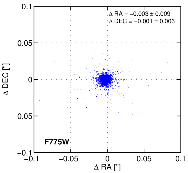
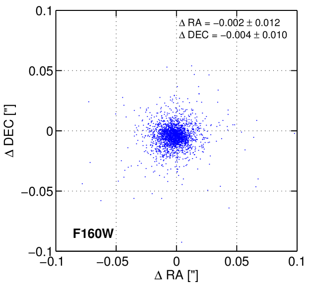
Figure 9.— Top – Alignment of the XDF F775W data relative to the original HUDF images. The plot shows $\sim 3500$ galaxies indicating that the alignment is better than 1/10 pixel (or $<$3 mas at our px scale of 30mas). The median offsets and the standard deviation in RA and DEC are reported on the upper right of the plot. Bottom – Alignment of the XDF F160W image relative to the HUDF12 image release. Given the 60mas pixel scale of the WFC3/IR data, the alignment is again better than 1/10 pixel, or $<4$mas.

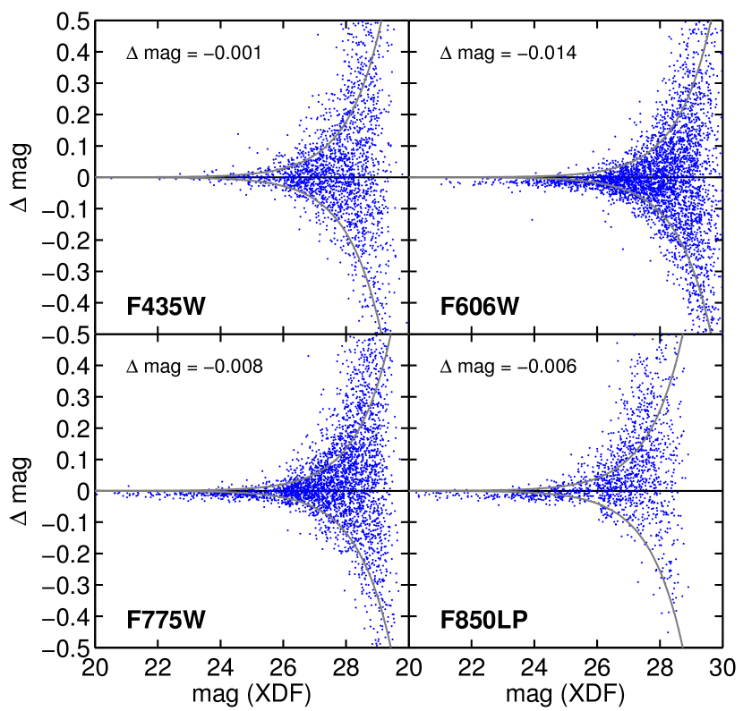
Figure 10.— XDF aperture photometry compared to the original HUDF data from identical sources in the optical images. Each panel shows a different filter image. Fluxes were measured in circular apertures of 1″diameter. The photometry is consistent at the 1% level. The gray lines show the expected scatter given the image depth in each filter.

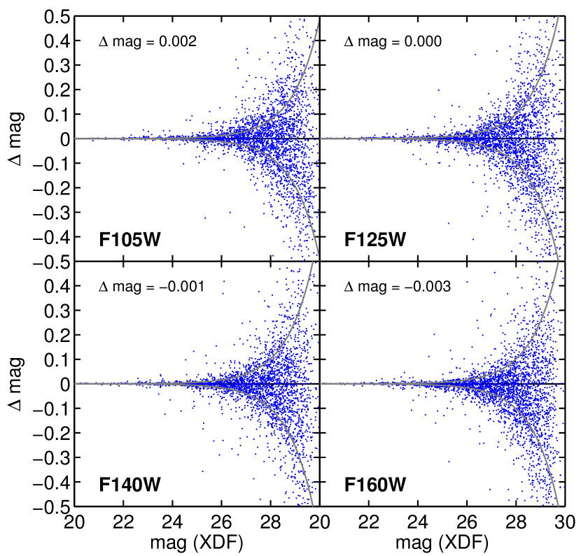
Figure 11.— Comparison of the XDF WFC3/IR photometry with the HUDF12 image release. Each panel shows the magnitude differences of about 3000 sources measured in circular apertures of 1″diameter. The XDF photometry is consistent with the HUDF12 image release at much better than 1%. The same is true when the XDF photometry is compared to the original HUDF09 image over the HUDF. The gray lines show the expected scatter given the magnitude limits in the same apertures.

4.2. Consistency with Previous HUDF ACS Images

One important test when creating a new image of the HUDF is consistency with the previous data. We therefore created independent catalogs of both datasets for a detailed comparison. In particular, we used the publicly available images of the HUDF from MAST.

The weight maps provided by multidrizzle are inverse variance maps. In order to use these as weight maps for source detection with SExtractor (Bertin & Arnouts, 1996), we converted these images to RMS maps using

$$\mathrm{RMS}=1/\sqrt{\mathrm{WHT}}$$

All pixels where $\mathrm{WHT}=0$ are set to 1 in the RMS-map.

We then run SExtractor (v2.8.6) to detect sources and measure their positions (X/Y_IMAGE) and fluxes in circular apertures (MAG_APER) of 0$\farcs$35 diameter. The source positions are compared in Figure 9, where we show that the alignment is better than 1/10 pixel. The median offsets are $<3$ milli-arcsec, with a standard deviation of 10 milli-arcsec.

In Figure 10, we compare the F775W photometry in circular apertures between the XDF and the HUDF images (using identical magnitude zeropoints). The photometry is very consistent, being $\lesssim 1\%$ in all cases except one. The only filter where the flux differences are larger than 1% is the F606W image. The exposure time gain in this filter is highest, and it is likely that the small changes in the ACS AB-magnitude zeropoint with time affect this filter most. In our reduction, we have not accounted for such drifts in the zeropoints over the last 10 years. If photometry to within better than 1% is required, this change must be accounted for. We plan to correct for this effect in a future release of the XDF images.

4.3. Consistency with Previous HUDF12 WFC3/IR Images

There have been two previous releases of WFC3/IR images over the HUDF field. In particular, after the completion of the HUDF09 program (PI: Illingworth), our team released a reduction to MAST including the full two years worth of data totalling 111 orbits of WFC3/IR imaging in the three filters F105W, F125W and F160W used in the HUDF09 observations.

Since then, another 128 orbits of WFC3/IR imaging were taken as part of the HUDF12 program (PI: Ellis). These images included additional F140W imaging and significantly increased the depth in the F105W filter image. A combination of WFC3/IR data from the HUDF09 and HUDF12 programs has been released to MAST by the HUDF12 team. The XDF image release includes our own reduction of these data together with all additional WFC3/IR data that have been taken over this field, and we drizzled these to an identical frame as the ACS imaging data for easy multi-wavelength analyses.

As we show in Figures 9 and 11, the WFC3/IR images of the XDF are in excellent agreement with the HUDF12 (and also the HUDF09) image release, both in terms of photometry and source positions. Aperture fluxes agree to within $<0.3\%$, and the alignment of these 60 mas images is again better than 1/10 pixel ($<4$ mas).

4.4. Number of Sources in the XDF

The total number of sources in a field, or equivalently, the surface density of sources, has routinely been used as a gauge to quantify how faint a field reaches. The original Hubble Deep Field North (Williams et al., 1996) revealed some $\sim$2000-3000 sources within a small 5.7 arcmin² area (depending on whether the catalog was based on the $V_{606}$-band image alone or the $V_{606}+I_{814}$ image). The Hubble Ultra Deep Field in 2004 (Beckwith et al., 2006) significantly extended the depth available over the HDF-North, famously finding some 10,144 sources in a $\sim$11 arcmin² area or $2\times$ the number of sources per unit area as was revealed in the original Hubble Deep Field North image.

With the availability of our even deeper XDF exposure over the HUDF region, we can revisit this question of source counts and the surface density of sources on the sky to very faint limits. Weighting the individual images according to the inverse-variance assuming a flat $f_{\nu}$ spectrum for sources, we constructed catalogs for the XDF using first only the optical ACS data over the $\sim$11 arcmin² full area with the HUDF region and second using the optical+near-IR data over the $\sim$4.7 arcmin² footprint originally defined by the HUDF09 program (see outlines in Figures 3 and 5).

Over the full $\sim$11 arcmin² area which made up the original HUDF release, our SExtractor catalogs reveal some 14140 sources on the coadded $B_{435}+V_{606}+i_{775}+I_{814}+z_{850}$ image with a S/N$>5$ (Kron [1980] apertures, with Kron parameters of 1.6 and 2.5). The smaller $\sim 4.7$ arcmin² area over which ultra-deep WFC3/IR imaging is available contains about 7121 galaxies above the same $5\sigma$ significance level, using as the detection image the coadded $B_{435}+V_{606}+i_{775}+I_{814}+z_{850}+Y_{105}+J_{125}+JH_{140}+H_{160}$ image.

The gains in depth in the optical lead to an $\sim 40$% increase in the total number of sources over the $\sim 11$ arcmin² HUDF area –- and an equivalent increase in the source surface density. Over the HUDF09 area where ultra-deep near-IR imaging data are available, we achieve even greater $\geq$50% gains in source surface density, as one might expect given the much greater depth of the collective optical+near-IR data set.

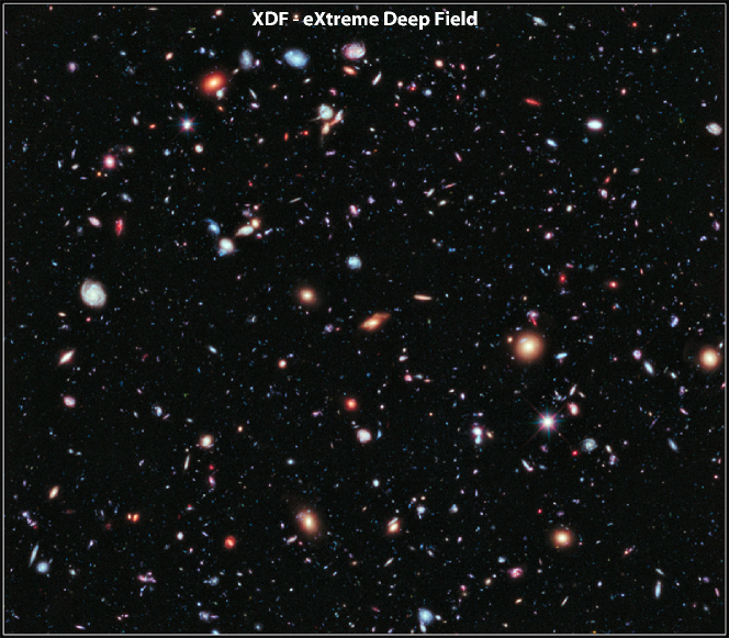
Figure 12.— A color image of the deepest region of the XDF, including both the ACS and WFC3/IR data. The ten years of data on the HUDF region from these cameras have led to the deepest image ever taken in the optical/near-IR. The point source $5\sigma$ depth in a 0$\farcs$35 diameter aperture in each filter is typically $\sim$30 AB mag, and is always deeper than 29 AB mag (see Table 4). The combined depth is $\sim$31.2 AB mag. High resolution versions of this figure can be found at http://xdf.ucolick.org/xdf.html.

5. Summary

In 2003 the data HUDF demonstrated the ability of HST and its new ACS camera to reach beyond 29 AB mag and to push the redshift limit for galaxies to $z\sim 6$ around 950 Myr after the Big Bang (e.g. Bouwens et al., 2004a; Bunker et al., 2004; Yan & Windhorst, 2004). Images with the resurrected NICMOS camera over part of the HUDF showed the potential of near-IR observations with HST for reaching to even earlier times, $z\sim 7$, just 800 Myr after the Big Bang (Bouwens et al., 2004b; Yan & Windhorst, 2004), but it was not until the advent of WFC3/IR in 2009 that this potential was fully realized. Images taken as part of the HUDF09 program with WFC3/IR reached out to $z\sim 10$ (Bouwens et al 2011, but see Ellis et al 2013, Bouwens et al 2013 and Brammer et al 2013 for further interesting developments from the HUDF12 dataset). While the data from these major programs constituted the most extensive programs on the HUDF, numerous other programs were adding to the available dataset on the HUDF, but until now, these datasets were not being used to enhance the HUDF.

The realization in late 2011 that the ten years of observations on the HUDF from 2002 to 2012 from numerous programs would allow us to push deeper over the HUDF region led to a program to combine all images from the ACS and the WFC3/IR into the deepest optical/IR image ever. The dataset from combining all the available data would provide a resource for numerous programs on distant galaxies, and would complement the extensive wide-field, but shallower datasets now available like CANDELS and GOODS.

The goal of the program we undertook was to combine all available ACS and WFC3/IR data over the HUDF region into a co-aligned dataset that would result in the deepest ever image. The resulting dataset was named the eXtreme Deep Field (XDF) to highlight the substantial improvements from taking all the available data. The deepest part of the XDF image, in the region selected initially for the HUDF09 WFC3/IR data, is shown as a color image in Figure 12.

The development of procedures that handled large numbers of images with arbitrary centering and orientation was very challenging. Key issues that had to be dealt with included ensuring that the distortion solutions were correct, that the information used for alignment was correct, that cosmic rays were handled appropriately so as to ensure that compact images were not clipped but the overall cosmic-ray removal was optimized, and that background variations were minimized. Combining all these data into a common dataset, and ensuring that all the data were well-aligned, cleaned of cosmic rays and artifacts, and were photometrically reliable, was a time-consuming task that took considerable effort from its inception early in 2012 until submission to MAST in 2013.

The key steps to realizing the XDF were:

• Nearly 2000 exposures of ACS data totalling $\sim$1.2 million seconds in 5 wide filters were processed to provide the extremely deep optical dataset for the XDF. The original HUDF data in 4 filters dominated the ACS contribution but a large number of additional exposures with arbitrary centering and orientation from a further 15 HST programs were also incorporated. These data included large numbers of exposures with partial overlap.

• The resulting ACS image for the XDF added depth through both additional data and also through improved processing. Much has been learnt about the ACS data since 2003. The reprocessing of all the data from the HUDF and the other 15 programs enabled us to deal with some issues that particularly affected the background (e.g., post SM4 striping and CTE correction). As a result of the new processing approaches and the overall reprocessing the new dataset has smoother backgrounds. This provides a typical depth gain of about 0.1 mag. While small, this is equivalent to adding about 100 orbits of data with the ACS, so the improvement is an important addition to the HUDF dataset. The actual depth gains around the ACS field varied from about 0.1 mag to 0.25 mag, corresponding to adding about 100-240 orbits of data to the original HUDF.

• The XDF ACS data, for a point source in a $0.35^{\prime\prime}$ diameter aperture, reaches to $5\sigma$ AB mag depths of 29.8 (F435W), 30.3 (F606W, F775W), 29.1 (F814W) and 29.4 (F850LP). The total flux from a point source is 0.2 mag brighter (i.e., subtract 0.2 mag to give $5\sigma$ AB mag $total$ flux depths). The ACS dataset has a combined depth for a flat $f_{\nu}$ source of 30.8 AB mag $5\sigma$ in a $0.35^{\prime\prime}$ diameter aperture.

• The WFC3/IR data for a point source in a $0.35^{\prime\prime}$ diameter aperture, reaches to $5\sigma$ AB mag depths of 30.1 (F105W) and 29.8 (F125W, F140W, F160W). The $5\sigma$ AB mag depths are $\sim$0.4 mag brighter for the $total$ flux from a point source. The WFC3/IR and ACS dataset together, in the deepest part of the XDF image, has a combined depth for a flat $f_{\nu}$ source of 31.2 AB mag $5\sigma$ in a $0.35^{\prime\prime}$ diameter aperture.

• The processed datasets, ACS and WFC3/IR, were submitted to MAST and made publicly available on April 5, 2013 (http://archive.stsci.edu/prepds/xdf/). They consist of co-aligned images at 60 mas for both WFC3/IR and the ACS, and a separate set just for the ACS at 30 mas (since the ACS data has higher resolution intrinsically). Both the XDF ACS and XDF WFC3/IR images are aligned with the original HUDF within a few mas, or less than $1/{10}$ px.

• The WFC3/IR photometry matches within 0.000-0.003 mag (mean difference $0.002$ mag) of the HUDF12 release (Koekemoer et al 2013) with a $1^{\prime\prime}$ diameter aperture. The fluxes are also very similar at smaller aperture sizes, being 4% larger in the XDF images. This indicates that the PSF in the new reduction is slightly tighter than the HUDF12 reduction.

• Photometry on the XDF matches the original HUDF within 0.001-0.014 mag (mean difference $0.007$ mag). The differences are small, but measurable and are thought to reflect some aspect of the changing zero points with time for the ACS data (resulting from ACS detector temperature changes). While very small, we plan to resolve any remaining zeropoint uncertainties for a future release.

The remarkable depth of the XDF is unlikely to be exceeded until JWST is launched, and even then it will not be exceeded in the blue (F435W), and possibly not even in the green region of the optical spectrum (F606W), until a new space telescope with optical capability is launched. The XDF will remain a cornerstone of the CDF-S and will remain the deepest image of the sky for a long time to come. It will be a centerpiece for a wide range of studies at high redshift for faint galaxies at redshifts around $z\sim 2$ out to the limit of Hubble at $z\sim 11$.

Appendix A SuperAlign

A.1. Overview

superalign is a short C code we (RJB) developed to determine the internal shifts and rotations for an arbitrary number of (overlapping) contiguous images from a set of (distortion free) catalogs. It requires good initial guesses for the shifts and rotations (within 2.5 arcsec and 0.5 degrees of the true solution, respectively), and thus is ideal for use with HST data where these quantities are only approximately known. This code was originally developed for use with the ACS GTO pipeline APSIS and offers several useful advantages relative to other image registration packages:

1. It does not require that all images be contiguous with a single reference image. This allows one to construct arbitrarily large mosaics out of individual images.

2. Input catalogs can include substantial ($>80\%$) contamination from cosmic rays.

A.2. Algorithm

The algorithm that superalign uses to align large sets of exposures has a tree-like structure:

1. First, superalign groups the exposures in terms of those that substantially overlap.

2. Second, group by group (pointing by pointing), superalign iteratively aligns all the exposures. As it finds alignments that work between exposures within a group, it constructs an increasingly complete list of the probable stars. Candidate stars which appear in a statistically significant number of exposures are added to the complete list, while candidate stars which do not are classified as CRs.

3. After generating a complete list of all the stars from each group, superalign begins building up a mosaic of stars starting at the central group and iteratively accreting nearby groups (to produce an ever larger list of stars). As each group is accreted, the relative position/rotation of all the groups added up to that point (within the ever growing mosaic) is re-optimized to minimize the overall error.

superalign uses a variation on the similar triangle method (Groth 1986) to determine the alignment between two individual catalogs. However, instead of attempting to find similar triangles in both images, superalign looks for similar bi-directional vectors (object pairs with the same separation and the same relative orientation). After finding similar vectors, superalign uses these vectors to determine a candidate transformation from one catalog onto another. Each transformation is given a score based upon how well it maps objects from one catalog onto the other. The transformation with the highest score is then adopted as the starting point in one final refinement step, where we perturb the coefficients in this transformation using a Markov Chain Monte Carlo process in an attempt to further improve the accuracy of the alignment.

References

- Anderson & Bedin (2010) Anderson, J., & Bedin, L. R. 2010, PASP, 122, 1035
- Beckwith et al. (2006) Beckwith, S. V. W., Stiavelli, M., Koekemoer, A. M., et al. 2006, AJ, 132, 1729
- Bertin & Arnouts (1996) Bertin, E., & Arnouts, S. 1996, A&AS, 117, 393
- Blakeslee et al. (2003) Blakeslee, J. P., Anderson, K. R., Meurer, G. R., Benítez, N., & Magee, D. 2003, Astronomical Data Analysis Software and Systems XII, 295, 257
- Bouwens et al. (2004a) Bouwens, R. J., Illingworth, G. D., Blakeslee, J. P., Broadhurst, T. J., & Franx, M. 2004a, ApJ, 611, L1
- Bouwens et al. (2004b) Bouwens, R. J., Thompson, R. I., Illingworth, G. D., et al. 2004b, ApJ, 616, L79
- Bouwens et al. (2006) Bouwens, R. J., Illingworth, G. D., Blakeslee, J. P., & Franx, M. 2006, ApJ, 653, 53
- Bouwens et al. (2007) Bouwens, R. J., Illingworth, G. D., Franx, M., & Ford, H. 2007, ApJ, 670, 928
- Bouwens et al. (2010) Bouwens, R. J., Illingworth, G. D., Oesch, P. A., et al. 2010, ApJ, 709, L133
- Bouwens et al. (2011a) Bouwens, R. J., Illingworth, G. D., Labbe, I., et al. 2011a, Nature, 469, 504
- Bouwens et al. (2011b) Bouwens, R. J., Illingworth, G. D., Oesch, P. A., et al. 2011b, ApJ, 737, 90
- Bouwens et al. (2013) Bouwens, R. J., Oesch, P. A., Illingworth, G. D., et al. 2013, ApJ, 765, L16
- Brammer et al. (2013) Brammer, G. B., van Dokkum, P. G., Illingworth, G. D., et al. 2013, ApJ, 765, L2
- Bunker et al. (2004) Bunker, A. J., Stanway, E. R., Ellis, R. S., & McMahon, R. G. 2004, MNRAS, 355, 374
- Bunker et al. (2010) Bunker, A. J., Wilkins, S., Ellis, R. S., et al. 2010, MNRAS, 409, 855
- Ellis et al. (2013) Ellis, R. S., McLure, R. J., Dunlop, J. S., et al. 2013, ApJ, 763, L7
- Finkelstein et al. (2010) Finkelstein, S. L., Papovich, C., Giavalisco, M., et al. 2010, ApJ, 719, 1250
- Giavalisco et al. (2004) Giavalisco, M., Dickinson, M., Ferguson, H. C., et al. 2004, ApJ, 600, L103
- Grogin et al. (2010) Grogin, N. A., Lim, P. L., Maybhate, A., Hook, R. N., & Loose, M. 2010, in 2010 Space Telescope Science Institute Calibration Workshop - Hubble after SM4. Preparing JWST, ed. S. Deustua and Cristina Oliveira (Baltimore: STScI)
- Grogin et al. (2011) Grogin, N. A., Kocevski, D. D., Faber, S. M., et al. 2011, ApJS, 197, 35
- Groth (1986) Groth, E. J. 1986, AJ, 91, 1244
- Koekemoer et al. (2003) Koekemoer, A. M., Fruchter, A. S., Hook, R. N., & Hack, W. 2003, HST Calibration Workshop : Hubble after the Installation of the ACS and the NICMOS Cooling System, 337
- Koekemoer et al. (2011) Koekemoer, A. M., Faber, S. M., Ferguson, H. C., et al. 2011, ApJS, 197, 36
- Koekemoer et al. (2012) Koekemoer, A. M., Ellis, R. S, McLure, R. J., et al. 2012, arXiv:1212.1448
- Kron (1980) Kron, R. G. 1980, ApJS, 43, 305
- Madau (1995) Madau, P. 1995, ApJ, 441, 18
- Magee et al. (2011) Magee, D. K., Bouwens, R. J., & Illingworth, G. D. 2011, Astronomical Data Analysis Software and Systems XX, 442, 395
- McLure et al. (2010) McLure, R. J., Dunlop, J. S., Cirasuolo, M., et al. 2010, MNRAS, 403, 960
- Oesch et al. (2007) Oesch, P. A., Stiavelli, M., Carollo, C. M., et al. 2007, ApJ, 671, 1212
- Oesch et al. (2010) Oesch, P. A., Bouwens, R. J., Illingworth, G. D., et al. 2010, ApJ, 709, L16
- Oesch et al. (2012) Oesch, P. A., Bouwens, R. J., Illingworth, G. D., et al. 2012, ApJ, 745, 110
- Oke & Gunn (1983) Oke, J. B., & Gunn, J. E. 1983, ApJ, 266, 713
- Suchkov et al. (2010) Suchkov, A. A., Grogin, N. A., Sirianni, M., et al. 2010, in 2010 Space Telescope Science Institute Calibration Workshop - Hubble after SM4. Preparing JWST, ed. S. Deustua and Cristina Oliveira (Baltimore: STScI)
- Szalay et al. (1999) Szalay, A. S., Connolly, A. J., & Szokoly, G. P. 1999, AJ, 117, 68
- Thompson et al. (2005) Thompson, R. I., Illingworth, G., Bouwens, R., et al. 2005, AJ, 130, 1
- Williams et al. (1996) Williams, R. E., Blacker, B., Dickinson, M., et al. 1996, AJ, 112, 1335
- Yan & Windhorst (2004) Yan, H., & Windhorst, R. A. 2004, ApJ, 612, L93