Physics of a partially ionized gas relevant to galaxy formation simulations – the ionization potential energy reservoir

Abstract

Simulation codes for galaxy formation and evolution take on board as many physical processes as possible beyond the standard gravitational and hydrodynamical physics. Most of this extra physics takes place below the resolution level of the simulations and is added in a “sub-grid” fashion. However, these sub-grid processes affect the macroscopic hydrodynamical properties of the gas and thus couple to the “on-grid” physics that is explicitly integrated during the simulation.

In this paper, we focus on the link between partial ionization and the hydrodynamical equations. We show that the energy stored in ions and free electrons constitutes a potential energy term which breaks the linear dependence of the internal energy on temperature. Correctly taking into account ionization hence requires modifying both the equation of state and the energy-temperature relation. We implemented these changes in the cosmological simulation code Gadget2.

As an example of the effects of these changes, we study the propagation of Sedov-Taylor shock waves through an ionizing medium. This serves as a proxy for the absorption of supernova feedback energy by the interstellar medium. Depending on the density and temperature of the surrounding gas, we find that up to 50% of the feedback energy is spent ionizing the gas rather than heating it. Thus, it can be expected that properly taking into account ionization effects in galaxy evolution simulations will drastically reduce the effects of thermal feedback. To the best of our knowledge, this potential energy term is not used in current simulations of galaxy formation and evolution.

1 Introduction

Even with the computing power currently available, it is still impossible to include all relevant physical processes in numerical simulations of galaxy formation and to explicitly solve all the relevant equations. Therefore, recourse is often taken to splitting the physics into a numerically manageable ‘macroscopic’ part, whose equations are integrated explicitly during a simulation, and a numerically intractable ‘microscopic’ part, whose equations are not solved explicitly (Springel, 2005; Teyssier, 2002; Springel, 2010). Out of necessity, these microscopic extensions usually offer a phenomenological or heuristic description of much more complex physical processes. Examples are complex nuclear reaction networks (Pakmor et al., 2012) and radiative cooling and heating of a multi-phase, multi-component gas (Shen et al., 2010; Anninos et al., 1997). Clearly, it is mandatory for the assumptions underlying the microscopic physics to be compatible with those on which the macroscopic physics is based. A mismatch between the microscopic and macroscopic levels could hamper the reliability of numerical hydrodynamical simulations in a priori unknown ways.

In this paper, we focus on the connection between the microscopic and macroscopic physics in hydrodynamical simulations of an ionizing gas. Our main interest is the study of the low-density interstellar medium of galaxies, subject to heating by supernova explosions and the cosmic ultraviolet background. The lowest-order gas model is the so-called ideal gas. Extending on this, the use of more general equations of state is widespread in the literature. In Choi & Wiita (2010) a temperature-dependent treatment of the adiabatic index of a simple proton-electron plasma was proposed, while in Marek et al. (2009) a study of a mixture of baryonic gas and neutrinos was performed. Likewise, the energy equation has been adapted to different physical circumstances. For instance, a gas is heated when irradiated by ionizing UV radiation while recombination is a source of cooling due to the radiative loss of the kinetic energy of each captured electron (Mizuta et al., 2005).

However, because of the energy spent freeing an electron, each ion-electron pair constitutes a small amount of potential energy. Therefore, a partially ionized gas has an internal potential energy reservoir at its disposal that can absorb and release energy. In a gas composed of only Hydrogen and Helium and sufficiently dense to be in thermodynamic equilibrium, this potential energy reservoir can straightforwardly be taken into account using Saha’s equation to determine the ionization equilibrium and the Stefan-Boltzmann law to treat both cooling and heating (Stamatellos et al., 2007; Mihalas & Mihalas, 1984). This approximation is valid for circumstellar discs and star-forming molecular cores but it does not apply to a multi-component, optically thin gas such as the interstellar medium of galaxies. This requires a more rigorous numerical calculation of the ionization equilibrium and the corresponding potential energy stored in ions while also using a realistic treatment of gas cooling and heating.

The kinetic energy of the free electrons and the heating of gas, e.g. by ionizing radiation, have already been included in many state-of-the-art hydrodynamics codes, but this potential energy reservoir was to the best of our knowledge never before taken into account in cosmological or galaxy evolution simulations. In this paper, we show how this potential energy reservoir can be added to the microscopic physics of a numerical simulation and we investigate its effects.

2 Modified hydrodynamics

The internal energy of a partially ionized multi-component gas is given by

$$\rho u = \frac{3}{2}\left(\sum_{X}n_{X}+n_{e}(T)\right)kT$$ (1)

$$+\sum_{X}\left[\sum_{i}n_{X,i}(T)\left(\sum_{j=1}^{i}\varepsilon_{X,j}\right)\right].$$

Here, $n_{X,i}(T)$ is the number density of the $i^{\textrm{th}}$ ion of element $X$, $n_{e}$ is the free electron density, and $\varepsilon_{X,i}$ is the energy required to produce this ion by removing an electron from the $(i-1)^{\textrm{th}}$ ion, ground state to ground state. From charge conservation it follows that $n_{e}(T)=\sum_{i}i\,n_{X,i}(T)$. The second term in Eq. (1) gives the potential energy reservoir associated with the ionization. The temperature-dependent density of free electrons also affects the equation of state.

The system of hydrodynamical equations is closed by introducing an equation of state, which in this case reads

$$p=\left(\sum_{X}n_{X}+n_{e}(T)\right)kT=\frac{\rho kT}{\mu(T)},$$ (2)

and which is easily implemented by using a temperature-dependent mean particle mass $\mu(T)$. It is clear from these equations that the relation $p=(\gamma-1)\rho u$, which is generally used to simplify the hydrodynamical equations (Springel & Hernquist, 2002) no longer holds. This means that (a) the entropy based formulation of hydrodynamics is no longer possible and, (b) temperature becomes a hydrodynamical variable in the system and has to be integrated along with the equations of motion.

2.1 Energy-temperature dependence and the adiabatic index

We have numerically calculated and compiled the ionization equilibrium, and the cooling and heating rates of gases with a wide range of compositions, densities, temperatures, and heating sources (De Rijcke et al., 2013). For this work, we have extended the capabilities of ChiantiPy, a Python interface to the Chianti atomic database (Landi et al., 2012). For all ions, we use the recombination rates, collisional ionization rates, and energy level populations provided by ChiantiPy. Photo-ionization cross-sections are adopted from Verner et al. (1996) and integrated over the adopted stellar and cosmic UV- backgrounds in order to obtain the photo-heating and radiative cooling rates. The latter are required for the integration of the energy equation. With the ionization equilibrium in hand, we can evaluate Eq. (1) and infer the gas temperature from the internal energy. The temperature derivatives of Eq. (1) at constant density and at constant volume then yield the temperature dependent adiabatic index $\gamma(T)$ of the gas.

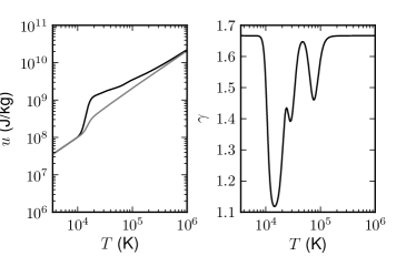
Figure 1: Specific internal energy (left) and adiabatic index $\gamma$ (right) as a function of temperature for a gas consisting of 92% H and 8% He. The gray line on the left plot traces the internal energy without taking into account the potential energy reservoir.

The adiabatic index and internal energy are plotted in Fig. 1 for of a gas consisting of 92% H and 8% He (by particle number), mimicking the unenriched interstellar medium. The transitions between the different ionization stages of H and He are clearly visible as steep drops of the adiabatic index. For comparison, we also plotted the internal energy without the potential energy reservoir (gray curve). Taking into account the potential energy reservoir associated with the ionization significantly alters the hydrodynamical properties of the gas; around 15,000 K, where $\gamma\sim 1.1$, the gas behaves almost isothermally: the ionizing hydrogen provides the gas with a large number of additional degrees of freedom. Heavier elements in the interstellar medium usually have abundances that are significantly smaller than those of H and He, and have a negligible impact on the adiabatic index. This was verified by calculating the adiabatic index with Chianti, both with and without metals present. Even for solar abundance ratios (Grevesse et al., 2010), both calculations yield almost identical results.

2.2 Excited states

So far, we assumed all ions to be in their ground states. For dense gases, this approximation can be invalid. It is straightforward to extend expression (1) by including a summation over each ion’s energy level occupations. This more general treatment can then be used to check if the approximation holds. For a given ion, excited states usually only become populated at temperatures where further ionization also gains importance and the ion’s density decreases steeply. Hence, their effect is completely dominated by the ionization effect. However, for elements like O and Fe having low-lying excited states, the picture is less straightforward. We calculated the adiabatic index, with and without taking into account excited states, and found essentially identical results, even for solar abundance ratios. Only for a pure O or Fe gas does the difference amount to a few percent at most. This justifies the use of this approximation.

3 Sedov-Taylor blast wave

The effect of our advanced treatment of ionization on the gas dynamics can be illustrated by means of a classical test case for hydrodynamical simulation codes: the Sedov-Taylor blast wave. The problem consists of a homogeneous gas cloud, in which a spherical shock wave propagates radially outward. For a gas with negligible internal energy and constant adiabatic index, the radius of the shock wave as a function of time is given by

$$r_{s}=\left(\frac{E_{0}}{\alpha(\gamma)\rho_{1}}\right)^{1/5}t^{2/5},$$ (3)

where $\alpha(\gamma)$ is a numerical factor which can be calculated by imposing energy conservation, $E_{0}$ is the total energy of the shock, and $\rho_{1}$ is the density of the ambient gas (Sedov, 1977). $\alpha$ is a monotonically decreasing function of $\gamma$, hence the shock wave propagates more slowly in a medium with smaller $\gamma$ or, equivalently, with more internal degrees of freedom per particle. If the gas has a non-negligible internal energy, the counter-pressure exerted by the ambient gas on the shock front must be taken into account. The analytical solution is then somewhat more involved but leads to the same conclusion: ionization is anticipated to slow down the propagation of expanding shock waves.

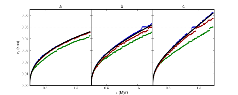
Figure 2: Shock wave radius as a function of time for a gas with a density of $\rho=81$ amu cm^-3 and an initial temperature (a) 100 K, (b) 5,000 K, and (c) 15,000 K. The gray dots (blue dots in the online version) represent the simulation values with the old gas physics, the black dots (green dots in the online version) are the values for the new gas physics, the full line is the analytical solution following Sedov (1977). The gray crosses (red dots in the online version) represent simulation values obtained by omitting the potential energy term, but with taking into account the change in particle number caused by the ionization.

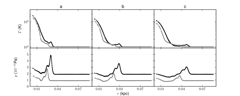
Figure 3: Temperature and pressure profile of the shock wave traveling through a gas with density $\rho=81$ amu cm^-3 and an initial temperature of 10,000 K for timesteps (a) 0.6 Myr, (b) 1.0 Myr, and (c) 1.4 Myr. The black dots represent the old gas physics, the gray ones the new gas physics.

3.1 Simulations

In order to obtain a full understanding of the influence of ionization on the propagation of a shock wave in numerical computations, we conducted a series of SPH-simulations, using a modified version of the cosmological simulation code Gadget2 (Springel, 2005; Valcke et al., 2008). We employ a prescription for artificial thermal conductivity (Price, 2008), that is used to smooth the initial central energy peak during the first few timesteps, and a timestep criterion along the lines of that proposed by Springel (2010), which appropriately increases the number of timesteps used to integrate the motions for a particle just ahead of the shock wave (Saitoh & Makino, 2009). We note that these modifications are crucial to perform high resolution simulations of a Sedov-Taylor blast wave without severe energy losses during the first few timesteps, and without a potentially fatal mistreatment of the initial shock. We ran simulations with two different types of the code: one version which treated the gas as an ideal, fully ionized H plasma with a constant adiabatic index (hereafter denoted as “old” gas physics) and one version where the correct energy and pressure relations are used (dubbed “new” gas physics). In order to implement the new gas physics, we had to replace the entropy equation in Gadget2 with the energy equation, as already noted above.

As initial conditions for our simulations, we used a cubic box with periodic boundary conditions and side 0.1 kpc, wherein a total gas mass of $2\times 10^{6}$ solar masses was sampled using $300,000$ randomly distributed SPH-particles. For 2 Gyr, these particles were first evolved using Gadget2 in order to allow the system to reach an equilibrium density of $\rho=81$ amu cm^-3. This is a value typical for a cold, dense star-forming cloud in a galaxy evolution simulation (see for example Governato et al. (2010); Cloet-Osselaer et al. (2012); Schroyen et al. (2013), who use a density threshold for star formation of up to 100 amu cm^-3). Various initial temperatures, ranging from 100 K to 15,000 K, were used, in order to demonstrate the effect of H ionization. After the system had reached an equilibrium, an energy of $10^{52}$ erg was injected, mimicking the simultaneous energy injection of about 10 supernovae (the typical stellar feedback used in for example Schroyen et al. (2011); Cloet-Osselaer et al. (2012)), by giving this energy to the particle closest to the box center. The system was then evolved using Gadget2.

In order to assess the combined effects of initial temperature and density on our results, we also simulated the expansion of shock waves through gas with densities of 0.81 amu cm^-3 and 0.0081 amu cm^-3, and for the same initial temperatures as listed above. These simulations were set up by sampling a total gas mass which was respectively a factor 100 and a factor 10,000 smaller, using the same procedure as above, within an equally large box. This should give us an idea of how the new gas physics scales with density and together with the different temperatures explored should cover a broad range of scenarios occurring in galaxy evolution simulations.

4 Results

To characterize the resulting shock wave we analysed its radial distance from the box center, which is well quantified by the radius of the SPH particle with the highest density, as a function of time. The results are shown in Fig. 2, for both the old (gray dots, blue in the online version) and the new gas physics (black dots, green in the online version), and are compared with the analytical solution with a constant adiabatic index $\gamma=\frac{5}{3}$ (full black line). The latter is seen to agree very well with the old gas physics, except for the small deviation at the end of the simulation that is caused by boundary effects as the shock wave hits the periodic boundary of the box. There is a clear difference between simulations using the old and the new gas physics; in the latter, the shock wave travels substantially slower. This is due to the fact that part of the shock wave energy is converted into (potential) ionization energy.

The effect is also partially due to the change in mean particle mass, as this will cause the pressure to be lower at temperatures below 10,000 K. To illustrate the contributions of both the change in mean particle mass and the potential energy reservoir, we also plotted the results for simulations only implementing the former in Fig. 2 (gray crosses, red dots in the online version).

To further illustrate the damping of the shock wave, we plotted temperature and pressure profiles for both versions of the gas physics in Fig. 3, for a simulation with initial temperature $T=10,000$ K. The shock wave is visible as the outward propagating temperature and density peak. For the old gas physics (black curves) this peak clearly stands out while for the new gas physics (gray curves) it is strongly suppressed. In the latter case, a substantially smaller fraction of the shock wave’s energy goes into heating the gas and is instead spent ionizing the gas. As a result, the pressure along the shock front is lower for the new gas physics, which results in a slower shock wave propagation. Note also that the overall pressure is lower for the new gas physics, as a result of the higher mean particle mass $\mu(T)$ at the initial temperature.

We plot the ratio of the increase in potential energy to the initial shock wave energy in Fig. 4. For the high density simulations, at least 50 % of the initially injected energy is converted into potential energy for all temperatures. As the gas expands, cools, and recombines after the passage of the shock wave, the potential energy can decline again. For lower densities, this effect is largely compensated by the large increase in shockwave temperature resulting from the much lower density. At 0.81 amu cm^-3, up to 20 % of the shockwave energy is converted into potential energy by the time the shock reaches the box edge. The effect is strongest for low temperatures, as in this case a larger part of the potential energy reservoir is still available for excitation. At the lowest density of 0.0081 amu cm^-3, the total shockwave energy is orders of magnitude higher than the combined contribution of all potential energy terms, so the ratio stays close to zero for the part of the evolution we consider. At these lower densities, the potential energy is roughly proportional to the amount of gas that has been ionized and can hence be expected to be proportional to the volume within the spherically expanding shock wave. Since $r_{s}\propto t^{2/5}$ it follows that we expect $\Delta u_{pot}/u_{shock}\propto t^{6/5}$. This quasi-linear behaviour is indeed observed in the middle and bottom panels of Fig. 4.

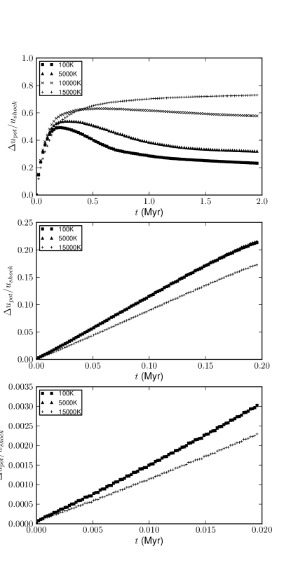
Figure 4: The ratio of the total potential energy change and the injected energy as a function of time for different temperature values close to the ionization temperature of H. Top: gas density of 81 amu cm^-3, middle: gas density of 0.81 amu cm^-3, bottom: gas density of 0.0081 amu cm^-3.

5 Discussion and conclusions

The damping of shock waves has important repercussions in our specific case of galaxy evolution simulations, where supernova feedback is often injected into the interstellar medium as thermal energy. The Sedov-Taylor experiments described here give a fair idea of the effects that can be expected in full-fledged galaxy simulations. Including the new gas physics described here, the expanding bubbles of hot, dilute gas that surround stellar nurseries will propagate more slowly into the surrounding interstellar medium. Moreover, the interstellar gas will be heated less by the supernovae, as part of the feedback energy will be spent on ionizing the gas. A detailed account of the precise effect of our improved description of gas dynamics on simulations of galaxy evolution is the subject of future work (B. Vandenbroucke et al. 2013, in preparation).

To conclude, we have shown how the effects of ionization on the ‘macroscopic’ dynamics of a low-density gas can be taken into account numerically using the proper ‘microscopic’ physics. We have used hydrodynamical simulations to illustrate that employing the improved equation of state and thermal energy density has a significant effect on the propagation of spherically expanding shock waves in a Hydrogen gas. The ionization opens up new degrees of freedom that make the gas behave essentially isothermally when Hydrogen ionizes or recombines. This significantly damps shock waves. We have shown that this limits the efficiency with which supernova-blown shock waves inject energy into the interstellar medium to less than 50 %. We therefore strongly encourage the use of the potential energy term in the expression for the thermal energy density, not only in the case of ionization, but also for other astro-chemical reactions.

We have made tables available online containing the mean particle mass and the specific energy per unit mass as a function of temperature. These are the same tables which were used to perform the simulations in this paper. More details about these tables and the cooling tables associated with them can be found in De Rijcke et al. (2013).

References

- Anninos et al. (1997) Anninos P., Zhang Y., Abel T., Norman M. L. 1997, New Astronomy, 2, 209
- Choi & Wiita (2010) Choi E., Wiita P. J. 2010, ApJS, 191, 113
- Cloet-Osselaer et al. (2012) Cloet-Osselaer A., De Rijcke S., Schroyen J., Dury V. 2012, MNRAS, 423, 735
- De Rijcke et al. (2013) De Rijcke S., Schroyen J., Vandenbroucke B., Jachowicz N., Decroos J., Cloet-Osselaer A., Koleva M., 2013, MNRAS, submitted
- Governato et al. (2010) Governato F., Brook C., Mayer L., Brooks A., Rhee G., Wadsley J., Jonsson P., Willman B., Stinson G., Quinn T., Madau P. 2010, Nature, 463, 203
- Grevesse et al. (2010) Grevesse N., Asplund M., Sauval A. J., Scott P. 2010, Ap&SS, 328, 179
- Landi et al. (2012) Landi E., Del Zanna G., Young P. R., Dere K. P., Mason H. E. 2012, ApJ, 744, 99
- Marek et al. (2009) Marek A., Janka H.-T., Müller E. 2009, A&A, 496, 475
- Mihalas & Mihalas (1984) Mihalas D., Mihalas B. W. 1984, Foundations of radiation hydrodynamics (1st ed.; New York, NY: Oxford University Press)
- Mizuta et al. (2005) Mizuta A., Takabe H., Kane J. O., Remington B. A., Ryutov D. D., Pound M. W. 2005, Ap&SS, 298, 197
- Pakmor et al. (2012) Pakmor R., Edelmann P., Röpke F. K., Hillebrandt W. 2012, MNRAS, 424, 2222
- Price (2008) Price D. J. 2008, J. Comput. Phys., 227, 10040
- Saitoh & Makino (2009) Saitoh T. R., Makino J. 2009, ApJ, 697, L99
- Schroyen et al. (2011) Schroyen J., de Rijcke S., Valcke S., Cloet-Osselaer A., Dejonghe H. 2011, MNRAS, 416, 601
- Schroyen et al. (2013) Schroyen J., de Rijcke S., Koleva M., Cloet-Osselaer A., Vandenbroucke B. 2013, MNRAS, submitted
- Sedov (1977) Sedov L. 1977, Similitude et dimensions en mecanique (7th ed.; Moscou: Editions Mir)
- Shen et al. (2010) Shen S., Wadsley J., Stinson G. 2010, MNRAS, 407, 1581
- Springel (2005) Springel V. 2005, MNRAS, 364, 1105
- Springel (2010) Springel V. 2010, MNRAS, 401, 791
- Springel & Hernquist (2002) Springel V., Hernquist L. 2002, MNRAS, 333, 649
- Stamatellos et al. (2007) Stamatellos D., Whitworth A. P., Bisbas T., Goodwin S. 2007, A&A, 475, 37
- Teyssier (2002) Teyssier R. 2002, A&A, 385, 337
- Valcke et al. (2008) Valcke S., de Rijcke S., Dejonghe H. 2008, MNRAS, 389, 1111
- Verner et al. (1996) Verner D. A., Ferland G. J., Korista K. T., Yakovlev D. G. 1996, ApJ, 465, 487