Bayesian Functional Generalized Additive Models with Sparsely Observed Covariates

Abstract

We propose semiparametric Bayesian methods for scalar-on-function regression involving sparse longitudinal data. Our work extends the functional generalized additive model (FGAM) of [24], a recently proposed model offering greater flexibility than the common functional linear model (FLM). The algorithms we develop allow for the functional covariates to be sparsely observed and measured with error, whereas the estimation procedure of [24] required that they be noiselessly observed on a regular grid. The Bayesian approaches we present estimate the functional predictors simultaneously with all other model parameters, and hence automatically account for variability in the estimated predictors, which is not possible with current frequentist approaches in the literature. We consider both Monte Carlo and variational Bayes methods for fitting the FGAM with sparsely observed covariates. Due to the complicated form of the model posterior distribution and full conditional distributions, standard Monte Carlo and variational Bayes algorithms cannot be used. The strategies we use to handle the updating of parameters without closed-form full conditionals should be of independent interest to applied Bayesian statisticians working with nonconjugate models. Our numerical studies demonstrate the benefits of our algorithms over a two-step approach of first recovering the complete trajectories using standard techniques and then fitting a functional regression model. Our methods are applied to forecasting closing price for items up for auction on the online auction website eBay.

Keywords: auction data, functional data analysis, functional regression, linear mixed models, measurement error, MCMC, penalized splines, variational inference

1 Introduction

In this work, we extend a general class of models for functional regression to the longitudinal data setting, where each sampled function may have only a small number of noisy measurements at irregular time intervals. This setting presents considerable challenges which cannot be handled by conventional estimation methods in the functional regression literature. Previous work in this area assumes a linear relationship between the response and covariate, which is often inappropriate. We build on the work of [24], in order to allow for more general response-predictor relationships. The estimation methods used in [24] depend upon the functional data being fully observed without error. A naive approach of simply interpolating between points for each functional covariate, and then assuming the trajectories are completely observed can be very inaccurate, and we therefore must develop an entirely different approach to [24]. We will take a Bayesian approach, which will allow us to simultaneously recover the complete functional trajectories while estimating all other model parameters.

It is now commonplace in many fields to collect data where each observation is a sample path from some underlying continuous-time stochastic process, $\{X(t):t\in{\mathcal{T}}\}$. Functional data analysis (FDA) is the branch of statistics concerned with methods for analyzing such data. FDA methods often rely on an assumption of smoothness of the underlying process and ordinarily assume the sampled trajectories $X_{i}(t)$ are fully and noiselessly observed. Typically, the $X(t)$ are represented as the result of some presmoothing of the data.

One problem that is frequently studied in the FDA literature is that of using the sampled trajectories as covariates in a regression model involving a scalar response variable. The most commonly used model in this setting is the functional linear model (FLM), first proposed in [31], given by

$$E(Y_{i}\mid X_{i})=\theta_{0}+\int_{\mathcal{T}}\beta(t)X_{i}(t)\,dt,\quad i=1,\ldots,N;$$ (1)

where $X_{i}$ is a real-valued, continuous, square-integrable, random curve on the compact interval ${\mathcal{T}}$, $Y_{i}$ is a scalar random variable, $\theta_{0}$ an intercept, and $\beta(\cdot)$ is the functional coefficient with $\beta(t)$ describing the effect on the response of the functional predictor at time $t$.

A model recently proposed in [24] called the functional generalized additive model (FGAM) removes the restrictive linearity assumption of the FLM by modeling the conditional mean of $Y$ as

$$E(Y_{i}\mid X_{i})=\eta_{0i}+\int_{\mathcal{T}}F\{X_{i}(t),t\}\,dt,$$ (2)

where $F$ is an unknown smooth function and the offset term $\eta_{0i}$ contains any additional scalar or functional covariates other than $X_{i}(t)$. Notice that as a special case, when $F\{X(t),t\}=\beta(t)X(t)$ and $\eta_{0i}=\theta_{0}$, we obtain the FLM. This model retains the ease of interpretability of the FLM while suffering from less approximation bias. The surface $F$ will be parameterized using tensor products of B-splines and two smoothing parameters will control the complexity of the estimated surface. As the FLM can be thought of as a (multivariate) linear model with an infinite number of predictors, the FGAM can be thought of as an additive model in an infinite number of predictors [24].

Frequently, the functional data we encounter in practice are not observed on a dense, regularly-spaced grid, but instead on a sparse, irregular grid with measurement error and with some subjects having as little as one or two measurements. This type of data is frequently found in the longitudinal data analysis (LDA) literature. An overview of the differences between FDA and LDA can be found in [32]. When the trajectories are not observed on a regular grid, the estimation procedure used in [24] cannot be directly applied. In these situations, the semiparametric techniques commonly used in LDA are more appropriate; in this work, we take a linear mixed effects modeling approach. Most of the previous work on sparsely observed functional data only considers estimation of the mean and covariance function of the underlying process, with few papers examining regression of a scalar on the sparse trajectories. Notable exceptions are [17], [41], [1], and [12]. To the best of our knowledge, our work is the first to study nonparametric regression with sparse functional data.

It is common to estimate the complete functional trajectories by performing a functional principal components analysis (FPCA); for example, the principal components analysis through conditional expectation (PACE) method of [48]. Whereas a typical functional data analysis smooths the measurements for each subject separately, the advantage of PACE is that it pools data across subjects at each time point to estimate an entire covariance surface. This “borrowing of strength” across subjects is a main reason for the method’s success. Although it is not considered in [48], one might think it reasonable to use a two-stage approach of first using PACE to recover the function predictors and then in a second step fitting an FLM using standard techniques or an FGAM using the procedure in [24]. The main advantage of our Bayesian algorithms over a two-stage approach is that they allow us to directly account for uncertainty in the estimates from the FPCA. Our numerical results demonstrate the inadequacy of a conventional two-stage estimation procedure and we believe that our algorithms also gain from using information in the response when estimating the functional trajectories.

An important step in the PACE procedure is estimating the covariance surface of the functions using local polynomial modeling. Although PACE often performs well in a variety of situations, in our simulation studies we observe similar results to [29], who found that PACE can have problems in more challenging settings with higher sparsity and a true covariance function that has more than three non-zero eigenvalues. In a number of the simulations in [29], and in our own experiments, the covariance surface estimated by PACE is not positive definite and the estimated measurement error variance is negative. We will demonstrate that our Bayesian algorithms do not suffer from this problem. Our methods can also be used to effectively recover a greater number of principal components. Several currently available techniques only consider recovery of two non-zero principal components in simulation studies and attempt to estimate three components in real data studies [48, 47, e.g.,].

Our goals are three-fold: 1) accurate recovery of the sparsely observed trajectories, 2) accurate recovery of the surface, $F(x,t)$, and 3) accurate prediction of the response, $Y$. The missing parts of the trajectories must be imputed during the estimation procedure. Three possibilities for doing this are an expectation-maximization (EM) algorithm, Markov Chain Monte Carlo (MCMC), or a variational approximation. The advantage of MCMC over an EM algorithm approach is that uncertainty about the imputed curves is automatically taken into account during the estimation. Due to the computational overhead associated with MCMC, we also present a variational Bayes algorithm that can be used for fast approximate inference and to initialize an MCMC sampler.

Variational Bayes (VB) refers to a specific variational approximation used for Bayesian inference that relies on the assumption that a posterior density of interest factors into a product form over certain groups of model parameters. Though they are commonly used in computer science, the application of variational approximations in statistics is relatively new; [28] provides an overview. When the amount of posterior dependence is small, there is little loss of accuracy and often very large improvements in computation time over MCMC methods. Applications of VB to regression problems with missing data can be found in [9] and [14], the latter of which considered the FLM.

The success of the approximation hinges on the amount of between-group dependence among the parameters in the posterior distribution. The cost of the computational efficiency gains from the approximations made in VB is the loss of guaranteed convergence to the correct distribution provided by MCMC. Factorization assumptions are often reasonable for certain groups of parameters in functional data models [14]. We agree with those authors that VB should not be considered a replacement for fully Bayesian inference. Instead we consider it as complementary to MCMC: a useful tool for approximate answers in large data situations when MCMC becomes intractable. One natural way to use the two as complements is to use VB estimates as starting values for an MCMC algorithm in the hopes of achieving faster convergence to, and better exploration of, the posterior distribution of interest. In our experience, the choice of starting values is critical for high-dimensional problems such as functional regression.

When conjugate priors are used and closed-form expressions exist for all full conditional distributions in a model, the optimal densities for approximating the posterior using VB have closed-form expressions as well. It is not possible to obtain closed-form updates for all the paramaters in the FGAM due to the nonconjugate full conditional distribution for the principal component scores, as they appear in the likelihood as arguments to the B-spline basis functions used to parameterize the regression surface. Therefore, Metropolis-Hasting steps are needed for our MCMC algorithm. For our VB algorithm, we alternatively overcome the nonconjugacy using a Laplace approximation. An additional complication is the necessity of an anisotropic roughness penalty for $F(x,t)$, owing to the possibly differing amounts of smoothness in $x$ and $t$, which makes the two smoothing parameters difficult to separate. Using our VB approach, we are typically able to obtain a speed-up of at least an order of magnitude over generating 10,000 samples from our MCMC sampler, with minimal sacrifice in accuracy. Our approaches perform quite well at both out-of-sample prediction and recovering the true surface whether the true model is linear or nonlinear.

The remainder of the paper proceeds as follows: Section 2 briefly reviews functional principal component analysis, Section 3 discusses our parameterization for the unknown surface, $F(x,t)$, Section 4 discusses our MCMC algorithm for fitting FGAM, Section 5 reviews variational Bayes and provides a VB algorithm for fitting FGAM, Section 6 discusses results of simulation experiments, in Section 7 we apply our algorithms to forecasting closing prices for seven day auctions on the auction website eBay, and Section 8 concludes.

2 Recovering Sparsely Observed Functional Data

In this section we give a brief overview of the literature on estimating trajectories from sparsely observed functional data; one of our goals mentioned in the previous section and a key step in building our regression model. Most methods involve various techniques for estimating eigenfunctions and eigenvalues from an FPCA. A common approach for this is to use mixed model representations for penalized or smoothing splines; see [18] and the references therein. Another frequently used approach uses local polynomial modeling; see e.g., [48]. Bayesian approaches to functional data analysis include the wavelet-based mixed model method of [25] and the Dirichlet process based approach of [33]. Though some papers in the Bayesian literature, including the ones cited above, appear to be able to deal with irregularly sampled functional data, it is unclear how these methods perform in the high-sparsity situations we wish to consider here, and we are not aware of any of these papers analyzing how their methods perform under varying degrees of sparsity/missingness.

The usual model for the unknown functions is to assume $n_{i}$ noisy measurements have been taken of $X_{i}(t)$: ${\widetilde{\mathbf{x}}}_{i}=\{\widetilde{x}_{i}(t_{i,1}),\ldots,\widetilde{x}_{i}(t_{i,n_{i}})\}^{T}$ with $\widetilde{x}_{i}(t_{ij})=X_{i}(t_{ij})+e_{ij};\ e_{ij}\stackrel{{\scriptstyle\text{i.i.d.}}}{{\sim}}N(0,\sigma^{2}_{x});\ i=1,\ldots,N;\ j=1,\ldots,n_{i}.$ We define the mean and covariance functions $\mu_{x}(t):=E\{X(t)\}$ and $G(s,t):=\text{Cov}\{X(s),X(t)\}$. If $X\in\mathcal{L}^{2}$, then by Mercer’s theorem $G(s,t)$ admits an expansion $G(s,t)=\sum^{\infty}_{m=1}\nu_{m}\phi_{m}(s)\phi_{m}(t)$ with (orthonormal) eigenfunctions $\phi_{m}(\cdot)$ and associated eigenvalues $\nu_{m}$, and the curves have a Karhunen-Loève representation $X_{i}(t)=\mu_{x}(t)+\sum^{\infty}_{m=1}\phi_{m}(t)\xi_{im};\ \xi_{im}\stackrel{{\scriptstyle{\mbox{\scriptsize ind.}}}}{{\sim}}(0,\nu_{m})$, where the $\xi$’s are known as principal component (PC) scores. If $X(t)$ is assumed to be a Gaussian process, then the principal component scores are Gaussian random variables.

For all FPCA methods, it is necessary to choose an integer, $M$, at which to truncate the basis expansion for the unknown functions (i.e. assume $\xi_{k}=0$ for all $k>M$). This is typically done by including enough scores to explain a prespecified percentage (e.g. $99\%$) of the total observed variation in the data, and that is the approach we take in our analysis of the auction data in Section 7.

To initialize both our MCMC and VB algorithms, we take a similar (though not identical) approach to [48]. We use P-splines [8] for the smoothing steps 1. and 2. described below whereas [48] took a local polynomial modelling approach for these steps. The use of penalized splines to perform FPCA is covered in detail by [47]. We perform the smoothing using the R package mgcv [43] and use generalized cross validation to choose smoothing parameters. The full list of steps for performing the FPCA are as follows.

1. Obtain an estimate $\widehat{\mu}(t)$ of $\mu(t)$ via semiparametric regression of the pooled data ${\widetilde{\mathbf{x}}}=({\widetilde{\mathbf{x}}}_{1}^{T},\dots,{\widetilde{\mathbf{x}}}_{N}^{T})^{T}$ on $\widetilde{{\mathbf{t}}}=({\mathbf{t}}_{1}^{T},\ldots,{\mathbf{t}}_{N}^{T})^{T}$; ${\mathbf{t}}_{i}=(t_{i,1},\ldots,t_{i,n_{i}})^{T}$ using P-splines.

2. Obtain an estimate $\widehat{G}(s,t)$ of $G(s,t)$ by fitting a cubic tensor-product P-spline [23] to the “raw” covariances with the diagonal removed: $\{\widetilde{x}_{i}(t_{il})-\widehat{\mu}_{x}(t_{il})\}\{\widetilde{x}_{i}(t_{is})-\widehat{\mu}_{x}(t_{is})\},\ l\neq s$. We use third-derivative penalties when fitting the tensor product spline in order to shrink estiamte towards a quadratic surface. We write $\widehat{G}({\mathbf{t}}_{i},{\mathbf{t}}_{i})$ to denote the $N_{i}\times N_{i}$ matrix with $(j,k)$-entry $\widehat{G}(t_{ij},t_{ik})$.

3. $\sigma_{x}^{2}$ is estimated as the average of the middle two thirds of the diagonal of the raw covariance matrix minus the diagonal of the smoothed covariance surface. This is as in [48] and is done to avoid boundary effects.

4. ${\widehat{\bm{\nu}}}=(\widehat{\nu}_{1},\ldots,\widehat{\nu}_{M})^{T},\text{ and }\widehat{\phi}_{1}(t),\ldots,\widehat{\phi}_{M}(t)$ are obtained as the eigenvalues and eigenvectors, respectively, from an eigendecomposition of the estimated covariance matrix.

5. The principal component scores are the best linear unbiased prediction (BLUP) estimates:

   $${\widehat{\bm{\xi}}}_{i}=\operatorname{{{diag}}}(\widehat{{\bm{\nu}}})\widehat{\bm{\Phi}}({\mathbf{t}}_{i})^{T}\{\widehat{G}({\mathbf{t}}_{i},{\mathbf{t}}_{i})+\widehat{\sigma}_{x}^{2}{\mathbb{I}}_{N_{i}}\}^{-1}\{\widetilde{{\mathbf{x}}}_{i}-\widehat{{\bm{\mu}}}_{x}({\mathbf{t}}_{i})\},$$

   ${\widehat{\bm{\xi}}}_{i}=(\widehat{\xi}_{i1},\ldots,\widehat{\xi}_{iM})^{T}$, and $\widehat{\bm{\Phi}}({\mathbf{t}}_{i})=[\widehat{\bm{\phi}}_{1}({\mathbf{t}}_{i}):\cdots:\widehat{\bm{\phi}}_{M}({\mathbf{t}}_{i})]$, where $\widehat{{\bm{\phi}}}_{j}({\mathbf{t}}_{i})$ and ${\widehat{\bm{\mu}}}_{x}({\mathbf{t}}_{i})$ denotes the vector of evaluations of the $j$th estimated eigenfunction and estimated mean function, respectively, at the timepoints ${\mathbf{t}}_{i},\ i=1,\ldots,N.$

The parameters $M$, $\mu(t),\ \nu_{1},\ldots,\nu_{M},\text{ and }\phi_{1}(t),\ldots,\phi_{M}(t)$ are fixed at these initial estimates for our MCMC and VB algorithms. This is as done in [14], though they do update $\nu_{1},\dots,\nu_{M}$. For ease of notation, we suppress the “hat”/circumflex for these parameters when developing our algorithms in later sections. The principal component scores as well as the measurement error variance are updated by both algorithms, and we will demonstrate that our methods can be used to accurately estimate more principal components beyond the first two. This procedure is also used in our numerical experiments when, for comparison, we also estimate FGAM using the two-step approach mentioned in the introduction.

3 Penalized Spline Smoothing For FGAM

3.1 Review of Tensor Product Splines

We next discuss our representation for the bivariate surface $F(\cdot,\cdot)$ in (2). We choose to use penalized splines which are very popular tools for applied regression modelling. Book-length treatments of penalized splines are provided by [34, 43]. We use tensor product splines to approximate $F(x,t)$. In this approach, the bivariate function $F$ is constructed from univariate splines in $x$ and $t$ as follows. First, considering a univariate function, $f$ of $x$, we may represent $f(x)$ using splines as $f(x)=\sum_{j=1}^{K_{x}}\gamma_{j}B^{X}_{j}(x)$, where the $\gamma_{j}$ are spline coefficients to be estimated from the data and $\{B^{X}_{1}(x),\ldots,B^{X}_{K_{x}}(x)\}$ is a prespecified $K_{x}$-dimensional spline basis over the possible values of $x$. We add dependence on $t$ by considering the spline coefficients to be functions of $t$, which we again approximate using splines; i.e. $\gamma_{j}(t)=\sum_{k=1}^{K_{t}}\theta_{jk}B_{k}^{T}(t)$; $j=1,\ldots,K_{t}$; where $\{B^{T}_{1}(t),\ldots,B^{T}_{K_{t}}(t)\}$ is a spline basis for the $t$-axis. Combining the equations for $f(x)$ and the $\gamma_{j}(t)$’s we have the following tensor product spline representation for $F(x,t)$ [44, e.g.,]

$$F(x,t)=\sum_{j=1}^{K_{x}}\sum_{k=1}^{K_{t}}\theta_{jk}B_{j}^{X}(x)B_{k}^{T}(t).$$ (3)

We use B-splines for the basis functions, which are popular because of their good numerical properties and for their computational convenience. An introduction to univariate and tensor product B-splines is provided in [7, Ch. 1,2]. To fit a tensor product spline model, one must specify a polynomial degree for the univariate spline bases; the number of knots for the spline bases, $K_{x}$ and $K_{t}$, as well as their location; penalty parameters, $d_{x}$ and $d_{t}$; and smoothing parameters, $\lambda_{x}$ and $\lambda_{t}$ which control the trade-off between fitting the data (minimizing mean square error) and complexity of $F(\cdot,\cdot)$. While this may seem like a lot of parameters to specify, in practice assuming that $K_{x}$ and $K_{t}$ are chosen to be large enough, the most important factor determining the fit of the spline is the choice of smoothing parameters [35], and the knots are almost always specified to be equally-spaced distances apart. The degree of the spline bases is typically chosen to be three, i.e. cubic splines and the penalty parameters, which we discuss in more detail shortly, are both chosen to be two, so that the surface is shrunk towards a plane with increasing $\lambda_{x}$ and $\lambda_{t}$ [8]. The cubic B-spline pairs, $B^{X}_{j}(x)B^{T}_{k}(t)$, look like overlapping “humps” or standard bivariate normal densities.

Plugging (3) into (2) we obtain

$$E(Y_{i}\mid X_{i}) =\eta_{0i}+\int F\{x_{i}(t),t\}\,dt\approx\eta_{0i}+\sum^{K_{x}}_{j=1}\sum^{K_{t}}_{k=1}\int B^{\mathcal{X}}_{j}\{x_{i}(t)\}B^{\mathcal{T}}_{k}(t)\theta_{j,k}\,dt$$

The integral above must be approximated via quadrature. We specify a grid of time points ${\mathbf{t}}=(t_{1},\ldots,t_{T})^{T}$ where the integral is to be evaluated and define a vector of quadrature weights, ${\mathbf{L}}=(L_{1},\ldots,L_{T})^{T}$. The estimated trajectories and the B-spline bases are evaluated at ${\mathbf{t}}$, which results in the vectors ${\mathbf{x}}_{i}=\{x_{i}(t_{1}),\dots,x_{i}(t_{T})\}^{T}$; i=1,…,N; ${\mathbf{B}}^{\mathcal{X}}_{j,i}=[B^{\mathcal{X}}_{j}\{x_{i}(t_{1})\}$, $\dots,B^{\mathcal{X}}_{j}\{x_{i}(t_{T})\}]^{T}$; and ${\mathbf{B}}^{\mathcal{T}}_{k}=\{B^{\mathcal{T}}_{k}(t_{1}),\dots,B^{\mathcal{T}}_{k}(t_{T})\}^{T}$. For the $i$th subject and $(j,k)$ basis function pair, we have $\int B^{X}_{j}\{x_{i}(t)\}B^{T}_{k}(t)\,dt\approx{\mathbf{L}}^{T}({\mathbf{B}}^{\mathcal{X}}\odot{\mathbf{B}}^{\mathcal{X}})$, where $\odot$ denotes element-wise multiplication. We then arrive at the following approximation to (2) which we use for the rest of the paper

$$E(Y_{i}\mid X_{i})=\eta_{0i}+\int F\{x_{i}(t),t\}\,dt\approx\eta_{0i}+\sum^{K_{x}}_{j=1}\sum^{K_{t}}_{k=1}{\mathbf{L}}^{T}({\mathbf{B}}^{\mathcal{X}}_{j,i}\odot{\mathbf{B}}^{{\mathcal{T}}}_{k})\theta_{j,k}=\eta_{0i}+\sum^{K_{x}}_{j=1}\sum^{K_{t}}_{k=1}Z_{j,k,i}\theta_{j,k}.$$ (4)

Recalling our estimate for the trajectories from the previous section, for ease of notation, we will write ${\bm{\mu}}_{x}({\mathbf{t}})$ and ${\bm{\Phi}}({\mathbf{t}})$ as ${\bm{\mu}}_{x}$ and ${\bm{\Phi}}$, respectively, and only specify the grid of evaluation points if it differs from ${\mathbf{t}}$. In the calculations that follow, we frequently work with the $T\times K_{x}K_{t}$ matrix of B-spline products evaluated at the grid points, ${\mathbf{t}}$, and estimated trajectories, ${\mathbf{x}}_{i}={\bm{\mu}}_{x}+{\bm{\Phi}}{\bm{\xi}}_{i}$:

$${\mathbb{B}}_{\xi_{i}}=\mathopen{}\mathclose{{}\left[\{B_{1}^{X}({\bm{\mu}}_{x}+{\bm{\Phi}}{\bm{\xi}}_{i})\cdots B_{K_{x}}^{X}({\bm{\mu}}_{x}+{\bm{\Phi}}{\bm{\xi}}_{i})\}\otimes\mathbf{1}^{T}_{K_{t}}}\right]\odot\mathopen{}\mathclose{{}\left[\mathbf{1}_{K_{x}}^{T}\otimes\{B_{1}^{T}({\mathbf{t}})\cdots B_{K_{t}}^{T}({\mathbf{t}})\}}\right],\quad i=1,\ldots,N,$$ (5)

where $\otimes$ denotes the Kronecker product. This matrix is always multiplied on the left by the vector of quadrature weights, ${\mathbf{L}}$, so we also define ${{\mathbf{b}}_{{\bm{\xi}}_{i}}^{T}}\equiv{\mathbf{L}}^{T}{{\mathbb{B}}_{{\bm{\xi}}_{i}}}$. Note that ${{\mathbf{b}}_{{\bm{\xi}}_{i}}^{T}}=(Z_{1,1,i},\dots,Z_{K_{x},K_{t},i})^{T}$ is the $i$th row of the matrix ${\mathbb{Z}}$ from [24].

3.2 Formulation as a Mixed Model

The mixed model formulation of penalized splines is now well-known and widely-used, see e.g., for a review. The FGAM looks superficially like a bivariate smoothing problem, but it is more challenging since we do not observe $F(x,t)$ (with error) for pairs $(x,t)$ but instead we observe only the integral of $F\{X(t),t\}$ with respect to $t$. Nonetheless, some ideas from bivariate smoothing are applicable to FGAM. As in [24], we start with a bivariate spline model for $F(\cdot,\cdot)$ based on P-splines [8, 23]. We take a more general approach than the Bayesian P-splines of [21], which performed isotropic smoothing via a first-order Gaussian random walk prior for the bivariate components in their additive model.

Frequently in the penalized spline literature it is assumed $\lambda_{x}=\lambda_{t}$ to simplify estimation. Here however, because $X(t)$ and $t$ having differing scales, it is not appropriate to assume apriori that the amount of smoothing for $F(x,t)$ should be the same in both arguments. Though we may scale $x$ and $t$ to lie in the unit square, this would still not result in a scale-invariant tensor product smooth [46]. The necessitated anisotropic roughness penalty associated with the spline coefficients, ${\bm{\theta}}=(\theta_{11},\dots,\theta_{1,K_{t}},\theta_{2,1}\dots,\theta_{K_{x},K_{t}})^{T}$, requires considerable more care than the univariate smoothing necessary for the Bayesian FLM in [12], the isotropic penalty used in [26], or the penalized structured additive regression literature [10, e.g.,].

[38] first made the connection between spline smoothing and Bayesian modeling, showing that the usual (frequentist) estimator for a cubic smoothing spline was equivalent to placing a particular improper Gaussian prior on the spline coefficients. The penalization used in [24] is equivalent to imposing the following prior on the spline coefficients

$$p({\bm{\theta}}\mid\lambda_{x},\lambda_{t})\propto\exp\mathopen{}\mathclose{{}\left(-\frac{1}{2}{\bm{\theta}}^{T}{\mathbb{P}}_{\bm{\theta}}(\lambda_{x},\lambda_{t}){\bm{\theta}}}\right),$$

with ${\mathbb{P}}_{\bm{\theta}}(\lambda_{x},\lambda_{t})=\lambda_{x}{\mathbb{P}}_{x}+\lambda_{t}{\mathbb{P}}_{t}$, with ${\mathbb{P}}_{x}={\mathbb{D}}_{x}^{T}{\mathbb{D}}_{x}\otimes{\mathbb{I}}_{K_{t}}$, ${\mathbb{P}}_{t}={\mathbb{I}}_{K_{x}}\otimes{\mathbb{D}}_{t}^{T}{\mathbb{D}}_{t}$. ${\mathbb{I}}_{p}$ is the identity matrix of dimension $p$, ${\mathbb{D}}_{t}$ and ${\mathbb{D}}_{x}$ are difference operator matrices of the prespecified degrees, $d_{x}$ and $d_{t}$, respectively. This penalty structure leads to a partially improper Gaussian prior since ${\mathbb{P}}_{\bm{\theta}}(\lambda_{x},\lambda_{t})$ is rank deficient: ${\mathbb{D}}_{x}^{T}{\mathbb{D}}_{x}$ has rank $K_{x}-d_{x}$, ${\mathbb{D}}_{t}^{T}{\mathbb{D}}_{t}$ has rank $K_{t}-d_{t}$, so that ${\mathbb{P}}_{\bm{\theta}}(\lambda_{x},\lambda_{t})$ has rank $K_{x}K_{t}-d_{x}d_{t}$ [15, Section 4.4]. To avoid numerical instability associated with inversion of numerically rank-deficient matrices when sampling from the full conditional of ${\bm{\theta}}$ and the appearance of the zero determinant of ${\mathbb{P}}_{\bm{\theta}}(\lambda_{x},\lambda_{t})$ in the full conditionals of $\lambda_{x}$ and $\lambda_{t}$, we aim for a simpler representation of the function by employing the mixed model representation of tensor product splines used in [5, Section 6]. The idea is to simultaneously diagonalize the marginal penalties for $x$ and $t$. This results in a diagonal penalty structure which is efficient for computations and easy to interpret.

More precisely, we split the function $F(x,t)$ into an unpenalized part parameterizing functions from the nullspace of the penalty (i.e., associated with a diffuse Gaussian prior on the coefficients) and a penalized part (associated with a non-diffuse Gaussian prior on the coefficients). We begin by rewriting the vector of function evaluations for subject $i$ as $F({\mathbf{x}}_{i},{\mathbf{t}})=\sum^{K_{x}}_{j}\sum^{K_{t}}_{k}({\mathbf{B}}^{\mathcal{X}}_{j,i}\odot{\mathbf{B}}^{\mathcal{T}}_{k})\theta_{j,k}={\mathbb{B}}_{\xi_{i}}{\bm{\theta}}.$ We take the spectral decompositions of the marginal penalties, i.e.,

$${\mathbb{D}}_{x}^{T}{\mathbb{D}}_{x}={\mathbb{V}}_{x}{\mathbb{S}}_{x}{\mathbb{V}}_{x}^{T},\;{\mathbb{D}}_{t}^{T}{\mathbb{D}}_{t}={\mathbb{V}}_{t}{\mathbb{S}}_{t}{\mathbb{V}}_{t}^{T},$$

where both ${\mathbb{V}}_{x}$ and ${\mathbb{V}}_{t}$ are orthogonal matrices and ${\mathbb{S}}_{x}$ and ${\mathbb{S}}_{t}$ are diagonal. We define $\widetilde{{\mathbb{V}}}_{x}\text{ and }\widetilde{{\mathbb{V}}}_{t}$ to be the matrices of eigenvectors associated with zero eigenvalues, which have dimension $K_{x}\times d_{x}\text{ and }K_{t}\times d_{t},$ respectively. The basis functions for the unpenalized part of the tensor product spline can then be defined as ${\mathbb{B}}_{i,0}={\mathbb{B}}_{\xi_{i}}(\widetilde{{\mathbb{V}}}_{t}\otimes\widetilde{{\mathbb{V}}}_{x})$,

For the basis for the penalized part of the tensor product spline, ${\mathbb{B}}_{i,p}$, we first define ${\mathbb{S}}_{t,x}=({\mathbb{I}}_{K_{t}}\otimes{\mathbb{S}}_{x})+({\mathbb{S}}_{t}\otimes{\mathbb{I}}_{K_{x}})$, a matrix that has all combinations of sums of the eigenvalues on the diagonal, and form $\widetilde{{\mathbb{S}}}_{t,x}$, which is ${\mathbb{S}}_{t,x}$ without the zero entries on the diagonal corresponding to ${\mathbb{B}}_{i,0}$. This can be written as $\widetilde{{\mathbb{S}}}_{t,x}={\mathbb{U}}^{T}{\mathbb{S}}_{t,x}{\mathbb{U}}$, where ${\mathbb{U}}$ is a $K_{x}K_{t}\times(K_{x}K_{t}-d_{x}d_{t})$ orthogonal matrix constructed by removing $d_{x}d_{t}$ columns from ${\mathbb{I}}_{K_{x}K_{t}}$. We thus have

$${\mathbb{B}}_{i,p}={\mathbb{B}}_{\xi_{i}}({\mathbb{V}}_{t}\otimes{\mathbb{V}}_{x}){\mathbb{U}}\widetilde{{\mathbb{S}}}_{t,x}^{-1/2},\text{ so that }{\mathbb{B}}_{\xi_{i}}{\bm{\theta}}={\mathbb{B}}_{i,0}{\bm{\beta}}+{\mathbb{B}}_{i,p}{\bm{\delta}}$$

or, for clearer exposition,

$${\mathbb{B}}_{\xi_{i}}{\bm{\theta}}=({\mathbb{B}}_{\xi_{i}}{\mathbb{T}})({\mathbb{T}}^{-1}{\bm{\theta}})\text{ with }{\mathbb{T}}=[{\mathbb{T}}_{0}:{\mathbb{T}}_{p}]=\mathopen{}\mathclose{{}\left[\begin{array}[]{*{2}{c}}(\widetilde{{\mathbb{V}}}_{t}\otimes\widetilde{{\mathbb{V}}}_{x}):({\mathbb{V}}_{t}\otimes{\mathbb{V}}_{x}){\mathbb{U}}\widetilde{{\mathbb{S}}}_{t,x}^{-1/2}\end{array}}\right],$$

and ${\mathbb{T}}^{-1}=\mathopen{}\mathclose{{}\left[\begin{array}[]{*{2}{c}}(\widetilde{{\mathbb{V}}}_{t}\otimes\widetilde{{\mathbb{V}}}_{x}):({\mathbb{V}}_{t}\otimes{\mathbb{V}}_{x}){\mathbb{U}}\widetilde{{\mathbb{S}}}_{t,x}^{1/2}\end{array}}\right]^{T}$.

The penalty matrix ${\mathbb{P}}_{\bm{\theta}}(\lambda_{x},\lambda_{t})$ of the reparameterized coefficient vector $({\bm{\beta}}^{T},{\bm{\delta}}^{T})^{T}={\mathbb{T}}^{-1}{\bm{\theta}}$ becomes $\widetilde{{\mathbb{P}}}_{\bm{\theta}}(\lambda_{x},\lambda_{t})=$ ${\mathbb{T}}^{T}{\mathbb{P}}_{\bm{\theta}}(\lambda_{x},\lambda_{t}){\mathbb{T}}.$ Since ${\mathbb{P}}_{\bm{\theta}}(\lambda_{x},\lambda_{t}){\mathbb{T}}_{0}=0$, only the lower right $(K_{x}K_{t}-d_{x}d_{t})\times(K_{x}K_{t}-d_{x}d_{t})$-quadrant of $\widetilde{{\mathbb{P}}}_{\bm{\theta}}(\lambda_{x},\lambda_{t})$ is of interest. Denoting this submatrix by $\widetilde{{\mathbb{P}}}_{\bm{\delta}}(\lambda_{x},\lambda_{t})$, our penalty is now given by the diagonal matrix

$$\widetilde{{\mathbb{P}}}_{\bm{\delta}}(\lambda_{x},\lambda_{t})=\lambda_{t}{\bm{\Psi}}_{t}+\lambda_{x}{\bm{\Psi}}_{x};\quad{\bm{\Psi}}_{t}=\widetilde{{\mathbb{S}}}_{t,x}^{-1/2}{\mathbb{U}}^{T}({\mathbb{S}}_{t}\otimes{\mathbb{I}}_{K_{x}}){\mathbb{U}}\widetilde{{\mathbb{S}}}_{t,x}^{-1/2};\quad{\bm{\Psi}}_{x}={\mathbb{I}}_{K_{x}K_{t}-d_{x}d_{t}}-{\bm{\Psi}}_{t};$$

see [5].

Recalling that ${{\mathbf{b}}_{{\bm{\xi}}_{i}}^{T}}={\mathbf{L}}^{T}{\mathbb{B}}_{\xi_{i}}$ with ${\mathbb{B}}_{\xi_{i}}$ given by (5), we can now write

$$\int F(X_{i}(t),t)\,dt\approx{{\mathbf{b}}_{{\bm{\xi}}_{i}}^{T}}{\bm{\theta}}={\mathbf{L}}^{T}{\mathbb{B}}_{\xi_{i}}{\mathbb{T}}\binom{{\bm{\beta}}}{{\bm{\delta}}}={\mathbf{L}}^{T}{\mathbb{B}}_{\xi_{i}}{\mathbb{T}}_{0}{\bm{\beta}}+{\mathbf{L}}^{T}{\mathbb{B}}_{\xi_{i}}{\mathbb{T}}_{p}{\bm{\delta}}={\mathbf{L}}^{T}{\mathbb{B}}_{i,0}{\bm{\beta}}+{\mathbf{L}}^{T}{\mathbb{B}}_{i,p}{\bm{\delta}}.$$

We use diffuse inverse gamma (IG) priors for the variance components and our full model is given by

$$Y_{i} \sim N(\eta_{0i}+{\mathbf{L}}^{T}{\mathbb{B}}_{i,0}{\bm{\beta}}+{\mathbf{L}}^{T}{\mathbb{B}}_{i,p}{\bm{\delta}},\sigma^{2});\quad\sigma^{2}\sim\text{IG}(a_{e},b_{e});$$

$$\widetilde{{\mathbf{x}}}_{i}({\mathbf{t}}_{i}) \sim N(\mu_{x}({\mathbf{t}}_{i})+{\bm{\Phi}}({\mathbf{t}}_{i}){\bm{\xi}}_{i},\sigma^{2}_{x}{\mathbb{I}}_{n_{i}});\quad\sigma_{x}^{2}\sim\text{IG}(a_{x},b_{x});$$

$$\xi_{im} \sim N(0,\nu_{m});\quad m=1,\ldots,M;$$ (6)

$${\bm{\delta}} \sim N\mathopen{}\mathclose{{}\left(0,[\lambda_{t}{\bm{\Psi}}_{t}+\lambda_{x}{\bm{\Psi}}_{x}]^{-1}}\right);\quad\lambda_{x},\lambda_{t}\sim\text{Gamma}(a_{l},b_{l});$$

$${\bm{\beta}} \sim N(0,\sigma_{\beta}^{2}{\mathbb{I}}_{d_{x}d_{t}});\quad\eta_{0i}\sim N(0,\sigma_{\eta}^{2});\quad i=1,\ldots,N$$

4 An MCMC algorithm for fitting FGAM

We now describe an MCMC algorithm for fitting FGAM. We will use a Metropolis-within-Gibbs sampler. The conjugate priors used for the spline coefficients and the variance components (excluding the smoothing parameters) in our hierarchical model allow for closed-form expressions for those parameters’ full conditional distributions. Since their derivations are quite standard, we omit the details until Appendix A and focus in this section on the more complicated updates for the smoothing parameters and principal component scores.

To understand what is being updated and in what order, we start by providing pseudocode outlining the updates made by our MCMC algorithm to sample the posterior of model (6). Details of how the updates are done will be provided subsequently.This pseudocode also applies to our variational Bayes algorithm developed in the next section; the change being that instead of parameters being updated by randomly drawing from a distribution that converges in the limit to the true posterior distribution (subject to regularity conditions), they are deterministic updates of hyperparameters and moments of optimal densities. The pseudocode is given in Algorithm 1.

Algorithm 1 Pseudocode for fitting FGAM given by (6)

1:Obtain initial estimates, ${\mathbf{x}}$, for the trajectories using the method from Section 2.

2:Specify penalties and bases for $F(x,t)$. Obtain decomposition from Section 3.

3:Initialize other parameters.

4:repeat

5:     for $i=1\to N$ do

6:         Update principal component scores, ${\bm{\xi}}_{i}$.

7:         Update ${\mathbf{x}}_{i}$.

8:         Update ${\mathbb{B}}_{i,p}$.

9:     end for

10:     for $i=1\to N$ do

11:         Update terms involving scalar covariates, $\eta_{0i}$.

12:     end for

13:     Update unpenalized spline coefficients, ${\bm{\beta}}$.

14:     Update penalized spline coefficients, ${\bm{\delta}}$.

15:     Update smoothing parameters, $\lambda_{x},\ \lambda_{t}$.

16:     Update measurement error variance, $\sigma_{x}^{2}$.

17:     Update response error variance, $\sigma^{2}$.

18:until Maximum number of iterations reached OR [for VB] convergence criteria met.

The updates for $\lambda_{x}$ and $\lambda_{t}$ require special attention because of the non-conjugality of their full conditional distributions. To see this, we have

$$p(\lambda_{x}\mid\text{rest}) =p(\lambda_{x}\mid\lambda_{t},{\bm{\delta}})\propto p({\bm{\delta}}\mid\lambda_{x},\lambda_{t})p(\lambda_{x})\propto\lvert\lambda_{x}{\bm{\Psi}}_{x}+\lambda_{t}{\bm{\Psi}}_{t}\rvert^{1/2}(\lambda_{x})^{a_{l}+1}\exp\{-(b_{l}+\frac{1}{2}{\bm{\delta}}^{T}{\bm{\Psi}}_{x}{\bm{\delta}})\lambda_{x}\}$$

$$\propto\lvert\lambda_{x}{\bm{\Psi}}_{x}+\lambda_{t}{\bm{\Psi}}_{t}\rvert^{1/2}\Gamma(\text{shape}=a_{l}+2,\text{scale}=\{b_{l}+\frac{1}{2}{\bm{\delta}}^{T}{\bm{\Psi}}_{x}{\bm{\delta}}\}^{-1})\equiv f_{\lambda_{x}}(\lambda_{x}),$$ (7)

where “rest” is used to denote all parameters and data in the model besides $\lambda_{x}$. The derivation is analogous for $\lambda_{t}$. We do not obtain a closed-form expression for these full conditionals because of the determinant in (7). We overcome this difficulty by using slice sampling [27]. Slice sampling is a method for efficiently sampling from nonstandard distributions such as (7) by alternatingly sampling from the vertical region under $f_{\lambda_{x}}(x)$ and then sampling from the horizonal region under the density at the location of the vertical sample. [27, Section 8] demonstrated that slice sampling can be more efficient than Metropolis methods for fitting Bayesian hierarchical models.

In our implementation, given an initial value, $\lambda_{0}$, and defining $g(x):=\log[f_{\lambda_{x}}(x)]$, we obtain a draw $\lambda_{1}$ from $p(\lambda_{x}\mid\text{rest})$ as follows

1. Draw $u\sim\text{Unif}\{0,g(\lambda_{0})\}$ which defines a "slice" $S:=\{x:u<g(x)\}$

2. Obtain an interval $[L,R]$ such that $S\subset[L,R]$ by starting with $[L_{0},R_{0}]=[0,2]$ and expanding the interval until $[L,R]$ contains $S$

3. Draw $\lambda_{1}\sim\text{Unif}(L,R)$. If $\lambda_{1}\not\in S$, shrink $[L,R]$ and draw $\lambda_{1}$ again until $\lambda_{1}\in S$,

and analogously for $\lambda_{t}$. For further details including proof of convergence to the proper posterior, see [27]; his Figure 1 is especially recommended for building intuition.

The second difficulty in developing our MCMC algorithm occurs when updating the principal component scores. This stems from the likelihood being a nonlinear function of the scores (they appear as arguments to B-spline basis functions). We have

$$p({\bm{\xi}}_{i}\mid\text{rest}) \propto p(y_{i}\mid\eta_{0i},{\bm{\beta}},{\bm{\delta}},{\bm{\xi}}_{i},\sigma^{2})p(\widetilde{{\mathbf{x}}}_{i}\mid{\bm{\xi}}_{i},\sigma_{x}^{2})p({\bm{\xi}}_{i})$$

$$\propto\exp\mathopen{}\mathclose{{}\left\{-\frac{1}{2\sigma^{2}}\mathopen{}\mathclose{{}\left[y_{\eta_{0},i}-\sum^{K_{x}}_{j}\sum^{K_{t}}_{k}{\mathbf{L}}^{T}\mathopen{}\mathclose{{}\left\{{\mathbf{B}}^{\mathcal{X}}_{j}\mathopen{}\mathclose{{}\left({\bm{\mu}}_{x}+{\bm{\Phi}}{\bm{\xi}}_{i}}\right)\odot{\mathbf{B}}^{\mathcal{T}}_{k}({\mathbf{t}})}\right\}\theta_{j,k}}\right]^{2}}\right\}\cdot$$

$$\quad\cdot\exp\mathopen{}\mathclose{{}\left[-\frac{\{\widetilde{{\mathbf{x}}}_{\mu,i}-{\bm{\Phi}}({\mathbf{t}}_{i}){\bm{\xi}}_{i}\}^{T}\{\widetilde{{\mathbf{x}}}_{\mu,i}-{\bm{\Phi}}({\mathbf{t}}_{i}){\bm{\xi}}_{i}\}}{2\sigma_{x}^{2}}}\right]\cdot\exp\mathopen{}\mathclose{{}\left\{-\frac{{\bm{\xi}}_{i}^{T}\operatorname{{{diag}}}({\bm{\nu}}^{-1}){\bm{\xi}}_{i}}{2}}\right\}$$

where $$\widetilde{{\mathbf{x}}}_{\mu,i}=\widetilde{{\mathbf{x}}}_{i}-\mu_{x}({\mathbf{t}}_{i}) y_{\eta_{0},i}=y_{i}-\eta_{0i}$$ and , so that

$$p({\bm{\xi}}_{i}\mid\text{rest}) =\exp\mathopen{}\mathclose{{}\left\{-\frac{1}{2\sigma^{2}}\mathopen{}\mathclose{{}\left[y_{\eta_{0},i}-\sum^{K_{x}}_{j}\sum^{K_{t}}_{k}\theta_{j,k}\sum^{T}_{t}L_{t}B^{\mathcal{X}}_{j}\mathopen{}\mathclose{{}\left\{\mu_{x}(t_{t})+{\bm{\Phi}}(t_{t})^{T}{\bm{\xi}}_{i}}\right\}B^{\mathcal{T}}_{k}\{t_{t}\}}\right]^{2}}\right\}\cdot$$

$$\quad\cdot N\mathopen{}\mathclose{{}\left[{\mathbf{m}}_{\xi,i}={\mathbb{S}}_{{\bm{\xi}},i}{\bm{\Phi}}({\mathbf{t}}_{i})^{T}\widetilde{{\mathbf{x}}}_{\mu,i},\;{\mathbb{S}}_{{\bm{\xi}},i}=\mathopen{}\mathclose{{}\left\{{\bm{\Phi}}({\mathbf{t}}_{i})^{T}{\bm{\Phi}}({\mathbf{t}}_{i})/\sigma_{x}^{2}+\operatorname{{{diag}}}({\bm{\nu}}^{-1})}\right\}^{-1}}\right]$$

We update each ${\bm{\xi}}_{i},\;i=1,\dots,n$ based on its full conditional, with a proposal density for new values, ${\bm{\xi}}_{i}^{\star}$, based only on the trajectories and a Metropolis-Hastings (M-H) acceptance correction to account for the intractable part of the full conditional involving the likelihood of ${\mathbf{y}}$.

Specifically, the proposal distribution is

$$q_{1}({\bm{\xi}}_{i},{\bm{\xi}}_{i}^{\star})=N\mathopen{}\mathclose{{}\left[{\mathbf{m}}_{\xi,i}={\mathbb{S}}_{\xi,i}{\bm{\Phi}}({\mathbf{t}}_{i})^{T}\widetilde{{\mathbf{x}}}_{\mu,i}/\sigma_{x}^{2},\;{\mathbb{S}}_{\xi,i}=\mathopen{}\mathclose{{}\left\{{\bm{\Phi}}({\mathbf{t}}_{i})^{T}{\bm{\Phi}}({\mathbf{t}}_{i})/\sigma_{x}^{2}+\operatorname{{{diag}}}({\bm{\nu}}^{-1})}\right\}^{-1}}\right],$$

so that $q_{1}({\bm{\xi}}_{i},{\bm{\xi}}_{i}^{\star})=q_{1}({\bm{\xi}}_{i}^{\star})$ independent of the current state. The acceptance probability $\alpha({\bm{\xi}}_{i},{\bm{\xi}}_{i}^{\star})$ is then given by

$$\frac{q_{1}({\bm{\xi}}_{i}^{\star},{\bm{\xi}}_{i})p({\bm{\xi}}_{i}^{\star}\mid\cdot)}{q_{1}({\bm{\xi}}_{i},{\bm{\xi}}_{i}^{\star})p({\bm{\xi}}_{i}\mid\cdot)}\wedge 1=\frac{\exp\mathopen{}\mathclose{{}\left\{-\frac{1}{2\sigma^{2}}\mathopen{}\mathclose{{}\left[y_{\eta_{0},i}-\sum^{K_{x}}_{j=1}\sum^{K_{t}}_{k=1}{\mathbf{L}}^{T}\mathopen{}\mathclose{{}\left\{{\mathbf{B}}^{\mathcal{X}}_{j}\mathopen{}\mathclose{{}\left({\bm{\mu}}_{x}+{\bm{\Phi}}{\bm{\xi}}_{i}^{\star}}\right)\odot{\mathbf{B}}^{\mathcal{T}}_{k}({\mathbf{t}})}\right\}\theta_{j,k}}\right]^{2}}\right\}}{\exp\mathopen{}\mathclose{{}\left\{-\frac{1}{2\sigma^{2}}\mathopen{}\mathclose{{}\left[y_{\eta_{0},i}-\sum^{K_{x}}_{j=1}\sum^{K_{t}}_{k=1}{\mathbf{L}}^{T}\mathopen{}\mathclose{{}\left\{{\mathbf{B}}^{\mathcal{X}}_{j}\mathopen{}\mathclose{{}\left({\bm{\mu}}_{x}+{\bm{\Phi}}{\bm{\xi}}_{i}}\right)\odot{\mathbf{B}}^{\mathcal{T}}_{k}({\mathbf{t}})}\right\}\theta_{j,k}}\right]^{2}}\right\}}\wedge 1$$

because the ratio of proposal distributions cancels with the ratio of the tractable parts of the full conditionals.

As we will see in our numerical studies, the implausible trajectories that occasionally result from an FPCA occur much less frequently in our MCMC approach. This is because the proposals of extreme PC scores are likely to be rejected by our M-H step since they seem even more implausible when considered along with the response and current estimates of the regression coefficients in the acceptance probability.

The formula for the full model posterior can be found in Appendix A.

5 A Variational Bayes Approach

In this section we develop a variational Bayes algorithm for fitting the FGAM. We begin with a quick review of variational approximations.

5.1 Review of Variational Bayes

Our notation in this section closely follows that of [14]. We define $\mu_{q(\theta)}\equiv E_{q}(\theta)=\int\theta_{0}q_{\theta}(\theta_{0})\,d\theta_{0}$ and $\sigma^{2}_{q(\theta)}\equiv\text{Var}_{q}(\theta)=\int\{\theta_{0}-E_{q}(\theta)\}^{2}q_{\theta}(\theta_{0})\,d\theta_{0}$ for scalar parameters, and analogously define $\mu_{q({\bm{\theta}})}$ and $\Sigma_{q({\bm{\theta}})}$ for vector parameters. We will give a brief overview of the main ideas of VB, and refer the reader to [2, Chapter 10] or [16] for further details. Given observed data ${\mathbf{y}}$ and a collection of parameters ${\bm{\theta}}$, the goal of variational Bayes is to find a simplified density $q({\bm{\theta}})$ that approximates the desired posterior $p({\bm{\theta}}\mid{\mathbf{y}})$ as closely as possible according to Kullback-Leibler (KL) divergence. The derivation of a variational Bayes algorithm relies on the result from [20] that for an arbitrary density, $q({\bm{\theta}})$, the marginal likelihood, $p({\mathbf{y}})$, satisfies $p({\mathbf{y}})\geq\underline{p}({\mathbf{y}};q):=\exp\mathopen{}\mathclose{{}\left[\int q({\bm{\theta}})\log\mathopen{}\mathclose{{}\left\{{p({\mathbf{y}};{\bm{\theta}})}/{q({\bm{\theta}})}}\right\}d{\bm{\theta}}}\right]$, with equality if and only if $q({\bm{\theta}})=p({\bm{\theta}}\mid{\mathbf{y}})$.

While other simplifications, for example that the density of interest, $q({\bm{\theta}})$, is parametric, are sometimes used for variational approximations, variational Bayes uses the assumption that a posterior density can be factorized as $q({\bm{\theta}})=\prod_{p=1}^{P}q_{p}({\bm{\theta}}_{p})$ for some partition $\{{\bm{\theta}}_{1},\ldots,{\bm{\theta}}_{P}\}$ of ${\bm{\theta}}$. Assuming this factorization for $q$ and using the above result on KL divergence, it is easy to show [28, see e.g.,] that $\underline{p}({\mathbf{y}};q)$ is maximized when $q_{p}$ is chosen to be

$$q^{*}_{p}({\bm{\theta}}_{p})\propto\exp\mathopen{}\mathclose{{}\left[E_{-{\bm{\theta}}_{p}}\{\log p({\mathbf{y}},{\bm{\theta}})\}}\right]\propto\exp\mathopen{}\mathclose{{}\left[E_{-{\bm{\theta}}_{p}}\{\log p({\bm{\theta}}_{p}\mid\text{rest})\}}\right];\quad p=1,\ldots,P;$$ (8)

where $E_{-{\bm{\theta}}_{p}}[\cdot]$ denotes expectation w.r.t. all model parameters excluding ${\bm{\theta}}_{p}$. We thus have a deterministic algorithm where one full iteration updates each component ${\bm{\theta}}_{p}$ sequentially using $q^{*}_{p}({\bm{\theta}}_{p})$. The algorithm terminates when the change in $\underline{p}({\mathbf{y}};q)$ becomes sufficiently small. Notice that the density in (8) is precisely the full conditional from Gibbs sampling, and the optimal density is tractable when the full conditional is conjugate.

Helpful tools for deriving VB algorithms are directed acyclic graphs (DAGs) and Markov blankets. A Markov blanket is the set of all child, parent, and co-parent nodes of a particular node in a DAG. Examples can be found in [2, Chapter 8]. Calculating the densities in (8) is made much simpler because of the result that $p({\bm{\theta}}_{p}\mid\text{rest})=p({\bm{\theta}}_{p}\mid\text{Markov blanket of }{\bm{\theta}}_{p})$.

5.2 Fitting FGAM Using Variational Bayes

Our VB algorithm for fitting FGAM follows the same general steps used by our MCMC approach and given in Algorithm 1. As with MCMC, updates for the spline coefficients and variance components (smoothing parameters excluded) follow from standard calculations, so we leave them to Appendix B. The non-standard updates of the principal component scores and smoothing parameters are discussed below.

Using ${\bm{\Theta}}$ to denote all unknown parameters in our model (6), we assume the posterior $p({\bm{\Theta}}\mid{\mathbf{y}},\widetilde{{\mathbf{x}}})$ admits the factorization $p({\bm{\Theta}}\mid{\mathbf{y}},\widetilde{{\mathbf{x}}})=q({\bm{\beta}})q({\bm{\delta}})q(\lambda_{x})q(\lambda_{t})q(\sigma^{2})q(\sigma_{x})\prod_{i=1}^{N}q({\bm{\xi}}_{i})q(\eta_{0i})$. The DAG for FGAM is shown in Figure 1.

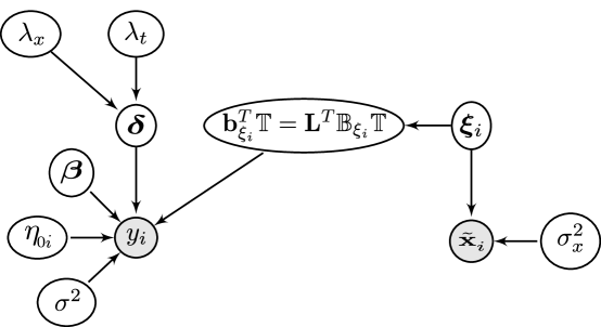
Figure 1: Directed Acyclic Graph for FGAM. Shaded vertices denote known quantities. The parameters $\{\nu_{m}\},\ \{\phi_{m}\},\ M,\text{ and }\mu_{x}$ are omitted since they are not updated by the VB algorithm.

For the optimal density for $\lambda_{x}$, we have from (8)

$$q^{*} (\lambda_{x})\propto\exp\mathopen{}\mathclose{{}\left[\operatorname{{{E}}}_{-\lambda_{x}}\{\log p(\lambda_{x}\mid\text{rest})\}}\right]$$

$$=\exp\mathopen{}\mathclose{{}\left[\operatorname{{{E}}}_{-\lambda_{x}}\mathopen{}\mathclose{{}\left\{\frac{1}{2}\log\lvert\lambda_{x}{\bm{\Psi}}_{x}+\lambda_{t}{\bm{\Psi}}_{t}\rvert-\frac{1}{2}{\bm{\delta}}^{T}(\lambda_{x}{\bm{\Psi}}_{x}){\bm{\delta}}+(a_{l}+1)\log(\lambda_{x})-b_{l}\lambda_{x}}\right\}}\right]$$

$$\approx\exp\mathopen{}\mathclose{{}\left[\frac{1}{2}\log\lvert\lambda_{x}{\bm{\Psi}}_{x}+{\mu_{q(\lambda_{t})}}{\bm{\Psi}}_{t}\rvert-\frac{\lambda_{x}}{2}\mathopen{}\mathclose{{}\left\{\text{tr}({\bm{\Psi}}_{x}{{\bm{\Sigma}}_{q({\bm{\delta}})}})+{\mu_{q({\bm{\delta}})}}^{T}{\bm{\Psi}}_{x}{\mu_{q({\bm{\delta}})}}}\right\}+(a_{l}+1)\log(\lambda_{x})-b_{l}\lambda_{x}}\right]$$

$$=\lvert\lambda_{x}{\bm{\Psi}}_{x}+{\mu_{q(\lambda_{t})}}{\bm{\Psi}}_{t}\rvert^{1/2}\exp\mathopen{}\mathclose{{}\left[-b_{l}\lambda_{x}-\frac{\lambda_{x}}{2}\mathopen{}\mathclose{{}\left\{\text{tr}({\bm{\Psi}}_{x}{{\bm{\Sigma}}_{q({\bm{\delta}})}})+{\mu_{q({\bm{\delta}})}}^{T}{\bm{\Psi}}_{x}{\mu_{q({\bm{\delta}})}}}\right\}}\right]\lambda_{x}^{a_{l}+1}\equiv{\widetilde{q}_{\lambda_{x}}(\lambda_{x})},$$ (9)

where the approximation comes from plugging in ${\mu_{q(\lambda_{t})}}$ for $\lambda_{t}$ to avoid taking an expectation of the determinant term over $\lambda_{t}$. Notice $c_{q(\lambda_{x})}\equiv\int_{0}^{\infty}{\widetilde{q}_{\lambda_{x}}({x})}\,dx$ has the form $c_{q(\lambda_{x})}=\int_{0}^{\infty}x^{a_{l}+1}e^{-x}f(x)\,dx$ which can be approximated by generalized Gauss-Laguerre quadrature. Using this type of quadrature for variational Bayes is discussed in [39] and is implemented in R in the package statmod [36], and we use it to determine a grid of $G$ points, ${\mathbf{g}}$, and quadrature weights, ${\mathbf{L}}_{g}$. Our approximations are then given by $c_{q(\lambda_{x})}\approx{\mathbf{L}}_{g}^{T}\widetilde{q}_{\lambda_{x}}({\mathbf{g}})$ and ${\mu_{q(\lambda_{x})}}\approx\{{\mathbf{L}}_{g}^{T}\widetilde{q}_{\lambda_{x}}({\mathbf{g}})\}^{-1}{\mathbf{L}}_{g}^{T}\mathopen{}\mathclose{{}\left\{{\mathbf{g}}\odot\widetilde{q}_{\lambda_{x}}({\mathbf{g}})}\right\}.$

Due to the exponential term in (9), moderate to large values of $\lambda_{x}$ result in $\widetilde{q}_{\lambda_{x}}(\lambda_{x})$ being evaluated to be zero, unless care is taken during the computation to avoid underflow. One strategy for avoiding loss of precision is as follows. Define $\ell_{\lambda_{x}}(x)=\log{\widetilde{q}_{\lambda_{x}}({x})}$ and $m_{\lambda_{x}}=\max_{\mathbf{g}}\ell_{\lambda_{x}}({\mathbf{g}})$, then $c_{q(\lambda_{x})}\approx\exp(m_{\lambda_{x}}){\mathbf{L}}_{g}^{T}\exp\{\ell_{\lambda_{x}}({\mathbf{g}})-m_{\lambda_{x}}\}$. The term $\exp(m_{\lambda_{x}})$ is in both the numerator and the denominator of ${\mu_{q(\lambda_{x})}}$ and thus drops out in that calculation. Taking the logarithm of the determinant in ${\widetilde{q}_{\lambda_{x}}(\lambda_{x})}$ is not a problem because ${\bm{\Psi}}_{x}$ and ${\bm{\Psi}}_{t}$ are diagonal.

For updating the principal component scores in our VB algorithm, recall the form of the full conditional

$$p({\bm{\xi}}_{i}\mid\text{rest})\propto p(y_{i}\mid\eta_{0i},{\bm{\beta}},{\bm{\delta}},{\bm{\xi}}_{i},\sigma^{2})p(\widetilde{{\mathbf{x}}}_{i}\mid{\bm{\xi}}_{i},\sigma^{2}_{x})p({\bm{\xi}}_{i})$$

$$\propto\exp\mathopen{}\mathclose{{}\left\{-\frac{1}{2\sigma^{2}}(y_{i}-\eta_{0i}-{{\mathbf{b}}_{{\bm{\xi}}_{i}}^{T}}{\bm{\theta}})^{2}}\right\}\exp\mathopen{}\mathclose{{}\left\{-\frac{1}{2\sigma_{x}^{2}}\mid\!\mid\widetilde{{\mathbf{x}}}_{i}-{\bm{\mu}}_{x}({\mathbf{t}}_{i})-{\bm{\Phi}}({\mathbf{t}}_{i}){\bm{\xi}}_{i}\mid\!\mid^{2}_{2}}\right\}\exp\mathopen{}\mathclose{{}\left\{-\frac{1}{2}{\bm{\xi}}_{i}^{T}\operatorname{{{diag}}}({\bm{\nu}}^{-1}){\bm{\xi}}_{i}}\right\},$$

where as before ${{\mathbf{b}}_{{\bm{\xi}}_{i}}^{T}}={\mathbf{L}}^{T}{\mathbb{B}}_{\xi_{i}}$ with ${\mathbb{B}}_{\xi_{i}}$ given by (5). We have,

$$\text{E}_{-{\bm{\xi}}_{i}} \mathopen{}\mathclose{{}\left\{-\frac{1}{2\sigma^{2}}(y_{i}-\eta_{0i}-{{\mathbf{b}}_{{\bm{\xi}}_{i}}^{T}}{\bm{\theta}})^{2}}\right\}=-\frac{{\mu_{q(1/\sigma^{2})}}}{2}\operatorname{{{E}}}_{-{\bm{\xi}}_{i}}\mathopen{}\mathclose{{}\left[\{y_{i}-\mu_{q(\eta_{0i})}-\operatorname{{{E}}}_{-{\bm{\xi}}_{i}}({{\mathbf{b}}_{{\bm{\xi}}_{i}}^{T}}{\bm{\theta}})\}^{2}}\right]$$

$$-\frac{1}{2}{\mu_{q(1/\sigma^{2})}}\sigma^{2}_{q(\eta_{0i})}-\frac{{\mu_{q(1/\sigma^{2})}}}{2}\operatorname{{{E}}}_{-{\bm{\xi}}_{i}}\mathopen{}\mathclose{{}\left\{({{\mathbf{b}}_{{\bm{\xi}}_{i}}^{T}}{\bm{\theta}}-\operatorname{{{E}}}_{-{\bm{\xi}}_{i}}({{\mathbf{b}}_{{\bm{\xi}}_{i}}^{T}}{\bm{\theta}}))^{2}}\right\}$$

$$=-\frac{{\mu_{q(1/\sigma^{2})}}}{2}\mathopen{}\mathclose{{}\left[(y_{i}-\mu_{q(\eta_{0i})}-{{\mathbf{b}}_{{\bm{\xi}}_{i}}^{T}}{\mu_{q({\bm{\theta}})}})^{2}+\sigma^{2}_{q(\eta_{0i})}+\operatorname{{{E}}}_{-{\bm{\xi}}_{i}}\mathopen{}\mathclose{{}\left\{({\bm{\theta}}-{\mu_{q({\bm{\theta}})}})^{T}{{\mathbf{b}}_{{\bm{\xi}}_{i}}}{{\mathbf{b}}_{{\bm{\xi}}_{i}}^{T}}({\bm{\theta}}-{\mu_{q({\bm{\theta}})}})}\right\}}\right]$$

$$=-\frac{{\mu_{q(1/\sigma^{2})}}}{2}\mathopen{}\mathclose{{}\left\{(y_{i}-\mu_{q(\eta_{0i})}-{{\mathbf{b}}_{{\bm{\xi}}_{i}}^{T}}{\mu_{q({\bm{\theta}})}})^{2}+\sigma^{2}_{q(\eta_{0i})}+\operatorname{tr}({{\mathbf{b}}_{{\bm{\xi}}_{i}}}{{\mathbf{b}}_{{\bm{\xi}}_{i}}^{T}}{{\bm{\Sigma}}_{q({\bm{\theta}})}})}\right\}$$

Therefore,

$$q^{*}({\bm{\xi}}_{i}) \propto\exp\mathopen{}\mathclose{{}\left[-\frac{{\mu_{q(1/\sigma^{2})}}}{2}\mathopen{}\mathclose{{}\left\{(y_{i}-\mu_{q(\eta_{0i})}-{{\mathbf{b}}_{{\bm{\xi}}_{i}}^{T}}{\mu_{q({\bm{\theta}})}})^{2}+\sigma^{2}_{q(\eta_{0i})}+\operatorname{tr}({{\mathbf{b}}_{{\bm{\xi}}_{i}}}{{\mathbf{b}}_{{\bm{\xi}}_{i}}^{T}}{{\bm{\Sigma}}_{q({\bm{\theta}})}})}\right\}}\right.$$

$$\qquad\mathopen{}\mathclose{{}\left.-\frac{{\mu_{q(1/\sigma_{x}^{2})}}}{2}\mid\!\mid\widetilde{{\mathbf{x}}}_{i}-{\bm{\mu}}_{x}({\mathbf{t}}_{i})-{\bm{\Phi}}({\mathbf{t}}_{i}){\bm{\xi}}_{i}\mid\!\mid^{2}_{2}-\frac{1}{2}{\bm{\xi}}_{i}^{T}\operatorname{{{diag}}}({\bm{\nu}}^{-1}){\bm{\xi}}_{i}}\right]$$

$$\propto\exp\mathopen{}\mathclose{{}\left[{\mu_{q(1/\sigma^{2})}}\{y_{i}-\mu_{q(\eta_{0i})}\}{{\mathbf{b}}_{{\bm{\xi}}_{i}}^{T}}{\mu_{q({\bm{\theta}})}}-\frac{{\mu_{q(1/\sigma^{2})}}}{2}\mathopen{}\mathclose{{}\left\{({{\mathbf{b}}_{{\bm{\xi}}_{i}}^{T}}{\mu_{q({\bm{\theta}})}})^{2}+{{\mathbf{b}}_{{\bm{\xi}}_{i}}^{T}}{{\bm{\Sigma}}_{q({\bm{\theta}})}}{{\mathbf{b}}_{{\bm{\xi}}_{i}}}}\right\}}\right.$$

$$\qquad\mathopen{}\mathclose{{}\left.+{\mu_{q(1/\sigma_{x}^{2})}}\{\widetilde{{\mathbf{x}}}_{i}-{\bm{\mu}}_{x}({\mathbf{t}}_{i})\}^{T}{\bm{\Phi}}({\mathbf{t}}_{i}){\bm{\xi}}_{i}-\frac{1}{2}{\bm{\xi}}_{i}^{T}\mathopen{}\mathclose{{}\left\{{\mu_{q(1/\sigma_{x}^{2})}}{\bm{\Phi}}^{T}({\mathbf{t}}_{i}){\bm{\Phi}}({\mathbf{t}}_{i})+\operatorname{{{diag}}}({\bm{\nu}}^{-1})}\right\}{\bm{\xi}}_{i}}\right]\equiv q({\bm{\xi}}_{i}).$$

Since this does not have the form of a standard, known density, we will employ a Laplace approximation. The use of Laplace approximations for variational inference with nonconjugate models was also explored in [40]. This is given by

$$q^{*}({\bm{\xi}}_{i})=N({\bm{\xi}}_{i,0},{\bm{\Lambda}}_{i}^{-1})\quad\text{where}\quad{\bm{\Lambda}}_{i}=\mathopen{}\mathclose{{}\left.-{\mathcal{D}}_{{\bm{\xi}}_{i}^{T}}{\mathcal{D}}_{{\bm{\xi}}_{i}}\log q({\bm{\xi}}_{i})}\right|_{{\bm{\xi}}_{i}={\bm{\xi}}_{i,0}},$$ (10)

with ${\mathcal{D}}_{\mathbf{a}}[\cdot]$ denoting differentiation w.r.t. the vector ${\mathbf{a}}$ and ${\bm{\xi}}_{i,0}$ denoting the mode of $q^{*}({\bm{\xi}}_{i})$, which is found by a numerical optimization routine. The formula for ${\bm{\Lambda}}_{i}$ is given in Appendix B. We expect the Laplace approximation to perform well in high sparsity settings because the Gaussian prior becomes the dominant part of the posterior in these situations.

To construct our algorithm, we also require the expectation of ${{\mathbf{b}}_{{\bm{\xi}}_{i}}}$ and the expectation of its outer product with respect to ${\bm{\xi}}_{i}$. To do this we use second-order Taylor expansions about ${\bm{\xi}}_{i,0}$. These derivations are also left to Appendix B. Our log-likelihood lower bound, which is used for monitoring convergence of our algorithm, is derived in Appendix C and the full variational Bayes algorithm is given in Appendix D as Algorithm 2.

6 Simulation Study

We now conduct a simulation study to compare the efficacy of our proposed approaches. We fit each model to 100 simulated data sets. The true functional covariates are given by $X(t)=\sum_{j=1}^{4}\xi_{j}\phi_{j}(t),$ with $\xi_{j}\sim N(0,8j^{-2})$ and $\{\phi_{1}(t),\ldots,\phi_{4}(t)\}=\{\sin(\pi t/\lvert{\mathcal{T}}\rvert),\cos(\pi t/\lvert{\mathcal{T}}\rvert),\sin(2\pi t/\lvert{\mathcal{T}}\rvert),\cos(2\pi t/\lvert{\mathcal{T}}\rvert)\}$, with $\rvert{\mathcal{T}}\lvert$ denoting the measure of the interval ${\mathcal{T}}$. To examine how our model performs with both sparse and dense but irregularly observed data, we generate observed covariates by randomly selecting $J_{i}=10$ or $J_{i}=40$ points for each subject from a grid of 50 equally-space points used to generate the true response. We consider three different levels of the measurement error variance, $\sigma_{x}^{2}=0,1,\text{ and }4$. The response error variance is taken to be $\sigma^{2}=1$. We examine two different possibilities for the regression surface $F(x,t)$. First, a case where the FLM is the true model, $F(x,t)=2x\sin(\pi t)$, with ${\mathcal{T}}=[0,1]$; and next, a case where the FLM does not hold, $F(x,t)=20\cos\mathopen{}\mathclose{{}\left(-\frac{x}{8}+\frac{t}{4}-5}\right)$, with ${\mathcal{T}}=[0,10]$. A sampling of some generated curves including measurement error for both levels of sparsity as well as plots of both true surfaces can be found in Figure 2.

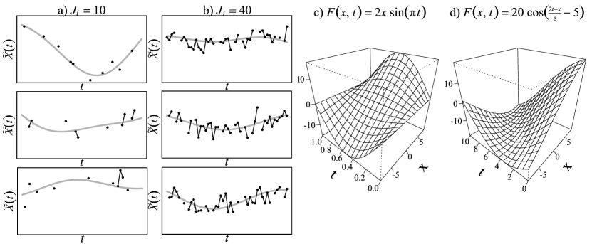
Figure 2: Plots a) and b) show three observed functional predictors for varying levels of sparsity when $\sigma_{x}=1$. The true trajectories are also plotted in grey. Plot c) shows the surface $F(x,t)=2x\sin(\pi t)$ and plot d) the surface $F(x,t)=20\cos\mathopen{}\mathclose{{}\left(-\frac{x}{8}+\frac{t}{4}-5}\right)$.

For our comparison we consider seven different methods for fitting FLMs and FGAMs: 1) a baseline/oracle FGAM fit by the [24] approach when the fully observed curves without measurement error are known (trueX), 2) FGAM fit by [24] with fixed trajectories estimated using the procedure outlined in Section 2 (PACE), 3) FGAM fit using variational Bayes on the sparse, noisy curves (VB), 4) FGAM fit using MCMC and the sparse, noisy curves (MCMC), 5) as in 4) except initial values are supplied by the VB fit (VB-MCMC), 6) FLM fit using penalized splines with trajectories obtained from the Section 2 procedure (FLM-PACE), and 7) FLM fit to the fully observed curves without measurement error (FLMtrueX). Each method used cubic B-splines and second-order difference penalties. The [24] implementation of FGAM is fit using their code which is available in the package refund [4] in R [30]. Smoothing parameters are chosen by generalized cross validation (GCV) using the package mgcv [45], which is also used to estimate the FLMs. MCMC runs one chain for 10,000 iterations after a burn-in of 1000, whereas VB-MCMC uses only 1000 iterations after a burn-in of 500. Each method uses and, if applicable, estimates exactly the true number of non-zero components $M=4$. For each simulated data set, we use two thirds of the 100 observations to fit the models and the other one third for prediction.

We first compare how well PACE, VB, MCMC, and VB-MCMC do at estimating the functional covariates. The median over simulations of the in-sample root mean integrated square error, ${\text{RMISE-X}}^{2}=N^{-1}\sum_{i=1}^{67}\int_{{\mathcal{T}}}\{X_{i}(t)-\widehat{X}_{i}(t)\}^{2}\,dt$, for each scenario and method is reported in Figure 3 a). We see that the PACE method does not perform well in the sparse data scenarios $(J_{i}=10)$. One reason for this is that it does not account for the variability from imputing the principal component scores. An additional reason is difficulties in estimating a covariance matrix for the functional predictors. The estimate is often singular or near-singular and this causes numerical problems when attempting to estimate all four non-zero principal component scores using the method presented in Section 2. Our Bayesian algorithms do not suffer from this problem even when starting from poorly conditioned initial estimates from our PACE implementation. We see that VB performs quite well at recovering the trajectories, even in the $J_{i}=10$ scenarios. MCMC performs slightly worse than VB here. Further investigation showed that MCMC on average slightly overestimated $\sigma_{x}^{2}$ which made it less accurate for in-sample recovery, but that this added variance made for more accurate prediction of trajectories out-of-sample. The observed acceptance rates for the independent Metropolis-Hastings step used to update the principal component scores were consistently above 0.9 for all scenarios indicating that our proposal distribution performed well for this data.

Figure 3: a) Median RMISE over 100 simulations for two levels of sparsity and different values for the measurement error variance for recovering in-sample trajectories, $X(t)$. b) Median RISE for predicting the true surface, $F(x,t)$. b) includes trueX which is not relevant for a). Values that do not fall within the y-axis limits are individually labeled.

Now turning to estimation of the true surface $F(x,t)$, we report the median root integrated square error, RISE-F${}^{2}=\int_{\mathcal{X}}\int_{\mathcal{T}}\mathopen{}\mathclose{{}\left\{F(x,t)-\widehat{F}(x,t)}\right\}^{2}\,dt\,dx$, in Figure 3 b). We evaluate the RISE only at $(x,t)$ values that are inside the convex hull defined by the observed trajectories for that sample to avoid regions of the plane where there are no data. We again observe performance from the PACE method to be poor in the sparse settings. Interestingly, the MCMC and MCMC-VB approaches have lower ISE than the trueX method. We suspect this is due to the MCMC algorithm on average choosing larger smoothing parameters which are closer to the optimal values for smoothing the surface than those chosen by GCV for the trueX fits. Due to the additional smoothing performed by the integration in (2), the optimal amount of smoothing for estimating the response and for estimating the surface are different [3]. Also noteworthy is the substantial difference between VB and MCMC depending on the true regression surface. This again seems to be due to differences in how the smoothing parameters are chosen.

Finally, results for root mean square error (RMSE) for predicting the out-of-sample response, $\text{RMSE-Y}^{2}=\frac{1}{33}\sum_{i=68}^{100}(Y_{i}-\widehat{Y}_{i})^{2}$, can be found in Figure 4. We see that the performance of MCMC matches and even sometimes outperforms the oracle trueX method that knows the entire trajectories. Overall, we recommend the combination of VB for initial estimates followed by MCMC as it appears to be best or close to best in nearly all scenarios. The total elapsed time for estimating FGAM on one data set averaged over all simulations and scenarios was 43.3 seconds for VB, 732.0 seconds for MCMC, and 153.5 seconds for VB-MCMC.

Figure 4: Median RMSE over 100 simulations for out-of-sample predictions of the response, $Y$, for two levels of sparsity and different values for the measurement error variance. Values that do not fall within the y-axis limits are individually labeled

7 Analysis of Auction Data

In this section we fit our proposed models to auction data from the online auction website eBay and attempt to forecast closing auction price. The data set contains the time and amount of every bid for 155 seven-day auctions of Palm M515 Personal Digital Assistants (PDA) that took place between March and May, 2003. Each auction is "standardized" to start at time 0. This data was previously analyzed using functional data methods in a series of work by W. Jank, G. Shmueli and coauthors [19, 42, e.g.,]. The PACE methodology introduced in Section 2 was used to analyze this data set in [22]. Typically, each auction consists of three clearly discernible parts: an initial period with some bidding, a middle period with very few bids, and a final period of rapid bidding as the auction finishes [42]. This sparsity and irregularity in the observed bid data means that the usual methods of function data analysis are not appropriate.

Our raw data is actually the maximum amount the bidder is willing to pay for the item, often called the willing-to-pay (WTP) value. To recover the current item price from the WTP values, we must use the table available at http://pages.ebay.com/help/buy/bid-increments.html. When a new WTP value is entered that is more than any previous WTP value, the new price is determined by incrementing the current price in an amount given by this table. A new bidder must enter an amount at least as large as this new price plus the increment given by the table. We assume there is an underlying smooth price process that we attempt to recover with our proposed approaches.

We use the logarithm of the ratio of successive prices during the first six days of the auction to predict the logarithm of the closing price on the final day. Hourly prices are used so that we are trying to recover $6\times 24=144$ prices for each auction. When an auction has multiple bids in the same hour, we take the average of the prices corresponding to those bids as the observed price for that hour. As in [22], we set any negative values for the log-price ratio equal to zero, which can occur because initial log-price at time $0$ is taken to be zero. To show the usefulness of our MCMC and VB methods, we fit the FGAM and FLM using the trajectory of observed log-price ratios, log$\{\widetilde{x}_{i}(t_{i,j})/\widetilde{x}_{i}(t_{i,j-1})\}$, for the first six days in order to predict the logarithm of the final selling price at the end of the seventh day. We emphasize that no information on the prices from the final day of the auction are included in the functional predictor so that we have a true measure of forecasting accuracy.

We randomly partition the data into training and test sets with two thirds of the samples used for training and one third for testing. We compute the root mean square error (RMSE) for predicting the logarithm of the closing price for the test data set after fitting each model to the training data. This is repeated for 25 different splits into test and training sets. For comparison, we also considered the simple two-step approach of using PACE to recover the functional predictors and then using these estimates to fit FLMs and FGAMs in refund as in the fully-observed predictor case from [24]. For the FGAM methods, ten basis functions were used for both axes.

The surface estimated by our MCMC algorithm fit to the entire data set is displayed in Figure 5 b) along with the observed and estimated log-price ratios for five randomly chosen auctions. Figure 5 a) plots all estimated trajectories and additionally histograms showing the frequencies of observations for both $X(t)$ and $t$; notice from the histogram on the right part of the plot that the majority of the data is grouped at very low log-price ratios. In b) we see that large values of the log-price ratio in the early hours of the auction result in a lower predicted value for the closing price and that smaller ratios later towards the end of the sixth day of the auction result in higher predicted closing price. Nonlinearities in the log-price component of the estimated surface suggest that an FLM may not be flexible enough for this data set. There appears to be some undersmoothing of the functional predictors in Figure 5 a). [3] showed that for optimal prediction in the FLM, the coefficient function should be undersmoothed because of the additional smoothing performed by the integral in the regression function. We conjecture that some degree of undersmoothing of the functional predictors is desirable for our forecasting problem when estimating (6) for similar reasons.

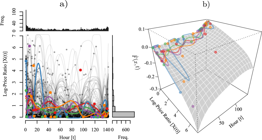
Figure 5: a) All estimated trajectories from use of our MCMC algorithm on the auction data with points representing observed data. Five trajectories are highlighted and also plotted in b). Also included are two histograms showing which covariate values occur with the highest frequency (on the right) and the frequency of bids for each hour of the auction (on top). b) Shows the estimated surface $\widehat{F}(x,t)$ from fitting FGAM to the auction data using MCMC. The overlayed points and curves are the same as a)

The median out-of-sample RMSE over 25 partitions of the data is reported in Table 1 along with standard deviations. We can see that our Bayesian approach for fitting FGAM offers the best performance in this case, with both FGAM-MCMC and FGAM-VB offering much improved performance over the methods that only use PACE followed by estimation of FGAM in refund. Both methods that simply used PACE and then assumed fully observed data had very poor performance for some of the splits when the imputed trajectories were especially bad.

FLM-PACE	FGAM-PACE	FGAM-MCMC	FGAM-VB
0.5917(1.3093)	4.913(0.4322)	0.0914(0.0052)	0.0905(0.0037)

Table 1: Median RMSE (with standard deviation in parentheses) for out of sample predictions of log-final selling price for 25 random splits of the auction data

8 Conclusion

We have proposed two algorithms for fitting a nonlinear regression model for scalar on function regression when the functional predictor is sparsely observed with measurement error. After first expressing the FGAM as a linear mixed model with missing data, we then took a Bayesian hierarchical modeling approach and fit our model using a Metropolis-within-Gibbs sampler. Our MCMC algorithm was able to provide useful inferences in difficult situations where initial estimates provided by standard FPCA methods were quite poor due to rank deficiency in the estimated covariance matrix.

Additionally, we developed a variational Bayesian algorithm for fitting FGAM which can be used to quickly obtain approximate parameter estimates. We demonstrated the usefulness of our approach using simulated data and an application to a longitudinal data set involving online auctions. We developed a Laplace approximation that accurately approximated the intractable optimal density for the principal component scores. We also demonstrated the usefulness of using the estimates from our VB algorithm as inputs to the MCMC algorithm to obtain faster convergence.

An alternative way to account for uncertainty in the imputed trajectories would be using the bootstrap approach of [13]. We did implement this method, but due to space concerns, we have not included it in this work. In our experiments, this approach did not perform as well as our Bayesian algorithms and was slower than the combined VB-MCMC approach.

An interesting area for future work brought up by a referee is that of using the estimates from a VB algorithm in a more principled way to achieve faster convergence of an MCMC algorithm than the simple approach considered in this work of using the VB estimates as starting values for the MCMC. Naively using a variational approximate distribution as a proposal density or as a prior distribution in a MCMC algorithm could be problematic due to the tendency for variational Bayes to underestimate the true variance. [6] demonstrated some algorithms combining MFVB and MCMC that attempted to deal with this issue. Additional areas for future work include investigating coverage for credible bands provided by our variational Bayes algorithm and comparing with credible intervals from MCMC. Typically, credible bands derived from variational Bayes procedures suffer from undercoverage. Bootstrapping the estimates from our variational Bayes algorithm may be a promising way around this issue [14]. Another promising approach for correcting covariance estimates from MFVB was recently proposed in [11]. We are also working on extensions to the case of functional responses and binary responses.

Appendix Appendix A Derivation of Full Conditional Distributions

In this appendix we derive the full conditional distributions for the variance components and spline coefficients in (6) and also give the full posterior distribution.

Variance parameters

We begin by defining the $N\times d_{x}d_{t}$ matrix ${\mathbb{Z}}_{0}$ whose $i$th row is given by ${\mathbf{Z}}_{0,i}^{T}={\mathbf{L}}^{T}{\mathbb{B}}_{\xi_{i}}{\mathbb{T}}_{0}={{\mathbf{b}}_{{\bm{\xi}}_{i}}^{T}}{\mathbb{T}}_{0}$ and the $N\times(K_{x}K_{t}-d_{x}d_{t})$ matrix ${\mathbb{Z}}_{p}$ with $i$th row given by ${\mathbf{Z}}_{p,i}^{T}={{\mathbf{b}}_{{\bm{\xi}}_{i}}^{T}}{\mathbb{T}}_{p}$. We also define ${\mathbf{y}}_{\eta_{0}}=(y_{1}-\eta_{0,1},\ldots,y_{N}-\eta_{0,N})^{T}$, $\bm{\eta}_{1}={\mathbb{Z}}_{0}{\bm{\beta}}+{\mathbb{Z}}_{p}{\bm{\delta}}$ with $i$th component $\eta_{1,i}={{\mathbf{b}}_{{\bm{\xi}}_{i}}^{T}}\{{\mathbb{T}}({\bm{\beta}}^{T},{\bm{\delta}}^{T})^{T}\}={{\mathbf{b}}_{{\bm{\xi}}_{i}}^{T}}{\mathbb{T}}_{0}{\bm{\beta}}+{{\mathbf{b}}_{{\bm{\xi}}_{i}}^{T}}{\mathbb{T}}_{p}{\bm{\delta}},$, and ${\bm{\Xi}}=[{\bm{\xi}}_{1}:\cdots:{\bm{\xi}}_{N}]^{T}$, we have

$$p(\sigma^{2}\mid\cdot) \propto p({\mathbf{y}}\mid\eta_{0,1},\ldots,\eta_{0,N},{\bm{\beta}},{\bm{\delta}},\sigma^{2},{\bm{\Xi}})p(\sigma^{2})$$

$$\propto(\sigma^{2})^{-N/2-a_{s}-1}\exp\mathopen{}\mathclose{{}\left\{-\frac{b_{s}+\frac{1}{2}\mathopen{}\mathclose{{}\left({\mathbf{y}}_{\eta_{0}}-\bm{\eta}_{1}}\right)^{T}\mathopen{}\mathclose{{}\left({\mathbf{y}}_{\eta_{0}}-\bm{\eta}_{1}}\right)}{\sigma^{2}}}\right\}$$

$$\text{so that }\sigma^{2}\mid\cdot \sim\text{IG}\mathopen{}\mathclose{{}\left(a=N/2+a_{s},b=b_{s}+\frac{1}{2}\{{\mathbf{y}}_{\eta_{0}}-\bm{\eta}_{1}\}^{T}\{{\mathbf{y}}_{\eta_{0}}-\bm{\eta}_{1}\}}\right)$$

Similarly,

$$\sigma_{x}^{2}\mid\cdot \sim\text{IG}\mathopen{}\mathclose{{}\left(a=\sum^{N}_{i}n_{i}/2+a_{x},b=b_{x}+\frac{1}{2}\sum^{N}_{i}\sum_{j}^{n_{i}}\mathopen{}\mathclose{{}\left\{\widetilde{x}_{ij}-\mu_{x}(t_{ij})-\sum^{M}_{m}\phi_{m}(t_{ij})\xi_{im}}\right\}^{2}}\right).$$

Spline coefficients $\beta,{\bm{\delta}}$

$$p({\bm{\beta}},{\bm{\delta}}\mid\cdot) \propto p({\bm{\beta}})p({\bm{\delta}}\mid\lambda_{x},\lambda_{t})p(\lambda_{x})p(\lambda_{t})$$

$$\propto\exp\mathopen{}\mathclose{{}\left\{-\frac{({\mathbf{y}}-\bm{\eta}_{0}-{\mathbb{Z}}_{0}{\bm{\beta}}-{\mathbb{Z}}_{p}{\bm{\delta}})^{T}({\mathbf{y}}-\bm{\eta}_{0}-{\mathbb{Z}}_{0}{\bm{\beta}}-{\mathbb{Z}}_{p}{\bm{\delta}})}{2\sigma^{2}}}\right\}\exp\mathopen{}\mathclose{{}\left\{-\frac{1}{2}{\bm{\delta}}^{T}(\lambda_{x}{\bm{\Psi}}_{x}+\lambda_{t}{\bm{\Psi}}_{t}){\bm{\delta}}}\right\}$$

i.e.

$${\bm{\delta}}\mid\cdot \sim N({\mathbf{m}}_{b},{\mathbb{S}}_{b})\text{ with }$$

$${\mathbb{S}}_{b} =({\mathbb{Z}}_{p}^{T}{\mathbb{Z}}_{p}/\sigma^{2}+\lambda_{x}{\bm{\Psi}}_{x}+\lambda_{t}{\bm{\Psi}}_{t})^{-1},$$

$${\mathbf{m}}_{b} ={\mathbb{S}}_{b}{\mathbb{Z}}_{p}^{T}\mathopen{}\mathclose{{}\left({\mathbf{y}}_{\eta_{0}}-{\mathbb{Z}}_{0}{\bm{\beta}}}\right)/\sigma^{2};$$

$${\bm{\beta}}\mid\cdot \sim N({\mathbf{m}}_{\beta},{\mathbb{S}}_{\beta})\text{ with }$$

$${\mathbb{S}}_{\beta} =({\mathbb{Z}}_{0}^{T}{\mathbb{Z}}_{0}/\sigma^{2})^{-1},$$

$${\mathbf{m}}_{\beta} ={\mathbb{S}}_{\beta}{\mathbb{Z}}_{0}^{T}\mathopen{}\mathclose{{}\left({\mathbf{y}}_{\eta_{0}}-{\mathbb{Z}}_{p}{\bm{\delta}}}\right)/\sigma^{2}.$$

The full posterior distribution is given by

$$p({\bm{\beta}},{\bm{\delta}}, \sigma^{2},\lambda_{x},\lambda_{t},{\bm{\Xi}},\sigma^{2}_{x}\mid{\mathbf{y}},\widetilde{{\mathbf{x}}},\eta_{0,1},\ldots,\eta_{0,N},{\bm{\mu}}_{x},{\bm{\Phi}},{\bm{\nu}})\propto$$

$$\propto(\sigma^{2})^{-N/2}\exp\mathopen{}\mathclose{{}\left[-\frac{1}{2\sigma^{2}}\sum_{i}^{N}\mathopen{}\mathclose{{}\left\{y_{\eta_{0},i}-\sum^{K_{x}}_{j=1}\sum^{K_{t}}_{k=1}{\mathbf{L}}^{T}\mathopen{}\mathclose{{}\left[{\mathbf{B}}^{\mathcal{X}}_{j}\mathopen{}\mathclose{{}\left({\bm{\mu}}_{x}+{\bm{\Phi}}{\bm{\xi}}_{i}}\right)\cdot{\mathbf{B}}^{\mathcal{T}}_{k}({\mathbf{t}})}\right][{\mathbb{T}}({\bm{\beta}}^{T},{\bm{\delta}}^{T})^{T}]_{j,k}}\right\}^{2}}\right]\cdot$$

$$\quad\cdot(\sigma_{x}^{2})^{-\sum^{N}_{i}n_{i}/2}\exp\mathopen{}\mathclose{{}\left[-\frac{1}{2\sigma_{x}^{2}}\sum_{i}^{N}\lvert\widetilde{{\mathbf{x}}}_{i}-\mu_{x}({\mathbf{t}}_{i})-{\bm{\Phi}}({\mathbf{t}}_{i}){\bm{\xi}}_{i}\rvert^{2}_{2}}\right]\cdot$$

$$\quad\cdot\lvert\lambda_{x}{\bm{\Psi}}_{x}+\lambda_{t}{\bm{\Psi}}_{t}\rvert^{1/2}\exp\mathopen{}\mathclose{{}\left(-\frac{1}{2}{\bm{\delta}}^{T}(\lambda_{x}{\bm{\Psi}}_{x}+\lambda_{t}{\bm{\Psi}}_{t}){\bm{\delta}}}\right)\cdot$$

$$\quad\cdot\exp\mathopen{}\mathclose{{}\left(-\frac{1}{2}\sum_{i}^{N}{\bm{\xi}}_{i}^{T}\operatorname{{{diag}}}({\bm{\nu}}^{-1}){\bm{\xi}}_{i}}\right)\cdot(\sigma^{2})^{-a_{s}-1}\exp(-b_{s}/\sigma^{2})\cdot(\sigma_{x}^{2})^{-a_{x}-1}\exp(-b_{x}/\sigma_{x}^{2})\cdot$$

$$\quad\cdot(\lambda_{x})^{a_{l}+1}\exp(-b_{l}\lambda_{x})(\lambda_{t})^{a_{l}+1}\exp(-b_{l}\lambda_{t}),$$

where $[{\mathbb{A}}]_{j,k}$ denotes the entry in the $j$th row and $k$th column of the matrix ${\mathbb{A}}$.

Appendix Appendix B Derivation Of Optimal Proposal Densities

In this section we derive the optimal densities, $q^{*}$, for parameters that were given conjugate priors and give detailed calculations for our Laplace approximation to the optimal density for the principal component scores. We use the notation and full conditionals from Appendix A and often make use of the results that for ${\mathbf{x}}\sim({\bm{\mu}},{\bm{\Sigma}}),\ \operatorname{{{E}}}[{\mathbf{x}}^{T}{\mathbf{S}}{\mathbf{x}}]=\operatorname{tr}({\mathbf{S}}{\bm{\Sigma}})+{\bm{\mu}}^{T}{\mathbf{S}}{\bm{\mu}}\text{ and }\operatorname{{{E}}}[{\mathbf{x}}{\mathbf{x}}^{T}]=\operatorname{{{E}}}[{\mathbf{x}}]\operatorname{{{E}}}[{\mathbf{x}}]^{T}+\operatorname{{{var}}}[{\mathbf{x}}].$

We first discuss the updates for the offset terms, $\eta_{0i}$, $i=1,\ldots,N$. For simplicity, we assume that they can be expressed as $\eta_{0i}={\mathbf{u}}_{i}^{T}\bm{\eta}_{0}$ or ${(\eta_{01},\ldots,\eta_{0N})^{T}={\mathbb{U}}\bm{\eta}_{0}}$, where ${\mathbb{U}}$ is an $N\times p_{0}$ matrix with rows ${\mathbf{u}}_{i}^{T}$ containing, for e.g., scalar covariate observations for parametric terms, basis function evaluations for nonparametric terms, or a leading column of ones for an intercept. Further generalizations are straightforward. The coefficient vector $\bm{\eta}_{0}$ has prior density $p(\bm{\eta}_{0})=N(\mathbf{0},\sigma^{2}_{\bm{\eta}_{0}}{\mathbb{I}}_{p_{0}}),$ with $\sigma^{2}_{\bm{\eta}_{0}}$ large and fixed. The full conditional is given by

$$p(\bm{\eta}_{0}\mid\text{rest}) \propto p({\mathbf{y}}\mid\bm{\eta}_{0},{\bm{\beta}},{\bm{\delta}},{\bm{\Xi}},\sigma^{2})p(\bm{\eta}_{0})\propto\exp\mathopen{}\mathclose{{}\left[-\frac{({\mathbf{y}}-{\mathbb{U}}\bm{\eta}_{0}-\bm{\eta}_{1})^{T}({\mathbf{y}}-{\mathbb{U}}\bm{\eta}_{0}-\bm{\eta}_{1})}{2\sigma^{2}}-\frac{1}{\sigma^{2}_{\bm{\eta}_{0}}}\bm{\eta}_{0}^{T}{\mathbb{I}}_{p_{0}}\bm{\eta}_{0}}\right]$$

$$\propto\exp\mathopen{}\mathclose{{}\left\{-\frac{1}{2}\mathopen{}\mathclose{{}\left[\bm{\eta}_{0}^{T}\mathopen{}\mathclose{{}\left(\frac{1}{\sigma^{2}}{\mathbb{U}}^{T}{\mathbb{U}}+\frac{1}{\sigma^{2}_{\bm{\eta}_{0}}}{\mathbb{I}}_{p_{0}}}\right)\bm{\eta}_{0}-2\mathopen{}\mathclose{{}\left(({\mathbf{y}}-\bm{\eta}_{1})^{T}{\mathbb{U}}/\sigma^{2}}\right)\bm{\eta}_{0}}\right]}\right\}.$$

Thus,

$$q^{*}(\bm{\eta}_{0}) \propto\exp\mathopen{}\mathclose{{}\left\{-\frac{1}{2}\operatorname{{{E}}}_{-\bm{\eta}_{0}}\mathopen{}\mathclose{{}\left[\bm{\eta}_{0}^{T}\mathopen{}\mathclose{{}\left(\frac{1}{\sigma^{2}}{\mathbb{U}}^{T}{\mathbb{U}}+\frac{1}{\sigma^{2}_{\bm{\eta}_{0}}}{\mathbb{I}}_{p_{0}}}\right)\bm{\eta}_{0}-2\mathopen{}\mathclose{{}\left(({\mathbf{y}}-\bm{\eta}_{1})^{T}{\mathbb{U}}/\sigma^{2}}\right)\bm{\eta}_{0}}\right]}\right\}$$

$$\propto\exp\mathopen{}\mathclose{{}\left\{-\frac{1}{2}\mathopen{}\mathclose{{}\left[\bm{\eta}_{0}^{T}\mathopen{}\mathclose{{}\left({\mu_{q(1/\sigma^{2})}}{\mathbb{U}}^{T}{\mathbb{U}}+\frac{1}{\sigma^{2}_{\bm{\eta}_{0}}}{\mathbb{I}}_{p_{0}}}\right)\bm{\eta}_{0}-2\mathopen{}\mathclose{{}\left(({\mathbf{y}}-{\mu_{q(\bm{\eta}_{1})}})^{T}{\mathbb{U}}{\mu_{q(1/\sigma^{2})}}}\right)\bm{\eta}_{0}}\right]}\right\},$$

where ${\mu_{q(\bm{\eta}_{1})}}={\mu_{q({\mathbf{b}}_{{\bm{\xi}}})}}{\mathbb{T}}({\mu_{q({\bm{\beta}})}}^{T},{\mu_{q({\bm{\delta}})}}^{T})^{T}$. Denote the rows of the $N\times K_{x}K_{t}$ matrix, ${\mu_{q({\mathbf{b}}_{{\bm{\xi}}})}}$, by ${\mu^{T}_{q({\mathbf{b}}_{{\bm{\xi}}_{i}})}}$. By completing the square, we see $q^{*}(\bm{\eta}_{0})=N({\mu_{q(\bm{\eta}_{0})}},{{\bm{\Sigma}}_{q(\bm{\eta}_{0})}})$ where ${{\bm{\Sigma}}_{q(\bm{\eta}_{0})}}=\mathopen{}\mathclose{{}\left({\mu_{q(1/\sigma^{2})}}{\mathbb{U}}^{T}{\mathbb{U}}+\frac{1}{\sigma^{2}_{\bm{\eta}_{0}}}{\mathbb{I}}_{p_{0}}}\right)^{-1}$ and ${\mu_{q(\bm{\eta}_{0})}}={{\bm{\Sigma}}_{q(\bm{\eta}_{0})}}{\mathbb{U}}^{T}({\mathbf{y}}-{\mu_{q(\bm{\eta}_{1})}}){\mu_{q(1/\sigma^{2})}}$.

Next, for ${\bm{\beta}}$

$$p({\bm{\beta}}\mid\text{rest}) \propto p({\mathbf{y}}\mid\bm{\eta}_{0},{\bm{\beta}},{\bm{\delta}},{\bm{\Xi}},\sigma^{2})p({\bm{\beta}})\propto\exp\mathopen{}\mathclose{{}\left[-\frac{({\mathbf{y}}-{\mathbb{U}}\bm{\eta}_{0}-\bm{\eta}_{1})^{T}({\mathbf{y}}-{\mathbb{U}}\bm{\eta}_{0}-\bm{\eta}_{1})}{2\sigma^{2}}-\frac{1}{\sigma^{2}_{{\bm{\beta}}}}{\bm{\beta}}^{T}{\mathbb{I}}_{d_{x}d_{t}}{\bm{\beta}}}\right]$$

$$\propto\exp\mathopen{}\mathclose{{}\left\{-\frac{1}{2}\mathopen{}\mathclose{{}\left[{\bm{\beta}}^{T}\mathopen{}\mathclose{{}\left(\frac{1}{\sigma^{2}}{\mathbb{Z}}_{0}^{T}{\mathbb{Z}}_{0}+\frac{1}{\sigma^{2}_{{\bm{\beta}}}}{\mathbb{I}}_{d_{x}d_{t}}}\right){\bm{\beta}}-2\mathopen{}\mathclose{{}\left(({\mathbf{y}}-{\mathbb{U}}\bm{\eta}_{0}-{\mathbb{Z}}_{p}{\bm{\delta}})^{T}{\mathbb{Z}}_{0}/\sigma^{2}}\right){\bm{\beta}}}\right]}\right\}$$

Thus,

$$q^{*}({\bm{\beta}}) \propto\exp\mathopen{}\mathclose{{}\left\{-\frac{1}{2}\mathopen{}\mathclose{{}\left[{\bm{\beta}}^{T}\mathopen{}\mathclose{{}\left({\mu_{q(1/\sigma^{2})}}\operatorname{{{E}}}_{-{\bm{\beta}}}[{\mathbb{Z}}_{0}^{T}{\mathbb{Z}}_{0}]+\frac{1}{\sigma^{2}_{{\bm{\beta}}}}{\mathbb{I}}_{d_{x}d_{t}}}\right){\bm{\beta}}}\right]}\right\}\cdot$$

$$\times\exp\mathopen{}\mathclose{{}\left\{-\frac{{\mu_{q(1/\sigma^{2})}}}{2}\mathopen{}\mathclose{{}\left[({\mathbf{y}}-{\mathbb{U}}{\mu_{q(\bm{\eta}_{0})}})^{T}{\mu_{q({\mathbf{b}}_{{\bm{\xi}}})}}{\mathbb{T}}_{0}-{\mu_{q({\bm{\delta}})}}^{T}\operatorname{{{E}}}_{-{\bm{\beta}}}({\mathbb{Z}}_{p}^{T}{\mathbb{Z}}_{0})}\right]{\bm{\beta}}}\right\},$$

where

$$\operatorname{{{E}}}({\mathbb{Z}}_{j}^{T}{\mathbb{Z}}_{k}) =\operatorname{{{E}}}\mathopen{}\mathclose{{}\left[\sum_{i=1}^{N}({\mathbb{T}}_{j}^{T}{{\mathbf{b}}_{{\bm{\xi}}_{i}}})({{\mathbf{b}}_{{\bm{\xi}}_{i}}^{T}}{\mathbb{T}}_{k})}\right]={\mathbb{T}}_{j}^{T}\mathopen{}\mathclose{{}\left[\sum_{i=1}^{N}\operatorname{{{E}}}_{{\bm{\xi}}}({{\mathbf{b}}_{{\bm{\xi}}_{i}}}{{\mathbf{b}}_{{\bm{\xi}}_{i}}^{T}})}\right]{\mathbb{T}}_{k},\qquad j,k=0,p.$$

Thus, $q^{*}({\bm{\beta}})=N({\mu_{q({\bm{\beta}})}},{{\bm{\Sigma}}_{q({\bm{\beta}})}})$ with

$${{\bm{\Sigma}}_{q({\bm{\beta}})}} =\mathopen{}\mathclose{{}\left\{{\mathbb{T}}_{0}^{T}\mathopen{}\mathclose{{}\left[\sum_{i=1}^{N}\operatorname{{{E}}}_{{\bm{\xi}}}\mathopen{}\mathclose{{}\left({{\mathbf{b}}_{{\bm{\xi}}_{i}}}{{\mathbf{b}}_{{\bm{\xi}}_{i}}^{T}}}\right)}\right]{\mathbb{T}}_{0}{\mu_{q(1/\sigma^{2})}}+\frac{1}{\sigma^{2}_{{\bm{\beta}}}}{\mathbb{I}}_{d_{x}d_{t}}}\right\}^{-1}$$

$${\mu_{q({\bm{\beta}})}} ={{\bm{\Sigma}}_{q({\bm{\beta}})}}{\mathbb{T}}_{0}^{T}\mathopen{}\mathclose{{}\left\{{\mu^{T}_{q({\mathbf{b}}_{{\bm{\xi}}})}}({\mathbf{y}}-{\mathbb{U}}{\mu_{q(\bm{\eta}_{0})}})-\mathopen{}\mathclose{{}\left[\sum_{i=1}^{N}\operatorname{{{E}}}_{{\bm{\xi}}}\mathopen{}\mathclose{{}\left({{\mathbf{b}}_{{\bm{\xi}}_{i}}}{{\mathbf{b}}_{{\bm{\xi}}_{i}}^{T}}}\right)}\right]{\mathbb{T}}_{p}{\mu_{q({\bm{\delta}})}}}\right\}{\mu_{q(1/\sigma^{2})}}.$$

The derivation for ${\bm{\delta}}$ is analogous and given by $q^{*}({\bm{\delta}})=N({\mu_{q({\bm{\delta}})}},{{\bm{\Sigma}}_{q({\bm{\delta}})}})$ with

$${{\bm{\Sigma}}_{q({\bm{\delta}})}} =\mathopen{}\mathclose{{}\left\{{\mathbb{T}}_{p}^{T}\mathopen{}\mathclose{{}\left[\sum_{i=1}^{N}\operatorname{{{E}}}_{{\bm{\xi}}}\mathopen{}\mathclose{{}\left({{\mathbf{b}}_{{\bm{\xi}}_{i}}}{{\mathbf{b}}_{{\bm{\xi}}_{i}}^{T}}}\right)}\right]{\mathbb{T}}_{p}{\mu_{q(1/\sigma^{2})}}+{\mu_{q(\lambda_{x})}}{\bm{\Psi}}_{x}+{\mu_{q(\lambda_{t})}}{\bm{\Psi}}_{t}}\right\}^{-1}$$

$${\mu_{q({\bm{\delta}})}} ={{\bm{\Sigma}}_{q({\bm{\delta}})}}{\mathbb{T}}_{p}^{T}\mathopen{}\mathclose{{}\left\{{\mu^{T}_{q({\mathbf{b}}_{{\bm{\xi}}})}}({\mathbf{y}}-{\mathbb{U}}{\mu_{q(\bm{\eta}_{0})}})-\mathopen{}\mathclose{{}\left[\sum_{i=1}^{N}\operatorname{{{E}}}_{{\bm{\xi}}}\mathopen{}\mathclose{{}\left({{\mathbf{b}}_{{\bm{\xi}}_{i}}}{{\mathbf{b}}_{{\bm{\xi}}_{i}}^{T}}}\right)}\right]{\mathbb{T}}_{0}{\mu_{q({\bm{\beta}})}}}\right\}{\mu_{q(1/\sigma^{2})}}.$$

For $$\sigma_{x}^{2}$$, we have,

$$\sigma_{x}^{2}\mid\cdot \sim\text{IG}\mathopen{}\mathclose{{}\left(\sum_{i=1}^{N}n_{i}/2+a_{x},\ b_{x}+\frac{1}{2}\sum_{i=1}^{N}\mathopen{}\mathclose{{}\left[\widetilde{{\mathbf{x}}}_{i}-\mu_{x}({\mathbf{t}}_{i})-\Phi({\mathbf{t}}_{i}){\bm{\xi}}_{i}}\right]^{T}\mathopen{}\mathclose{{}\left[\widetilde{{\mathbf{x}}}_{i}-\mu_{x}({\mathbf{t}}_{i})-\Phi({\mathbf{t}}_{i}){\bm{\xi}}_{i}}\right]}\right)$$

so that

$$q^{*}(\sigma^{2}_{x}) \propto\exp\mathopen{}\mathclose{{}\left\{-\Big{(}a_{x}+\sum_{i=1}^{N}n_{i}/2-1\Big{)}\log(\sigma^{2}_{x})-\frac{1}{\sigma_{x}^{2}}\mathopen{}\mathclose{{}\left[b_{x}+\frac{1}{2}\operatorname{{{E}}}_{-\sigma_{x}^{2}}\mathopen{}\mathclose{{}\left(\sum_{i=1}^{N}\mid\!\mid\widetilde{{\mathbf{x}}}_{i}-\mu_{x}({\mathbf{t}}_{i})-\Phi({\mathbf{t}}_{i}){\bm{\xi}}_{i}\mid\!\mid^{2}_{2}}\right)}\right]}\right\}.$$

Therefore, $q^{*}(\sigma_{x}^{2})=\text{IG}(a_{x}+\sum_{i=1}^{N}n_{i}/2,\ {B_{q(\sigma_{x}^{2})}}),$ where

$${B_{q(\sigma_{x}^{2})}}=b_{x}+\frac{1}{2}\sum_{i=1}^{N}\mathopen{}\mathclose{{}\left[\mid\!\mid\widetilde{{\mathbf{x}}}_{i}-\mu_{x}({\mathbf{t}}_{i})-\Phi({\mathbf{t}}_{i}){\mu_{q({\bm{\xi}}_{i})}}\mid\!\mid^{2}_{2}+\operatorname{tr}\mathopen{}\mathclose{{}\left(\Phi({\mathbf{t}}_{i})^{T}\Phi({\mathbf{t}}_{i}){{\bm{\Sigma}}_{q({\bm{\xi}}_{i})}}}\right)}\right]$$

Note that for $\theta=\text{IG}(A,B),\ \mu_{\theta}(1/\theta)=A/B$.

Similarly,

$$p(\sigma^{2}\mid\cdot) \propto(\sigma^{2})^{-N/2-a_{s}-1}\exp\mathopen{}\mathclose{{}\left(-\frac{b_{s}+\frac{1}{2}\mathopen{}\mathclose{{}\left({\mathbf{y}}-{\mathbb{U}}\bm{\eta}_{0}-\bm{\eta}_{1}}\right)^{T}\mathopen{}\mathclose{{}\left({\mathbf{y}}-{\mathbb{U}}\bm{\eta}_{0}-\bm{\eta}_{1}}\right)}{\sigma^{2}}}\right)$$

$$\text{so that }\sigma^{2}\mid\cdot \sim\text{IG}\mathopen{}\mathclose{{}\left(a=N/2+a_{s},\ b=b_{s}+\frac{1}{2}\mathopen{}\mathclose{{}\left({\mathbf{y}}-{\mathbb{U}}\bm{\eta}_{0}-\bm{\eta}_{1}}\right)^{T}\mathopen{}\mathclose{{}\left({\mathbf{y}}-{\mathbb{U}}\bm{\eta}_{0}-\bm{\eta}_{1}}\right)}\right)$$

Thus,

$$q^{*}(\sigma^{2}) \propto\exp\mathopen{}\mathclose{{}\left\{-(a_{s}+N/2-1)\log(\sigma^{2})-\frac{1}{\sigma^{2}}\mathopen{}\mathclose{{}\left[b_{s}+\frac{1}{2}\operatorname{{{E}}}_{-\sigma^{2}}\mathopen{}\mathclose{{}\left(\mid\!\mid\mathopen{}\mathclose{{}\left({\mathbf{y}}-{\mathbb{U}}\bm{\eta}_{0}-\bm{\eta}_{1}}\right)\mid\!\mid^{2}_{2}}\right)}\right]}\right\}.$$

$$\operatorname{{{E}}}_{-\sigma^{2}}\mathopen{}\mathclose{{}\left[\mid\!\mid\mathopen{}\mathclose{{}\left({\mathbf{y}}-{\mathbb{U}}\bm{\eta}_{0}-\bm{\eta}_{1}}\right)\mid\!\mid^{2}_{2}}\right] =\operatorname{{{E}}}_{-\sigma^{2}}\mathopen{}\mathclose{{}\left[\mid\!\mid({\mathbf{y}}-{\mathbb{U}}{\mu_{q(\bm{\eta}_{0})}}-{\mu_{q(\bm{\eta}_{1})}})\mid\!\mid^{2}_{2}}\right]+\operatorname{{{E}}}_{-\sigma^{2}}\mathopen{}\mathclose{{}\left[\mid\!\mid{\mathbb{U}}\bm{\eta}_{0}-{\mathbb{U}}{\mu_{q(\bm{\eta}_{0})}}\mid\!\mid^{2}_{2}}\right]$$

$$+\operatorname{{{E}}}_{-\sigma^{2}}\mathopen{}\mathclose{{}\left[\mid\!\mid\bm{\eta}_{1}-{\mu_{q(\bm{\eta}_{1})}}\mid\!\mid^{2}_{2}}\right].$$

Now $\operatorname{{{E}}}_{-\sigma^{2}}\mathopen{}\mathclose{{}\left[\mid\!\mid{\mathbb{U}}\bm{\eta}_{0}-{\mathbb{U}}{\mu_{q(\bm{\eta}_{0})}}\mid\!\mid^{2}_{2}}\right]=\operatorname{tr}\mathopen{}\mathclose{{}\left({\mathbb{U}}^{T}{\mathbb{U}}{{\bm{\Sigma}}_{q(\bm{\eta}_{0})}}}\right)$ and for the third term on the RHS we have

$$\operatorname{{{E}}}_{-\sigma^{2}}\mid\!\mid\bm{\eta}_{1} -{\mu_{q(\bm{\eta}_{1})}}\mid\!\mid^{2}_{2}]=\operatorname{{{E}}}_{-\sigma^{2}}\mathopen{}\mathclose{{}\left[\sum_{i=1}^{N}({{\mathbf{b}}_{{\bm{\xi}}_{i}}^{T}}{\bm{\theta}}-{\mu_{q({\mathbf{b}}_{{\bm{\xi}}_{i}})}}^{T}{\mu_{q({\bm{\theta}})}})^{2}}\right]=\operatorname{{{E}}}_{-\sigma^{2}}\mathopen{}\mathclose{{}\left[\sum_{i=1}^{N}{\bm{\theta}}^{T}{{\mathbf{b}}_{{\bm{\xi}}_{i}}}{{\mathbf{b}}_{{\bm{\xi}}_{i}}^{T}}{\bm{\theta}}}\right]$$

$$-{\mu_{q({\bm{\theta}})}}^{T}{\mu_{q({\mathbf{b}}_{{\bm{\xi}}_{i}})}}^{T}{\mu_{q({\mathbf{b}}_{{\bm{\xi}}_{i}})}}{\mu_{q({\bm{\theta}})}}=\operatorname{{{E}}}_{-{\bm{\xi}}_{i}}\mathopen{}\mathclose{{}\left[\operatorname{tr}\mathopen{}\mathclose{{}\left(\sum_{i=1}^{N}{{\mathbf{b}}_{{\bm{\xi}}_{i}}}{{\mathbf{b}}_{{\bm{\xi}}_{i}}^{T}}{{\bm{\Sigma}}_{q({\bm{\theta}})}}}\right)+{\mu_{q({\bm{\theta}})}}^{T}\sum_{i=1}^{N}{{\mathbf{b}}_{{\bm{\xi}}_{i}}}{{\mathbf{b}}_{{\bm{\xi}}_{i}}^{T}}{\mu_{q({\bm{\theta}})}}}\right]$$

$$-{\mu_{q({\bm{\theta}})}}^{T}{\mu_{q({\mathbf{b}}_{{\bm{\xi}}_{i}})}}^{T}{\mu_{q({\mathbf{b}}_{{\bm{\xi}}_{i}})}}{\mu_{q({\bm{\theta}})}}=\operatorname{tr}\mathopen{}\mathclose{{}\left[\sum_{i=1}^{N}\operatorname{{{E}}}_{{\bm{\xi}}}\mathopen{}\mathclose{{}\left({{\mathbf{b}}_{{\bm{\xi}}_{i}}}{{\mathbf{b}}_{{\bm{\xi}}_{i}}^{T}}}\right){{\bm{\Sigma}}_{q({\bm{\theta}})}}}\right]+{\mu_{q({\bm{\theta}})}}^{T}\mathopen{}\mathclose{{}\left[\sum_{i=1}^{N}\operatorname{{{E}}}_{{\bm{\xi}}}\mathopen{}\mathclose{{}\left({{\mathbf{b}}_{{\bm{\xi}}_{i}}}{{\mathbf{b}}_{{\bm{\xi}}_{i}}^{T}}}\right)}\right]{\mu_{q({\bm{\theta}})}}$$

$$-{\mu_{q({\bm{\theta}})}}^{T}{\mu_{q({\mathbf{b}}_{{\bm{\xi}}_{i}})}}^{T}{\mu_{q({\mathbf{b}}_{{\bm{\xi}}_{i}})}}{\mu_{q({\bm{\theta}})}},$$

where, as before, ${\bm{\theta}}={\mathbb{T}}({\bm{\beta}}^{T},{\bm{\delta}}^{T})^{T}$.

Therefore, we have, $q^{*}(\sigma^{2})=\text{IG}(a_{s}+N/2,\ {B_{q(\sigma^{2})}}),$ where

$${B_{q(\sigma^{2})}} =b_{s}+\frac{1}{2}\mid\!\mid({\mathbf{y}}-{\mathbb{U}}{\mu_{q(\bm{\eta}_{0})}}-{\mu_{q(\bm{\eta}_{1})}})\mid\!\mid^{2}_{2}+\frac{1}{2}\operatorname{tr}\mathopen{}\mathclose{{}\left({\mathbb{U}}^{T}{\mathbb{U}}{{\bm{\Sigma}}_{q(\bm{\eta}_{0})}}}\right)+\frac{1}{2}\operatorname{tr}\mathopen{}\mathclose{{}\left\{\mathopen{}\mathclose{{}\left[\sum_{i=1}^{N}\operatorname{{{E}}}_{{\bm{\xi}}}\mathopen{}\mathclose{{}\left({{\mathbf{b}}_{{\bm{\xi}}_{i}}}{{\mathbf{b}}_{{\bm{\xi}}_{i}}^{T}}}\right)}\right]{\bm{\Sigma}}_{q({\bm{\theta}})}}\right\}$$

$$+\frac{1}{2}{\mu_{q({\bm{\theta}})}}^{T}\mathopen{}\mathclose{{}\left[\sum_{i=1}^{N}\operatorname{{{E}}}_{{\bm{\xi}}}\mathopen{}\mathclose{{}\left({{\mathbf{b}}_{{\bm{\xi}}_{i}}}{{\mathbf{b}}_{{\bm{\xi}}_{i}}^{T}}}\right)}\right]{\mu_{q({\bm{\theta}})}}-\frac{1}{2}{\mu_{q({\bm{\theta}})}}^{T}{\mu_{q({\mathbf{b}}_{{\bm{\xi}}_{i}})}}^{T}{\mu_{q({\mathbf{b}}_{{\bm{\xi}}_{i}})}}{\mu_{q({\bm{\theta}})}}.$$

Laplace Approximation for Optimal Density for Principal Components

First, defining some notation, the derivatives of the matrix valued function ${\mathbf{M}}:\mathbb{R}^{p}\rightarrow\mathbb{R}^{m\times n}$ with respect to $v_{i}$, ${\mathbf{v}}^{T}=(v_{1},\ldots,v_{p})$ and ${\mathbf{v}}$ are

$$\mathcal{D}_{v_{i}}{\mathbf{M}}({\mathbf{v}})\equiv\mathopen{}\mathclose{{}\left[\begin{array}[]{ccc}\frac{\partial m_{11}}{v_{i}}&\cdots&\frac{\partial m_{1n}}{v_{i}}\\ \vdots&\ddots&\vdots\\ \frac{\partial m_{m1}}{v_{i}}&\cdots&\frac{\partial m_{mn}}{v_{i}}\end{array}}\right],\qquad\mathcal{D}_{{\mathbf{v}}^{T}}{\mathbf{M}}\equiv\mathopen{}\mathclose{{}\left[\mathcal{D}_{v_{1}}{\mathbf{M}}\mid\cdots\mid{\mathcal{D}}_{v_{p}}{\mathbf{M}}}\right],\qquad\mathcal{D}_{{\mathbf{v}}}{\mathbf{M}}\equiv\mathopen{}\mathclose{{}\left[\begin{array}[]{c}\mathcal{D}_{v_{1}}{\mathbf{M}}\\ \vdots\\ \mathcal{D}_{v_{p}}{\mathbf{M}}\end{array}}\right]$$

respectively. Also define ${\mathcal{D}}_{{\mathbf{v}}^{2}}{\mathbf{M}}\equiv{\mathcal{D}}_{{\mathbf{v}}}({\mathcal{D}}_{{\mathbf{v}}}{\mathbf{M}})$. We first differentiate the components of $\log q({\bm{\xi}}_{i})$ with respect to ${\bm{\xi}}_{i}$

$${\mathcal{D}}_{{{\mathbf{b}}_{{\bm{\xi}}_{i}}}}\operatorname{tr} ({{\mathbf{b}}_{{\bm{\xi}}_{i}}}{{\mathbf{b}}_{{\bm{\xi}}_{i}}^{T}}{{\bm{\Sigma}}_{q({\bm{\theta}})}})={\mathcal{D}}_{{{\mathbf{b}}_{{\bm{\xi}}_{i}}}}\operatorname{tr}({{\mathbf{b}}_{{\bm{\xi}}_{i}}}{{\mathbf{b}}_{{\bm{\xi}}_{i}}^{T}}{{\bm{\Sigma}}_{q({\bm{\theta}})}})={\mathcal{D}}_{{{\mathbf{b}}_{{\bm{\xi}}_{i}}}}\operatorname{tr}({{\mathbf{b}}_{{\bm{\xi}}_{i}}^{T}}{{\bm{\Sigma}}_{q({\bm{\theta}})}}{{\mathbf{b}}_{{\bm{\xi}}_{i}}})={\mathcal{D}}_{{{\mathbf{b}}_{{\bm{\xi}}_{i}}}}{{\mathbf{b}}_{{\bm{\xi}}_{i}}^{T}}{{\bm{\Sigma}}_{q({\bm{\theta}})}}{{\mathbf{b}}_{{\bm{\xi}}_{i}}}=2{{\bm{\Sigma}}_{q({\bm{\theta}})}}{{\mathbf{b}}_{{\bm{\xi}}_{i}}}$$

We then have, see, e.g., [37],

$${\mathcal{D}}_{{\bm{\xi}}}\operatorname{tr}({{\mathbf{b}}_{{\bm{\xi}}_{i}}}{{\mathbf{b}}_{{\bm{\xi}}_{i}}^{T}}{{\bm{\Sigma}}_{q({\bm{\theta}})}})={\mathcal{D}}_{{\bm{\xi}}_{i}}({{\mathbf{b}}_{{\bm{\xi}}_{i}}^{T}}){\mathcal{D}}_{{{\mathbf{b}}_{{\bm{\xi}}_{i}}}}\operatorname{tr}({{\mathbf{b}}_{{\bm{\xi}}_{i}}}{{\mathbf{b}}_{{\bm{\xi}}_{i}}^{T}}{{\bm{\Sigma}}_{q({\bm{\theta}})}})=2{\mathcal{D}}_{{\bm{\xi}}_{i}}({{\mathbf{b}}_{{\bm{\xi}}_{i}}^{T}}){{\bm{\Sigma}}_{q({\bm{\theta}})}}{{\mathbf{b}}_{{\bm{\xi}}_{i}}}.$$

$${\mathcal{D}}_{{\bm{\xi}}_{i}}(y_{i}-{\mathbf{u}}_{i}^{T}{\mu_{q(\bm{\eta}_{0})}}-{{\mathbf{b}}_{{\bm{\xi}}_{i}}^{T}}{\mu_{q({\bm{\theta}})}})^{2}=-2{\mathcal{D}}_{{\bm{\xi}}_{i}}({{\mathbf{b}}_{{\bm{\xi}}_{i}}^{T}}){\mu_{q({\bm{\theta}})}}(y_{i}-{\mathbf{u}}_{i}^{T}{\mu_{q(\bm{\eta}_{0})}}-{{\mathbf{b}}_{{\bm{\xi}}_{i}}^{T}}{\mu_{q({\bm{\theta}})}})$$

$${\mathcal{D}}_{{\bm{\xi}}_{i}}\mathopen{}\mathclose{{}\left\{{\bm{\xi}}_{i}^{T}[{\mu_{q(1/\sigma_{x}^{2})}}{\bm{\Phi}}({\mathbf{t}}_{i})^{T}{\bm{\Phi}}({\mathbf{t}}_{i})+\operatorname{{{diag}}}({\bm{\nu}}^{-1})]{\bm{\xi}}_{i}}\right\}=2[{\mu_{q(1/\sigma_{x}^{2})}}{\bm{\Phi}}({\mathbf{t}}_{i})^{T}{\bm{\Phi}}({\mathbf{t}}_{i})+\operatorname{{{diag}}}({\bm{\nu}}^{-1})]{\bm{\xi}}_{i}$$

We arrive at

$${\mathcal{D}}_{{\bm{\xi}}_{i}}\log q({\bm{\xi}}_{i}) ={\mu_{q(1/\sigma^{2})}}{\mathcal{D}}_{{\bm{\xi}}_{i}}({{\mathbf{b}}_{{\bm{\xi}}_{i}}^{T}}){\mu_{q({\bm{\theta}})}}(y_{i}-{\mathbf{u}}_{i}^{T}{\mu_{q(\bm{\eta}_{0})}}-{{\mathbf{b}}_{{\bm{\xi}}_{i}}^{T}}{\mu_{q({\bm{\theta}})}})+{\mu_{q(1/\sigma_{x}^{2})}}(\widetilde{{\mathbf{x}}}_{i}-{\bm{\mu}}_{x}({\mathbf{t}}_{i}))^{T}{\bm{\Phi}}({\mathbf{t}}_{i})$$

$$\qquad-[{\mu_{q(1/\sigma_{x}^{2})}}{\bm{\Phi}}({\mathbf{t}}_{i})^{T}{\bm{\Phi}}({\mathbf{t}}_{i})+\operatorname{{{diag}}}({\bm{\nu}}^{-1})]{\bm{\xi}}_{i}-{\mu_{q(1/\sigma^{2})}}{\mathcal{D}}_{{\bm{\xi}}_{i}}({{\mathbf{b}}_{{\bm{\xi}}_{i}}^{T}}){{\bm{\Sigma}}_{q({\bm{\theta}})}}{{\mathbf{b}}_{{\bm{\xi}}_{i}}}$$

Now to compute ${\mathcal{D}}_{{\bm{\xi}}_{i}^{2}}\log q({\bm{\xi}}_{i})$:

$${\mathcal{D}}_{{\bm{\xi}}_{i}} \mathopen{}\mathclose{{}\left[{\mathcal{D}}_{{\bm{\xi}}_{i}}({{\mathbf{b}}_{{\bm{\xi}}_{i}}^{T}}){\mu_{q({\bm{\theta}})}}(y_{i}-{\mathbf{u}}_{i}^{T}{\mu_{q(\bm{\eta}_{0})}}-{{\mathbf{b}}_{{\bm{\xi}}_{i}}^{T}}{\mu_{q({\bm{\theta}})}})}\right]={\mathcal{D}}_{{\bm{\xi}}_{i}^{2}}({{\mathbf{b}}_{{\bm{\xi}}_{i}}^{T}}){\mu_{q({\bm{\theta}})}}(y_{i}-{\mathbf{u}}_{i}^{T}{\mu_{q(\bm{\eta}_{0})}}-{{\mathbf{b}}_{{\bm{\xi}}_{i}}^{T}}{\mu_{q({\bm{\theta}})}})$$

$$-[{\mathbb{I}}_{M}\otimes{\mathcal{D}}_{{\bm{\xi}}_{i}}({{\mathbf{b}}_{{\bm{\xi}}_{i}}^{T}}){\mu_{q({\bm{\theta}})}}]{\mathcal{D}}_{{\bm{\xi}}_{i}}({{\mathbf{b}}_{{\bm{\xi}}_{i}}^{T}}){\mu_{q({\bm{\theta}})}}={\mathcal{D}}_{{\bm{\xi}}_{i}^{2}}({{\mathbf{b}}_{{\bm{\xi}}_{i}}^{T}}){\mu_{q({\bm{\theta}})}}(y_{i}-{\mathbf{u}}_{i}^{T}{\mu_{q(\bm{\eta}_{0})}}-{{\mathbf{b}}_{{\bm{\xi}}_{i}}^{T}}{\mu_{q({\bm{\theta}})}})$$

$$-\mbox{vec}\mathopen{}\mathclose{{}\left\{{\mathcal{D}}_{{\bm{\xi}}_{i}}({{\mathbf{b}}_{{\bm{\xi}}_{i}}^{T}}){\mu_{q({\bm{\theta}})}}[{\mathcal{D}}_{{\bm{\xi}}_{i}}({{\mathbf{b}}_{{\bm{\xi}}_{i}}^{T}}){\mu_{q({\bm{\theta}})}}]^{T}}\right\}$$

$${\mathcal{D}}_{{\bm{\xi}}_{i}}\mathopen{}\mathclose{{}\left\{[{\mu_{q(1/\sigma_{x}^{2})}}{\bm{\Phi}}({\mathbf{t}}_{i})^{T}{\bm{\Phi}}({\mathbf{t}}_{i})+\operatorname{{{diag}}}({\bm{\nu}}^{-1})]{\bm{\xi}}_{i}}\right\}=\mbox{vec}[{\mu_{q(1/\sigma_{x}^{2})}}{\bm{\Phi}}({\mathbf{t}}_{i})^{T}{\bm{\Phi}}({\mathbf{t}}_{i})+\operatorname{{{diag}}}({\bm{\nu}}^{-1})]$$

$${\mathcal{D}}_{{\bm{\xi}}_{i}}\mathopen{}\mathclose{{}\left[{\mathcal{D}}_{{\bm{\xi}}_{i}}({{\mathbf{b}}_{{\bm{\xi}}_{i}}^{T}}){{\bm{\Sigma}}_{q({\bm{\theta}})}}{{\mathbf{b}}_{{\bm{\xi}}_{i}}}}\right] ={\mathcal{D}}_{{\bm{\xi}}_{i}^{2}}({{\mathbf{b}}_{{\bm{\xi}}_{i}}^{T}}){{\bm{\Sigma}}_{q({\bm{\theta}})}}{{\mathbf{b}}_{{\bm{\xi}}_{i}}}+[{\mathbb{I}}_{M}\otimes{\mathcal{D}}_{{\bm{\xi}}_{i}}({{\mathbf{b}}_{{\bm{\xi}}_{i}}^{T}})]({\mathbb{I}}_{M}\otimes{{\bm{\Sigma}}_{q({\bm{\theta}})}}){\mathcal{D}}_{{\bm{\xi}}_{i}}({{\mathbf{b}}_{{\bm{\xi}}_{i}}})$$

$$={\mathcal{D}}_{{\bm{\xi}}_{i}^{2}}({{\mathbf{b}}_{{\bm{\xi}}_{i}}^{T}}){{\bm{\Sigma}}_{q({\bm{\theta}})}}{{\mathbf{b}}_{{\bm{\xi}}_{i}}}+[{\mathbb{I}}_{M}\otimes{\mathcal{D}}_{{\bm{\xi}}_{i}}({{\mathbf{b}}_{{\bm{\xi}}_{i}}^{T}}){{\bm{\Sigma}}_{q({\bm{\theta}})}}]{\mathcal{D}}_{{\bm{\xi}}_{i}}({{\mathbf{b}}_{{\bm{\xi}}_{i}}})$$

$$={\mathcal{D}}_{{\bm{\xi}}_{i}^{2}}({{\mathbf{b}}_{{\bm{\xi}}_{i}}^{T}}){{\bm{\Sigma}}_{q({\bm{\theta}})}}{{\mathbf{b}}_{{\bm{\xi}}_{i}}}+[{\mathbb{I}}_{M}\otimes{\mathcal{D}}_{{\bm{\xi}}_{i}}({{\mathbf{b}}_{{\bm{\xi}}_{i}}^{T}}){{\bm{\Sigma}}_{q({\bm{\theta}})}}]\mbox{vec}\mathopen{}\mathclose{{}\left[{\mathcal{D}}^{T}_{{\bm{\xi}}_{i}}({{\mathbf{b}}_{{\bm{\xi}}_{i}}^{T}})}\right]$$

$$={\mathcal{D}}_{{\bm{\xi}}_{i}^{2}}({{\mathbf{b}}_{{\bm{\xi}}_{i}}^{T}}){{\bm{\Sigma}}_{q({\bm{\theta}})}}{{\mathbf{b}}_{{\bm{\xi}}_{i}}}+\mbox{vec}\mathopen{}\mathclose{{}\left[{\mathcal{D}}_{{\bm{\xi}}_{i}}({{\mathbf{b}}_{{\bm{\xi}}_{i}}^{T}}){{\bm{\Sigma}}_{q({\bm{\theta}})}}{\mathcal{D}}^{T}_{{\bm{\xi}}_{i}}({{\mathbf{b}}_{{\bm{\xi}}_{i}}^{T}})}\right],$$

where $\otimes$ denotes the Kronecker product and the last equality follows from, e.g., [37, Eq. (9)]. Thus, we have

$${\mathcal{D}}_{{\bm{\xi}}_{i}^{2}}\log q ({\bm{\xi}}_{i})={\mu_{q(1/\sigma^{2})}}{\mathcal{D}}_{{\bm{\xi}}_{i}^{2}}({{\mathbf{b}}_{{\bm{\xi}}_{i}}^{T}}){\mu_{q({\bm{\theta}})}}(y_{i}-{\mathbf{u}}_{i}^{T}{\mu_{q(\bm{\eta}_{0})}}-{{\mathbf{b}}_{{\bm{\xi}}_{i}}^{T}}{\mu_{q({\bm{\theta}})}})$$

$$-{\mu_{q(1/\sigma^{2})}}\mbox{vec}\mathopen{}\mathclose{{}\left\{{\mathcal{D}}_{{\bm{\xi}}_{i}}({{\mathbf{b}}_{{\bm{\xi}}_{i}}^{T}}){\mu_{q({\bm{\theta}})}}[{\mathcal{D}}_{{\bm{\xi}}_{i}}({{\mathbf{b}}_{{\bm{\xi}}_{i}}^{T}}){\mu_{q({\bm{\theta}})}}]^{T}}\right\}-\mbox{vec}[{\mu_{q(1/\sigma_{x}^{2})}}{\bm{\Phi}}({\mathbf{t}}_{i})^{T}{\bm{\Phi}}({\mathbf{t}}_{i})+\operatorname{{{diag}}}({\bm{\nu}}^{-1})]$$

$$-{\mu_{q(1/\sigma^{2})}}\mathopen{}\mathclose{{}\left\{{\mathcal{D}}_{{\bm{\xi}}_{i}^{2}}({{\mathbf{b}}_{{\bm{\xi}}_{i}}^{T}}){{\bm{\Sigma}}_{q({\bm{\theta}})}}{{\mathbf{b}}_{{\bm{\xi}}_{i}}}+\mbox{vec}\mathopen{}\mathclose{{}\left[{\mathcal{D}}_{{\bm{\xi}}_{i}}({{\mathbf{b}}_{{\bm{\xi}}_{i}}^{T}}){{\bm{\Sigma}}_{q({\bm{\theta}})}}{\mathcal{D}}^{T}_{{\bm{\xi}}_{i}}({{\mathbf{b}}_{{\bm{\xi}}_{i}}^{T}})}\right]}\right\}$$ (11)

Next to derive expressions for ${\mathcal{D}}_{{\bm{\xi}}_{i}}({{\mathbf{b}}_{{\bm{\xi}}_{i}}^{T}})$ and ${\mathcal{D}}_{{\bm{\xi}}_{i}^{2}}({{\mathbf{b}}_{{\bm{\xi}}_{i}}^{T}})$. Let ${\mathbf{c}}({\bm{\xi}}_{i})={\bm{\mu}}_{x}+{\bm{\Phi}}{\bm{\xi}}_{i}$ and let ${{\mathbb{B}}^{\prime}_{{\bm{\xi}}_{i}}}$ be the $T\times K_{x}K_{t}$ matrix of derivatives of the tensor product B-splines evaluated at ${\mathbf{c}}({\bm{\xi}}_{i})$ with $j$th row denoted by $({\mathbf{B}}^{\prime})^{T}_{j,i}$. Similarly, define ${{\mathbb{B}}^{\prime\prime}_{{\bm{\xi}}_{i}}}$, then

$${\mathcal{D}}_{{\bm{\xi}}_{i}}({{\mathbf{b}}_{{\bm{\xi}}_{i}}^{T}})={\mathcal{D}}_{{\bm{\xi}}_{i}}({\mathbf{c}}^{T}){\mathcal{D}}_{\mathbf{c}}{{\mathbf{b}}_{{\bm{\xi}}_{i}}^{T}}={\mathcal{D}}_{{\bm{\xi}}_{i}}({\mathbf{c}}^{T}){\mathcal{D}}_{{\bm{\xi}}_{i}}({\mathbf{L}}^{T}{\mathbf{B}}_{\xi_{i}})={\bm{\Phi}}^{T}{{\mathbb{B}}^{\prime}_{{\bm{\xi}}_{i}}}\odot({\mathbf{L}}\otimes\mathbf{1}^{T}_{K_{x}K_{t}})$$

and

$${\mathcal{D}}_{{\bm{\xi}}_{i}^{2}}({{\mathbf{b}}_{{\bm{\xi}}_{i}}^{T}}) =[{\mathbb{I}}_{M}\otimes{\bm{\Phi}}^{T}]{\mathcal{D}}_{{\bm{\xi}}_{i}}[{{\mathbb{B}}^{\prime}_{{\bm{\xi}}_{i}}}\odot({\mathbf{L}}\otimes\mathbf{1}^{T}_{K_{x}K_{t}})]=({\mathbb{I}}_{M}\otimes{\bm{\Phi}}^{T})({\mathcal{D}}_{{\bm{\xi}}_{i}}({\mathbf{c}}^{T})\otimes{\mathbb{I}}_{T}){\mathcal{D}}_{{\mathbf{c}}}[{{\mathbb{B}}^{\prime}_{{\bm{\xi}}_{i}}}\odot({\mathbf{L}}\otimes\mathbf{1}^{T}_{K_{x}K_{t}})]$$

$$=({\mathbb{I}}_{M}\otimes{\bm{\Phi}}^{T})({\bm{\Phi}}^{T}\otimes{\mathbb{I}}_{T})\mathopen{}\mathclose{{}\left(\begin{array}[]{c}\ell_{1}\cdot({\mathbf{B}}^{\prime\prime})^{T}_{1,i}\\ \mathbf{0}_{T\times K_{x}K_{t}}\\ \ell_{2}\cdot({\mathbf{B}}^{\prime\prime})^{T}_{2,i}\\ \vdots\\ \ell_{T}\cdot({\mathbf{B}}^{\prime\prime})^{T}_{T,i}\\ \end{array}}\right)=({\bm{\Phi}}^{T}\otimes{\bm{\Phi}}^{T})\mathopen{}\mathclose{{}\left(\begin{array}[]{c}\ell_{1}\cdot({\mathbf{B}}^{\prime\prime})^{T}_{1,i}\\ \mathbf{0}_{T\times K_{x}K_{t}}\\ \ell_{2}\cdot({\mathbf{B}}^{\prime\prime})^{T}_{2,i}\\ \vdots\\ \ell_{T}\cdot({\mathbf{B}}^{\prime\prime})^{T}_{T,i}\\ \end{array}}\right),$$

where $\mathbf{0}_{m\times n}$ denotes a $m\times n$ matrix with every entry equal to 0. Thus, we arrive at our Laplace approximation 10.

Next, we compute the expectations with respect to ${\bm{\xi}}_{i}$ involving ${{\mathbf{b}}_{{\bm{\xi}}_{i}}}$. We use a second order matrix Taylor expansion about ${\bm{\xi}}_{i,0}$. Let ${\widetilde{{\bm{\xi}}}_{i}}={\bm{\xi}}_{i}-{\bm{\xi}}_{i,0}$, we have

$${{\mathbf{b}}_{{\bm{\xi}}_{i}}} \approx{{\mathbf{b}}_{{\bm{\xi}}_{i}}({\bm{\xi}}_{i,0})}+{\mathcal{D}}_{{\bm{\xi}}_{i}}[{{\mathbf{b}}_{{\bm{\xi}}_{i}}({\bm{\xi}}_{i,0})}]{\widetilde{{\bm{\xi}}}_{i}}+\frac{1}{2}{\mathcal{D}}_{{\bm{\xi}}_{i}^{T^{2}}}[{{\mathbf{b}}_{{\bm{\xi}}_{i}}({\bm{\xi}}_{i,0})}]({\widetilde{{\bm{\xi}}}_{i}}\otimes{\widetilde{{\bm{\xi}}}_{i}})$$

where $\mathcal{D}^{2}_{\xi_{i}^{T^{2}}}[{{\mathbf{b}}_{{\bm{\xi}}_{i}}({\bm{\xi}}_{i,0})}]\equiv{\mathcal{D}}_{\xi_{i}^{T}}\{{\mathcal{D}}_{\xi_{i}^{T}}[{{\mathbf{b}}_{{\bm{\xi}}_{i}}({\bm{\xi}}_{i,0})}]\}$ with dimension $K_{x}K_{t}\times M^{2}$, see [37]. Therefore, we have

$${\mu_{q({\mathbf{b}}_{{\bm{\xi}}_{i}})}}\approx{{\mathbf{b}}_{{\bm{\xi}}_{i}}({\bm{\xi}}_{i,0})}+\frac{1}{2}{\mathcal{D}}_{{\bm{\xi}}_{i}^{T^{2}}}[{{\mathbf{b}}_{{\bm{\xi}}_{i}}({\bm{\xi}}_{i,0})}]\mbox{vec}({\bm{\Lambda}})={{\mathbf{b}}_{{\bm{\xi}}_{i}}({\bm{\xi}}_{i,0})}+\frac{1}{2}\mathopen{}\mathclose{{}\left\{{\mathcal{D}}_{{\bm{\xi}}_{i}^{2}}[{{\mathbf{b}}_{{\bm{\xi}}_{i}}^{T}({\bm{\xi}}_{i,0})}]}\right\}^{T}\mbox{vec}({\bm{\Lambda}})$$

and

$${{\mathbf{b}}_{{\bm{\xi}}_{i}}}{{\mathbf{b}}_{{\bm{\xi}}_{i}}^{T}} \approx\mathopen{}\mathclose{{}\left\{{{\mathbf{b}}_{{\bm{\xi}}_{i}}({\bm{\xi}}_{i,0})}+{\mathcal{D}}_{{\bm{\xi}}_{i}}[{{\mathbf{b}}_{{\bm{\xi}}_{i}}({\bm{\xi}}_{i,0})}]{\widetilde{{\bm{\xi}}}_{i}}+\frac{1}{2}{\mathcal{D}}_{{\bm{\xi}}_{i}^{T^{2}}}[{{\mathbf{b}}_{{\bm{\xi}}_{i}}({\bm{\xi}}_{i,0})}]({\widetilde{{\bm{\xi}}}_{i}}\otimes{\widetilde{{\bm{\xi}}}_{i}})}\right\}$$

$$\qquad\qquad\qquad\times\mathopen{}\mathclose{{}\left\{{{\mathbf{b}}_{{\bm{\xi}}_{i}}({\bm{\xi}}_{i,0})}+{\mathcal{D}}_{{\bm{\xi}}_{i}}[{{\mathbf{b}}_{{\bm{\xi}}_{i}}({\bm{\xi}}_{i,0})}]{\widetilde{{\bm{\xi}}}_{i}}+\frac{1}{2}{\mathcal{D}}_{{\bm{\xi}}_{i}^{T^{2}}}[{{\mathbf{b}}_{{\bm{\xi}}_{i}}({\bm{\xi}}_{i,0})}]({\widetilde{{\bm{\xi}}}_{i}}\otimes{\widetilde{{\bm{\xi}}}_{i}})}\right\}^{T}$$

$$={{\mathbf{b}}_{{\bm{\xi}}_{i}}({\bm{\xi}}_{i,0})}{{\mathbf{b}}_{{\bm{\xi}}_{i}}^{T}({\bm{\xi}}_{i,0})}+{{\mathbf{b}}_{{\bm{\xi}}_{i}}({\bm{\xi}}_{i,0})}{\widetilde{{\bm{\xi}}}_{i}}^{T}{\mathcal{D}}_{{\bm{\xi}}_{i}}^{T}[{{\mathbf{b}}_{{\bm{\xi}}_{i}}({\bm{\xi}}_{i,0})}]+{\mathcal{D}}_{{\bm{\xi}}_{i}}[{{\mathbf{b}}_{{\bm{\xi}}_{i}}({\bm{\xi}}_{i,0})}]{\widetilde{{\bm{\xi}}}_{i}}{{\mathbf{b}}_{{\bm{\xi}}_{i}}^{T}({\bm{\xi}}_{i,0})}$$

$$+\frac{1}{2}{{\mathbf{b}}_{{\bm{\xi}}_{i}}({\bm{\xi}}_{i,0})}({\widetilde{{\bm{\xi}}}_{i}}^{T}\otimes{\widetilde{{\bm{\xi}}}_{i}}^{T}){\mathcal{D}}_{{\bm{\xi}}_{i}^{2}}[{{\mathbf{b}}_{{\bm{\xi}}_{i}}^{T}({\bm{\xi}}_{i,0})}]+\frac{1}{2}{\mathcal{D}}_{{\bm{\xi}}_{i}^{T^{2}}}[{{\mathbf{b}}_{{\bm{\xi}}_{i}}({\bm{\xi}}_{i,0})}]({\widetilde{{\bm{\xi}}}_{i}}\otimes{\widetilde{{\bm{\xi}}}_{i}}){{\mathbf{b}}_{{\bm{\xi}}_{i}}^{T}({\bm{\xi}}_{i,0})}$$

$$+{\mathcal{D}}_{{\bm{\xi}}_{i}}[{{\mathbf{b}}_{{\bm{\xi}}_{i}}({\bm{\xi}}_{i,0})}]{\widetilde{{\bm{\xi}}}_{i}}{\widetilde{{\bm{\xi}}}_{i}}^{T}{\mathcal{D}}_{{\bm{\xi}}^{T}_{i}}[{{\mathbf{b}}_{{\bm{\xi}}_{i}}^{T}({\bm{\xi}}_{i,0})}]+o(\mid\!\mid{\widetilde{{\bm{\xi}}}_{i}}\mid\!\mid^{2})$$

so that

$$\operatorname{{{E}}}_{{\bm{\xi}}_{i}}[{{\mathbf{b}}_{{\bm{\xi}}_{i}}}{{\mathbf{b}}_{{\bm{\xi}}_{i}}^{T}}] \approx{{\mathbf{b}}_{{\bm{\xi}}_{i}}({\bm{\xi}}_{i,0})}{{\mathbf{b}}_{{\bm{\xi}}_{i}}^{T}({\bm{\xi}}_{i,0})}+\frac{1}{2}{{\mathbf{b}}_{{\bm{\xi}}_{i}}({\bm{\xi}}_{i,0})}\mbox{vec}({\bm{\Lambda}})^{T}{\mathcal{D}}_{{\bm{\xi}}_{i}^{2}}({{\mathbf{b}}_{{\bm{\xi}}_{i}}^{T}({\bm{\xi}}_{i,0})})+\frac{1}{2}{\mathcal{D}}_{{\bm{\xi}}_{i}^{T^{2}}}({{\mathbf{b}}_{{\bm{\xi}}_{i}}({\bm{\xi}}_{i,0})})\mbox{vec}({\bm{\Lambda}}){{\mathbf{b}}_{{\bm{\xi}}_{i}}^{T}({\bm{\xi}}_{i,0})}$$

$$+{\mathcal{D}}_{{\bm{\xi}}_{i}^{T}}[{{\mathbf{b}}_{{\bm{\xi}}_{i}}({\bm{\xi}}_{i,0})}]{\bm{\Lambda}}{\mathcal{D}}_{{\bm{\xi}}_{i}}[{{\mathbf{b}}_{{\bm{\xi}}_{i}}^{T}({\bm{\xi}}_{i,0})}]={{\mathbf{b}}_{{\bm{\xi}}_{i}}({\bm{\xi}}_{i,0})}{{\mathbf{b}}_{{\bm{\xi}}_{i}}^{T}({\bm{\xi}}_{i,0})}+{{\mathbf{b}}_{{\bm{\xi}}_{i}}({\bm{\xi}}_{i,0})}\mbox{vec}({\bm{\Lambda}})^{T}{\mathcal{D}}_{{\bm{\xi}}_{i}^{2}}({{\mathbf{b}}_{{\bm{\xi}}_{i}}^{T}({\bm{\xi}}_{i,0})})$$

$$+\mathopen{}\mathclose{{}\left\{{\mathcal{D}}_{{\bm{\xi}}_{i}}[{{\mathbf{b}}_{{\bm{\xi}}_{i}}^{T}({\bm{\xi}}_{i,0})}]}\right\}^{T}{\bm{\Lambda}}{\mathcal{D}}_{{\bm{\xi}}_{i}}[{{\mathbf{b}}_{{\bm{\xi}}_{i}}^{T}({\bm{\xi}}_{i,0})}]$$

Appendix Appendix C Derivation Of Log-Likelihood Lower Bound

For any density, $q^{*}$, a lower bound on our log-likelihood can be derived using Kullbeck-Leibler divergence and is given by [28, e.g.,]

$$\log[p({\mathbf{y}},\widetilde{{\mathbf{x}}};{\bm{\Theta}})]\geq\log[\underline{p}({\mathbf{y}},\widetilde{{\mathbf{x}}};q)]:=\!\int q^{*}({\bm{\Theta}})\log\mathopen{}\mathclose{{}\left(\frac{p({\mathbf{y}},\widetilde{{\mathbf{x}}},{\bm{\Theta}})}{q^{*}({\bm{\Theta}})}}\right)\!d{\bm{\Theta}}=\operatorname{{{E}}}_{q^{*}}\{\log[p({\mathbf{y}},\widetilde{{\mathbf{x}}},{\bm{\Theta}})]-\log[q^{*}({\bm{\Theta}})]\}.$$

For FGAM (6) we have

$$\log [\underline{p}({\mathbf{y}},\widetilde{{\mathbf{x}}};q)]=\text{E}_{{\bm{\Theta}}}\{\log[p({\mathbf{y}}\mid\bm{\eta}_{0},{\bm{\beta}},{\bm{\delta}},{\bm{\Xi}},\sigma^{2})]\}+\text{E}_{{\bm{\Theta}}}\{\log[p(\widetilde{{\mathbf{x}}}\mid{\bm{\Xi}},\sigma_{x}^{2})]\}$$

$$+\text{E}_{{\bm{\Theta}}}\{\log[p(\bm{\eta}_{0})]-\log[q^{*}(\bm{\eta}_{0})]\}+\text{E}_{{\bm{\Theta}}}\{\log[p({\bm{\beta}})]-\log[q^{*}({\bm{\beta}})]\}+\text{E}_{{\bm{\Theta}}}\{\log[p({\bm{\delta}})]-\log[q^{*}({\bm{\delta}})]\}$$

$$+\text{$\sum_{i=1}^{N}$}\text{E}_{{\bm{\Theta}}}\{\log[p({\bm{\xi}}_{i})]-\log[q^{*}({\bm{\xi}}_{i})]\}+\text{E}_{{\bm{\Theta}}}\{\log[p(\lambda_{x})]-\log[q^{*}(\lambda_{x})]\}$$

$$+\text{E}_{{\bm{\Theta}}}\{\log[p(\lambda_{t})]-\log[q^{*}(\lambda_{t})]\}+\text{E}_{{\bm{\Theta}}}\{\log[p(\sigma^{2})]-\log[q^{*}(\sigma^{2})]\}+\text{E}_{{\bm{\Theta}}}\{\log[p(\sigma_{x}^{2})]-\log[q^{*}(\sigma_{x}^{2})]\}$$ (12)

The first term in (Appendix C) is

$$\text{E}_{{\bm{\Theta}}}\{\log[p({\mathbf{y}}\mid\bm{\eta}_{0},{\bm{\beta}},{\bm{\delta}},{\bm{\Xi}},\sigma^{2})]\} =\text{E}_{{\bm{\Theta}}}\mathopen{}\mathclose{{}\left[-\frac{N}{2}\log(\sigma^{2})-\frac{1}{2\sigma^{2}}\mid\!\mid{\mathbf{y}}-{\mathbb{U}}\bm{\eta}_{0}-\bm{\eta}_{1}\mid\!\mid^{2}_{2}}\right]+C$$

$$=-\frac{N}{2}\text{E}_{{\bm{\Theta}}}[\log(\sigma^{2})]-{\mu_{q(1/\sigma^{2})}}({B_{q(\sigma^{2})}}-b_{s})+C,$$

where $C$ is used from here on to represent any constant that will not affect the log-likelihood as the parameter estimates are updated. The second term in (Appendix C) is

$$\text{E}_{{\bm{\Theta}}}\{\log[p(\widetilde{{\mathbf{x}}}\mid{\bm{\Xi}},\sigma_{x}^{2})]\} =\text{E}_{{\bm{\Theta}}}\mathopen{}\mathclose{{}\left[-\frac{\sum_{i=1}^{N}n_{i}}{2}\log(\sigma^{2}_{x})-\frac{1}{2\sigma^{2}_{x}}\sum_{i=1}^{N}\mid\!\mid\widetilde{{\mathbf{x}}}_{i}-\mu_{x}({\mathbf{t}}_{i})-\Phi({\mathbf{t}}_{i}){\bm{\xi}}_{i}\mid\!\mid^{2}_{2}}\right]+C$$

$$=-\frac{\sum_{i=1}^{N}n_{i}}{2}\text{E}_{{\bm{\Theta}}}[\log(\sigma^{2}_{x})]-{\mu_{q(1/\sigma_{x}^{2})}}({B_{q(\sigma_{x}^{2})}}-b_{x})+C.$$

The third term (recalling that $\sigma^{2}_{\bm{\eta}_{0}}$ is fixed) is

$$\text{E}_{{\bm{\Theta}}}\{ \log[p(\bm{\eta}_{0})]-\log[q^{*}(\bm{\eta}_{0})]\}=\text{E}_{{\bm{\Theta}}}\mathopen{}\mathclose{{}\left[-\frac{1}{2\sigma^{2}_{\bm{\eta}_{0}}}\bm{\eta}_{0}^{T}\bm{\eta}_{0}+\frac{1}{2}\log(\lvert{{\bm{\Sigma}}_{q(\bm{\eta}_{0})}}\rvert)}\right.$$

$$+\mathopen{}\mathclose{{}\left.\frac{1}{2}(\bm{\eta}_{0}-{\mu_{q(\bm{\eta}_{0})}})^{T}{{\bm{\Sigma}}_{q(\bm{\eta}_{0})}}^{-1}(\bm{\eta}_{0}-{\mu_{q(\bm{\eta}_{0})}})}\right]+C$$

$$=-\frac{1}{2\sigma^{2}_{\bm{\eta}_{0}}}\mathopen{}\mathclose{{}\left[{\mu_{q(\bm{\eta}_{0})}}^{T}{\mu_{q(\bm{\eta}_{0})}}+\operatorname{tr}({{\bm{\Sigma}}_{q(\bm{\eta}_{0})}})}\right]+\frac{1}{2}\log(\lvert{{\bm{\Sigma}}_{q(\bm{\eta}_{0})}}\rvert)+C$$

The fourth term (recalling that $\sigma^{2}_{{\bm{\beta}}}$ is fixed) is

$$\text{E}_{{\bm{\Theta}}}\{\log[p({\bm{\beta}})]-\log[q^{*}({\bm{\beta}})]\} =\text{E}_{{\bm{\Theta}}}\mathopen{}\mathclose{{}\left[-\frac{1}{2\sigma^{2}_{{\bm{\beta}}}}{\bm{\beta}}^{T}{\bm{\beta}}+\frac{1}{2}\log(\lvert{{\bm{\Sigma}}_{q({\bm{\beta}})}}\rvert)+\frac{1}{2}({\bm{\beta}}-{\mu_{q({\bm{\beta}})}})^{T}{{\bm{\Sigma}}_{q({\bm{\beta}})}}^{-1}({\bm{\beta}}-{\mu_{q({\bm{\beta}})}})}\right]$$

$$+C=-\frac{1}{2\sigma^{2}_{{\bm{\beta}}}}\mathopen{}\mathclose{{}\left[{\mu_{q({\bm{\beta}})}}^{T}{\mu_{q({\bm{\beta}})}}+\operatorname{tr}({{\bm{\Sigma}}_{q({\bm{\beta}})}})}\right]+\frac{1}{2}\log(\lvert{{\bm{\Sigma}}_{q({\bm{\beta}})}}\rvert)+C$$

The fifth term is

$$\text{E}_{{\bm{\Theta}}}\{\log [p({\bm{\delta}})]-\log[q^{*}({\bm{\delta}})]\}=\text{E}_{{\bm{\Theta}}}\mathopen{}\mathclose{{}\left[\frac{1}{2}\log\lvert\lambda_{x}{\bm{\Psi}}_{x}+\lambda_{t}{\bm{\Psi}}_{t}\rvert-\frac{1}{2}{\bm{\delta}}^{T}(\lambda_{x}{\bm{\Psi}}_{x}+\lambda_{t}{\bm{\Psi}}_{t}){\bm{\delta}}}\right.$$

$$\qquad+\mathopen{}\mathclose{{}\left.\frac{1}{2}\log(\lvert{{\bm{\Sigma}}_{q({\bm{\delta}})}}\rvert)+\frac{1}{2}({\bm{\delta}}-{\mu_{q({\bm{\delta}})}})^{T}{{\bm{\Sigma}}_{q({\bm{\delta}})}}^{-1}({\bm{\delta}}-{\mu_{q({\bm{\delta}})}})}\right]+C$$

$$\leq\frac{1}{2}\log\lvert{\mu_{q(\lambda_{x})}}{\bm{\Psi}}_{x}+{\mu_{q(\lambda_{t})}}{\bm{\Psi}}_{t}\rvert-\frac{1}{2}{\mu_{q({\bm{\delta}})}}^{T}({\mu_{q(\lambda_{x})}}{\bm{\Psi}}_{x}+{\mu_{q(\lambda_{t})}}{\bm{\Psi}}_{t}){\mu_{q({\bm{\delta}})}}$$

$$\qquad-\frac{1}{2}{\mu_{q(\lambda_{x})}}\operatorname{tr}\mathopen{}\mathclose{{}\left({\bm{\Psi}}_{x}{{\bm{\Sigma}}_{q({\bm{\delta}})}}}\right)-\frac{1}{2}{\mu_{q(\lambda_{t})}}\operatorname{tr}\mathopen{}\mathclose{{}\left({\bm{\Psi}}_{t}{{\bm{\Sigma}}_{q({\bm{\delta}})}}}\right)+\frac{1}{2}\log(\lvert{{\bm{\Sigma}}_{q({\bm{\delta}})}}\rvert)+C$$

Where the inequality follows from Jensen’s inequality and the log-concavity of the determinant over the class of positive definite matrices. This inequality is not in the direction we want. If we use the approximation $\text{E}_{{\bm{\Theta}}}\log\lvert\lambda_{x}{\bm{\Psi}}_{x}+\lambda_{t}{\bm{\Psi}}_{t}\rvert\approx\log\lvert{\mu_{q(\lambda_{x})}}{\bm{\Psi}}_{x}+{\mu_{q(\lambda_{t})}}{\bm{\Psi}}_{t}\rvert$, we appear to lose our guarantee of increasing the lower bound on the log-likelihood at each iteration.

In the sixth term we have

$$\text{E}_{{\bm{\Theta}}}\{\log[ p({\bm{\xi}}_{i})]-\log[q^{*}({\bm{\xi}}_{i})]\}=\text{E}_{{\bm{\Theta}}}\mathopen{}\mathclose{{}\left[-\frac{1}{2}{\bm{\xi}}_{i}^{T}\operatorname{{{diag}}}({\bm{\nu}}^{-1}){\bm{\xi}}_{i}+\frac{M}{2}\log(\lvert{\bm{\Lambda}}_{i}\rvert)+\frac{1}{2}({\bm{\xi}}_{i}-{\bm{\xi}}_{i,0})^{T}{\bm{\Lambda}}_{i}^{-1}({\bm{\xi}}_{i}-{\bm{\xi}}_{i,0})}\right]$$

$$+C=-\frac{1}{2}\mathopen{}\mathclose{{}\left\{{\bm{\xi}}_{i,0}^{T}\operatorname{{{diag}}}({\bm{\nu}}^{-1}){\bm{\xi}}_{i,0}+\operatorname{tr}[\operatorname{{{diag}}}({\bm{\nu}}^{-1}){\bm{\Lambda}}_{i}]}\right\}+\frac{M}{2}\log(\lvert{\bm{\Lambda}}_{i}\rvert)+C;\ i=1,\ldots,N.$$

For the seventh term

$$\text{E}_{{\bm{\Theta}}}\{\log[p(\lambda_{x})]- \log[q^{*}(\lambda_{x})]\}=\text{E}_{{\bm{\Theta}}}\mathopen{}\mathclose{{}\left\{(a_{l}+1)\log(\lambda_{x})-b_{l}\lambda_{x}-\frac{1}{2}\log\lvert\lambda_{x}{\bm{\Psi}}_{x}+{\mu_{q(\lambda_{t})}}{\bm{\Psi}}_{t}\rvert}\right.$$

$$\mathopen{}\mathclose{{}\left.-\log(c_{q(\lambda_{x})})+\frac{1}{2}\mathopen{}\mathclose{{}\left(\text{tr}({\bm{\Psi}}_{x}{{\bm{\Sigma}}_{q({\bm{\delta}})}})+{\mu_{q({\bm{\delta}})}}^{T}{\bm{\Psi}}_{x}{\mu_{q({\bm{\delta}})}}}\right)\lambda_{x}-(a_{l}+1)\log(\lambda_{x})+b_{l}\lambda_{x}}\right\}+C$$

$$\approx(a_{l}+1)\text{E}_{{\bm{\Theta}}}[\log(\lambda_{x})]-\frac{1}{2}\log\lvert{\mu_{q(\lambda_{x})}}{\bm{\Psi}}_{x}+{\mu_{q(\lambda_{t})}}{\bm{\Psi}}_{t}\rvert-\log(c_{q(\lambda_{x})})$$

$$\qquad+\frac{1}{2}\mathopen{}\mathclose{{}\left(\text{tr}({\bm{\Psi}}_{x}{{\bm{\Sigma}}_{q({\bm{\delta}})}})+{\mu_{q({\bm{\delta}})}}^{T}{\bm{\Psi}}_{x}{\mu_{q({\bm{\delta}})}}}\right){\mu_{q(\lambda_{x})}}+C$$

For the eighth term

$$\text{E}_{{\bm{\Theta}}}\{\log[p(\lambda_{t})]-\log[q^{*}(\lambda_{t})]\} \approx(a_{l}+1)\text{E}_{{\bm{\Theta}}}[\log(\lambda_{t})]-\frac{1}{2}\log\lvert{\mu_{q(\lambda_{x})}}{\bm{\Psi}}_{x}+{\mu_{q(\lambda_{t})}}{\bm{\Psi}}_{t}\rvert-\log(c_{q(\lambda_{t})})$$

$$\qquad+\frac{1}{2}\mathopen{}\mathclose{{}\left(\text{tr}({\bm{\Psi}}_{t}{{\bm{\Sigma}}_{q({\bm{\delta}})}})+{\mu_{q({\bm{\delta}})}}^{T}{\bm{\Psi}}_{t}{\mu_{q({\bm{\delta}})}}}\right){\mu_{q(\lambda_{t})}}+C$$

For the ninth term

$$\text{E}_{{\bm{\Theta}}}\{\log[p(\sigma^{2})]-\log[q^{*}(\sigma^{2})]\} =\text{E}_{{\bm{\Theta}}}\mathopen{}\mathclose{{}\left\{-(a_{s}+1)\log(\sigma^{2})-\frac{b_{s}}{\sigma^{2}}-(a_{s}+N/2)\log({B_{q(\sigma^{2})}})}\right.$$

$$\qquad+\mathopen{}\mathclose{{}\left.(a_{s}+N/2+1)\log(\sigma^{2})+\frac{{B_{q(\sigma^{2})}}}{\sigma^{2}}}\right\}+C$$

$$=\frac{N}{2}\text{E}_{{\bm{\Theta}}}[\log(\sigma^{2})]-(a_{s}+N/2)\log({B_{q(\sigma^{2})}})+{\mu_{q(1/\sigma^{2})}}({B_{q(\sigma^{2})}}-b_{s})+C$$

The tenth term is

$$\text{E}_{{\bm{\Theta}}}\{\log[p(\sigma_{x}^{2})]-\log [q^{*}(\sigma_{x}^{2})]\}=\text{E}_{{\bm{\Theta}}}\mathopen{}\mathclose{{}\left\{-(a_{x}+1)\log(\sigma_{x}^{2})-\frac{b_{x}}{\sigma_{x}^{2}}-(a_{x}+\sum_{i=1}^{N}n_{i}/2)\log({B_{q(\sigma_{x}^{2})}})}\right.$$

$$\qquad\qquad+\mathopen{}\mathclose{{}\left.(a_{x}+\sum_{i=1}^{N}n_{i}/2+1)\log(\sigma_{x}^{2})+\frac{{B_{q(\sigma_{x}^{2})}}}{\sigma_{x}^{2}}}\right\}+C$$

$$=\frac{\sum_{i=1}^{N}n_{i}}{2}\text{E}_{{\bm{\Theta}}}[\log(\sigma_{x}^{2})]-(a_{x}+\sum_{i=1}^{N}n_{i}/2)\log({B_{q(\sigma_{x}^{2})}})+{\mu_{q(1/\sigma_{x}^{2})}}({B_{q(\sigma_{x}^{2})}}-b_{x})+C$$

Combining all ten terms, several components cancel and we are left with

$$\log[\underline{p}({\mathbf{y}},\widetilde{{\mathbf{x}}} ;q)]\approx-\frac{1}{2\sigma^{2}_{\bm{\eta}_{0}}}\mathopen{}\mathclose{{}\left[{\mu_{q(\bm{\eta}_{0})}}^{T}{\mu_{q(\bm{\eta}_{0})}}+\operatorname{tr}({{\bm{\Sigma}}_{q(\bm{\eta}_{0})}})}\right]+\frac{1}{2}\log(\lvert{{\bm{\Sigma}}_{q(\bm{\eta}_{0})}}\rvert)-\frac{1}{2\sigma^{2}_{{\bm{\beta}}}}\mathopen{}\mathclose{{}\left[{\mu_{q({\bm{\beta}})}}^{T}{\mu_{q({\bm{\beta}})}}+\operatorname{tr}({{\bm{\Sigma}}_{q({\bm{\beta}})}})}\right]$$

$$+\frac{1}{2}\log(\lvert{{\bm{\Sigma}}_{q({\bm{\beta}})}}\rvert)-\frac{1}{2}\sum_{i=1}^{N}\mathopen{}\mathclose{{}\left\{{\bm{\xi}}_{i,0}^{T}\operatorname{{{diag}}}({\bm{\nu}}^{-1}){\bm{\xi}}_{i,0}+\operatorname{tr}[\operatorname{{{diag}}}({\bm{\nu}}^{-1}){\bm{\Lambda}}_{i}]-M\log(\lvert{\bm{\Lambda}}_{i}\rvert)}\right\}$$

$$+(a_{l}+1)\text{E}_{{\bm{\Theta}}}[\log(\lambda_{x})]-(a_{s}+N/2)\log({B_{q(\sigma^{2})}})-(a_{x}+\sum_{i=1}^{N}n_{i}/2)\log({B_{q(\sigma_{x}^{2})}})$$

$$+\frac{1}{2}\log(\lvert{{\bm{\Sigma}}_{q({\bm{\delta}})}}\rvert)+(a_{l}+1)\text{E}_{{\bm{\Theta}}}[\log(\lambda_{t})]-\frac{1}{2}\log\lvert{\mu_{q(\lambda_{x})}}{\bm{\Psi}}_{x}+{\mu_{q(\lambda_{t})}}{\bm{\Psi}}_{t}\rvert-\log(c_{q(\lambda_{t})}/c_{q(\lambda_{x})})$$ (13)

Appendix Appendix D Complete Variational Bayes Algorithm

Below is the full VB algorithm. Note that it is spread over two pages.

Algorithm 2 Steps for estimating parameters from optimal densities, $q^{*}({\bm{\theta}})$, for FGAM

1:Initialize ${B_{q(\sigma^{2})}},{B_{q(\sigma_{x}^{2})}},{\mu_{q(\lambda_{x})}},{\mu_{q(\lambda_{t})}}>0$, ${{\bm{\Sigma}}_{q(\bm{\eta}_{0})}}={\mathbb{I}}_{p_{0}},\ {{\bm{\Sigma}}_{q({\bm{\beta}})}}={\mathbb{I}}_{d_{x}d_{t}},\ {{\bm{\Sigma}}_{q({\bm{\delta}})}}={\mathbb{I}}_{K_{x}K_{t}-d_{x}d_{t}},$

2:$\qquad\qquad\ {\mu_{q(\bm{\eta}_{0})}}=\mathbf{0},\ {\mu_{q({\bm{\beta}})}}=\mathbf{0},\ {\mu_{q({\bm{\delta}})}}=\mathbf{0}$.

3:Choose grid of $G$ points, ${\mathbf{g}}$, and obtain Gauss-Laguerre quadrature weights, ${\mathbf{L}}_{g}$, for numerical integration of optimal densities for $\lambda_{x},\ \lambda_{t}$.

4:Compute ${\bm{\nu}},\ {\bm{\mu}}_{x},\ {\bm{\Phi}}$, ${\bm{\mu}}_{x}({\mathbf{t}}_{i})$, ${\bm{\Phi}}({\mathbf{t}}_{i}),\ i=1,\ldots,N$, from an initial functional principal components analysis.

5:repeat

6:     for $i=1\to N$ do

7:         ${\bm{\xi}}_{i,0}\leftarrow\text{mode of }\log q({\bm{\xi}}_{i})={\mu_{q(1/\sigma^{2})}}\!\mathopen{}\mathclose{{}\left[(y_{i}-{\mathbf{u}}_{i}^{T}{\mu_{q(\bm{\eta}_{0})}}){{\mathbf{b}}_{{\bm{\xi}}_{i}}^{T}}{\mu_{q({\bm{\theta}})}}-\frac{1}{2}({{\mathbf{b}}_{{\bm{\xi}}_{i}}^{T}}{\mu_{q({\bm{\theta}})}})^{2}+\frac{1}{2}{{\mathbf{b}}_{{\bm{\xi}}_{i}}^{T}}{{\bm{\Sigma}}_{q({\bm{\theta}})}}{{\mathbf{b}}_{{\bm{\xi}}_{i}}}}\right]$

8:$\qquad\qquad\qquad\qquad\qquad\qquad+(\widetilde{{\mathbf{x}}}_{i}-{\bm{\mu}}_{x}({\mathbf{t}}_{i}))^{T}{\bm{\Phi}}({\mathbf{t}}_{i}){\bm{\xi}}_{i}-\frac{1}{2}{\bm{\xi}}_{i}^{T}\mathopen{}\mathclose{{}\left[{\mu_{q(1/\sigma_{x}^{2})}}{\bm{\Phi}}^{T}({\mathbf{t}}_{i}){\bm{\Phi}}({\mathbf{t}}_{i})+\operatorname{{{diag}}}({\bm{\nu}}^{-1})}\right]{\bm{\xi}}_{i}$

9:         ${\mathcal{D}}_{{\bm{\xi}}_{i}}[{{\mathbf{b}}_{{\bm{\xi}}_{i}}^{T}({\bm{\xi}}_{i,0})}]\leftarrow{\bm{\Phi}}^{T}{\mathbf{B}}^{\prime}_{{\bm{\xi}}_{i,0}}\odot({\mathbf{L}}\otimes\mathbf{1}^{T}_{K_{x}K_{t}})$

10:         ${\mathcal{D}}_{{\bm{\xi}}^{2}_{i}}[{{\mathbf{b}}_{{\bm{\xi}}_{i}}^{T}({\bm{\xi}}_{i,0})}]\leftarrow({\bm{\Phi}}^{T}\otimes{\bm{\Phi}}^{T})\mathopen{}\mathclose{{}\left[\ell_{1}\cdot({\mathbf{B}}^{\prime\prime}_{{\bm{\xi}}_{i,0}})_{1,i},\mathbf{0}_{K_{x}K_{t}\times T},\ell_{2}\cdot({\mathbf{B}}^{\prime\prime}_{{\bm{\xi}}_{i,0}})_{2,i},\ldots,\ell_{T}\cdot({\mathbf{B}}^{\prime\prime}_{{\bm{\xi}}_{i,0}})_{T,i}}\right]^{T}$

11:         $\mbox{vec}({\bm{\Lambda}}_{i}^{-1})\leftarrow\Big{[}{\mu_{q(1/\sigma^{2})}}{\mathcal{D}}_{{\bm{\xi}}_{i}^{2}}({{\mathbf{b}}_{{\bm{\xi}}_{i}}^{T}}){\mu_{q({\bm{\theta}})}}(y_{i}-{\mathbf{u}}_{i}^{T}{\mu_{q(\bm{\eta}_{0})}}-{{\mathbf{b}}_{{\bm{\xi}}_{i}}^{T}}{\mu_{q({\bm{\theta}})}})$

12:$\ \ \qquad\qquad+{\mu_{q(1/\sigma^{2})}}\mbox{vec}\mathopen{}\mathclose{{}\left\{{\mathcal{D}}_{{\bm{\xi}}_{i}}({{\mathbf{b}}_{{\bm{\xi}}_{i}}^{T}}){\mu_{q({\bm{\theta}})}}[{\mathcal{D}}_{{\bm{\xi}}_{i}}({{\mathbf{b}}_{{\bm{\xi}}_{i}}^{T}}){\mu_{q({\bm{\theta}})}}]^{T}}\right\}+\mbox{vec}[{\mu_{q(1/\sigma_{x}^{2})}}{\bm{\Phi}}({\mathbf{t}}_{i})^{T}{\bm{\Phi}}({\mathbf{t}}_{i})+\operatorname{{{diag}}}({\bm{\nu}}^{-1})]$

13:$\ \ \qquad\qquad+{\mu_{q(1/\sigma^{2})}}\mathopen{}\mathclose{{}\left\{{\mathcal{D}}_{{\bm{\xi}}_{i}^{2}}({{\mathbf{b}}_{{\bm{\xi}}_{i}}^{T}}){{\bm{\Sigma}}_{q({\bm{\theta}})}}{{\mathbf{b}}_{{\bm{\xi}}_{i}}}+\mbox{vec}\mathopen{}\mathclose{{}\left[{\mathcal{D}}_{{\bm{\xi}}_{i}}({{\mathbf{b}}_{{\bm{\xi}}_{i}}^{T}}){{\bm{\Sigma}}_{q({\bm{\theta}})}}{\mathcal{D}}^{T}_{{\bm{\xi}}_{i}}({{\mathbf{b}}_{{\bm{\xi}}_{i}}^{T}})}\right]}\right\}\Big{]}_{{\bm{\xi}}_{i}={\bm{\xi}}_{i,0}}$

14:         ${\mu_{q({\mathbf{b}}_{{\bm{\xi}}_{i}})}}\leftarrow{{\mathbf{b}}_{{\bm{\xi}}_{i}}({\bm{\xi}}_{i,0})}+\frac{1}{2}\mathopen{}\mathclose{{}\left\{{\mathcal{D}}_{{\bm{\xi}}_{i}^{2}}[{{\mathbf{b}}_{{\bm{\xi}}_{i}}^{T}({\bm{\xi}}_{i,0})}]}\right\}^{T}\mbox{vec}({\bm{\Lambda}}_{i})$

15:         $\operatorname{{{E}}}_{{\bm{\xi}}_{i}}[{{\mathbf{b}}_{{\bm{\xi}}_{i}}}{{\mathbf{b}}_{{\bm{\xi}}_{i}}^{T}}]\leftarrow{{\mathbf{b}}_{{\bm{\xi}}_{i}}({\bm{\xi}}_{i,0})}{{\mathbf{b}}_{{\bm{\xi}}_{i}}^{T}({\bm{\xi}}_{i,0})}+{{\mathbf{b}}_{{\bm{\xi}}_{i}}({\bm{\xi}}_{i,0})}\mbox{vec}({\bm{\Lambda}}_{i})^{T}{\mathcal{D}}_{{\bm{\xi}}_{i}^{2}}({{\mathbf{b}}_{{\bm{\xi}}_{i}}^{T}({\bm{\xi}}_{i,0})})$

16:$\qquad\qquad\qquad+\mathopen{}\mathclose{{}\left\{{\mathcal{D}}_{{\bm{\xi}}_{i}}[{{\mathbf{b}}_{{\bm{\xi}}_{i}}^{T}({\bm{\xi}}_{i,0})}]}\right\}^{T}{\bm{\Lambda}}_{i}{\mathcal{D}}_{{\bm{\xi}}_{i}}[{{\mathbf{b}}_{{\bm{\xi}}_{i}}^{T}({\bm{\xi}}_{i,0})}]$

17:     end for

18:     ${{\bm{\Sigma}}_{q(\bm{\eta}_{0})}}\leftarrow\mathopen{}\mathclose{{}\left\{{\mu_{q(1/\sigma^{2})}}{\mathbb{U}}^{T}{\mathbb{U}}+\frac{1}{\sigma^{2}_{\eta_{0}}}{\mathbb{I}}_{p_{0}}}\right\}^{-1}$

19:     ${\mu_{q(\bm{\eta}_{0})}}\leftarrow{{\bm{\Sigma}}_{q(\bm{\eta}_{0})}}{\mathbb{U}}^{T}\mathopen{}\mathclose{{}\left({\mathbf{y}}-{\mu_{q(\bm{\eta}_{1})}}}\right){\mu_{q(1/\sigma^{2})}}$

20:     ${{\bm{\Sigma}}_{q({\bm{\beta}})}}\leftarrow\mathopen{}\mathclose{{}\left\{{\mathbb{T}}_{0}^{T}\mathopen{}\mathclose{{}\left[\sum_{i=1}^{N}\operatorname{{{E}}}_{{\bm{\xi}}}\mathopen{}\mathclose{{}\left({{\mathbf{b}}_{{\bm{\xi}}_{i}}}{{\mathbf{b}}_{{\bm{\xi}}_{i}}^{T}}}\right)}\right]{\mathbb{T}}_{0}{\mu_{q(1/\sigma^{2})}}+\frac{1}{\sigma^{2}_{{\bm{\beta}}}}{\mathbb{I}}_{d_{x}d_{t}}}\right\}^{-1}$

21:     ${\mu_{q({\bm{\beta}})}}\leftarrow{{\bm{\Sigma}}_{q({\bm{\beta}})}}{\mathbb{T}}_{0}^{T}\mathopen{}\mathclose{{}\left\{{\mu^{T}_{q({\mathbf{b}}_{{\bm{\xi}}})}}({\mathbf{y}}-{\mathbb{U}}{\mu_{q(\bm{\eta}_{0})}})-\mathopen{}\mathclose{{}\left[\sum_{i=1}^{N}\operatorname{{{E}}}_{{\bm{\xi}}}\mathopen{}\mathclose{{}\left({{\mathbf{b}}_{{\bm{\xi}}_{i}}}{{\mathbf{b}}_{{\bm{\xi}}_{i}}^{T}}}\right)}\right]{\mathbb{T}}_{p}{\mu_{q({\bm{\delta}})}}}\right\}{\mu_{q(1/\sigma^{2})}}$

22:     ${{\bm{\Sigma}}_{q({\bm{\delta}})}}\leftarrow\mathopen{}\mathclose{{}\left\{{\mathbb{T}}_{p}^{T}\mathopen{}\mathclose{{}\left[\sum_{i=1}^{N}\operatorname{{{E}}}_{{\bm{\xi}}}\mathopen{}\mathclose{{}\left({{\mathbf{b}}_{{\bm{\xi}}_{i}}}{{\mathbf{b}}_{{\bm{\xi}}_{i}}^{T}}}\right)}\right]{\mathbb{T}}_{p}{\mu_{q(1/\sigma^{2})}}+{\mu_{q(\lambda_{x})}}{\bm{\Psi}}_{x}+{\mu_{q(\lambda_{t})}}{\bm{\Psi}}_{t}}\right\}^{-1}$

23:     ${\mu_{q({\bm{\delta}})}}\leftarrow{{\bm{\Sigma}}_{q({\bm{\delta}})}}{\mathbb{T}}_{p}^{T}\mathopen{}\mathclose{{}\left\{{\mu^{T}_{q({\mathbf{b}}_{{\bm{\xi}}})}}({\mathbf{y}}-{\mathbb{U}}{\mu_{q(\bm{\eta}_{0})}})-\mathopen{}\mathclose{{}\left[\sum_{i=1}^{N}\operatorname{{{E}}}_{{\bm{\xi}}}\mathopen{}\mathclose{{}\left({{\mathbf{b}}_{{\bm{\xi}}_{i}}}{{\mathbf{b}}_{{\bm{\xi}}_{i}}^{T}}}\right)}\right]{\mathbb{T}}_{0}{\mu_{q({\bm{\beta}})}}}\right\}{\mu_{q(1/\sigma^{2})}}$

24:     for $i=1\to G$ do

25:         $\ell_{\lambda_{x}}(g_{i})\leftarrow\frac{1}{2}\log\lvert g_{i}{\bm{\Psi}}_{x}+{\mu_{q(\lambda_{t})}}{\bm{\Psi}}_{t}\rvert-g_{i}\mathopen{}\mathclose{{}\left\{b_{l}+\frac{1}{2}\mathopen{}\mathclose{{}\left[\text{tr}({\bm{\Psi}}_{x}{{\bm{\Sigma}}_{q({\bm{\delta}})}})+{\mu_{q({\bm{\delta}})}}^{T}{\bm{\Psi}}_{x}{\mu_{q({\bm{\delta}})}}}\right]}\right\}$

26:     end for

27:     ${\mu_{q(\lambda_{x})}}\leftarrow[{\mathbf{L}}_{g}^{T}\ell_{\lambda_{x}}({\mathbf{g}})]^{-1}{\mathbf{L}}_{g}^{T}\mathopen{}\mathclose{{}\left\{{\mathbf{g}}\odot\exp[\ell_{\lambda_{x}}({\mathbf{g}})-\max_{\mathbf{g}}\ell_{\lambda_{x}}({\mathbf{g}})]}\right\}$

28:     for $i=1\to G$ do

29:         $\ell_{\lambda_{t}}(g_{i})\leftarrow\frac{1}{2}\log\lvert{\mu_{q(\lambda_{x})}}{\bm{\Psi}}_{x}+g_{i}{\bm{\Psi}}_{t}\rvert-g_{i}\mathopen{}\mathclose{{}\left\{b_{l}+\frac{1}{2}\mathopen{}\mathclose{{}\left[\text{tr}({\bm{\Psi}}_{t}{{\bm{\Sigma}}_{q({\bm{\delta}})}})+{\mu_{q({\bm{\delta}})}}^{T}{\bm{\Psi}}_{t}{\mu_{q({\bm{\delta}})}}}\right]}\right\}$

30:     end for

31:     ${\mu_{q(\lambda_{t})}}\leftarrow[{\mathbf{L}}_{g}^{T}\ell_{\lambda_{t}}({\mathbf{g}})]^{-1}{\mathbf{L}}_{g}^{T}\mathopen{}\mathclose{{}\left\{{\mathbf{g}}\odot\exp[\ell_{\lambda_{t}}({\mathbf{g}})-\max_{\mathbf{g}}\ell_{\lambda_{t}}({\mathbf{g}})]}\right\}$

32:     ${B_{q(\sigma_{x}^{2})}}\leftarrow b_{x}+\frac{1}{2}\sum_{i=1}^{N}\mathopen{}\mathclose{{}\left[\mid\!\mid\widetilde{{\mathbf{x}}}_{i}-\mu_{x}({\mathbf{t}}_{i})-\Phi({\mathbf{t}}_{i}){\bm{\xi}}_{i,0}\mid\!\mid^{2}_{2}+\operatorname{tr}\mathopen{}\mathclose{{}\left(\Phi({\mathbf{t}}_{i})^{T}\Phi({\mathbf{t}}_{i}){\bm{\Lambda}}_{i}}\right)}\right]$

33:     ${\mu_{q(1/\sigma_{x}^{2})}}\leftarrow(a_{x}+\sum_{i=1}^{N}n_{i}/2)/{B_{q(\sigma_{x}^{2})}}$

34:     ${B_{q(\sigma^{2})}}\leftarrow b_{s}+\frac{1}{2}\mid\!\mid({\mathbf{y}}-{\mathbb{U}}{\mu_{q(\bm{\eta}_{0})}}-{\mu_{q(\bm{\eta}_{1})}})\mid\!\mid^{2}_{2}+\frac{1}{2}\operatorname{tr}\mathopen{}\mathclose{{}\left({\mathbb{U}}^{T}{\mathbb{U}}{{\bm{\Sigma}}_{q(\bm{\eta}_{0})}}}\right)+\frac{1}{2}\operatorname{tr}\mathopen{}\mathclose{{}\left\{\mathopen{}\mathclose{{}\left[\sum_{i=1}^{N}\operatorname{{{E}}}_{{\bm{\xi}}}\mathopen{}\mathclose{{}\left({{\mathbf{b}}_{{\bm{\xi}}_{i}}}{{\mathbf{b}}_{{\bm{\xi}}_{i}}^{T}}}\right)}\right]{\bm{\Sigma}}_{q({\bm{\theta}})}}\right\}$

35:$\qquad\qquad+\frac{1}{2}{\mu_{q({\bm{\theta}})}}^{T}\mathopen{}\mathclose{{}\left[\sum_{i=1}^{N}\operatorname{{{E}}}_{{\bm{\xi}}}\mathopen{}\mathclose{{}\left({{\mathbf{b}}_{{\bm{\xi}}_{i}}}{{\mathbf{b}}_{{\bm{\xi}}_{i}}^{T}}}\right)}\right]{\mu_{q({\bm{\theta}})}}-\frac{1}{2}{\mu_{q({\bm{\theta}})}}^{T}{\mu_{q({\mathbf{b}}_{{\bm{\xi}}_{i}})}}^{T}{\mu_{q({\mathbf{b}}_{{\bm{\xi}}_{i}})}}{\mu_{q({\bm{\theta}})}}$

36:     ${\mu_{q(1/\sigma^{2})}}\leftarrow(a_{x}+N/2)/{B_{q(\sigma^{2})}}$

37:until Change in $\underline{p}({\mathbf{y}},\widetilde{{\mathbf{x}}};q)$ is negligible OR maximum number of iterations reached

References

• [1] J.. Bigelow and D. Dunson “Bayesian semiparametric joint models for functional predictors” In Journal of the American Statistical Association 104.485 Taylor & Francis, 2009, pp. 26–36
• [2] C.. Bishop “Pattern recognition and machine learning” Springer, 2006
• [3] T.. Cai and P. Hall “Prediction in functional linear regression” In The Annals of Statistics 34.5 JSTOR, 2006, pp. 2159–2179
• [4] C. Crainiceanu, P.T. Reiss, J. Goldsmith, L. Huang, L. Huo and F. Scheipl “refund: Regression with Functional Data” R package version 0.1-7, 2013 URL: http://CRAN.R-project.org/package=refund
• [5] I.. Currie, M. Durbán and P… Eilers “Generalized linear array models with applications to multidimensional smoothing” In Journal of the Royal Statistical Society: Series B (Statistical Methodology) 68.2 Wiley Online Library, 2006, pp. 259–280
• [6] Nando De Freitas, Pedro Højen-Sørensen, Michael I Jordan and Stuart Russell “Variational mcmc” In Proceedings of the Seventeenth conference on Uncertainty in artificial intelligence, 2001, pp. 120–127 Morgan Kaufmann Publishers Inc.
• [7] Paul Dierckx “Curve and surface fitting with splines” Oxford University Press, 1995
• [8] P… Eilers and B.. Marx “Flexible smoothing with B-splines and penalties” In Statistical Science 11.2 Institute of Mathematical Statistics, 1996, pp. 89–121
• [9] C. Faes, J.. Ormerod and M.. Wand “Variational Bayesian Inference for Parametric and Nonparametric Regression With Missing Data” In Journal of the American Statistical Association 106.495 ASA, 2011, pp. 959–971
• [10] L. Fahrmeir, T. Kneib and S. Lang “Penalized structured additive regression for space-time data: a Bayesian perspective” In Statistica Sinica 14.3, 2004, pp. 731–762
• [11] Ryan J Giordano, Tamara Broderick and Michael I Jordan “Linear response methods for accurate covariance estimates from mean field variational bayes” In Advances in Neural Information Processing Systems, 2015, pp. 1441–1449
• [12] J. Goldsmith, J. Bobb, C.. Crainiceanu, B. Caffo and D. Reich “Penalized Functional Regression” In Journal of Computational and Graphical Statistics 20.4 American Statistical Association, 2011, pp. 830–851
• [13] J. Goldsmith, S. Greven and C.. Crainiceanu “Corrected Confidence Bands for Functional Data Using Principal Components” In Biometrics 69.1 Blackwell Publishing Inc, 2013, pp. 41–51
• [14] J. Goldsmith, M.. Wand and C.. Crainiceanu “Functional regression via variational Bayes” In Electronic Journal of Statistics 5 Institute of Mathematical Statistics, 2011, pp. 572–602
• [15] R.. Horn and C.. Johnson “Topics in Matrix Analysis” Cambridge University Press, 1994
• [16] T.. Jaakkola and M.. Jordan “Bayesian parameter estimation via variational methods” In Statistics and Computing 10.1 Springer, 2000, pp. 25–37
• [17] G.. James “Generalized linear models with functional predictors” In Journal of the Royal Statistical Society: Series B (Statistical Methodology) 64.3 Wiley Online Library, 2002, pp. 411–432
• [18] G.. James, T.. Hastie and C.. Sugar “Principal component models for sparse functional data” In Biometrika 87.3 Biometrika Trust, 2000, pp. 587–602
• [19] W. Jank and G. Shmueli “Functional data analysis in electronic commerce research” In Statistical Science 21.2 Institute of Mathematical Statistics, 2006, pp. 155–166
• [20] S. Kullback and R.. Leibler “On information and sufficiency” In The Annals of Mathematical Statistics 22.1 JSTOR, 1951, pp. 79–86
• [21] S. Lang and A. Brezger “Bayesian P-splines” In Journal of Computational and Graphical Statistics 13.1 American Statistical Association, 2004, pp. 183–212
• [22] B. Liu and H.. Müller “Functional data analysis for sparse auction data” In Statistical Methods in eCommerce Research, 2008, pp. 269–290
• [23] B.. Marx and P… Eilers “Multidimensional penalized signal regression” In Technometrics 47.1, 2005, pp. 13–22
• [24] M.. McLean, G. Hooker, A.-M. Staicu, F. Scheipl and D. Ruppert “Functional Generalized Additive Models” In Journal of Computational and Graphical Statistics, 2013 URL: http://amstat.tandfonline.com/doi/full/10.1080/10618600.2012.729985
• [25] J.S. Morris and R.J. Carroll “Wavelet-based functional mixed models” In Journal of the Royal Statistical Society: Series B (Statistical Methodology) 68.2 Wiley Online Library, 2006, pp. 179–199
• [26] H.. Müller, Y. Wu and F. Yao “Continuously additive models for nonlinear functional regression” In Biometrika 100.3, 2013 DOI: 10.1093/biomet/ast004
• [27] R.. Neal “Slice sampling” In The Annals of Statistics JSTOR, 2003, pp. 705–741
• [28] J.. Ormerod and M.. Wand “Explaining variational approximations” In The American Statistician 64.2 American Statistical Association, 2010, pp. 140–153
• [29] J. Peng and D. Paul “A geometric approach to maximum likelihood estimation of the functional principal components from sparse longitudinal data” In Journal of Computational and Graphical Statistics 18.4 American Statistical Association, 2009, pp. 995–1015
• [30] R Core Team “R: A Language and Environment for Statistical Computing” ISBN 3-900051-07-0, 2012 R Foundation for Statistical Computing URL: http://www.R-project.org/
• [31] J.. Ramsay and C.. Dalzell “Some tools for functional data analysis” In Journal of the Royal Statistical Society: Series B (Statistical Methodology) 53.3 JSTOR, 1991, pp. 539–572
• [32] J.. Rice “Functional and longitudinal data analysis: Perspectives on smoothing” In Statistica Sinica 14.3, 2004, pp. 631–648
• [33] A. Rodríguez, D.. Dunson and A.. Gelfand “Bayesian nonparametric functional data analysis through density estimation” In Biometrika 96.1 Biometrika Trust, 2009, pp. 149–162
• [34] D. Ruppert, M.. Wand and R.. Carroll “Semiparametric Regression” Cambridge University Press, 2003
• [35] David Ruppert “Selecting the number of knots for penalized splines” In Journal of computational and graphical statistics 11.4, 2002
• [36] G. Smyth, Y. Hu, P. Dunn and B. Phipson “statmod: Statistical Modeling” R package version 1.4.14, 2011 URL: http://CRAN.R-project.org/package=statmod
• [37] W.. Vetter “Matrix Calculus Operations and Taylor Expansions” In SIAM review JSTOR, 1973, pp. 352–369
• [38] G. Wahba “Bayesian “Confidence Intervals” for the Cross-Validated Smoothing Spline” In Journal of the Royal Statistical Society: Series B (Statistical Methodology) JSTOR, 1983, pp. 133–150
• [39] M.. Wand, J.. Ormerod, S.. Padoan and R. Fruhwirth “Mean Field Variational Bayes for Elaborate Distributions” In Bayesian Analysis 6.4, 2011, pp. 847–900
• [40] C. Wang and D. Blei “Variational Inference in Nonconjugate Models” In Journal of Machine Learning Research 14, 2013, pp. 899–925
• [41] N. Wang, R.. Carroll and X. Lin “Efficient Semiparametric Marginal Estimation for Longitudinal/Clustered Data” In Journal of the American Statistical Association 100.469 American Statistical Association, 2005, pp. 147–157
• [42] S. Wang, W. Jank and G. Shmueli “Explaining and forecasting online auction prices and their dynamics using functional data analysis” In Journal of Business & Economic Statistics 26.2 Taylor & Francis, 2008, pp. 144–160
• [43] S.. Wood “Generalized Additive Models: An Introduction with R” CRC Press, 2006
• [44] S.. Wood “Low-Rank Scale-Invariant Tensor Product Smooths for Generalized Additive Mixed Models” In Biometrics 62.4 Wiley Online Library, 2006, pp. 1025–1036
• [45] S.. Wood “Fast stable restricted maximum likelihood and marginal likelihood estimation of semiparametric generalized linear models” In Journal of the Royal Statistical Society: Series B (Statistical Methodology) 73.1 Royal Statistical Society, 2011, pp. 3–36
• [46] S.. Wood, F. Scheipl and J.. Faraway “Straightforward intermediate rank tensor product smoothing in mixed models” In Statistics and Computing 2013 Springer, 2013, pp. 341–360
• [47] F. Yao and T. Lee “Penalized spline models for functional principal component analysis” In Journal of the Royal Statistical Society: Series B (Statistical Methodology) 68.1 Wiley Online Library, 2005, pp. 3–25
• [48] F. Yao, H.. Müller and J.. Wang “Functional data analysis for sparse longitudinal data” In Journal of the American Statistical Association 100.470 American Statistical Association, 2005, pp. 577–590