Utility Optimal Scheduling and Admission Control for Adaptive Video Streaming in Small Cell Networks

Abstract

We consider the jointly optimal design of a transmission scheduling and admission control policy for adaptive video streaming over small cell networks. We formulate the problem as a dynamic network utility maximization and observe that it naturally decomposes into two subproblems: admission control and transmission scheduling. The resulting algorithms are simple and suitable for distributed implementation. The admission control decisions involve each user choosing the quality of the video chunk asked for download, based on the network congestion in its neighborhood. This form of admission control is compatible with the current video streaming technology based on the DASH protocol over TCP connections. Through simulations, we evaluate the performance of the proposed algorithm under realistic assumptions for a small-cell network.

I Introduction

We consider the problem of joint transmission scheduling and congestion control for adaptive video streaming in a small cell network. We formulate a Network Utility Maximization (NUM) problem in the framework of Lyapunov Optimization, and derive algorithms for joint transmission scheduling and congestion control inspired by the drift plus penalty approach [1].

Excellent surveys on various problem formulations in the NUM framework can be found in [2, 3, 4]. Initial work in NUM focused on networks with static connectivity and time-invariant channels. One of the first applications of NUM was to show that Internet congestion control in TCP implicitly solves a NUM problem where the variant of TCP dictates the exact shape of the utility function [2, 4]. This framework has been extended to wireless ad-hoc networks with time varying channel conditions (see [5, 3] and the references therein) and to peer-to-peer networks in [6]. Recent work on adaptive video scheduling over wireless channels appears in [7] by the authors, and in [8].

For the problem at hand, as a consequence of the NUM formulation, we obtain an elegant decomposition of the optimal solution into two separate subproblems, which interact through the queue lengths. The subproblems are solved by distributed dynamic policies requiring only local queue length information at each network node. The network is formed by users, which place video streaming requests and wish to download sequences of video chunks corresponding to the desired video files, and helpers (or femto base stations), which contain cached video files and serve the user requests through the wireless channel. The transmission scheduling decisions are carried out independently by the helpers, while the admission control decisions are carried out independently by the users. In particular, we notice that the independent choices made by every user in deciding the quality of the video chunk that should be downloaded at any given time is compatible with the current technology based on client-driven Dynamic Adaptive Streaming over HTTP (DASH) for video on demand (VoD) systems [9, 10].

Motivated by realistic typical system parameters, we assume that the time and frequency selective wireless channel fading coherence time $\times$ bandwidth product is small with respect to the number of signal dimensions spanned by the transmission of a video chunk. This implies that the rate scheduling decisions in the transmission scheduling policy can make use of the “ergodic” achievable rate region of the underlying physical layer. In contrast, other system parameters such as the distance dependent path loss and the quality-rate tradeoff profile of the video file may evolve at the same time scale of the video chunks, yielding non-ergodic dynamics. Also, we have to consider that a coded video file is formed by “chunks” (group of pictures) whose statistics may change with time. Correspondingly, variable bit rate (VBR) video coding [11] yields a quality-rate tradeoff profile that may change with time (i.e., with the chunk index). We address these non-stationary and non-ergodic dynamics of the system parameters by providing performance guarantees for arbitrary sample paths, using the approach developed in [1, 12].

II System Model

We consider a discrete, time-slotted wireless network with multiple user stations and multiple helper stations. The network is defined by a bipartite graph ${\cal G}=({\cal U},{\cal H},{\cal E})$, where ${\cal U}$ denotes the set of users, ${\cal H}$ denotes the set of helpers, and ${\cal E}$ contains edges for all pairs $(h,u)$ such that there exists a potential transmission link between $h\in{\cal H}$ and $u\in{\cal U}$. We denote by ${\cal N}(u)\subseteq{\cal H}$ the neighborhood of user $u$, i.e., ${\cal N}(u)=\{h\in{\cal H}:(h,u)\in{\cal E}\}$. Similarly, ${\cal N}(h)=\{u\in{\cal U}:(h,u)\in{\cal E}\}$. Each user $u\in{\cal U}$ requests a video file $f_{u}$ from a library of possible files. A video file is formed by a sequence of “chunks”, i.e., group of pictures (GOPs), that are encoded and decoded as stand-alone units. Chunks have the same duration in time, given by $T_{\rm gop}=\mbox{(\# frames per GOP)}/\eta$, where $\eta$ is the frame rate (frames per second). Chunks must be reproduced in sequence at the user end. The streaming process consists of transferring chunks from the helpers to the requesting users such that the playback buffer at each user contains the required chunks at the beginning of each chunk playback time. Streaming is different from downloading because the playback starts while the whole file has not been entirely transferred. In fact, the playback starts after a short pre-fetching time, where the playback buffer is filled in by a determined amount of chunks. We assume that the scheduler time-scale coincides with the chunk interval, i.e., at each chunk interval a scheduling decision is made. Conventionally, we assume a slotted time axis $t=0,1,2,3\ldots,$ corresponding to epochs $t\times T_{\rm gop}$. Let $T_{u}$ denote the pre-fetching delay of user $u$. Then, chunks are downloaded starting at time $t=0$ and playback starts at time $T_{u}$. A stall event for user $u$ at time $t\geq T_{u}$ is defined as the event that the playback buffer does not contain chunk number $t-T_{u}$ at slot time $t$.

Helpers have caches that contain subsets of the video files in the library. We denote by ${\cal H}(f)$ the set of helpers that contain file $f$. Hence, the request of user $u$ for a chunk at a particular slot $t$ can be assigned to any one of the helpers in the set ${\cal N}(u)\cap{\cal H}(f_{u})$. Letting $N_{\mathrm{pix}}$ denote the number of pixels per frame, a chunk contains $k=\eta T_{\rm gop}N_{\mathrm{pix}}$ pixels (source symbols). We assume that each chunk of each file $f$ is encoded at a finite number of different quality modes $m\in\{1,\ldots,N_{f}\}$ which is similar to what is typically done in several recent video streaming technologies like Microsoft Smooth Streaming and Apple HTTP Live Streaming [10]. Due to the variable bit-rate nature of video coding, the quality-rate profile may vary from chunk to chunk. We let $D_{f}(m,t)$ and $kB_{f}(m,t)$ denote the video quality measure and the number of bits for file $f$ at chunk time $t$ and quality mode $m$ respectively. A fundamental function of the network controller at every slot time $t$ consists of choosing the quality mode $m_{u}(t)$ of the chunks requested at $t$ by each user $u$. The choice $m_{u}(t)$ renders the choice of the point $(D_{f_{u}}(m_{u}(t),t),kB_{f_{u}}(m_{u}(t),t))$ from the finite set of quality-rate tradeoff points $\{(D_{f_{u}}(m,t),kB_{f_{u}}(m,t))\}_{m=1}^{N_{f}}$. We let $R_{hu}(t)$ denote the source coding rate (bit per pixel) of chunk $t$ received by user $u$ from helper $h$. In addition to choosing the quality mode $m_{u}(t)$ for chunk time $t$ for all requesting users $u$, the network controller also allocates the source coding rates $R_{hu}(t)$ satisfying

$$\sum_{h\in{\cal N}(u)\cap{\cal H}(f_{u})}R_{hu}(t)=B_{f_{u}}(m_{u}(t),t)~{}\forall~{}(h,u)\in{\cal E}.$$ (1)

When $R_{hu}(t)$ is determined, helper $h$ places the corresponding $kR_{hu}(t)$ bits in its transmission queue $Q_{hu}$, to be sent to user $u$ within the queuing and transmission delays. Notice that in order to be able to download different parts of the same chunk from different helpers, the network controller needs to ensure that all received bits from the serving helpers ${\cal N}(u)\cap{\cal H}(f_{u})$ are useful, i.e., the union of all received bits yields the entire chunk, without overlaps and without gaps. However, in Section III, we will see that even if we allow the possibility of downloading different parts of the same chunk from different helpers, the optimal scheduling policy is such that users download an entire chunk from a single helper, rather than obtaining different parts from different helpers. Thus, it turns out that the assumption of protocol coordination to prevent overlap or gaps of the downloaded bits from different helpers is not needed. The dynamics of the transmission queues at the helpers is given by:

$$Q_{hu}(t+1)=\max\{Q_{hu}(t)-n\mu_{hu}(t),0\} +kR_{hu}(t)$$

$$\forall~{}(h,u)\in{\cal E}$$ (2)

where $n$ denotes the number of physical layer channel symbols corresponding to the duration $T_{\rm gop}$, and $\mu_{hu}(t)$ is the channel coding rate (bits/channel symbol) of the transmission from helper $h$ to user $u$. We model the point-to-point wireless channel for each $(h,u)\in{\cal E}$ as a frequency and time selective underspread [13] fading channel. Using OFDM, the channel can be converted in a set of $N_{c}$ parallel narrowband sub-channels in the frequency domain (subcarriers), each of which is time-selective with a certain fading channel coherence time. We assume the widely adopted block fading model, where the small scale Rayleigh fading coefficient is constant over time-frequency “tiles” (resource blocks) spanning blocks of adjacent subcarriers in the frequency domain and blocks of OFDM symbols in the time domain. For example, in the LTE 4G standard, for an available system bandwidth of $18\mathrm{MHz}$ (after excluding the guard bands) and a scheduling slot of duration $T_{\rm gop}=0.5$s (typical GOP duration), we have that a scheduling slots spans $100\times 1000$ such resource blocks, each of which is affected by its own fading coefficient. Thus, it is safe to assume that channel coding over such a large number of resource blocks can achieve the ergodic capacity of the underlying fading channel.  For simplicity, in this paper we consider constant power transmission, i.e., the serving helpers transmit with constant and flat power spectral density over the whole system bandwidth, irrespective of the scheduling decisions and of the instantaneous fading channel state. We further assume that every user $u$ when decoding a transmission from a particular helper $h\in{\cal N}(u)$ treats the interference from other helpers as noise. Under these system assumptions, the maximum achievable rate for link $(h,u)\in{\cal E}$ is given by

$$C_{hu}(t)={\mathbb{E}}\left[{\log\left(1+\frac{P_{h}g_{hu}(t)|a_{hu}|^{2}}{1+\sum_{h^{{}^{\prime}}\neq h}P_{h^{{}^{\prime}}}g_{h^{{}^{\prime}}u}(t)|a_{h^{{}^{\prime}}u}|^{2}}\right)}\right],$$ (3)

where $P_{h}$ is the transmit power of helper $h$, $a_{hu}$ is the small-scale fading gain from helper $h$ to user $u$ and $g_{hu}$ is the slow fading gain (pathloss) from helper $h$ to user $u$. We assume that each helper $h$ serves its neighboring users $u\in{\cal N}(h)$ using orthogonal FDMA/TDMA. Therefore, the set of rates $\{\mu_{hu}(t):u\in{\cal N}(h)\}$ is constrained to be in the “time-sharing region” of the broadcast channel formed by helper $h$ and its neighbors ${\cal N}(h)$. This yields the transmission rate constraint

$$\sum_{u\in{\cal N}(h)}\frac{\mu_{hu}(t)}{C_{hu}(t)}\leq 1~{}\forall~{}h\in{\cal H}.$$ (4)

The slow fading gain $g_{hu}(t)$ models path loss and shadowing between helper $h$ and user $u$, and it is assumed to change very slowly with time. We let $\omega(t)$ denote the network state at time $t$, i.e.,

$$\omega(t)=\left\{g_{hu}(t),\left(D_{f_{u}}(\cdot,t),B_{f_{u}}(\cdot,t)\right):\forall\;(h,u)\in{\cal E},~{}u\in{\cal U}\right\}.$$

Let $A_{\omega(t)}$ be the set of feasible control actions, dependent on the current network state $\omega(t)$, and let $\alpha(t)\in A_{\omega(t)}$ be a control action, comprising the vectors ${\bf R}(t)$ with elements $kR_{hu}(t)$ of video coded bits, $\hbox{\boldmath$\mu$}(t)$ with elements $n\mu_{hu}(t)$ of channel coded bits and the quality modes $m_{u}(t)~{}\forall~{}u\in{\cal U}$. A control policy is a sequence of control actions $\{\alpha(t)\}_{t=0}^{\infty}$ where at each time $t$, $\alpha(t)\in A_{\omega(t)}$.

III Problem Formulation and Control Policy Design

We now formulate the Network Utility Maximization problem. The goal is to design a control policy which maximizes a concave utility function of the time averaged qualities of all users subject to keeping the queues at every helper stable. Define $\overline{D}_{u}:=\lim_{t\rightarrow\infty}\frac{1}{t}\sum_{\tau=0}^{t-1}{\mathbb{E}}\left[{D_{f_{u}}\left(m_{u}(\tau),\tau\right)}\right]$ as the time averaged quality of user $u$ and let $\phi_{u}(\cdot)$ be the concave, continuous, non-negative and non-decreasing utility function for each user $u$. The goal is to solve:

max $$\sum_{u\in{\cal U}}\phi_{u}(\overline{D}_{u})$$ (5)

subject to $$\lim_{t\rightarrow\infty}\frac{1}{t}\sum_{\tau=0}^{t-1}{\mathbb{E}}\left[{Q_{hu}\left(\tau\right)}\right]<\infty~{}\forall~{}(h,u)\in{\cal E}$$ (6)

$$~{}\alpha(t)\in A_{\omega(t)}~{}\forall~{}t$$ (7)

where constraint (6) corresponds to the strong stability condition for all the queues $Q_{hu}$. The above problem is solved using the stochastic optimization theory of [1]. Since it involves maximizing a function of time averages, it is first transformed, using auxiliary variables $\gamma_{u}(t)$, to the following problem that involves maximizing a single time average instead of a function of time averages so that the drift plus penalty framework of [1] can be applied :

max $$\sum_{u\in{\cal U}}\overline{\phi_{u}({\gamma}_{u})}$$ (8)

subject to $$\lim_{t\rightarrow\infty}\frac{1}{t}\sum_{\tau=0}^{t-1}{\mathbb{E}}\left[{Q_{hu}\left(\tau\right)}\right]<\infty~{}\forall~{}(h,u)\in{\cal E}$$ (9)

$$~{}\overline{\gamma}_{u}\leq\overline{D}_{u}~{}\forall~{}u~{}\in~{}{\cal U}$$ (10)

$$~{}D_{u}^{\min}\leq\gamma_{u}(t)\leq D_{u}^{\max}~{}\forall~{}u~{}\in~{}{\cal U}$$ (11)

$$~{}\alpha(t)\in A_{\omega(t)}~{}\forall~{}t$$ (12)

where $\overline{\gamma}_{u}$ is the time averaged expectation of $\gamma_{u}(t)$, $D_{u}^{\max}$ is a uniform upper bound on the maximum quality $D_{f_{u}}(N_{f_{u}},t)$ and $D_{u}^{\min}$ is a uniform lower bound on the minimum quality $D_{f_{u}}(1,t)$ for all chunk times $t$. To satisfy constraints (10), for each $u\in{\cal U}$, we define the virtual queue:

$$\Theta_{u}(t+1)=\max{\{\Theta_{u}(t)+\gamma_{u}(t)-D_{f_{u}}(m_{u}(t),t),0\}}$$ (13)

Notice that constraints (10) correspond to stability of the virtual queues $\Theta_{u}$, since $\overline{\gamma}_{u}$ and $\overline{D}_{u}$ are the time-averaged arrival rate and the time-averaged service rate for the virtual queue given in (13). It is easily shown in [14] that the optimal utility value $\phi_{\mathrm{opt}}$ is the same for both problems (5)-(7) and (8)-(12).

Let ${\bf Q}(t)$, ${\hbox{\boldmath$\Theta$}}(t)$ denote the column vectors of the queues $Q_{hu}(t)~{}\forall~{}(h,u)\in{\cal E}$, virtual queues $\Theta_{u}(t)~{}\forall~{}u\in{\cal U}$ respectively. Also let $\hbox{\boldmath$\gamma$}(t)$, ${\bf D}(t)$ denote the vectors with elements $\gamma_{u}(t)~{}\forall~{}u\in{\cal U}$, $D_{f_{u}}(m_{u}(t),t)~{}\forall~{}u\in{\cal U}$ respectively. Let ${\bf G}(t)=\left[{\bf Q}^{\sf T}(t),\hbox{\boldmath$\Theta$}^{\sf T}(t)\right]^{\sf T}$ and define the quadratic Lyapunov function $L({\bf G}(t)):=\frac{1}{2}{\bf G}^{\sf T}(t){\bf G}(t)$. Defining $\Delta(t)={\mathbb{E}}\left[{L(t+1)|{\bf Q}(t)}\right]-L(t)$ as the drift at slot $t$, the drift plus penalty (DPP) policy [1] is designed to solve (8)-(12) by observing only the current queue lengths ${\bf Q}(t)$ and the current network state $\omega(t)$ on each slot $t$ and then choosing $\alpha(t)\in A_{\omega(t)}$ to minimize a bound on

$$\Delta(t)-VD(t).$$

Here, $V>0$ is a control parameter of the DPP policy which affects a utility-backlog tradeoff. It is shown in [14] that the above minimization reduces to: minimize

$$\underbrace{{\bf R}^{\sf T}(t){\bf Q}(t)-{\bf D}^{\sf T}(t)\hbox{\boldmath$\Theta$}(t)}_{\mbox{\footnotesize admission control}}\; -\;\underbrace{{\boldsymbol{\mu}}^{\sf T}(t){\bf Q}(t)}_{\begin{array}[]{c}\mbox{\footnotesize transmission}\\[0.14226pt] \mbox{\footnotesize scheduling}\end{array}}$$ (16)

$$-\underbrace{\left[V\sum_{u\in{\cal U}}\phi_{u}(\gamma_{u}(t))\hbox{\boldmath$\gamma$}^{\sf T}(t)\hbox{\boldmath$\Theta$}(t)\right]}_{\mbox{\footnotesize obj. maximization}}$$ (17)

for every slot $t$ using only the knowledge of ${\bf Q}(t)$ and $\omega(t)$. The choice of ${\bf R}(t)$ and $m_{u}(t)~{}\forall~{}u\in U$ affects only the term ${\bf R}^{\sf T}(t){\bf Q}(t)-{\bf D}^{\sf T}(t)\hbox{\boldmath$\Theta$}(t)$, while the choice of ${\boldsymbol{\mu}}(t)$ affects only the term $-{\boldsymbol{\mu}}^{\sf T}(t){\bf Q}(t)$ and the choice of $\hbox{\boldmath$\gamma$}(t)$ affects only the term $\hbox{\boldmath$\gamma$}^{\sf T}(t)\hbox{\boldmath$\Theta$}(t)-V\sum_{u\in{\cal U}}\phi_{u}(\gamma_{u}(t))$. Thus, the overall minimization decomposes into three separate minimizations.

III-A Admission Control

The admission control sub-problem involves minimizing the objective function ${\bf R}^{\sf T}(t){\bf Q}(t)-{\bf D}^{\sf T}(t)\hbox{\boldmath$\Theta$}(t)$ (see (17)). The minimization of this quantity decomposes into separate minimizations for each user, namely, for each $u\in{\cal U}$, choose $m_{u}(t)$ and $R_{hu}(t)~{}\forall~{}h\in{\cal N}(u)\cap{\cal H}(f_{u})$ to minimize

$$\sum_{h\in{\cal N}(u)\cap{\cal H}(f_{u})}kQ_{hu}(t)R_{hu}(t)-\Theta_{u}(t)D_{f_{u}}\left(m_{u}(t),t\right)$$ (18)

with $\{R_{hu}(t)\}_{h\in{\cal N}(u)\cap{\cal H}(f_{u})}$ satisfying (1). It is immediate to see that the above problem is solved by choosing the helper $h^{*}_{u}\in{\cal N}(u)\cap{\cal H}(f_{u})$ with the smallest queue backlog $Q_{hu}(t)$, and assigning the entire requested chunk to $h^{*}_{u}$. Notice that in this way the streaming of the video file $f_{u}$ may be handled by different helpers across the streaming session, but each individual chunk is downloaded from a single helper. Further, the quality mode $m_{u}(t)$ is chosen as

$${\hbox{arg}}\min_{m\in\{1,\ldots,N_{f_{u}}\}}\{kQ_{h^{*}_{u}u}(t) B_{f_{u}}(m,t)-\Theta_{u}(t)D_{f_{u}}(m,t)\}.$$ (19)

In order to implement this policy, it is sufficient that each user knows only its local information of the queue backlogs of its neighboring helpers. This policy is reminiscent of the current adaptive streaming technology for video on demand systems, referred to as DASH [9], where the client (user) progressively fetches a video file by downloading successive chunks, and makes adaptive decisions on the source encoding quality based on its current knowledge of the congestion of the underlying server-client connection.

III-B Transmission Scheduling

Transmission scheduling involves maximizing the weighted sum rate $\sum_{h\in{\cal H}}\sum_{u\in{\cal N}(h)}Q_{hu}(t)\mu_{hu}(t)$ where the weights are the queue backlogs (see (17)). Under our system assumptions, this problem decouples into separate maximizations for each helper. Thus, for each $h\in{\cal H}$, the transmission scheduling problem can be written as the Linear Program (LP):

maximize $$\;\;\;\sum_{u\in{\cal N}(h)}Q_{hu}(t)\mu_{hu}(t)$$ (20)

subject to $$\;\;\;\sum_{u\in{\cal N}(h)}\frac{\mu_{hu}(t)}{C_{hu}(t)}\leq 1.$$ (21)

The feasible region of the above LP is the $|{\cal N}(h)|$-simplex polytope and it is immediate to see that the solution consists of scheduling the user $u^{*}_{h}\in{\cal N}(h)$ with the largest product $Q_{hu}(t)C_{hu}(t)$, and serve this user at rate $\mu_{hu^{*}_{h}}(t)=C_{hu^{*}_{h}}(t)$, while all other queues of helper $h$ are not served in slot $t$.

III-C Greedy maximization of the network utility function

Each user $u\in{\cal U}$ keeps track of $\Theta_{u}(t)$ and chooses its virtual queue arrival $\gamma_{u}(t)$ in order to solve:

maximize $$\;\;\;V\phi_{u}(\gamma_{u}(t))-\Theta_{u}(t)\gamma_{u}(t)$$ (22)

subject to $$\;\;\;D_{u}^{\min}\leq\gamma_{u}(t)\leq D_{u}^{\max}.$$ (23)

These decisions push the system to approach the maximum of the network utility function.

IV Algorithm Performance

It is shown in [14] that the time average utility achieved by the DPP policy comes within $O(\frac{1}{V})$ of the utility of a genie-aided $T$-slot look ahead policy for any arbitrary sample path $\omega(t)$ with a $O(V)$ tradeoff in time averaged backlog. The details are omitted due to space restrictions and can be found in [14].

V Numerical Experiment

We consider a $400$m $\times 400$m square area divided into $5\times 5$ small square cells of side length $80$m as shown in Figure 1. A helper is located at the center of each small square cell. Each helper serves only those users within a radius of $60$ m. As described in Section I, the helpers could be connected to some video content delivery network through a wired backbone or they could be dedicated nodes with local caching capacity. In these simulations we assume that each helper has available the whole video library. Therefore, for any request $f_{u}$ we have ${\cal N}(u)\cap{\cal H}(f_{u})={\cal N}(u)$. We further assume that there are $2$ users uniformly and independently distributed in each small cell. We use the utility function $\phi_{u}(x)=\log(x)$ (corresponding to proportional fairness) for all $u\in{\cal U}$. We assume a physical layer inspired by LTE specifications [15].

Between any two points $a$ and $b$ in the square area, the path loss is given by $g(a,b)=\frac{1}{1+\left(\frac{d(a,b)}{\delta}\right)^{\alpha}}$ where $\delta=40$ m and $\alpha=3.5$. Each helper transmits at a power level such that the SNR per symbol (without interference) at the center (i.e., at distance $d(a,b)=0$ from the transmitter) is $20$ dB.

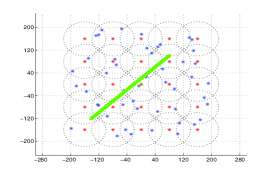
Figure 1: Toplogy (the green line indicates the trajectory of a mobile user).

We assume that all the users request chunks successively from VBR-encoded video sequences. Each video file is a long sequence of chunks, each of duration $0.5$ seconds and with a frame rate of $30$ frames per second. We consider a specific video sequence formed by $800$ chunks, constructed using $4$ video clips from the database in [16], each of length $200$ chunks. The chunks are encoded into different quality modes. Here, the quality index is measured using the Structural SIMilarity (SSIM) index defined in [17]. Figures 2a and 2b show the size in kbits and the SSIM values as a function of the chunk index, respectively, for the different quality modes. The chunks from $1$ to $200$ and $601$ to $800$ are encoded into $8$ quality modes, while the chunks numbered from $201$ to $600$ are encoded in $4$ quality modes. In our experiment, each user starts its streaming session of $1000$ chunks from some arbitrary position in this reference video sequence and successively requests $1000$ chunks by cycling through the sequence. In addition, each user implements a policy to locally estimate the delay with which the video chunks are delivered, such that it can decide its pre-buffering time at the beginning of a streaming session or re-buffering time in the case of a stall event (empty playback buffer) during a streaming session. In addition, it may happen that chunks which go through different queues in the network are affected by different delays. This may give rise to a situation where already received chunks with higher order number cannot be used for playback until the missing chunks with lower order number are also received. In such a case, the policy also provides each user the flexibility to skip a chunk if by doing so, it can provide a large jump in its playback buffer. The complete details of this adaptive playback buffer policy are given in [14]. Figure 3 shows the cumulative distribution function (CDF) of quality (averaged over delivered chunks) over the user population for the values $2V,4V,6V,8V$ and $10V$ with $V=10^{12}$. We can notice the fairness in service as the policy achieves a value close to the optimum for large $V$. We repeat the experiment with the same setup, but now we consider a specific user, indicated by $u_{1}$, moving slowly across the square grid along the green path indicated in Figure 1, during the $1000$ slots of simulation. We fix the parameter $V=10^{13}$ and other parameters of the adaptive playback buffer policy to reasonable values. For the chosen parameters, we observe that the percentage of chunks which are skipped by the mobile user is $1.3\%$ and the pre-buffering time is $162$ time slots. Furthermore, from Figure 4b, showing the evolution of the playback buffer over time, we notice that there are no interruptions and the playback never enters the re-buffering mode. The helpers are numbered from $1$ to $25$, left to right and bottom to top, in Figure 1. In Figure 4a, we plot the helper index providing chunk $k=1,\ldots,1000$ vs. the chunk index. We can observe that as the user moves slowly along the path, the DPP policy “discovers” adaptively the current neighboring helpers and downloads chunks from them in a seamless fashion. Overall, these results are indicative of the dynamic and adaptive nature of the DPP policy in response to arbitrary variations of large-scale pathloss coefficients due to mobility. Extensive simulation results are presented in [14] and are omitted due to space restrictions.

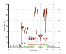
(a) bitrate profile

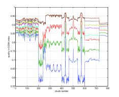
(b) Quality profile

Figure 2: Rate-quality profile of video sequence.

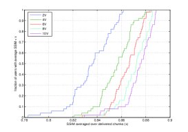
Figure 3: CDF of quality over user population

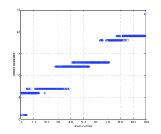
(a) Seamless downloading of chunks.

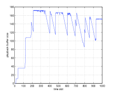
(b) Playback buffer dynamics.

Figure 4: Streaming performance of mobile user

VI Acknowledgement

This material is supported in part by the Intel/Cisco VAWN program and by the Network Science Collaborative Technology Alliance sponsored by the U.S. Army Research Laboratory W911NF-09-2-0053.

References

- [1] M. Neely, “Stochastic network optimization with application to communication and queueing systems,” Synthesis Lectures on Communication Networks, vol. 3, no. 1, pp. 1–211, 2010.
- [2] F. Kelly, “The mathematics of traffic in networks,” The Princeton Companion to Mathematics, 2006.
- [3] Y. Yi and M. Chiang, “Stochastic network utility maximisation-a tribute to Kelly’s paper published in this journal a decade ago,” European Transactions on Telecommunications, vol. 19, no. 4, pp. 421–442, 2008.
- [4] M. Chiang, S. Low, A. Calderbank, and J. Doyle, “Layering as optimization decomposition: A mathematical theory of network architectures,” Proceedings of the IEEE, vol. 95, no. 1, pp. 255–312, 2007.
- [5] M. Neely, E. Modiano, and C. Rohrs, “Dynamic power allocation and routing for time-varying wireless networks,” Selected Areas in Communications, IEEE Journal on, vol. 23, no. 1, pp. 89–103, 2005.
- [6] M. Neely and L. Golubchik, “Utility optimization for dynamic peer-to-peer networks with tit-for-tat constraints,” in INFOCOM, 2011 Proceedings IEEE. IEEE, 2011, pp. 1458–1466.
- [7] D. Bethanabhotla, G. Caire, and M. Neely, “Joint transmission scheduling and congestion control for adaptive streaming in wireless device-to-device networks,” in Proc. Asilomar Conf. on Signals, Systems, and Computers. IEEE, 2012.
- [8] V. Joseph and G. de Veciana, “Jointly optimizing multi-user rate adaptation for video transport over wireless systems: Mean-fairness-variability tradeoffs,” in INFOCOM, 2012 Proceedings IEEE. IEEE, 2012, pp. 567–575.
- [9] Y. Sánchez, T. Schierl, C. Hellge, T. Wiegand, D. Hong, D. De Vleeschauwer, W. Van Leekwijck, and Y. Lelouedec, “iDASH: improved dynamic adaptive streaming over http using scalable video coding,” in ACM Multimedia Systems Conference (MMSys), 2011, pp. 23–25.
- [10] A. Begen, T. Akgul, and M. Baugher, “Watching video over the web: Part 1: Streaming protocols,” Internet Computing, IEEE, vol. 15, no. 2, pp. 54–63, 2011.
- [11] A. Ortega, “Variable bit-rate video coding,” Compressed Video over Networks, pp. 343–382, 2000.
- [12] M. Neely, “Universal scheduling for networks with arbitrary traffic, channels, and mobility,” in Decision and Control (CDC), 2010 49th IEEE Conference on. IEEE, 2010, pp. 1822–1829.
- [13] D. Tse and P. Viswanath, Fundamentals of wireless communication. Cambridge Univ Pr, 2005.
- [14] D. Bethanabhotla, G. Caire, and M. J. Neely, “Joint transmission scheduling and congestion control for adaptive video streaming in small-cell networks,” arXiv preprint arXiv:1304.8083.
- [15] http://www.tsiwireless.com/docs/whitepapers/LTE%20in%20a%20Nutshell%20-%20Physical%20Layer.pdf.
- [16] http://media.xiph.org/video/derf/.
- [17] https://ece.uwaterloo.ca/~z70wang/research/ssim/.