Accurate densities of states for disordered systems from free probability: Live Free or Diagonalize

Abstract

We investigate how free probability allows us to approximate the density of states in tight binding models of disordered electronic systems. Extending our previous studies of the Anderson model in one dimension with nearest-neighbor interactions [J. Chen et al., Phys. Rev. Lett. 109, 036403 (2012)], we find that free probability continues to provide accurate approximations for systems with constant interactions on two- and three-dimensional lattices or with next-nearest-neighbor interactions, with the results being visually indistinguishable from the numerically exact solution. For systems with disordered interactions, we observe a small but visible degradation of the approximation. To explain this behavior of the free approximation, we develop and apply an asymptotic error analysis scheme to show that the approximation is accurate to the eighth moment in the density of states for systems with constant interactions, but is only accurate to sixth order for systems with disordered interactions. The error analysis also allows us to calculate asymptotic corrections to the density of states, allowing for systematically improvable approximations as well as insight into the sources of error without requiring a direct comparison to an exact solution.

I Introduction

Disordered matter is ubiquitous in nature and in manmade materials Ziman (1979). Random media such as glasses Grob (1976); Ford (1982); Debenedetti and Stillinger (2001), disordered alloys Mott and Jones (1958); Tsvelick and Wiegmann (1983), and disordered metals Guttman (1956); Dyre and Schrøder (2000); Dugdale (2005) exhibit unusual properties resulting from the unique physics produced by statistical fluctuations. For example, disordered materials often exhibit unusual electronic properties, such as in the weakly bound electrons in metal–ammonia solutions Kraus (1907); Catterall and Mott (1969); Matsuishi et al. (2003), or in water Walker (1967); Rossky and Schnitker (1988). Paradoxically, disorder can also enhance transport properties of excitons in new photovoltaic systems containing bulk heterojunction layers Peet et al. (2009); McMahon et al. (2011); Yost et al. (2011) and quantum dots Barkai et al. (2004); Stefani et al. (2009), producing anomalous diffusion effects Bouchaud and Georges (1990); Shlesinger et al. (1993); Havlin and Ben-Avraham (2002) which appear to contradict the expected effects of Anderson localization Anderson (1958); Thouless (1974); Belitz and Kirkpatrick (1994). Accounting for the effects of disorder in electro-optic systems is therefore integral for accurately modeling and engineering second–generation photovoltaic devices Difley et al. (2010).

Disordered systems are challenging for conventional quantum methods, which were developed to calculate the electronic structure of systems with perfectly known crystal structures. Determining the electronic properties of a disordered material thus necessitates explicit sampling of relevant structures from thermodynamically accessible regions of the potential energy surface, followed by quantum chemical calculations for each sample. Furthermore, these materials lack long-range order and must therefore be modeled with large supercells to average over possible realizations of short-range order and to minimize finite-size effects. These two factors conspire to amplify the cost of electronic structure calculations on disordered materials enormously.

To avoid such expensive computations, we consider instead calculations where the disorder is treated explicitly in the electronic Hamiltonian. The simplest such Hamiltonian comes from the Anderson model Anderson (1958); Evers and Mirlin (2008), which is a tight binding lattice model of the electronic structure of a disordered electronic medium. Despite its simplicity, this model nonetheless captures the rich physics of strong localization and can be used to model the conductivity of disordered metals Thouless (1974); Belitz and Kirkpatrick (1994). However, the Anderson model cannot be solved exactly except in special cases Halperin (1965); Lloyd (1969), which complicates studies of its excitation and transport properties. Studying more complicated systems thus requires accurate, efficiently computable approximations for the experimental observables of interest.

Random matrix theory offers new possibilities for developing accurate approximate solutions to disordered systems Wigner (1967); Beenakker (2009); Akemann et al. (2011). In this Article, we focus on using random matrix theory to construct efficient approximations for the density of states of a random medium. The density of states is one of the most important quantities that characterize an electronic system, and a large number of physical observables can be calculated from it Kittel (2005). Furthermore, it only depends on the eigenvalues of the Hamiltonian and is thus simpler to approximate, as information about the eigenvectors is not needed. We have previously shown that highly accurate approximations can be constructed using free probability theory for the simplest possible Anderson model, i.e. on a one-dimensional lattice with constant nearest-neighbor interactions Chen et al. (2012). However, it remains to be seen if similar approximations are sufficient to describe more complicated systems, and in particular if the richer physics produced by more complicated lattices and by off-diagonal disorder can be captured using such free probabilistic methods.

In this Article, we present a brief, self–contained introduction to free probability theory in Section II. We then develop approximations from free probability theory in Section III that generalize our earlier study Chen et al. (2012) in three ways. First, we develop analogous approximations for systems with long range interactions, specializing to the simplest such extension of a one-dimensional lattices with next-nearest-neighbor interactions. Second, we study lattices in two and three dimensions. We consider square and hexagonal two-dimensional lattices to investigate the effect of coordination on the approximations. Third, we also make the interactions random and develop approximations for these systems as well. These cases are summarized graphically in Figure 1 and are representative of the diversity of disorder systems described above. Finally, we introduce an asymptotic error analysis which allows us to quantify and analyze the errors in the free probability approximations in Section IV.

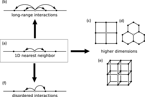
Figure 1: The lattices considered in this work: (a) one-dimensional chain with nearest neighbor interactions, (b) one-dimensional chain with many neighbors, (c) two-dimensional square lattice, (d) two-dimensional hexagonal (honeycomb) lattice, (e) three-dimensional cubic lattice, and (f) one dimensional-chain with disordered interactions.

II Free probability

II.1 Free independence

In this section, we briefly introduce free probability by highlighting its parallels with (classical) probability theory. One of the core ideas in probability theory Feller (1971) is how to characterize the relationship between two (scalar-valued) random variables $x$ and $y$. They may be correlated, so that the joint moment $\left\langle xy\right\rangle$ is not simply the product of the individual expectations $\left\langle x\right\rangle\left\langle y\right\rangle$, or they may be correlated in a higher order moment, i.e. there are some smallest positive integers $m$ and $n$ for which $\left\langle x^{m}y^{n}\right\rangle\neq\left\langle x^{m}\right\rangle\left\langle y^{n}\right\rangle$. If neither case holds, then they are said to be independent, i.e. that all their joint moments of the form $\left\langle x^{m}y^{n}\right\rangle$ factorize into products of the form $\left\langle x^{m}y^{n}\right\rangle=\left\langle x^{m}\right\rangle\left\langle y^{n}\right\rangle$. For random matrices, similar statements can be written down if the expectation $\left\langle\cdot\right\rangle$ is interpreted as the normalized expectation of the trace, i.e. $\left\langle\cdot\right\rangle=\frac{1}{N}\mathbb{E}\mbox{Tr }\cdot$, where $N$ is the size of the matrix. However, matrices in general do not commute, and therefore this notion of independence is no longer unique: for noncommuting random variables, one cannot simply take a joint moment of the form $\left\langle A^{m_{1}}B^{n_{1}}\cdots A^{m_{k}}B^{n_{k}}\right\rangle$ and assert it to be equal in general to $\left\langle A^{m_{1}+\dots+m_{k}}B^{n_{1}+\dots+n_{k}}\right\rangle$. The complications introduced by noncommutativity give rise to a different theory, known as free probability theory, for noncommuting random variables Nica and Speicher (2006). This theory introduces the notion of free independence, which is the noncommutative analogue of (classical) independence. Specifically, two noncommutative random variables $A$ and $B$ are said to be freely independent if for all positive integers $m_{1}$,…,$m_{k}$, $n_{1}$,…,$n_{k}$, the centered joint moment vanishes, i.e.

$$\left\langle\overline{A^{m_{1}}}\ \overline{B^{n_{1}}}\cdots\overline{A^{m_{k}}}\ \overline{B^{n_{k}}}\right\rangle=0,$$ (1)

where we have introduced the centering notation $\overline{A}=A-\left\langle A\right\rangle$. This naturally generalizes the notion of classical independence to noncommuting variables, as the former is equivalent to requiring that all the centered joint moments of the form $\left\langle\overline{x^{m}}\ \overline{y^{n}}\right\rangle$ vanish. If the expectation $\left\langle A\right\rangle$ is reinterpreted as the normalized expectation of the trace of a random matrix $A$, then the machinery of free independence can be applied directly to random matrices Voiculescu (1991).

II.2 Free independence and the $R$-transform

One of the central results of classical probability theory is that if $x$ and $y$ are independent random variables with distributions $p_{X}\left(x\right)$ and $p_{Y}\left(y\right)$ respectively, then the probability distribution of their sum $x+y$ is given by the convolution of the distributions, i.e. Feller (1971)

$$p_{X+Y}\left(y\right)=\int_{-\infty}^{\infty}p_{X}\left(x\right)p_{Y}\left(x-y\right)dx.$$ (2)

An analogous result holds for freely independent noncommuting random variables and is known as the (additive) free convolution; this is most conveniently defined using the $R$-transform Nica and Speicher (2006); Voiculescu (1986); Speicher (2003). For a probability density $p(x)$ supported on $\left[a,b\right]$, its $R$-transform $R\left(w\right)$ is defined implicitly via

$$G(z) =\lim_{\epsilon\rightarrow 0^{+}}\int_{a}^{b}\frac{p(x)}{z-\left(x+i\epsilon\right)}dx$$ (3a)

$$R(w) =G^{-1}(w)-\frac{1}{w}.$$ (3b)

These quantities have natural analogues in Green function theory: $p\left(x\right)$ is the density of states, i.e. the distribution of eigenvalues of the underlying random matrix; $G$$\left(z\right)$ is the Cauchy transform of $p\left(x\right)$, which is the retarded Green function; and $G^{-1}\left(w\right)=R\left(w\right)+1/w$ is the self-energy. The $R$-transform allows us to define the free convolution of $A$ and $B$, denoted $A\boxplus$B, by adding the individual $R$-transforms

$$R_{A\boxplus B}\left(w\right):=R_{A}\left(w\right)+R_{B}\left(w\right).$$ (4)

This finally allows to state that if $A$ and $B$ are freely independent, then the sum $A+B$ must satisfy

$$R_{A+B}\left(w\right)=R_{A\boxplus B}\left(w\right).$$ (5)

In general, random matrices $A$ and $B$ are neither classically independent nor freely independent. However, we can always construct combinations of them that are always freely independent. One such combination is $A+Q^{\dagger}BQ$, where $Q$ is a random orthogonal (unitary) matrix of uniform Haar measure, as applied to real symmetric (Hermitian) $A$ and $B$ Edelman and Rao (2005). The similarity transform effected by $Q$ randomly rotates the basis of $B$, so that the eigenvectors of $A$ and $B$ are always in generic position, i.e. that any eigenvector of $A$ is uncorrelated with any eigenvector of $B$ Akemann et al. (2011). This is the main result that we wish to exploit. While in general $A$ and $B$ are not freely independent, and hence (5) fails to hold exactly, we can nonetheless make the approximation that (5) holds approximately, and use this as a way to calculate the density of states of a random matrix $H$ using only its decomposition into a matrix sum $H=A+B$. Our application of this idea to the Anderson model is described below.

III Numerical results

III.1 Computation of the Density of States and its Free Approximant

We now wish to apply the framework of free probability theory to study Anderson models beyond the one-dimensional nearest-neighbor model which was the focus of our initial study Chen et al. (2012). It is well-known that more complicated Anderson models exhibit rich physics that are absent in the simplest case. First, the one-dimensional Anderson Hamiltonian with long range interactions has delocalized eigenstates at low energies and an asymmetric density of states, features that are absent in the simplest Anderson model Cressoni and Lyra (1998); de Brito et al. (2004); de Moura et al. (2005); Malyshev et al. (2004); Rodríguez et al. (2003). These long range interactions give rise to slowly decaying interactions in many systems, such as spin glasses Ford (1982); Binder and Young (1986) and ionic liquids Pitzer et al. (1985). Second, two-dimensional lattices can exhibit weak localization Abrahams et al. (1979), which is responsible for the unusual conductivities of low temperature metal thin films Dolan and Osheroff (1979); Bergmann (1984). The hexagonal (honeycomb) lattice is of particular interest as a tight binding model for nanostructured carbon allotropes such as carbon nanotubes Saito et al. (1999) and graphene Hobson and Nierenberg (1953); Castro Neto et al. (2009), which exhibit novel electronic phases with chirally tunable band gaps Hamada et al. (1992); Samarakoon and Wang (2010) and topological insulation Castro Neto et al. (2006); Moore (2010). Third, the Anderson model in three dimensions exhibits nontrivial localization phases that are connected by the metal–insulator transition Anderson (1958); Schönhammer and Brenig (1973). Fourth, systems with off-diagonal disorder, such as substitutional alloys and Frenkel excitons in molecular aggregates Ziman (1979); Fidder et al. (1991), exhibit rich physics such as localization transitions in lattices of any dimension Antoniou and Economou (1977), localization dependence on lattice geometry Hu et al. (1984), Van Hove singularities Brezini (1990), and asymmetries in the density of states Fidder et al. (1991). Despite intense interest in the effects of off-diagonal disorder, such systems have resisted accurate modeling Blackman et al. (1971); Koepernik et al. (1998); Esterling (1975); Elliott et al. (1974); Tanaka et al. (1971); Bishop and Mookerjee (1974); Shiba (1971); Schwartz and Siggia (1972); Schwartz et al. (1973). We are therefore interested to find out if our approximations as developed in our initial study Chen et al. (2012) can be applied also to all these disordered systems.

The Anderson model can be represented in the site basis by the matrix with elements

$$H_{ij}=g_{i}\delta_{ij}+J_{ij}$$ (6)

where $g_{i}$ is the energy of site $i$, $\delta_{ij}$ is the usual Kronecker delta, and $J_{ij}$ is the matrix of interactions with $J_{ii}=0$. Unless otherwise specified, we further specialize to the case of constant interactions between connected neighbors, so that $J_{ij}=JM_{ij}$ where $J$ is a scalar constant representing the interaction strength, and $M$ is the adjacency matrix of the underlying lattice. Unless specified otherwise, we also apply vanishing (Dirichlet) boundary conditions, as this reduces finite-size fluctuations in the density of states relative to periodic boundary conditions. For concrete numerical calculations, we also choose the site energies $g_{i}$ to be iid Gaussian random variables of variance $\sigma^{2}$ and mean 0. With these assumptions, the strength of disorder in the system can be quantified by a single dimensionless parameter $\sigma/J$.

The particular quantity we are interested in approximating is the density of states, which is one of the most important descriptors of electronic band structure in condensed matter systems Kittel (2005). It is defined as the distribution

$$\rho_{H}\left(x\right)=\left\langle\sum_{j}\delta\left(x-\epsilon_{j}\right)\right\rangle$$ (7)

where $\epsilon_{j}$ is the $j$th eigenvalue of a sample of $H$ and the expectation $\left\langle\cdot\right\rangle$ is the ensemble average.

To apply the approximations from free probability theory, we partition our Hamiltonian matrix into its diagonal and off–diagonal components $A$ and $B$. The density of states of $A$ is simply a Gaussian of mean 0 and variance $\sigma^{2}$, and for many of our cases studied below, the density of states of $B$ is proportional to the adjacency matrix of well–known graphs Strang (1999) and hence is known analytically. We then construct the free approximant

$$H^{\prime}=A+Q^{T}BQ$$ (8)

where $Q$ is a random orthogonal matrix of uniform Haar measure as discussed in Section II.2, and find its density of states $\rho_{H^{\prime}}$. Specific samples of $Q$ can be generated by taking the orthogonal part of the QR decomposition Golub and van Loan (1996) of matrix from the Gaussian orthogonal ensemble (GOE) Diaconis (2005). We then average the approximate density of states over many realizations of the Hamiltonian and $Q$ and compare it to the ensemble averaged density of states generated from exact diagonalization of the Hamiltonian. We choose the number of samples to be sufficient to converge the density of states with respect to the disorder in the Hamiltonian. While this is not the most efficient way of computing free convolutions, it provides a general and robust test for the quality of the free approximation. The free approximant can be computed efficiently using numerical free convolution techniques Olver and Nadakuditi .

III.2 One-dimensional chain

We now proceed to apply the theory of the previous section to specific examples of the Anderson model on various lattices. Previously, we had studied the Anderson model on the one-dimensional chain Chen et al. (2012):

$$H_{ij}=g_{i}\delta_{ij}+J\left(\delta_{i,j+1}+\delta_{i,j-1}\right),$$ (9)

which is arguably the simplest model of a disordered system. Despite its simple tridiagonal form, this Hamiltonian does not have an exact solution for its density of states, and many approximations for it have been developed Yonezawa and Morigaki (1973). However, unlike the original Hamiltonian, the diagonal and off-diagonal components each have a known density of states when considered separately. To calculate the density of states of the Hamiltonian, we diagonalized 1000 samples of $1000\times 1000$ matrices, so that the resulting density of states is converged with respect to both disorder and finite-size effects. The results are shown in Figure 2(a), demonstrating that the free approximation to the density of states is visually indistinguishable from the exact result over all the entire possible range of disorder strength $\sigma/J$.

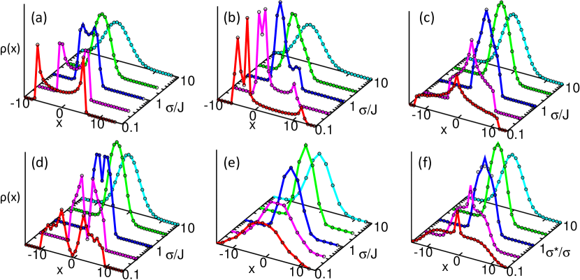
Figure 2: Comparison of exact density of states (lines) with free probability approximant (circles) for the lattices in Figure 1, with (b) showing the case of $n=4$ neighbors. Data are shown for multiple values of a dimensionless parameter quantifying the strength of disorder to show the robustness of this approximation. For (a-e), this parameter is $\sigma/J$, the ratio of the noisiness of diagonal elements to the strength of off-diagonal interaction. In (f), the axis is chosen to be the relative strength of off-diagonal disorder to diagonal disorder, $\sigma^{*}/\sigma$, with $\sigma/J=1$.

III.3 One-dimensional lattice with non-neighbor interactions

Going beyond tridiagonal Hamiltonians, we next study the Anderson model on a one-dimensional chain with constant interactions to $n$ neighbors. The Hamiltonian then takes the form:

$$H_{ij}^{1D}=g_{i}\delta_{ij}+J\left[\sum_{k=1}^{n}\delta_{i,j+k}+\delta_{i+k,j}\right].$$ (10)

where we use the superscript to distinguish the one-dimensional many-neighbor Hamiltonian from its higher dimensional analogs. Unlike the nearest-neighbor interaction case above, the density of states is known to exhibit Van Hove singularities at all but the strongest disorder Thouless (1974); Ziman (1979).

We average over 1000 samples of $1000\times 1000$ Hamiltonians, which as before ensures that the density of states is numerically converged with respect to statistical fluctuations and finite-size effects. We looked at the case of $n=2,...,6$ neighbors with identical interaction strengths, and also interaction strengths that decayed linearly with distance to better model the decay of interactions with distance in more realistic systems. The free approximant is of similar quality in all cases. As shown in Figure 2(b) for $n=4$ neighbors, the free approximant reproduces these singular features of the density of states, unlike perturbative methods which are known to smooth them out Allan (1984); Haydock (1980). The reproduction of singularities by the free approximant parallels similar observations found in other applications of free probability to quantum information theory Movassagh and Edelman (2011).

III.4 Square, hexagonal and cubic lattices

We now investigate the effect of dimensionality on the accuracy of the free approximant in three lattices. First, we consider the Anderson model on the square lattice, with Hamiltonian:

$$H^{2D}=B^{1D}\otimes I+I\otimes B^{1D}+A$$ (11)

where $B^{1D}$ is the off-diagonal part of the $H^{1D}$ defined in equation (10), $I$ is the identity matrix with the same dimensions as $B^{1D}$, $A$ is the diagonal matrix of independent random site energies of appropriate dimension, and $\otimes$ is the Kronecker (direct) product. We have found that a square lattice of $50\times 50=2500$ sites is the smallest lattice with negligible finite size fluctuations in the density of states. As such, we calculated the density of states for 500 samples of $3600\times 3600$ Hamiltonians. We find that for both nearest-neighbors (shown in Figure 2(c)) and non-nearest-neighbors (specifically, $n=2,...,6$), the free approximation is again visually identical to the exact answer.

Second, we consider the honeycomb (hexagonal) lattice, which has a lower coordination number than the square lattice. Its adjacency matrix does not have a simple closed form, but can nonetheless be easily generated. For this lattice, we averaged over 1000 samples of matrices of size $968\times 968$, and applied periodic boundary conditions to illustrate their effect. As in the square case of the two dimensional grid model, the density of states of the honeycomb lattice with any number of coupled neighbor shells is well reproduced by the free approximant (Figure 2(d)), even reproducing the Van Hove singularities at low to moderate site disorder. Additionally, we see that the finite-size oscillations at low disorder ($\sigma/J\sim 0.1$) are also reproduced by the free approximation.

Third, we consider the Anderson model on a cubic lattice, whose Hamiltonian is:

$$H^{3D}=\left(B^{1D}\otimes I\otimes I\right)+\left(I\otimes B^{1D}\otimes I\right)+\left(I\otimes I\otimes B^{1D}\right)+A$$ (12)

Figure 2(e) shows the approximate and exact density of states calculated from 1000 samples of $1000\times 1000$ matrices. This represents a $10\times 10\times 10$ cubic lattice which is significantly smaller in linear dimension than the previously considered lattices. We therefore observed oscillatory features in the density of states arising from finite-size effects. Despite this, the free approximant is still able to reproduce the exact density of states quantitatively. In fact, if the histogram in Figure 2(e) is recomputed with finer histogram bins to emphasize the finite-size induced oscillations, we still observe that the free approximant reproduces these features.

III.5 Off-diagonal disorder

Up to this point, all of the models we have considered have only site disorder, with no off-diagonal disorder. Free probability has thus far provided a qualitatively correct approximation for all these lattices. To test the robustness of this approximation, we now investigate systems with random interactions. The simplest such system is the one-dimensional chain, with a Hamiltonian of the form:

$$H_{ij}=g_{i}\delta_{ij}+h_{i}\left(\delta_{i,j+1}+\delta_{i,j-1}\right).$$ (13)

Unlike in the previous systems, the interactions are no longer constant, but are instead new random variables $h_{i}$. We choose them to be Gaussians of mean $J$ and variance $\left(\sigma^{*}\right)^{2}$. There are now two order parameters to consider: $\sigma^{*}/J$, the relative disorder in the interaction strengths, and $\sigma^{*}/\sigma$, the strength of off-diagonal disorder relative to site disorder. As in the prior one-dimensional case, we average over 1000 realizations of $1000\times 1000$ matrices.

We now observe that the quality of the free approximation is no longer uniform across all values of the order parameters. Instead, it varies with $\sigma^{*}/\sigma$, but not $\sigma^{*}/J$. In Figure 2(f), we demonstrate the results of varying $\sigma^{*}/\sigma$ with $\sigma/J=1$. In the limits $\sigma^{*}/\sigma\gg 1$ and $\sigma^{*}/\sigma\ll 1$, the free approximation matches the exact result well; however, there is a small but noticeable discrepancy between the exact and approximate density of states for moderate relative off-diagonal disorder, though the quality of the approximation is mostly unaffected by the centering of the off-diagonal disorder. In the next section, we will investigate the nontrivial behavior of the approximation with the $\sigma^{*}/\sigma$ order parameter.

IV Error analysis

In our numerical experiments, we have found that the accuracy of the free approximation remains excellent for systems with only site disorder, regardless of the underlying lattice topology or the number of interactions that each site has. Details such as finite-size oscillations and Van Hove singularities are also captured when present. However, when off-diagonal disorder is present, the quality of the approximation does vary qualitatively with the ratio of off-diagonal disorder to site disorder $\sigma^{*}/\sigma$ as illustrated in Section III.5, and the error is greatest when $\sigma^{*}\approx\sigma$. To understand the reliability of the free approximant (8) in all these situations, we apply an asymptotic moment expansion to calculate the leading order error terms for the various systems. In general, a probability density $\rho$ can be expanded with respect to another probability density $\tilde{\rho}$ in an asymptotic moment expansion known as the Edgeworth series Chen and Edelman ; Stuart and Ord (1994):

$$\rho\left(x\right)=\exp\left(\sum_{m=1}^{\infty}\frac{\kappa^{\left(m\right)}-\tilde{\kappa}^{\left(m\right)}}{m!}\left(-\frac{d}{dx}\right)^{m}\right)\tilde{\rho}\left(x\right)$$ (14)

where $\kappa^{\left(m\right)}$ is the $m$th cumulant of $\rho$ and $\tilde{\kappa}^{\left(m\right)}$ is the $m$th cumulant of $\tilde{\rho}$. When all the cumulants exist and are finite, this is an exact relation that allows for the distribution $\tilde{\rho}$ to be systematically corrected to become $\rho$ by substituting in the correct cumulants. If the first $\left(n-1\right)$ cumulants of $\rho$ and $\tilde{\rho}$ match, but not the $n$th, then we can calculate the leading-order asymptotic correction to $\tilde{\rho}$ as:

$$\rho(x) =\exp\left(\frac{\kappa^{\left(n\right)}-\tilde{\kappa}^{\left(n\right)}}{n!}\left(-\frac{d}{dx}\right)^{n}+\dots\right)\tilde{\rho}(x)$$ (15a)

$$=\left(1+\frac{\kappa^{\left(n\right)}-\tilde{\kappa}^{\left(n\right)}}{n!}\left(-\frac{d}{dx}\right)^{n}+\dots\right)\tilde{\rho}(x)$$ (15b)

$$=\tilde{\rho}\left(x\right)+\frac{(-1)^{n}}{n!}\left(\kappa^{\left(n\right)}-\tilde{\kappa}^{\left(n\right)}\right)\frac{d^{n}\tilde{\rho}}{dx^{n}}(x)+\mathcal{O}\left(\frac{d^{n+1}\tilde{\rho}}{dx^{n+1}}\right)$$ (15c)

$$=\tilde{\rho}\left(x\right)+\frac{(-1)^{n}}{n!}\left(\mu^{\left(n\right)}-\tilde{\mu}^{\left(n\right)}\right)\frac{d^{n}\tilde{\rho}}{dx^{n}}(x)+\mathcal{O}\left(\frac{d^{n+1}\tilde{\rho}}{dx^{n+1}}\right)$$ (15d)

where on the second line we expanded the exponential $e^{X}=1+X+\dots$, and on the fourth line we used the well-known relationship between cumulants $\kappa$ and moments $\mu$ and the fact that the first $n-1$ moments of $\rho$ and $\tilde{\rho}$ were identical by assumption.

We can now use this expansion to calculate the leading-order difference between the exact density of states $\rho_{H}=\rho_{A+B}$, and its free approximant $\rho_{H^{\prime}}=\rho_{A\boxplus B}$ by setting $\tilde{\rho}=\rho_{H^{\prime}}$ and $\rho=\rho_{H}$ in (15d). The only additional data required are the moments $\mu_{H}^{\left(n\right)}=\left\langle H^{n}\right\rangle$ and $\mu_{H^{\prime}}^{\left(n\right)}=\left\langle\left(H^{\prime}\right)^{n}\right\rangle$, which can be computed from the sampled data or recursively from the joint moments of $A$ and $B$ as detailed elsewhere Chen and Edelman . This then gives us a way to detect discrepancies, which is to calculate successively higher moments of $H$ and $H^{\prime}$ to determine whether the difference in moments is statistically significant, and then for the smallest order moment that differs, calculate the correction using (15d).

The error analysis also yields detailed information about the source of error in the free approximation. The $n$th moment of $H$ is given by

$$\mu_{H}^{(n)}=\left\langle H^{n}\right\rangle=\left\langle\left(A+B\right)^{n}\right\rangle=\sum_{\begin{array}[]{c}{\scriptstyle m_{1},n_{1},\dots,m_{k},n_{k}}\\ {\scriptstyle\sum_{j=1}^{k}m_{j}+n_{j}=n}\end{array}}\left\langle A^{m_{1}}B^{n_{1}}\cdots A^{m_{k}}B^{n_{k}}\right\rangle,$$ (16)

where the last equality arises from expanding $\left(A+B\right)^{n}$ in a noncommutative binomial series. If $A$ and $B$ are freely independent, then each of these terms must satisfy recurrence relations that can be derived from the definition (1) Chen and Edelman . Exhaustively enumerating and examining each of the terms in the final sum to see if they satisfy (1) thus provides detailed information about the accuracy of the free approximation.

We now apply this general error analysis for the specific systems we have studied. It turns out that the results for systems with and without off-diagonal disorder exhibit different errors, and so are presented separately below.

IV.1 Systems with constant interactions

We have previously shown that for the one-dimensional chain with nearest-neighbor interactions, the free approximant is exact in the first seven moments, and that the only term in the eighth moment that differs between the free approximant and the exact $H$ is $\left\langle\left(AB\right)^{4}\right\rangle$ Chen et al. (2012). The value of this joint moment can be understood in terms of discretized hopping paths on the lattice Wigner (1967). Writing out the term $\left\langle\left(AB\right)^{4}\right\rangle$ explicitly in terms of matrix elements and with Einstein’s implicit summation convention gives:

$$\left\langle\left(AB\right)^{4}\right\rangle =\frac{1}{N}\mathbb{E}\left(A_{i_{1}i_{2}}B_{i_{2}i_{3}}A_{i_{3}i_{4}}B_{i_{4}i_{5}}A_{i_{5}i_{6}}B_{i_{6}i_{7}}A_{i_{7}i_{8}}B_{i_{8}i_{1}}\right)$$ (17a)

$$=\frac{1}{N}\mathbb{E}\left(\left(g_{i_{1}}\delta_{i_{1}i_{2}}\right)\left(JM_{i_{2}i_{3}}\right)\left(g_{i_{3}}\delta_{i_{3}i_{4}}\right)\left(JM_{i_{4}i_{5}}\right)\left(g_{i_{5}}\delta_{i_{5}i_{6}}\right)\left(JM_{i_{6}i_{7}}\right)\left(g_{i_{7}}\delta_{i_{7}i_{8}}\right)\left(JM_{i_{8}i_{1}}\right)\right)$$ (17b)

$$=\frac{1}{N}\mathbb{E}\left(g_{i_{1}}g_{i_{2}}g_{i_{3}}g_{i_{4}}J^{4}M_{i_{1}i_{2}}M_{i_{2}i_{3}}M_{i_{3}i_{4}}M_{i_{4}i_{1}}\right).$$ (17c)

From this calculation, we can see that each multiplication by $A$ weights each path by the site energy of a given site, $g_{i}$, and each multiplication by $B$ weights the path by $J$ and causes the path to hop to a coupled site. The sum therefore reduces to a weighted sum over returning paths on the lattice that must traverse exactly three intermediate sites. The only paths on the lattice with nearest-neighbors that satisfy these constraints are shown in Figure 3(a), namely $\left(i_{1},i_{2},i_{3},i_{4}\right)=\left(k,k+1,k,k+1\right)$, $\left(k,k+1,k+2,k+1\right)$, $\left(k,k-1,k,k-1\right)$, and $\left(k,k-1,k-2,k-1\right)$ for some starting site $k$. The first path contributes weight $\mathbb{E}\left(g_{k}^{2}g_{k+1}^{2}\right)J^{4}=\mathbb{E}\left(g_{k}^{2}\right)\mathbb{E}\left(g_{k+1}^{2}\right)J^{4}=\sigma^{4}J^{4}$ while the second term has weight $\mathbb{E}\left(g_{k}g_{k+1}^{2}g_{k+2}\right)J^{4}=\mathbb{E}\left(g_{k}\right)\mathbb{E}\left(g_{k+1}^{2}\right)\mathbb{E}\left(g_{k+2}\right)J^{4}=0$. Similarly, the third and fourth paths also have weight $\sigma^{4}J^{4}$ and 0 respectively. Finally averaging over all possible starting sites, we arrive at the final result that $\left\langle\left(AB\right)^{4}\right\rangle=2\sigma^{4}J^{4}$ with periodic boundary conditions and $\left\langle\left(AB\right)^{4}\right\rangle=2\left(1-1/N\right)\sigma^{4}J^{4}$ with vanishing boundary conditions. We therefore see when $N$ is sufficiently large, the boundary conditions contribute a term of $\mathcal{O}\left(1/N\right)$ which can be discarded, thus showing the universality of this result regardless of the boundary conditions.

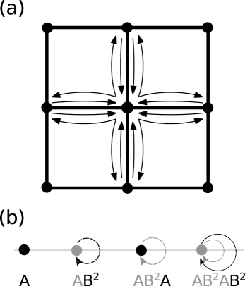
Figure 3: (a) Diagrammatic representation of the four paths that contribute to the leading order error for the case of a two-dimensional square lattice with constant interactions and nearest neighbors. Dots contribute a factor of $g_{i}$ for site $i$. Solid arrows represent a factor of $J$. Each path contributes $J^{4}\left\langle g_{a}^{2}\right\rangle\left\langle g_{b}^{2}\right\rangle=\sigma^{4}J^{4}$ to the error. (b) Build up of the diagrammatic representation the leading order error in the case of a 1D chain with off-diagonal disorder. The two dashed arrows contribute a factor of $\mu_{4}-\mu_{2}^{2}$. Because of the disorder in the interactions, multiplication by $\overline{B^{2}}$ allows loops back to the same site. The first of these loops, $\left\langle\overline{A}\overline{B^{2}}\right\rangle$, has zero expectation value because it contains an independent random variable of mean zero as a factor. Once two loops are present, the expectation value instead contains this random variable squared, which has nonzero expectation value.

Applying the preceding error analysis, we observe that the result from the one-dimensional chain generalizes all the other systems with constant interactions that we have studied; the only difference being that the coefficient 2 is simply replaced by $n$, the number of sites accessible in a single hop from a given lattice site. In order to keep the effective interaction felt by a site constant as we scale $n$, we can choose $J$ to scale as $\frac{1}{\sqrt{n}}$. In this case, the free approximation converges to the exact result as $\frac{1}{n}$.

We can generalize the argument presented above to explain why $\left\langle\left(\overline{A}\overline{B}\right)^{4}\right\rangle$ is the first nonzero joint centered moment, and thus why the approximation does not break down before the eighth moment. Consider centered joint moments of the form:

$$\left\langle\overline{A^{a_{1}}}\overline{B^{b_{1}}}\overline{A^{a_{2}}}\overline{B^{b_{2}}}\ldots\overline{A^{a_{n}}}\overline{B^{b_{n}}}\right\rangle$$ (18)

for positive integers $\{a_{i},b_{i}\}$ such that $\sum_{i}(a_{i}+b_{i})\leq 8$. Since $A$ is diagonal with iid elements, all powers of $A^{n}$ are also diagonal with iid elements, and so $\overline{A^{n}}=0$. Centered higher powers of $B$, $\overline{B^{n}}$, couple each site to other sites with interaction strengths $J^{n}$, but after centering, the diagonal elements of $\overline{B^{n}}$ are zero and multiplication by $\overline{B^{n}}$ still represents a hop from one site to a different coupled site. Therefore, the lowest order nonzero joint centered moment requires at least four hops, so $n\geq 4$ is the smallest possible nonzero term, but but the only term of this form of eighth order or lower is the one with $a_{i}=b_{i}=1$, i.e. the term $\left\langle\left(AB\right)^{4}\right\rangle$.

IV.2 Random interactions

When the off-diagonal interactions are allowed to fluctuate, the free approximation breaks down in the sixth moment, where the joint centered moment $\left\langle\left(\overline{A}\overline{B^{2}}\right)^{2}\right\rangle$ fails to vanish. We can understand this using a generalization of the hopping explanation from before. In this case, $\overline{B^{2}}$ contains nonzero diagonal elements, which corresponds to a nonzero weight for paths that stay at the same site. Thus, $\left(\overline{A}\overline{B^{2}}\right)^{2}$ contains a path of nonzero weight that starts at a site and loops back to that site twice (shown in Figure 3(b)). The overall difference in the moment of the exact distribution from that in the free distribution is $2\sigma^{2}\left(\mu_{4}-\mu_{2}^{2}\right)$, where $\mu_{4}$ and $\mu_{2}$ are the fourth and second moments of the off-diagonal disorder. As above, the $\sigma^{2}$ component of this difference can be understood as the contribution of the two $A$s in the joint centered moment. The other factor, $2\left(\mu_{4}-\mu_{2}^{2}\right)$, is the weight of the path of two consecutive self-loops. The sixth moment is the first to break down because, as before, we must hop to each node on our path twice in order to avoid multiplying by the expectation value of mean zero, and $\left(AB^{2}\right)^{2}$ is the lowest order term that allows such a path.

We summarize the the leading order corrections and errors in Table 1. At this point, we introduce the quantity $\tilde{J}=\sqrt{2n}J$, which is an aggregate measure of the interactions of any site with all its $2n$ neighbors. As can be seen, the discrepancy occurs to eighth order for all the studied systems with constant interactions, with a numerical prefactor indicative of the coordination number of the lattice, and the factor of 1/8! strongly suppresses the contribution of the error terms. Furthermore, for any given value of the total interaction $\tilde{J}$, the error decreases quickly with coordination number $2n$, suggesting that the free probability approximation is exact in the mean field limit of $2n\rightarrow\infty$ neighbors. This is consistent with previous studies of the Anderson model employing the coherent potential approximation.Thouless (1974); Neu and Speicher (1995a, b) In contrast, the system with off-diagonal disorder has a discrepancy in the sixth moment, which has a larger coefficient in the Edgeworth expansion (15d). This explains the correspondingly poorer performance of our free approximation for systems with off-diagonal disorder. Furthermore, the preceding analysis shows that only the first and second moments of the diagonal disorder $\sigma$ contribute to the correction coefficient, thus showing that this behavior is universal for disorder with finite mean and standard deviation.

Table 1: Coefficients of the leading-order error in the free probability approximation in the Edgeworth expansion (15d).

	Order	Term	Coefficient
1D	8	$\left(AB\right)^{4}$	$\tilde{J}^{4}\sigma^{4}/\left(2\cdot 8!\right)$
2D square	8	$\left(AB\right)^{4}$	$\tilde{J}^{4}\sigma^{4}/\left(4\cdot 8!\right)$
2D honeycomb	8	$\left(AB\right)^{4}$	$\tilde{J}^{4}\sigma^{4}/\left(3\cdot 8!\right)$
3D cube	8	$\left(AB\right)^{4}$	$\tilde{J}^{4}\sigma^{4}/\left(6\cdot 8!\right)$
1D with $n$ nearest-neighbors	8	$\left(AB\right)^{4}$	$\tilde{J}^{4}\sigma^{4}/\left(2n\cdot 8!\right)$
1D with off-diagonal disorder	6	$\left(AB^{2}\right)^{2}$	$\sigma^{2}\left(\mu_{4}-\mu_{2}^{2}\right)/6!$

V Conclusion

Free probability provides accurate approximations to the density of states of a disordered system, which can be constructed by partitioning the Hamiltonian into two easily-diagonalizable ensembles and then free convolving their densities of states. Previous work Chen et al. (2012) showed that this approximation worked well for the one-dimensional Anderson model partitioned into its diagonal and off-diagonal components. Our numerical and theoretical study described above demonstrates that the same approximation scheme is widely applicable to a diverse range of systems, encompassing more complex lattices and more interactions beyond the nearest-neighbor. The quality of the approximation remains unchanged regardless of the lattice as long as the interactions are constant, with the free approximation being in error only in the eighth moment of the density of states. When the interactions fluctuate, the quality of the approximation worsens, but remains exact in the first five moments of the density of states.

Our results strongly suggest that free probability has the potential to produce high-quality approximations for the properties of disordered systems. In particular, our theoretical analysis of the errors reveals universal features of the quality of the approximation, with the error being characterized entirely by the moments of the relevant fluctuations and the local topology of the lattice. This gives us confidence that approximations constructed using free probability will give us high-quality results with rigorous error quantification. This also paves the way for future investigations for constructing fast free convolutions using numerical methods for $R$-transforms,Olver and Nadakuditi which would yield much faster methods for constructing free approximations. Additionally, further studies will be required to approximate other observables of interest such as conductivities and phase transition points. These will require further theoretical investigation into how free probability can help predict properties of eigenvectors, which may involve generalizing some promising initial studies linking the statistics of eigenvectors such as their inverse participation ratios to eigenvalue statistics such as the spectral compressibility Klesse and Metzler (1997); Bogomolny and Giraud (2011).

References

- Ziman (1979) J. M. Ziman, Models of Disorder: The Theoretical Physics of Homogeneously Disordered Systems (Cambridge University Press, Oxford, 1979).
- Grob (1976) D. Grob, ed., The Glass Transition and the Nature of the Glassy State (New York Academy of Sciences, New York, 1976).
- Ford (1982) P. J. Ford, Contemp. Phys. 23, 141 (1982).
- Debenedetti and Stillinger (2001) P. G. Debenedetti and F. H. Stillinger, Nature 410, 259 (2001).
- Mott and Jones (1958) N. Mott and H. Jones, The Theory of the Properties of Metals and Alloys (Dover Publications, New York, 1958).
- Tsvelick and Wiegmann (1983) A. Tsvelick and P. Wiegmann, Adv. Phys. 32, 453 (1983).
- Guttman (1956) L. Guttman, Solid State Phys. 3, 145 (1956).
- Dyre and Schrøder (2000) J. Dyre and T. Schrøder, Rev. Mod. Phys. 72, 873 (2000).
- Dugdale (2005) J. S. Dugdale, The Electrical Properties of Disordered Metals, Cambridge Solid State Science Series (Cambridge, Cambridge, UK, 2005).
- Kraus (1907) C. Kraus, J. Am. Chem. Soc. 29, 1557 (1907).
- Catterall and Mott (1969) R. Catterall and N. Mott, Adv. Phys. 18, 665 (1969).
- Matsuishi et al. (2003) S. Matsuishi, Y. Toda, M. Miyakawa, K. Hayashi, T. Kamiya, M. Hirano, I. Tanaka, and H. Hosono, Science 301, 626 (2003).
- Walker (1967) D. C. Walker, Q. Rev. Chem. Soc. 21, 79 (1967).
- Rossky and Schnitker (1988) P. J. Rossky and J. Schnitker, J. Phys. Chem. 92, 4277 (1988).
- Peet et al. (2009) J. Peet, A. J. Heeger, and G. C. Bazan, Acc. Chem. Res. 42, 1700 (2009).
- McMahon et al. (2011) D. P. McMahon, D. L. Cheung, and A. Troisi, J. Phys. Chem. Lett. 2, 2737 (2011).
- Yost et al. (2011) S. R. Yost, L.-P. Wang, and T. Van Voorhis, J. Phys. Chem. C 115, 14431 (2011).
- Barkai et al. (2004) E. Barkai, Y. Jung, and R. Silbey, Annu. Rev. Phys. Chem. 55, 457 (2004).
- Stefani et al. (2009) F. D. Stefani, J. P. Hoogenboom, and E. Barkai, Phys. Today 62, 34 (2009).
- Bouchaud and Georges (1990) J.-P. Bouchaud and A. Georges, Phys. Rep. 195, 127 (1990).
- Shlesinger et al. (1993) M. F. Shlesinger, G. M. Zaslavsky, and J. Klafter, Nature 363, 31 (1993).
- Havlin and Ben-Avraham (2002) S. Havlin and D. Ben-Avraham, Adv. Phys. 51, 187 (2002).
- Anderson (1958) P. W. Anderson, Phys. Rev. 109, 1492 (1958).
- Thouless (1974) D. J. Thouless, Phys. Rep. 13, 93 (1974).
- Belitz and Kirkpatrick (1994) D. Belitz and T. R. Kirkpatrick, Rev. Mod. Phys. 66 (1994).
- Difley et al. (2010) S. Difley, L.-P. Wang, S. Yeganeh, S. R. Yost, and T. Van Voorhis, Acc. Chem. Res. 43, 995 (2010).
- Evers and Mirlin (2008) F. Evers and A. Mirlin, Rev. Mod. Phys. 80, 1355 (2008).
- Halperin (1965) B. Halperin, Phys. Rev. 139, A104 (1965).
- Lloyd (1969) P. Lloyd, J. Phys. C: Solid State Phys. 2, 1717 (1969).
- Wigner (1967) E. P. Wigner, SIAM Rev. 9, 1 (1967).
- Beenakker (2009) C. W. J. Beenakker, arXiv:0904.1432 (2009), arXiv:0904.1432 .
- Akemann et al. (2011) G. Akemann, J. Baik, and P. Di Francesco, eds., The Oxford Handbook of Random Matrix Theory (Oxford University Press, Oxford; New York, 2011).
- Kittel (2005) C. Kittel, Introduction to Solid State Physics, 8th ed. (Wiley, Hoboken, NJ, 2005).
- Chen et al. (2012) J. Chen, E. Hontz, J. Moix, M. Welborn, T. Van Voorhis, A. Suárez, R. Movassagh, and A. Edelman, Phys. Rev. Lett. 109, 036403 (2012).
- Feller (1971) W. Feller, An Introduction to Probability Theory and Its Applications, Vol. 2, 2nd ed. (John Wiley, New York, 1971).
- Nica and Speicher (2006) A. Nica and R. Speicher, Lectures on the combinatorics of free probability (Cambridge University Press, Cambridge, 2006).
- Voiculescu (1991) D. Voiculescu, Invent. Math. 104, 201 (1991).
- Voiculescu (1986) D. Voiculescu, J. Funct. Anal. 66, 323 (1986).
- Speicher (2003) R. Speicher, in Asymptotic Combinatorics with Application to Mathematical Physics, July, edited by A. M. Vershik (St. Petersburg, 2003) pp. 53–73.
- Edelman and Rao (2005) A. Edelman and N. R. Rao, Acta Numerica 14, 233 (2005).
- Cressoni and Lyra (1998) J. C. Cressoni and M. L. Lyra, Physica A 256, 18 (1998).
- de Brito et al. (2004) P. de Brito, E. Rodrigues, and H. Nazareno, Phys. Rev. B 69, 214204 (2004).
- de Moura et al. (2005) F. de Moura, A. Malyshev, M. Lyra, V. Malyshev, and F. Domínguez-Adame, Phys. Rev. B 71, 174203 (2005).
- Malyshev et al. (2004) A. Malyshev, V. Malyshev, and F. Domínguez-Adame, Phys. Rev. B 70, 172202 (2004).
- Rodríguez et al. (2003) A. Rodríguez, V. Malyshev, G. Sierra, M. Martín-Delgado, J. Rodríguez-Laguna, and F. Domínguez-Adame, Phys. Rev. Lett. 90, 027404 (2003).
- Binder and Young (1986) K. Binder and A. P. Young, Rev. Mod. Phys. 58, 801 (1986).
- Pitzer et al. (1985) K. S. Pitzer, M. C. P. De Lima, and D. R. Schreiber, J. Phys. Chem. 89, 1854 (1985).
- Abrahams et al. (1979) E. Abrahams, P. W. Anderson, D. C. Licciardello, and T. V. Ramakrishnan, Phys. Rev. Lett. 42, 673 (1979).
- Dolan and Osheroff (1979) G. Dolan and D. Osheroff, Phys. Rev. Lett. 43, 721 (1979).
- Bergmann (1984) G. Bergmann, Phys. Rep. 107, 1 (1984).
- Saito et al. (1999) R. Saito, G. Dresselhaus, and M. S. Dresselhaus, Physical Properties of Carbon Nanotubes (Imperial College Press, London, 1999).
- Hobson and Nierenberg (1953) J. Hobson and W. Nierenberg, Phys. Rev. 89, 662 (1953).
- Castro Neto et al. (2009) A. H. Castro Neto, N. M. R. Peres, K. S. Novoselov, and A. K. Geim, Rev. Mod. Phys. 81, 109 (2009).
- Hamada et al. (1992) N. Hamada, S.-i. Sawada, and A. Oshiyama, Phys. Rev. Lett. 68, 1579 (1992).
- Samarakoon and Wang (2010) D. K. Samarakoon and X.-Q. Wang, ACS Nano 4, 4126 (2010).
- Castro Neto et al. (2006) A. H. Castro Neto, F. Guinea, and N. M. R. Peres, Phys. Rev. B 73, 1 (2006).
- Moore (2010) J. E. Moore, Nature 464, 194 (2010).
- Schönhammer and Brenig (1973) K. Schönhammer and W. Brenig, Phys. Lett. A 42, 447 (1973).
- Fidder et al. (1991) H. Fidder, J. Knoester, and D. A. Wiersma, J. Chem. Phys. 95, 7880 (1991).
- Antoniou and Economou (1977) P. Antoniou and E. Economou, Phys. Rev. B 16, 3768 (1977).
- Hu et al. (1984) W. Hu, J. Dow, and C. Myles, Phys. Rev. B 30, 1720 (1984).
- Brezini (1990) A. Brezini, Phys. Lett. A 147, 179 (1990).
- Blackman et al. (1971) J. Blackman, D. Esterling, and N. Berk, Phys. Rev. B 4, 2412 (1971).
- Koepernik et al. (1998) K. Koepernik, B. Velický, R. Hayn, and H. Eschrig, Phys. Rev. B 58, 6944 (1998).
- Esterling (1975) D. Esterling, Phys. Rev. B 12, 6 (1975).
- Elliott et al. (1974) R. Elliott, J. Krumhansl, and P. Leath, Rev. Mod. Phys. 46, 465 (1974).
- Tanaka et al. (1971) T. Tanaka, K. Moorjani, and S. M. Bose, Bull. Am. Phys. Soc. 16 (1971).
- Bishop and Mookerjee (1974) A. R. Bishop and A. Mookerjee, J. Phys. C: Solid State Phys. 7, 2165 (1974).
- Shiba (1971) H. Shiba, Progr. Theoret. Phys. 46, 77 (1971).
- Schwartz and Siggia (1972) L. Schwartz and E. Siggia, Phys. Rev. B 5, 383 (1972).
- Schwartz et al. (1973) L. Schwartz, H. Krakauer, and H. Fukuyama, Phys. Rev. Lett. 30, 746 (1973).
- Strang (1999) G. Strang, SIAM Rev. 41, 135 (1999).
- Golub and van Loan (1996) G. H. Golub and C. F. van Loan, Matrix Computations, 3rd ed. (Johns Hopkins, Baltimore, MD, 1996) p. 728.
- Diaconis (2005) P. Diaconis, Not. Amer. Math. Soc. 52, 1348 (2005).
- (75) S. Olver and R. R. Nadakuditi, arXiv:1203.1958v1 .
- Yonezawa and Morigaki (1973) F. Yonezawa and K. Morigaki, Progr. Theoret. Phys. Suppl. 53, 1 (1973).
- Allan (1984) G. Allan, J. Phys. C: Solid State Phys. 17, 3945 (1984).
- Haydock (1980) R. Haydock, Solid State Phys. 35, 215 (1980).
- Movassagh and Edelman (2011) R. Movassagh and A. Edelman, Phys. Rev. Lett. 107, 097205 (2011).
- (80) J. Chen and A. Edelman, arXiv:1204.2257 .
- Stuart and Ord (1994) A. Stuart and J. K. Ord, Kendall’s advanced theory of statistics. (Edward Arnold, London, 1994).
- Neu and Speicher (1995a) P. Neu and R. Speicher, J. Phys. A 79, L79 (1995a).
- Neu and Speicher (1995b) P. Neu and R. Speicher, J. Stat. Phys. 80, 1279 (1995b).
- Klesse and Metzler (1997) R. Klesse and M. Metzler, Phys. Rev. Lett. 79, 721 (1997).
- Bogomolny and Giraud (2011) E. Bogomolny and O. Giraud, Phys. Rev. Lett. 106, 6 (2011).