Bohr space in six dimensions

Abstract

A conformal factor in the Bohr model embeds Bohr space in six dimensions, revealing the $O(6)$ symmetry and its contraction to the $E(5)$ at infinity. Phenomenological consequences are discussed after the re-formulation of the Bohr Hamiltonian in six dimensions on a five sphere.

I Introduction

At subatomic scales matter is structured into particles, but the interpretation of phenomena related to nuclear collective motions in atomic nuclei, refers to a continuum of nuclear matter with Riemannian geometry. Methods developed in cosmology for the description of the spacetime continuum at large scales, may also be used for the understanding of such nuclear phenomena as well as the structural evolution of atomic nuclei.

The comparison of the collective modes of motion of an atomic nucleus with the oscillations of an irrotational fluid Bohr2 , defines the reference to the continuum. The fluid consists of nuclear matter Greiner , which is achieved by the extension of the mass number $A$ at infinity. Bohr space Bohr is a five dimensional Riemannian geometry for the continuum. Shapes of finite atomic nuclei, axially symmetric, triaxial, and close to spherical ($\gamma$-unstable), can be represented by specific constraints of Bohr space coordinates. But the initial reference to infinity, which defines the continuum and thus the shape variables, is absent in the Bohr geometry. A mass parameter obtained by irrotational flow for the nuclear matter and the quantization of the kinetic energy produce the Bohr Hamiltonian Bohr , in which the comparison with the nuclear collective modes of motion is implicit.

Nuclear collective modes of motion can also be analyzed in terms of Interacting Bosons, paired valence nucleons of angular momentum zero ($s$ boson) and two ($\bf{d}$ boson) IBM , which build the $U(6)$ symmetry group. Three different chains of $U(6)$ subgroups define the dynamical symmetries of the Interacting Boson Model the $U(5)$, $SU(3)$, and $O(6)$. In its geometrical limit, obtained through the coherent states of $U(6)$ Dieperink , the number of bosons extends to infinity which also defines a continuum. Dynamical symmetries are thus translated into phases of nuclear structure which accommodate spherical, axially symmetric, and $\gamma$-unstable shapes, through energy surfaces expressed in Bohr coordinates.

The relation between the continuum of Bohr geometry and that of the geometrical limit of the IBM has been for many years a matter of investigation. This is also the case in the study of Quantum Phase Transitions CJC , where the reference to infinity in the context of the IBM is of primary importance for the manifestation of these phenomena in the evolution of structure of atomic nuclei. Their connection with shape transitions in Bohr geometry and the possible symmetries which characterize the transition, critical point symmetries, challenge again the relationship between the geometrical limit of the IBM and Bohr geometry.

Bohr geometry is five dimensional, while the geometrical limit of the IBM Dieperink is achieved from a geometrical constraint on 5+1 coordinates which correspond to the coherent states of the $U(6)$ group. The geometrical limit of the IBM succeeds to offer an explicit relation between the nuclear collective modes and the shape variables. An extra dimension in the Bohr geometry can introduce the reference to infinity, as well as the emergence of symmetries principally absent from the Bohr model. Possible relations of the emergent symmetries with those of the IBM should serve for the explicit comparison of the nuclear collective motions with the oscillations of the nuclear fluid.

In the Bohr Hamiltonian, the absence of such an explicit comparison could generate the well known phenomenological deviations of the mass parameter. Apart from recent studies Jolos , they are also reflected in the discrepancy with the experiment Scharff of the relation between the moments of inertia J and the intrinsic quadrupole moment $\it{Q_{0}}$, $\emph{J}\propto\it{Q}^{2}_{0}$, as it is predicted in the Bohr model through their dependence with respect to the axial deformation $\beta$. The hydrodynamic expression for the $\beta^{2}$-dependence of the moments of inertia is certainly inconsistent with the experiment. They exhibit a rather moderate increase with respect to $\beta$ and are considerably larger than the irrotational prediction Ring .

It is the purpose of the present letter to propose a geometry able to host the definition of the Bohr space at infinity. Success relies on the embedding of Bohr space in six dimensions as a five sphere. A conformal factor compares the five sphere with the initial Bohr space, which is revealed as the boundary at infinity. The symmetry group of the five sphere is the $O(6)$, its relation with the correspondent limit of the IBM is discussed, and contracts to the $E(5)$ symmetry Iachello at infinity.

Re-formulation of the Bohr Hamiltonian in six dimensions, on the five sphere and on the projected plane, introduces the phenomenological consequences of the proposed geometry. They begin from the alteration of the dependence of the moments of inertia with respect to the deformation, or the appearance of a deformation-dependent mass parameter. Forms of the $\beta$-part of the moments of inertia depend on the symmetry region, implying symmetry-dependent rules for their relation with the intrinsic quadrupole moment. Last but not least, the emergent presence of $E(5)$ opens new possibilities for its manifestation in atomic nuclei.

II Embedding in six dimensions

Bohr space can be defined by the element of length

$$ds^{2}=g_{ij}dq^{i}dq^{j},$$ (1)

with $q^{1}=\beta$, $q^{2}=\gamma$, $q^{3}=\Theta$, $q^{4}=\Phi$, $q^{5}=\Psi$. These coordinates span a five dimensional space $R^{5}$. It is defined Rowe by the tensor product of the radial line $R_{+}$, which represents the totality of the $\beta$ values, and the unit four sphere $S_{4}$, which represents the totality of the values of the angle $\gamma$ and the three Euler angles $\Theta,\Phi,\psi$. Namely $R^{5}\sim R_{+}\times S_{4}$. In what follows, the notation $(\beta,\Omega_{4})$ for the Bohr coordinates $q^{i}$ will be useful, with $\Omega_{4}$ representing the four angles.

If $d\Omega_{4}$ is a line element on the unit four sphere $S_{4}$, then a consistent form of an $R^{5}$ line element with the definition of $R^{5}\sim R_{+}\times S_{4}$ is

$$ds^{2}=d\beta^{2}+\beta^{2}d\Omega^{2}_{4}.$$ (2)

As in DDM , a conformal transformation can take place in the Bohr metric

$$g_{ij}\rightarrow\tilde{g}_{ij}=\frac{1}{(1+a\beta^{2})^{2}}g_{ij},$$ (3)

dependent on the variable $\beta$ and a parameter $a$. The line element $ds$ affected by the conformal factor gives a $dl$ with

$${dl^{2}}=\frac{1}{(1+a\beta^{2})^{2}}(d\beta^{2}+\beta^{2}d\Omega^{2}_{4}).$$ (4)

Such forms of line elements exist in cosmological models, like the Robertson-Walker, for the description of conformally flat spaces. They are derived by the projection of a hypersphere to the plane, as can be found in a typical textbook in general relativity Landau . As a formal correspondence with the geometry of RW, pick a system of coordinates of five angles $(\chi,\Omega_{4})$, with $\chi=\chi(\beta)$, and $\Omega_{4}$ the same as in Bohr space. The totality of the values of the five angles $(\chi,\Omega_{4})$ at a common radius $R$, define the five sphere $S_{5}$ with line element

$$dl^{2}=R^{2}(d\chi^{2}+\sin^{2}\chi d\Omega^{2}_{4}).$$ (5)

An appropriate transformation between the angle $\chi$ and the radial variable $\beta$, so as to produce the line element of Eq. (4) is obtained by standard calculations of the RW Landau geometries. Choosing

$$R=\frac{1}{\sqrt{4a}},\ \ \sin\chi=\tilde{\beta}\sqrt{4a},$$ (6)

then

$$dl^{2}=\frac{d\tilde{\beta^{2}}}{1-4a\tilde{\beta}^{2}}+\tilde{\beta}^{2}d\Omega^{2}_{4}.$$ (7)

Definition of the radial coordinate $\beta$ from

$$\tilde{\beta}=\frac{\beta}{1+a\beta^{2}},$$ (8)

gives the line element (4). Examination of the $\tilde{\beta}$ values in Eq. (8) for limit values of $\beta$, illustrates the geometry. For $\beta=0$, $\tilde{\beta}$ is zero and for $\beta\rightarrow\infty$, $\tilde{\beta}$ goes to zero. The beginning and the end of the $\tilde{\beta}$ for the totality of $\beta$ values is the same point. Angle $\chi$ geometrizes this circle feature of the $\tilde{\beta}$, with the interval of its values to be $0\leq\chi\leq\pi$.

The $S_{5}$ lives in a $5+1$-dimensional Euclidean space. In coordinates $q^{u}$, _(u=0,…,5), the $S_{5}$ of radius $\frac{1}{\sqrt{4a}}$ defines a boundary in six dimensions, represented by the equation

$$(q^{0})^{2}+\sum^{5}_{u=1}q^{u}q^{u}=\frac{1}{4a}.$$ (9)

Stereographic projection from the north pole of the $S_{5}$ on to the tangent plane is equivalent with the conformal transformation of the Bohr line element. The tangent plane is the $R^{5}$, spanned by the quadrupole degree of freedom $q^{m}$, _{(m=2,1,0,-1,-2)}. Standard relationships of stereographic projection Robertson give

$$q^{u}=\frac{q^{m}}{1+a(\hat{q}\cdot\hat{q})},\quad q^{0}=\frac{1-a(\hat{q}\cdot\hat{q})}{\sqrt{4a}(1+a(\hat{q}\cdot\hat{q}))},$$ (10)

with the tangent plane to be located at $q^{0}=-\frac{1}{\sqrt{4a}}$. Now, $\tilde{\beta}$ is revealed as the projected radial variable from $S_{5}$ to the tangent plane

$${\tilde{\beta}}^{2}=\sum^{5}_{u=1}q^{u}q^{u}=\frac{1}{(1+a(\hat{q}\cdot\hat{q}))^{2}}\sum_{m}q^{2}_{m}.$$ (11)

A part of the tangent plane is characterized by the $\tilde{\beta}$ variable. This is the projected plane, defined by (7), which is compared with the Bohr space through the conformal factor. For $a=0$, the boundary of $S_{5}$ extends to infinity, where the Bohr line element $ds$ is obtained.

Any well defined boundary in six dimensions can be characterized as a Bohr hypersurface. This reflects the possibility of the existence of Bohr type Hamiltonians in these hypersurfaces. The original Bohr hamiltonian belongs to the boundary at infinity. On the other hand, the symmetry group of the totality of transformations of the $S_{5}$ into itself is the $O(6)$.

III O(6) and the IBM

Let us construct the generators of $O(6)$ in terms of $q^{u}$ and their conjugate momentum generators $\partial_{u}$. They are obtained as the special case of $n=5$ for the $O(n+1)$ Gilmore . With $u,k\neq 0$, $O(6)$ generators are

$$Q_{uk}=q^{u}\partial_{k}-q^{k}\partial_{u},\ \ Q_{u0}=q^{u}\partial_{0}-q^{0}\partial_{u}.$$ (12)

In Castanos the IBM is considered as a six dimensional harmonic oscillator, with the $s$ and $\bf{d}$ bosons to be expressed in terms of six variables, and their canonical conjugates, which we write as $(q^{0},q^{m})$. The $O(6)$ limit reveals a structure like (12) in a geometry of one radial variable $b$, and five angles $(\delta,\Omega_{4})$, with

$$q^{0}=b\cos\delta,\quad\beta=b\sin\delta.$$ (13)

The embedding of Bohr space in six dimensions is characterized by the variables

$$q^{0}=\frac{1}{\sqrt{4a}}\cos\chi,\quad\tilde{\beta}=\frac{1}{\sqrt{4a}}\sin\chi.$$ (14)

For $b=\frac{1}{\sqrt{4a}}$, and $\tilde{\beta}$ instead of $\beta$, $\delta=\chi$. Therefore, the $S_{5}$ is that of the $O(6)$ limit of the IBM, if in Castanos $\tilde{\beta}$ replaces $\beta$ which induces its stereographic projection to the tangent plane. The number operator Castanos is

$$\hat{N}=\frac{1}{2}\left(-\frac{1}{b^{5}}\frac{\partial}{\partial_{b}}b^{5}\frac{\partial}{\partial_{b}}+\frac{1}{b^{2}}\emph{L}^{2}+b^{2}\right)-3,$$ (15)

with $\emph{L}^{2}$ the second order Casimir of $O(6)$. Replacing $\beta$ with $\tilde{\beta}$ in Castanos

$$\emph{L}^{2}=-\left(\frac{1}{\sin^{4}\chi}\frac{\partial}{\partial_{\chi}}\sin^{4}\chi\frac{\partial}{\partial_{\chi}}-\frac{1}{\sin^{2}\chi}\Lambda^{2}\right).$$ (16)

The choice of $b=\frac{1}{\sqrt{4a}}$ is a constraint in the number operator (15), its radial part is canceled. For $a=0$, $N$ goes to infinity.

IV Re-formulation of the Bohr Hamiltonian

The re-formulation of the Bohr Hamiltonian on the $S_{5}$ can be obtained by the laplacian of the line element (5), assuming a mass parameter $B$ as in the initial Bohr hamiltonian Bohr . The result is

$$H=-\frac{\hbar^{2}}{2B}\left(\frac{4a}{\sin^{4}\chi}\frac{\partial}{\partial_{\chi}}\sin^{4}\chi\frac{\partial}{\partial_{\chi}}-\frac{4a}{\sin^{2}\chi}\Lambda^{2}\right).$$ (17)

$\Lambda^{2}$ is the second order Casimir operator of the $SO(5)$. The projection from $S_{5}$ generates a distinct Hamiltonian, with the presence of the conformal factor. It is obtained by the laplacian of the line element (4), which gives

$$H=-\frac{\hbar^{2}}{2B}\left[\frac{(1+a\beta^{2})^{5}}{\beta^{4}}\frac{\partial}{\partial_{\beta}}\frac{\beta^{4}}{(1+a\beta^{2})^{3}}\frac{\partial}{\partial_{\beta}}-\frac{(1+a\beta^{2})^{2}}{\beta^{2}}\Lambda^{2}\right].$$ (18)

Apart from $B$, the former Hamiltonian is the second term of the Number operator (15), which contains the second order Casimir of the $O(6)$ of the IBM. Again, the two expressions coincide if in Castanos $\tilde{\beta}$ replaces $\beta$.

The latter Hamiltonian (18), lives on the projected plane from the $S_{5}$. The conformal factor affects, apart from the whole radial part, only the coefficient of $\Lambda^{2}$. Now the dependence of the moments of inertia with respect to $\beta$ is $\frac{\beta^{2}}{(1+a\beta^{2})^{2}}$. The same result is obtained in Bohr’s calculation Bohr

$$\emph{J}_{k}=B\sum_{uu^{\prime}}q_{u}q_{u^{\prime}}(M^{2}_{k})_{uu^{\prime}}=4B\frac{\beta^{2}}{(1+a\beta^{2})^{2}}sin^{2}\left(\gamma-k\frac{2\pi}{3}\right),$$ (19)

using the coordinates $q^{u}$,_(u≠0), of Eq. (10). $M$ is the angular momentum. The angles $\Omega_{4}$ were not affected from the embedding and the Wigner matrices are not influenced by the projection, as of the invariance of the $O(5)\supset O(3)$.

The effects of the projection from the $S_{5}$, or of the $O(6)$ symmetry, can appear in a deformation-dependent mass parameter in the initial Bohr space without the extra dimension. This is indicated by the last expression (19) where a mass parameter $B(\beta)=\frac{B}{(1+a\beta^{2})^{2}}$ and the Bohr coordinates $q^{m}$, produce the same result. A Bohr Hamiltonian with this deformation-dependent mass parameter has been proposed in DDM .

The reduction of the moments of inertia in the present approach implies that their relation with the intrinsic quadrupole moment $Q_{0}$ is symmetry-dependent. The original Bohr Hamiltonian in $R^{5}$ gives moments of inertia $\emph{J}_{k}\propto\beta^{2}$, while that of (18) gives $\emph{J}_{k}\propto\beta^{2}/(1+a\beta^{2})^{2}$. Projection from $S_{5}$ is an $O(6)$ fingerprint, and signifies a new symmetry region than that of the original Bohr Hamiltonian in $R^{5}$. With the usual quadrupole operator of the Bohr model Caprio $Q_{0}\propto\beta$. The new rule for the relation of the moments of inertia with the intrinsic quadrupole moment is $\emph{J}_{k}\propto Q_{0}^{2}/(1+aQ_{0}^{2})^{2}$. However the exact rule needs the consideration of the $\beta$-part of the quadrupole operator in the new symmetry region. This is beyond the purposes of the present work, it should be done in agreement with the geometrical limit of the IBM.

V E(5)

To which region of the IBM shall the Hamiltonian (18) be located? It should not be the exact $O(6)$ limit, as it does not live on the five sphere but on the projected plane. On the other hand, the symmetries revealed by the projection of $S_{5}$ to $R^{5}$, which involves a dimensional reduction from six to five dimensions, can be studied with the use of the group contractions.

At the boundary of $S_{5}$ at infinity, $O(6)$ contracts Gilmore to the Euclidean group in five dimensions $E(5)$.

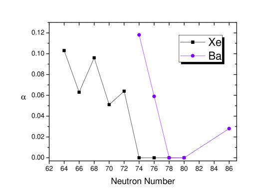
Figure 1: Values of $a$ for Xe and Ba isotopes, data taken from DDM .

Contraction process Gilmore examines the $Q_{u0}$ (12) at the north pole of $S_{5}$, where $q^{0}=\frac{1}{\sqrt{4a}}$ and the rest $q^{u}=0$,

$$Q_{uo}=-\frac{1}{\sqrt{4a}}\partial_{u}.$$ (20)

This expression is singular for $a=0$. Define the operator

$$\tilde{Q}_{u0}=\sqrt{4a}(q^{u}\partial_{0}-q^{0}\partial_{u}).$$ (21)

Now at the north pole and for $a=0$, $\tilde{Q}_{u0}=-\partial_{m}$. The set of generators $\{Q_{uk},\tilde{Q}_{u0}\}$ contracts to the set $\{{Q_{mn},\partial_{m}}\}$ for $a=0$. The latter set generates the $E(5)$ symmetry group Caprio , which was proposed in Iachello to characterize the critical point for a second order shape-phase transition from spherical to $\gamma$-unstable nuclei. It corresponds to the infinite square well potential for the $\beta$ variable, in the initial Bohr Hamiltonian. The Hamiltonian (18) for $a=0$ coincides with that of $E(5)$ Iachello . Now, the geometrical limit of IBM IBM in its $U(5)-O(6)$ transitional region hosts a point for a second order phase transition. The presence of $E(5)$ for $a=0$, the $O(5)$ invariance during the projection, as well as the argument that the Hamiltonian (18) should not correspond to an exact $O(6)$ limit, imply its adaptation to the $U(5)-O(6)$ transitional region of the IBM.

Predictions of $E(5)$ manifestations in atomic nuclei which lean on the spectrum of the initial Bohr Hamiltonian, are rather incomplete. The absence of the conformal factor in the initial Bohr Hamiltonian reflects the absence of $O(6)$ fingerprints. Parameter $a$ controls the presence of the conformal factor. In DDM , $a$-values are obtained by their rms fitting to the experimental data for the energy spectrum of a plethora of $\gamma$-unstable nuclei. A close examination of its available values draws attention to the nuclei for which $a=0$. Fig. 1 displays the a-values for the Xe and Ba isotopes. Parameter $a$ is not zero for a single nucleus in the series of Xe, or in that of the Ba isotopes. $a=0$ corresponds to the series of ¹²⁸ Xe, ¹³⁰ Xe, ¹³² Xe, ¹³⁴ Xe as well as in those of ¹³⁴ Ba and ¹³⁶ Ba. This remark should not be received as a proposal for $E(5)$ candidates. In DDM for $a=0$ the Hamiltonian of $E(5)$ Iachello is not obtained, Davidson term $\beta^{2}$ survives which nevertheless has been proposed to characterize the transitional region Rowe . The present approach implies that the manifestation of $E(5)$ in atomic nuclei, needs additional experimental measures than those obtained by the initial Bohr Hamiltonian. A geometrical limit of the IBM containing the parameter $a$ should illustrate its appearance in nuclear structure.

VI Conclusions

Beginning from a formal correspondence of Bohr space with the conformal factor and the cosmological Robertson-Walker geometry, Bohr model is embedded in six dimensions. The original Bohr space is located at the limit of infinite radius of a five sphere. Bohr Hamiltonian is re-formulated on the five sphere, which has the $O(6)$ symmetry group. Its relation with the $O(6)$ limit of the IBM indicates that the infinity of the five sphere corresponds to the limit of infinite number of bosons in the IBM.

The five sphere with finite radius corresponds to a constraint on the Number operator of the IBM. Bohr space with the conformal factor coincides with the stereographic projection of the five sphere on to the tangent plane. The re-formulation of the Bohr Hamiltonian on the projected plane is adapted to the $U(5)-O(6)$ region of the IBM. Its consequences are:

(i) The appearance of a deformation-dependent mass parameter in the original Bohr model.

(ii) Equivalently, in the projected plane the moments of inertia exhibit a different dependence with respect to the deformation, than in the original Bohr model. This implies the existence of symmetry-dependent rules for the relation of the moments of inertia with the intrinsic quadrupole moment.

(iii) In the limit of infinite radius of the five sphere, $E(5)$ Hamiltonian emerges. The new way of $E(5)$ generation challenges a discussion about its possible manifestations in atomic nuclei.

- (1) A. Bohr and B. Mottelson, Dan. Mat. Fys. Medd. 30, (1955), 1.
- (2) W. Greiner and J.A. Maruhn, Nuclear Models Springer-Verlag, Berlin, 1996.
- (3) A. Bohr, Dan. Mat. Fys. Medd. 26, (1952), 14.
- (4) F. Iachello and A. Arima, The Interacting Boson Model Cambridge University Press, Cambridge, 1987.
- (5) A.E.L. Dieperink, O. Scholten and F. Iachello, Phys. Rev. Lett. 44, (1980), 1747. J. N. Ginocchio and M. W. Kirson, Phys. Rev. Lett. 44, (1980), 1744.
- (6) P. Cejnar, J. Jolie and R. F. Casten, Rev. Mod. Phys., 82, (2010).
- (7) R. V. Jolos and P. von Brentano, Phys. Rev. C 79, (2009), 044310.
- (8) G. Scharff-Goldhaber, C.B. Dover and A.L. Goodman, Ann. Rev. Nucl. Sci. 26, (1976) 239-317.
- (9) P. Ring and P. Schuck, The Nuclear Many- Body Problem, Springer-Verlag, Berlin, 1980.
- (10) F. Iachello, Phys. Rev. Lett. 85, (2000), 3580.
- (11) D. Bonatsos, P.E. Georgoudis, D.Lenis, N.Minkov, and C.Quesne, Phys. Rev. C 83, (2011), 044321.
- (12) D.J. Rowe, T.A. Welsh and M.A. Caprio, Phys. Rev. C 79, (2009), 054304. See also David J.Rowe and John L.Wood, Fundamentals of Nuclear Models World scientific, London, 2009.
- (13) L.D. Landau and E.M. Lifshitz, The classical theory of fields, Butterworth-Heinemann, Oxford, 1999.
- (14) H.P. Robertson, Rev. Mod. Phys. 5, 62, (1933).
- (15) Robert Gilmore, Lie Groups, Lie Algebras and Some of their Applications, John Wiley and Sons, New York, 1974.
- (16) O. Castanos, E. Chacon, A. Frank and M. Moshinsky, J. Math. Phys. 20, (1979), 1.
- (17) M.A. Caprio and F. Iachello, Nucl. Phys. A781, (2007), 26.