Spin-Triplet Pairing State of Sr2RuO4 in the -Axis Magnetic Field
Shuhei TAKAMATSU1 and
Youichi YANASE1,2E-mail: takamatsu@phys.sc.niigata-u.ac.jp1Graduate School of Science and Technology1Graduate School of Science and Technology Niigata University Niigata University Niigata Niigata 950-2181 950-2181 Japan
2Department of Physics Japan
2Department of Physics Niigata University Niigata University Niigata Niigata 950-2181 950-2181 Japan Japan
Abstract
We investigate the spin-triplet superconducting state of Sr2RuO4
in the magnetic field along the c-axis on the basis of the four-component
Ginzburg-Landau (GL) model with a weak spin-orbit coupling.
We consider superconducting states described by the d-vector parallel to the ab-plane
(), and find that three spin-triplet pairing states
are stabilized in the magnetic field-temperature (-) phase diagram.
Although a helical state is stable at low magnetic fields, a chiral II state
is stabilized at high magnetic fields.
A non-unitary spin-triplet pairing state appears near the transition temperature owing to the
coupling of magnetic field and chirality.
We elucidate synergistic and/or competing roles of the magnetic field, chirality, and
spin-orbit coupling.
It is shown that a fractional vortex lattice is stabilized in the chiral II phase
owing to the spin-orbit coupling.
Since the discovery of superconductivity in Sr2RuO4 by Maeno et al.,[1]
extensive studies have been carried out to clarify the symmetry of superconductivity in Sr2RuO4.
It has been shown that Sr2RuO4 is a spin-triplet superconductor from both theoretical
and experimental points of view.[2, 3]
For instance, the Knight shift measurement by nuclear magnetic resonance (NMR) experiments is
one of the convincing piece of evidence of the spin-triplet pairing state.
The NMR measurements showed the temperature-independent Knight shift through the superconducting transition
in both field directions along the ab-plane[4] and along
the c-axis.[5]
These results indicate a spin-triplet superconducting state with
a d-vector perpendicular to the magnetic field.
This means that the “spin-orbit coupling” of spin-triplet Cooper pairs is very weak in Sr2RuO4.
According to the experiments of muon spin rotation (SR)[6] and
the Kerr effect,[7] the time reversal symmetry is spontaneously broken in
the superconducting state.
These findings indicated that the chiral spin-triplet pairing state described by the d-vector
is stabilized at zero magnetic field.
When the spin-orbit coupling is weak as indicated by NMR measurement[4, 5]
and by theoretical estimation[8],
the d-vector is rotated by a magnetic field along the c-axis
so as to be parallel to the ab-plane.
However, most theoretical studies focused on the chiral state
[9, 10, 11, 12, 13, 14, 15, 16, 17, 18]
assuming that a strong spin-orbit coupling pins the direction of the d-vector.
It is highly desired to investigate pairing states in the c-axis magnetic field
by taking a weak spin-orbit coupling into account, but no such theoretical study has yet been conducted.
The purpose of our study is to determine the spin-triplet superconducting state for
in the presence of a weak spin-orbit coupling.
Several issues regarding the superconductivity in Sr2RuO4 remain unsettled.
For instance, the chiral edge state[19] has not been observed[20],
and the first-order superconducting transition at high magnetic fields along the ab-plane [21]
is incompatible with the weak-coupling theory for spin-triplet superconductors.
To resolve these unresolved issues, our verification of superconducting phases
for will provide a basis for discussion.
Our study would also give an insight into the spin-triplet superconducting state of
UPt3[22], in which a weak spin-orbit coupling has been indicated[23].
We here construct a four-component GL model assuming a weak spin-orbit coupling.
Although the chiral state may be stabilized
at zero magnetic field[2, 3],
we assume that the d-vector is parallel to the ab-plane in the magnetic field along the c-axis
so as to gain the magnetic energy.
Focusing on this high-field superconducting phase,
we take into account two spin components of order parameters,
namely, and .
The D4h symmetry of the crystal structure of Sr2RuO4 allows two orbital components
of -wave order parameters, namely, and , which are equivalently
denoted by the chirality, that is, .
These component order parameters correspond to
four irreducible representations in the D4h symmetry,
and
[24].
These pairing states are nearly degenerate when we assume a weak spin-orbit coupling.
For convenience, we describe the order parameters as
using four component order parameters, .
and stand for pairing functions with
the same symmetry as and under the D4h point group, respectively.
The GL free-energy density is given by
(1)
where is the same as the GL free-energy density for the Eu representation
of the tetragonal point group[24],
(2)
We adopt , where is the transition temperature
at zero magnetic field in the absence of spin-orbit coupling.
We use the conventional notation
and .
In the weak coupling theory, parameters satisfy the relations following
,
,
and ,
where and are the Fermi velocity and
brackets denote the average over the Fermi surface.
When we assume , we obtain .
On the other hand, we find for the pairing functions obtained by a perturbation theory
for the Hubbard model[25].
A weak spin-orbit coupling is taken into account in the quadratic terms
and , which are given by
(3)
(4)
According to a theoretical analysis based on the three-orbital Hubbard model
for Sr2RuO4[8], the term arises from the -bands,
while the term is due to the coupling between the -bands
and the -band.
We determine the pairing state by minimizing the above GL free-energy density
using the variational method.
We take into account variational wave functions of Cooper pairs so that the solution of
the linearized GL equation is reproduced.
Writing
and
,
and differentiating the quadratic terms of eq. (2) with respect to
and , we obtain the linearized GL equation
in the absence of spin-orbit coupling as
(9)
(12)
where , , and
.
Note that this equation is independent of the spin label .
For ,
the minimum eigenvalue is obtained for the pairing state
with a positive chirality, in which the order parameters
are described using the Landau level expansion
(13)
The superconducting transition temperature in the absence of spin-orbit coupling is obtained as
. The pairing state with a negative chirality
is described by another eigenstate of the linearized GL equation as
(14)
We here denote the n-th Landau level wave functions
and
using the unit of length and the Hermite polynomials .
We here assume the square lattice structure of the vortex
in accordance with the small-angle neutron scattering experiment[26].
Thus, we take for all integers and .
We adopt variational wave functions consisting of a linear combination of
the above solutions of the linearized GL equation:
(21)
(28)
where and ( and ) represent Cooper pairs with up spin (down spin)
and dominantly positive and negative chiralities, respectively.
Two-dimensional vectors determine the position of vortex cores.
We take without any loss of generality.
These variational wave functions precisely reproduce the pairing state
near the transition temperature, and their validity at low temperatures
has been justified by the calculation for the chiral superconducting state[11].
Substituting eqs. (13)-(28)
into eqs. (2)-(4) and
integrating over the unit cell,
we obtain the free-energy density as
(29)
where is the area of a unit cell.
Variational parameters are
optimized to minimize the GL free-energy density.
We find that and
in the following results.
In the following, we choose the parameters , and using .
For spin-orbit couplings, we assume and
unless explicitly mentioned otherwise.
We assume the sign and so that a helical state with the d-vector
is stabilized at zero magnetic field.
Later, we will discuss the other cases and show that the following results are not altered
by the sign of and .
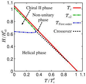
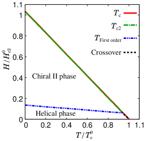
Figure 1 shows the result of the - phase diagram.
We see that the helical state is stable at low magnetic fields, while
the “chiral II state” is stabilized for .
The d-vector of the chiral II state is approximately described as
, or ,
which is different from in the chiral state.
It is shown that the superconducting double transitions occur at high magnetic fields,
the chiral II state changes to the non-unitary state near the transition temperature.
This non-unitary state changes to the helical state at low magnetic fields through the crossover.
The chiral state may be stabilized near the
zero magnetic field[2, 3],
but we do not show this in Fig. 1.
Figure 1: (Color online) The - phase diagram of four-component GL model [eq. (1)]
for , and .
The unit of magnetic field is .
The red solid line shows the superconducting transition temperature ,
while the green dot-dashed line shows the second superconducting transition temperature .
The blue double-dot-dashed line and black dashed line depict the first-order transition
and crossover, respectively. We define the crossover temperatures as .
The non-unitary phase, helical phase, and chiral II phase depicted in the phase diagram
are approximately described by the d-vector
,
,
and , respectively,
for our choice of parameters , and .
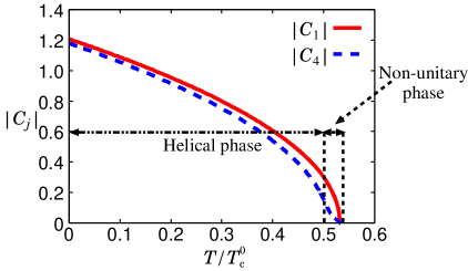
The other cases are summarized in Tables I and II.Figure 2: (Color online) Temperature dependence of the absolute values of
variational parameters at .
The other parameters are the same as those in Fig. 1.
We show (red solid line) and (blue dashed line), since .
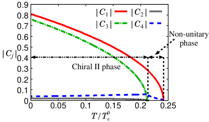
We define the crossover temperature as .Figure 3: (Color online)
Temperature dependence of the absolute values of
variational parameters (red solid line), (black dotted line),
(green dot-dashed line), and
(blue dashed line) at .
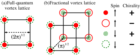
The other parameters are the same as those in Fig. 1.Figure 4: (Color online) Schematic figure of vortex lattices.
(a) Full-quantum vortex lattice in the non-unitary and helical phases.
(b) Fractional vortex lattice in the chiral II phase.
Vortex cores of (red closed circles), (red open circles),
(green shaded circles),
and (green open circles with dashed lines) terms are depicted.
The spin and chirality of each component are shown on the right-hand side of figures.
We choose the unit of length .
To clarify these pairing states, we show the temperature dependence of
variational parameters. Figure 2 shows the absolute values
at an intermediate magnetic field .
We see that and are finite, but in the helical state
and non-unitary state.
Although and have nearly the same magnitude in the helical state,
near the transition temperatures, indicating
the non-unitary spin-triplet superconducting state with
.
Later, we will show that the other non-unitary state
is stabilized for a positive spin-orbit coupling .
Note that the non-unitary state is stabilized
by the spin-orbit coupling and orbital pair breaking effect in this case.
This mechanism of stabilizing the non-unitary state is different from the conventional one,
which realizes the phase of superfluid 3He [27]
and possibly Sr2RuO4.[25]
We elucidate this ”orbital-induced non-unitary state” by looking at the chirality in
each spin component of Cooper pairs.
For , the Cooper pairs formed by quasiparticles
with up spin have the positive chirality as ,
while the chirality is negative for down spin as .
When the magnetic field is switched on, the positive chirality is enhanced by the coupling of
chirality and magnetic field.[9]
Thus, the dominant order parameter is
in the non-unitary state, although a subdominant order parameter
is induced by the spin-orbit coupling.
Note that the cooperation of the chirality, magnetic field, and spin-orbit coupling plays
an essential role in stabilizing this orbital-induced non-unitary state.
Figure 3 shows the variational parameters
at a rather high magnetic field .
We see that the parameter has a large magnitude in the low-temperature chiral II phase.
This is because the magnetic field favors the positive chirality of Cooper pairs
with down spin .
This coupling of chirality and magnetic field competes with the spin-orbit coupling,
which stabilizes the negative chirality of .
The former is more important than the latter at high fields, and therefore stabilizes the
chiral II phase.
On the other hand, the negative chirality component
, which is represented by ,
is suppressed in the chiral II state.
Taking the and terms into account, the chiral II state is
described by the d-vector or
.
These two pairing states are degenerate because the spin-orbit coupling terms
between and cancel out.
In other words, Cooper pairs with up spin
are almost decoupled from those with down spin
in the chiral II phase.
This unusual decoupling leads to the fractional vortex lattice, which we discuss below.
Chiral II phase
Non-unitary phase
Table 1: Summary of d-vector in the non-unitary phase and chiral II phase.
The magnitude relation between and determines the chirality.
The spin component in the non-unitary phase is determined by the sign of spin-orbit coupling .
Helical phase
Table 2: Summary of d-vector in the helical phase.
The sign of spin-orbit couplings and determines the d-vector.
We now turn to the vortex lattice structure.
Interestingly, we find that the fractional vortex lattice
appears in the chiral II phase in contrast to the conventional full-quantum vortex lattices
in the non-unitary and helical phases.
We schematically illustrate these vortex lattices in Fig. 4.
It is shown that the vortex cores of order parameters for
() and for
()
shift from those of ()
and ().
Thus, a core-less vortex is stabilized in the chiral II phase, which is regarded as
a fractional vortex lattice state[28].
Note that this fractional vortex lattice is stabilized by the spin-orbit coupling,
in sharp contrast to the usual role of spin-orbit coupling.
When we assume a strong spin-orbit coupling, the fractional vortex lattice is destabilized so that
the spin-orbit coupling energy is gained[28].
Contrary to this common knowledge, the role of spin-orbit coupling is altered in the chiral II phase
because of the chirality arising from two orbital components.
We will show details of the fractional vortex lattice structure in another paper.
Here, we investigate the parameter dependences of the phase diagram.
We would like to stress again that the structure of the phase diagram is not altered by
the signs of the spin-orbit couplings and or by the magnitude
relation .
When we change the sign of these parameters, the d-vector in each phase changes
as summarized in Tables 1 and 2.
The magnitude relation between and determines the chirality (Table 1).
On the other hand, the signs of the spin-orbit couplings and determine
the d-vector of the helical phase (Table 2).
The spin component in the non-unitary phase is also determined by the sign of
(Table 1).
When the magnitude of spin-orbit couplings is decreased, the chiral II phase is stabilized.
Figure 5 shows that the chiral II phase is stable in almost the entire
parameter range of the - phase diagram for tiny spin-orbit couplings,
and .
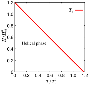
On the other hand, moderate spin-orbit couplings, and ,
stabilize the helical phase in the entire parameter range, as shown in Fig. 6.
In both cases, the vortex lattice structure is not altered from Fig. 4.
A microscopic calculation based on the three-orbital Hubbard model
has estimated these parameters as [8].
Thus, the moderate spin-orbit couplings assumed in Fig. 6 are not likely realized
in Sr2RuO4.
Figure 5: (Color online) - phase diagram for and
.
The other parameters are the same as those in Fig. 1.Figure 6: (Color online) - phase diagram for and .
The other parameters are the same as those in Fig. 1.
Finally, we discuss the pairing state in Sr2RuO4 on the basis of our results in
Figs. 1, 5, and 6.
Until now, double superconducting transitions have not been observed in Sr2RuO4
in the magnetic field along the c-axis[2, 3].
This experimental status implies tiny spin-orbit couplings as in Fig. 5
or moderate spin-orbit couplings as in Fig. 6.
The chiral II state is realized in the former case,
while the helical state is realized in the latter case.
The latter interpretation is, however, incompatible with the results of the NMR experiment,
which did not show any temperature dependence of
Knight shift through [4, 5].
On the other hand, the case of tiny spin-orbit couplings in Fig. 5 seems to
be consistent with the experiments. Although the fractional vortex lattice in
Fig. 4(b) has not been observed in the small-angle neutron scattering
experiment[26], this discrepancy is not a serious issue because the fractional
vortex lattice is affected by the strong coupling effect as well as by the Meissner effect.
In our future study, we will investigate these effects on the vortex lattice structure.
In contrast to these cases, the multiple-phase diagram as shown in Fig. 1
should appear in Sr2RuO4 when spin-orbit couplings are small but not tiny.
No clear experimental observation has been reported for the multiple-phase diagram.
However, weak evidence has been obtained by a small-angle neutron scattering experiment[26].
When the fractional vortex lattice is realized in the chiral II phase, the spatial distribution
of the magnetic field is smeared, consistent with the unclear field distribution
obtained in an experiment at high magnetic fields[26].
Further experimental study is desired to determine the superconducting state of
Sr2RuO4 in the c-axis magnetic field.
In summary, we studied the spin-triplet superconducting state of Sr2RuO4 in the magnetic
field along the c-axis. We assumed a weak spin-orbit coupling of Cooper pairs and considered
the d-vector parallel to the ab-plane.
We determined multiple phases against magnetic fields and temperatures by analyzing
the four-component GL model using the variational method.
Interestingly, we showed three spin-triplet superconducting phases, which are orbital-induced
non-unitary phase, chiral II phase, and helical phase.
We clarified the synergistic and competing roles of the chirality, magnetic field,
and spin-orbit coupling for these pairing states.
We would like to stress that these intriguing superconducting phases are obtained
because we take into account a weak but finite spin-orbit coupling and allow the mixing of
irreducible representations in the order parameters.
We also found that the fractional vortex lattice is stabilized by a weak spin-orbit coupling
in the chiral II phase.
This is in sharp contrast to the theory of non-chiral spin-triplet superconductors[28].
This finding pave the way for realizing a novel topological defect with Majorana fermion[29]
in spin-triplet superconductors with spin and orbital degrees of freedom.
The authors are grateful to K. Ishida, Y. Maeno, Y. Matsuda, S. Yonezawa, and S. Kashiwaya
for fruitful discussions.
We especially thank M. Sigrist for stimulating discussions on the spin-triplet superconductivity.
This work was supported by KAKENHI (Grant Nos. 24740230 and 23102709).
References
[1]
Y. Maeno, H. Hashimoto, K. Yoshida, S. Nishizaki, T. Fujita, J. G. Bednorz, and F. Lichtenberg:
Nature 372 (1994) 532.
[2]
A. P. Mackenzie and Y. Maeno:
Rev. Mod. Phys. 75 (2003) 657.
[3]
Y. Maeno, S. Kittaka, T. Nomura, S. Yonezawa, and K. Ishida:
J. Phys. Soc. Jpn. 81 (2012) 011009.
[4]
K. Ishida, H. Mukuda, Y. Kitaoka, K. Asayama, Z. Q. Mao, Y. Mori, and Y. Maeno:
Nature 396 (1998) 658.
[5]
H. Murakawa, K. Ishida, K. Kitagawa, H. Ikeda, Z. Q. Mao, and Y. Maeno:
Phys. Rev. Lett. 93 (2004) 167004.
[6]
G. M. Luke, Y. Fudamoto, K. M. Kojima, M. I. Larkin, J. Merrin, B. Nachumi, Y. J. Uemura,
Y. Maeno, Z. Q. Mao, Y. Mori, H. Nakamura, and M. Sigrist:
Nature 394 (1998) 558.
[7]
J. Xia, Y. Maeno, P. T. Beyersdorf, M. M. Fejer, and A. Kapitulnik:
Phys. Rev. Lett. 97 (2006) 167002.
[8]
Y. Yanase and M. Ogata: J. Phys. Soc. Jpn. 72 (2003) 673.
[9]
D. F. Agterberg: Phys. Rev. Lett. 80 (1998) 5184.
[10]
D. F. Agterberg: Phys. Rev. B 58 (1998) 14484.
[11]
T. Kita: Phys. Rev. Lett. 83 (1999) 1846.
[12]
Y. Kato: J. Phys. Soc. Jpn. 69 (2000) 3378.
[13]
Y. Kato and N. Hayashi: J. Phys. Soc. Jpn. 70 (2001) 3368.
[14]
M. Takigawa, M. Ichioka, K. Machida, and M. Sigrist:
Phys. Rev. B 65 (2001) 014508.
[15]
M. Ichioka and K. Machida: Phys. Rev. B 65 (2002) 224517.
[16]
J. Garaud, D. Agterberg, and E. Babaev: Phys. Rev. B 86 (2012) 060513(R).
[17]
M. A. Silaev: arXiv:1301.6146.
[18]
J.-W. Huo and F.-C. Zhang: Phys. Rev. B 87 (2013) 134501.
[19]
M. Matsumoto and M. Sigrist: J. Phys. Soc. Jpn. 68 (1999) 994.
[20]
For a review, C. Kallin: Rep. Prog. Phys. 75 (2012) 042501.
See also, Y. Imai, K. Wakabayashi, and M. Sigrist: Phys. Rev. B 85 (2012) 174532.
[21]
S. Yonezawa, T. Kajikawa, and Y. Maeno: Phys. Rev. Lett. 110 (2013) 077003.
[22]
For a review, R. Joynt and L. Taillefer: Rev. Mod. Phys. 74 (2002) 235.
[23]
H. Tou, Y. Kitaoka, K. Asayama, N. Kimura, Y. Onuki, E. Yamamoto, and K. Maezawa:
Phys. Rev. Lett. 77 (1996) 1374;
H. Tou, Y. Kitaoka, K. Ishida, K. Asayama, N. Kimura, Y. Onuki, E. Yamamoto,
Y. Haga, and K. Maezawa: Phys. Rev. Lett. 80 (1998) 3129.
[24]
M. Sigrist and K. Ueda: Rev. Mod. Phys. 63 (1991) 239.
[25]
M. Udagawa, Y. Yanase, and M. Ogata: J. Phys. Soc. Jpn. 74 (2005) 2905.
[26]
T. M. Riseman, P. G. Kealy, E. M. Forgan, A. P. Mackenzie, L. M. Galvin, A. W. Tyler,
S. L. Lee, C. Ager, D. McK. Paul, C. M. Aegerter, R. Cubitt, Z. Q. Mao, T. Akima, and Y. Maeno:
Nature 396 (1998) 242; 404 (2000) 629.
[27]
A. J. Leggett: Rev. Mod. Phys. 47 (1975) 331.
[28]
S. B. Chung, D. F. Agterberg, and E.-A. Kim: New J. Phys. 11 (2009) 085004.
[29]
D. A. Ivanov: Phys. Rev. Lett. 86 (2001) 268.