Time-Energy Measure for Quantum Processes

Abstract

Quantum mechanics sets limits on how fast quantum processes can run given some system energy through time-energy uncertainty relations, and they imply that time and energy are tradeoff against each other. Thus, we propose to measure the time-energy as a single unit for quantum channels. We consider a time-energy measure for quantum channels and compute lower and upper bounds of it using the channel Kraus operators. For a special class of channels (which includes the depolarizing channel), we can obtain the exact value of the time-energy measure. One consequence of our result is that erasing quantum information requires $\sqrt{(n+1)/n}$ times more time-energy resource than erasing classical information, where $n$ is the system dimension.

I Introduction

Evolution of quantum processes (including performing quantum computation) requires physical resources, in particular, time and energy. The computation speed of a physical device is governed by physical laws and is limited by the energy of the device. Under the constraints of quantum mechanics, system evolutions are bounded by time-energy uncertainty relations (TEURs) Lloyd (2000). The investigation of TEURs has a long history. The first major result of a TEUR was proved by Mandelstam and Tamm Mandelstam and Tamm (1945). This was followed by subsequent work on isolated systems  Bhattacharyya (1983); Anandan and Aharonov (1990); Uhlmann (1992); Vaidman (1992); Pfeifer (1993); Margolus and Levitin (1996, 1998); Chau (2010) and composite systems with entanglement Giovannetti et al. (2003a, b); Zander et al. (2007). Recently, TEURs for general quantum processes have also been proved Taddei et al. (2013); del Campo et al. (2013). The general form of TEURs is an inequality that sets a lower limit on the product of the system energy (or a function of the energies) and the time it takes to evolve an initial state to a final state (e.g., an orthogonal state). Motivated by the TEURs and recognizing that time and energy are tradeoff against each other, time-energy can be regarded as a single property of a quantum process. The intuition is that the more computation or work a quantum process performs, the more time-energy it requires. And it is up to the system designer (or nature) to perform it with more time but less energy, or vice versa. Thus, our goal in this paper is to investigate the time-energy requirements of quantum processes by using a time-energy measure. Chau Chau (2011) proposed a time-energy measure for unitary transformations that is based on a TEUR proved earlier Chau (2010). In this paper, we extend this measure to quantum processes. The TEUR due to Chau Chau (2010) is tight in the sense that it can be saturated by some states and Hamiltonians, and thus it serves to motivate a good definition for a time-energy measure. To see this, let’s start with this TEUR. Given a time-independent Hamiltonian $H$ of a system, the time $t$ needed to to evolve a state $\left|\Phi\right\rangle$ under the action of $H$ to a state whose fidelity  is less than or equal to $\epsilon$ satisfies the TEUR

$$t\geq\frac{(1-\sqrt{\epsilon})\hbar}{A\sum_{j}|\alpha_{j}|^{2}|E_{j}|}$$ (1)

where $E_{j}$’s are the eigenvalues of $H$ with the corresponding normalized energy eigenvectors $\left|E_{j}\right\rangle$’s, $\mbox{$\left|\Phi\right\rangle$}=\sum_{j}\alpha_{j}\mbox{$\left|E_{j}\right\rangle$}$, and $A\approx 0.725$ is a universal constant. Essentially, after time $t$, the state transforms unitarily according to $U=e^{-iHt/\hbar}$. The same $U$ could be implemented with either a high energy $H$ run for a shorter time or a low energy $H$ run for a longer time. Based on Eq. (1), a weighted sum of $|tE_{j}|$’s serves as an indicator of the time-energy resource needed to perform $U$, and as such the following time-energy measure on unitary matrices was proposed by Chau Chau (2011):

$$\lVert U\rVert_{\vec{\mu}} =\sum_{j=1}^{r}\mu_{j}|\theta_{j}|^{\downarrow}$$

where $U$ has eigenvalues $\exp(-iE_{j}t/\hbar)\equiv\exp(\theta_{j})$ and $\vec{\mu}$ is some fixed vector to be described later (see Sec. II). In essence, a large value of $\lVert U\rVert_{\vec{\mu}}$ suggests that a long time may be needed to run a Hamiltonian that implements $U$ for a fixed energy, and vice versa.

In this paper, we are interested in an analogous measure for quantum channels which include unitary transformations as special cases. We are given a quantum channel $\mathcal{F}(\rho)$ acting on system $A$ that maps $n\times n$ density matrix $\rho$ to another one with the same dimension. There exist unitary extensions $U_{BA}$ in a larger Hilbert space with an ancillary system $B$ such that $\mathcal{F}(\rho)={\rm Tr}_{B}[U_{BA}(\mbox{$\left|0\right\rangle$}_{B}\mbox{$\left\langle 0\right|$}\otimes\rho_{A})U_{BA}^{\dagger}]$. Each $U_{BA}$ could have a different time-energy spectrum and we want to select the one requiring the least resource for $\mathcal{F}$. We extend the resource indicator for $U$ to quantum channel $\mathcal{F}$ by defining

$$\halign to=0.0pt{ \hfil$\displaystyle{#}$&\hfil$\displaystyle{{}#{}}$\hfil&\hfil$\displaystyle{{}#{}}$\hfil&$\displaystyle{#}$\hfil&\refstepcounter{equation}\label{#}\llap{(\theequation)}\cr\vskip-6.0pt\cr\lVert\mathcal{F} \rVert_{\vec{\mu}} &\equiv&\min_{U} &\lVert U \rVert_{\vec{\mu}} \cr&&\text{s.t.} &\mathcal{F}(\rho) = {\rm Tr}_{B} [ U_{BA} (\mbox{$\left|0\right\rangle$}_{B}\mbox{$\left\langle 0\right|$} \otimes\rho_{A}) U_{BA}^{\textdagger}] \> \forall\rho. \cr}$$

This gives a $U$ that consumes the least time-energy resource. Thus, $\lVert\mathcal{F}\rVert_{\vec{\mu}}$ is an indicator of the resource needed to perform $\mathcal{F}$. We formally formulate this problem in Sec. II into the “partial $U$ problem” and the “channel problem”. Then, we simplify the “partial $U$ problem” in Sec. III and solve the a special case of it in Sec. IV. The special case solution will be used to prove our major results which are the upper bound of the time-energy resource measure $\lVert\mathcal{F}\rVert_{\vec{\mu}}$ (Sec. V), the lower bound of $\lVert\mathcal{F}\rVert_{\vec{\mu}}$ (Sec. VI), and the optimal $\lVert\mathcal{F}\rVert_{\vec{\mu}}$ for a class of quantum channels (Sec. VII). The lower- and upper-bounds of the time-energy $\lVert\mathcal{F}\rVert_{\vec{\mu}}$ hold for any quantum channel $\mathcal{F}$ and for specific $\vec{\mu}$:

$$\lVert\mathcal{F}\rVert_{\text{max}} \geq\min_{\mathbf{v}:\>\lVert\mathbf{v}\rVert\leq 1}\>\max_{1\leq i\leq n}\cos^{-1}\Big{[}\operatorname{Re}(\lambda_{i}(\sum_{j=1}^{d}v_{j}F_{j}))\Big{]}$$ (2)

$$\lVert\mathcal{F}\rVert_{\text{max}} \leq\min_{\mathbf{v}:\>\lVert\mathbf{v}\rVert\leq 1}\sum_{i=1}^{n}\cos^{-1}\Big{[}\operatorname{Re}(\lambda_{i}(\sum_{j=1}^{d}v_{j}F_{j}))\Big{]}$$ (3)

$$\lVert\mathcal{F}\rVert_{\text{sum}} \geq\min_{\mathbf{v}:\>\lVert\mathbf{v}\rVert=1}\>\max_{1\leq i\leq n}2\cos^{-1}|\lambda_{i}(\sum_{j=1}^{d}v_{j}F_{j})|$$ (4)

$$\lVert\mathcal{F}\rVert_{\text{sum}} \leq\min_{\mathbf{v}:\>\lVert\mathbf{v}\rVert\leq 1}\sum_{i=1}^{n}2\cos^{-1}\Big{[}\operatorname{Re}(\lambda_{i}(\sum_{j=1}^{d}v_{j}F_{j}))\Big{]}$$ (5)

where $\lVert\mathbf{v}\rVert=\sqrt{\sum_{j=1}^{d}|v_{j}|^{2}}$, $F_{j}\in{\mathbb{C}}^{n\times n},j=1,\dots,d$ are the Kraus operators of $\mathcal{F}$, and $\lambda_{i}(\cdot)$ denotes the $i$th eigenvalue of its argument. Here, $\lVert\cdot\rVert_{\text{max}}$ is a short-hand notation for $\lVert\cdot\rVert_{\vec{\mu}}$ with $\vec{\mu}=[1,0,0,\dots]$ and $\lVert\cdot\rVert_{\text{sum}}$ for $\lVert\cdot\rVert_{\vec{\mu}}$ with $\vec{\mu}=[1,1,1,\dots]$. For a class of channels (which includes the depolarizing channel), we obtain the exact value for $\lVert\mathcal{F}\rVert_{\text{max}}$ in Sec. VII. In particular, when $\mathcal{F}$ is a depolarizing channel with probability $q$ that the input state is unchanged, its time-energy requirement is $\lVert\mathcal{F}\rVert_{\text{max}}=\cos^{-1}\sqrt{q+(1-q)/n^{2}}$. Finally, in Sec. VIII, we study the time-energy resource needed to erase information in both the quantum and classical settings. We conclude that $\sqrt{(n+1)/n}$ times more resource is required in the quantum setting than in the classical setting and that the amount of time-energy resource needed for $k$ runs of the depolarizing channel scales as $\sqrt{k}$ when the noise is small.

II Problem formulation

II.1 Notations and assumptions

We can describe $\mathcal{F}(\rho)$ using the Kraus operators: $\mathcal{F}(\rho)=\sum_{j=1}^{d}F_{j}\rho F_{j}^{\dagger}$ where $F_{j}\in{\mathbb{C}}^{n\times n}$ are the Kraus operators satisfying the trace-preserving condition $\sum_{j=1}^{d}F_{j}^{\dagger}F_{j}=I$. Note that any channel can be described by at most $n^{2}$ Kraus operators. But here the formulation is general for any number of Kraus operators.

Denote by $\operatorname{U}(r)$ the group of $r\times r$ unitary matrices.

Decompose $U\in\operatorname{U}(r)$ into eigenvectors:

$$U=\sum_{j=1}^{r}\exp(-i\theta_{j})\mbox{$\left|u_{j}\right\rangle$}\mbox{$\left\langle u_{j}\right|$}$$ (6)

where $\theta_{j}=E_{j}t/\hbar$, $E_{j}$ is the energy, and $t$ is the evolution time. We call $\theta_{j}$’s eigenangles. We assume that all angles are taken in the range $(-\pi,\pi]$. Define a time-energy measure for $U$ Chau (2011)

$$\lVert U\rVert_{\vec{\mu}} =\sum_{j=1}^{r}\mu_{j}|\theta_{j}|^{\downarrow}$$ (7)

where $|\theta_{j}|^{\downarrow}$ denotes $|\theta_{j}|$ ordered non-increasingly $|\theta_{1}|^{\downarrow}\geq|\theta_{2}|^{\downarrow}\geq\cdots\geq|\theta_{r}|^{\downarrow}$. Also, $\vec{\mu}=[\mu_{1},\mu_{2},\dots,\mu_{r}]\neq\vec{0}$ with $\mu_{1}\geq\mu_{2}\geq\cdots\geq\mu_{r}\geq 0$. Note that $\lVert U\rVert_{\vec{\mu}}$ satisfies the multiplicative triangle inequality $\lVert UV\rVert_{\vec{\mu}}\leq\lVert U\rVert_{\vec{\mu}}+\lVert V\rVert_{\vec{\mu}}$ Chau (2011).

We have two special cases for the time-energy measure:

$\bullet$ Sum time-energy:	$\lVert U\rVert_{\text{sum}}\equiv\displaystyle\sum_{j=1}^{r}|\theta_{j}|$ .	$(8)$
$\bullet$ Max time-energy:	$\lVert U\rVert_{\text{max}}\equiv\displaystyle\max_{1\leq j\leq r}|\theta_{j}|=|\theta_{1}|^{\downarrow}$.	$(9)$

Note that the subscript “sum” is short for $\vec{\mu}=[1,1,\dots,1]$ and “max” for $\vec{\mu}=[1,0,\dots,0]$.

Define $\lVert\mathbf{v}\rVert=\sqrt{\sum_{j=1}^{d}|v_{j}|^{2}}$ where $\mathbf{v}=[v_{1},v_{2},\dots,v_{d}]$.

We adopt the convention that $\cos^{-1}$ always returns an angle in the range $[0,\pi]$.

II.2 The “partial $U$ problem” and the “channel problem”

We generalize the measure $\lVert\cdot\rVert_{\vec{\mu}}$ to the case where part of a unitary matrix is given. Suppose that we are given the first $n\leq r$ columns of $U$ denoted by $U_{[1,n]}\in{\mathbb{C}}^{r\times n}$. Define the “partial $U$ problem” for $U_{[1,n]}$:

$$\halign to=0.0pt{ \hfil$\displaystyle{#}$&\hfil$\displaystyle{{}#{}}$\hfil&\hfil$\displaystyle{{}#{}}$\hfil&$\displaystyle{#}$\hfil&\refstepcounter{equation}\label{#}\llap{(\theequation)}\cr\vskip-6.0pt\cr\lVert U_{[1,n]} \rVert_{\vec{\mu}} &\equiv&\displaystyle\min_{V} &\lVert V \rVert_{\vec{\mu}}\cr&&\text{s.t.}&V_{[1,n]}=U_{[1,n]}\text{ and}\cr&&&V \in\operatorname{U}(r).&\hbox to0.0pt{\hss(10\cr}}$$

We use this as a bridge to generalize the measure to quantum channel $\mathcal{F}(\rho_{A})$ acting on density matrix $\rho_{A}\in{\mathbb{C}}^{n\times n}$. For such a channel $\mathcal{F}(\rho_{A})=\sum_{i=1}^{d}F_{i}\rho_{A}F_{i}^{\dagger}$ where $F_{i}\in{\mathbb{C}}^{n\times n}$, there exist unitary extensions $U_{BA}$ in a larger Hilbert space with an ancillary system $B$ such that $\mathcal{F}(\rho_{A})={\rm Tr}_{B}[U_{BA}(\mbox{$\left|0\right\rangle$}_{B}\mbox{$\left\langle 0\right|$}\otimes\rho_{A})U_{BA}^{\dagger}]$.

Define a mapping from a sequence of Kraus operators $F_{1:{d}}\triangleq(F_{1},F_{2},\ldots,F_{d})$ to an ${d}{n}\times{n}$ matrix as follows:

$$g(F_{1:{d}}) \triangleq\begin{bmatrix}F_{1}\\ F_{2}\\ \vdots\\ F_{{d}}\end{bmatrix}.$$ (11)

Because $\sum_{j=1}^{{d}}F_{j}^{\dagger}F_{j}=I$, the columns of $g(F_{1:{d}})$ are orthonormal and $g(F_{1:{d}})$ can be regarded as a submatrix of a unitary one. Thus, we can obtain $\lVert g(F_{1:{d}})\rVert_{\vec{\mu}}$ from problem (II.2).

Note that two sets of Kraus operators $\{F_{1},\ldots,F_{d}\}$ and $\{F_{1}^{\prime},\ldots,F_{d}^{\prime}\}$ represent the same quantum channel if and only if $F_{i}^{\prime}=\sum_{j=1}^{d}w_{ij}F_{j}$ for all $i$ and for some unitary matrix $[w_{ij}]$ (see Ref. Nielsen and Chuang (2000)). If more Kraus operators are desired in one set, we can supplement the other set with all-zero Kraus operators. This implies that given one Kraus representation $\{F_{1},\ldots,F_{d}\}$, the most general form of all unitary extension implementing $\mathcal{F}$ is

$$U_{BA}=(W_{B}\otimes I_{A})\underbrace{\begin{bmatrix}F_{1}&*&*&\cdots&*\\ F_{2}&*&*&\cdots&*\\ \vdots&&&&\vdots\\ F_{d}&*&*&\cdots&*\\ \mathbf{0}&*&*&\cdots&*\\ \vdots&&&&\vdots\\ \mathbf{0}&*&*&\cdots&*\end{bmatrix}}_{\displaystyle\tilde{U}_{BA}}$$ (12)

where $W_{B}$ is any unitary of dimension $d^{\prime}\times d^{\prime}$, $I_{A}$ is the identity matrix of dimension $n\times n$, $\tilde{U}_{BA}$ is any unitary of dimension $nd^{\prime}\times nd^{\prime}$ with the first $n$ columns fixed as shown, and $\mathbf{0}$ is the all-zero matrix of dimension $n\times n$. Here, we allow $d^{\prime}$ to be in the range $d\leq d^{\prime}<\infty$.

We define the time-energy measure of the quantum channel $\mathcal{F}$ given a Kraus representation $\{F_{1},\ldots,F_{d}\}$ as follows:

$$\halign to=0.0pt{ \hfil$\displaystyle{#}$&\hfil$\displaystyle{{}#{}}$\hfil&\hfil$\displaystyle{{}#{}}$\hfil&$\displaystyle{#}$\hfil&\refstepcounter{equation}\label{#}\llap{(\theequation)}\cr\vskip-6.0pt\cr\lVert\mathcal{F} \rVert_{\vec{\mu}} &\equiv&\min_{W_{B},d'} &\lVert (W_{B} \otimes I_{A}) \tilde{U}_{BA}(1:n) \rVert_{\vec{\mu}}\cr&&\text{s.t.}&W_{B} \in\operatorname{U}(d')\text{ and }d \leq d' < \infty,&\hbox to0.0pt{\hss(13\cr}}$$

where we make use of Eq. (II.2) in the objective function and $\tilde{U}_{BA}(1:n)$ are the first $n$ columns of $\tilde{U}_{BA}$ given in Eq. (12). We call this the “channel problem”.

Our ultimate goal is to find the minimum time-energy required to implement a quantum channel by solving the “channel problem” (II.2). We first consider the “partial $U$ problem” (II.2).

III Simplification of the “partial $U$ problem”

The “partial $U$ problem” (II.2) can be recast as that given $U$ of dimension $r\times r$ of the form

$$U=\begin{bmatrix}\mbox{$\left|b_{1}\right\rangle$}&\mbox{$\left|b_{2}\right\rangle$}&\dots&\mbox{$\left|b_{n}\right\rangle$}&*&*&\cdots&*\end{bmatrix}$$ (14)

where the first $n$ columns, labeled as $\mbox{$\left|b_{i}\right\rangle$},i=1,\dots,n$, are fixed, our goal is to find the remaining $r-n$ columns to minimize $\lVert U\rVert_{\vec{\mu}}$ while maintaining $U$ unitary.

It is helpful to consider $U$ as a mapping with the requirement that it performs the following transformations:

$$\mbox{$\left|e_{i}\right\rangle$}\longrightarrow\mbox{$\left|b_{i}\right\rangle$}\>\>\text{for all }i=1,\ldots,n$$ (15)

where $\left|e_{i}\right\rangle$ is the unit vector with $1$ at the $i$th entry and $0$ everywhere else. Then, the “partial $U$ problem” (II.2) for $U_{[1,n]}$ is equivalent to

$$\halign to=0.0pt{ \hfil$\displaystyle{#}$&\hfil$\displaystyle{{}#{}}$\hfil&\hfil$\displaystyle{{}#{}}$\hfil&$\displaystyle{#}$\hfil&\refstepcounter{equation}\label{#}\llap{(\theequation)}\cr\vskip-6.0pt\cr\lVert U_{[1,n]} \rVert_{\vec{\mu}} &=&\displaystyle\min_{U} &\lVert U \rVert_{\vec{\mu}}\cr&&\text{s.t.}&U\mbox{$\left|e_{i}\right\rangle$} = \mbox{$\left|b_{i}\right\rangle$} \>\> \text{for all }i=1,\ldots,n,\cr&&&\text{with }U \in\operatorname{U}(r).&\hbox to0.0pt{\hss(16\cr}}$$

Note that $\{\mbox{$\left|b_{i}\right\rangle$}:i=1,\dots,n\}$ is an orthonormal set due to the trace-preserving property of quantum channels.

Lemma 1.

$\lVert g(F_{1},F_{2},\dots,F_{{d}})\rVert_{\vec{\mu}}=\lVert g(QF_{1}Q^{\dagger},F_{2}Q^{\dagger},\dots,F_{{d}}Q^{\dagger})\rVert_{\vec{\mu}}$ for any unitary matrix $Q$.

Proof.

Let $G_{1}=g(F_{1},F_{2},\dots,F_{{d}})$ and $G_{2}=g(QF_{1}Q^{\dagger},F_{2}Q^{\dagger},\dots,F_{{d}}Q^{\dagger})$. First note that $G_{2}=\tilde{Q}G_{1}Q^{\dagger}$, where $\tilde{Q}=\begin{bmatrix}Q&0\\ 0&I\end{bmatrix}$. Problem (II.2) for $G_{2}$ is

$$\halign to=0.0pt{ \hfil$\displaystyle{#}$&\hfil$\displaystyle{{}#{}}$\hfil&\hfil$\displaystyle{{}#{}}$\hfil&$\displaystyle{#}$\hfil&\refstepcounter{equation}\label{#}\llap{(\theequation)}\cr\vskip-6.0pt\cr\lVert G_{2} \rVert_{\vec{\mu}} &\equiv&\min_{V} &\lVert V \rVert_{\vec{\mu}}\cr&&\text{s.t.}&V_{[1,n]}=G_{2} \text{ and}\cr&&&V \text{ is unitary}. \crcr}$$

Pre- and post-multiplication on the constraint gives

$$\halign to=0.0pt{ \hfil$\displaystyle{#}$&\hfil$\displaystyle{{}#{}}$\hfil&\hfil$\displaystyle{{}#{}}$\hfil&$\displaystyle{#}$\hfil&\refstepcounter{equation}\label{#}\llap{(\theequation)}\cr\vskip-6.0pt\cr\lVert G_{2} \rVert_{\vec{\mu}} &\equiv&\min_{V} &\lVert V \rVert_{\vec{\mu}}\cr&&\text{s.t.}&\tilde{Q}^{\textdagger}V_{[1,n]} Q = \tilde{Q}^{\textdagger}G_{2} Q \text{ and}\cr&&&V \text{ is unitary}. \crcr}$$

Further simplification on the constraint gives

$$\halign to=0.0pt{ \hfil$\displaystyle{#}$&\hfil$\displaystyle{{}#{}}$\hfil&\hfil$\displaystyle{{}#{}}$\hfil&$\displaystyle{#}$\hfil&\refstepcounter{equation}\label{#}\llap{(\theequation)}\cr\vskip-6.0pt\cr\lVert G_{2} \rVert_{\vec{\mu}} &\equiv&\min_{V} &\lVert\tilde{Q}^{\textdagger}V \tilde{Q} \rVert_{\vec{\mu}}\cr&&\text{s.t.}&(\tilde{Q}^{\textdagger}V \tilde{Q})_{[1,n]} = G_{1} \text{ and}\cr&&&\tilde{Q}^{\textdagger}V \tilde{Q} \text{ is unitary}. \crcr}$$

Here, we used the fact that $\lVert V\rVert_{\vec{\mu}}=\lVert\tilde{Q}^{\dagger}V\tilde{Q}\rVert_{\vec{\mu}}$ for any unitary $\tilde{Q}$ since the eigenvalues are preserved under the conjugation by $\tilde{Q}$. Finally, noting that minimizing over $V$ is the same as minimizing over $\tilde{Q}^{\dagger}V\tilde{Q}$, the claim that $\lVert G_{1}\rVert_{\vec{\mu}}=\lVert G_{2}\rVert_{\vec{\mu}}$ is proved. ∎

Remark 1.

(Triangularization of $F_{1}$) According to Lemma 1, $\lVert g(QF_{1}Q^{\dagger},F_{2}Q^{\dagger},\dots,F_{{d}}Q^{\dagger})\rVert_{\vec{\mu}}$ is invariant to unitary $Q$. Thus, we may choose any $Q$ so that the Kraus operators are in a form that we desire. In particular, we may choose $Q$ to be the unitary matrix of the Schur decomposition of $F_{1}$. (Note that the Schur decomposition is applicable to any matrix.) This makes $QF_{1}Q^{\dagger}$ upper triangular with the eigenvalues of $F_{1}$ on the diagonal.

IV “Partial $U$ problem” with one vector

We solve the “partial $U$ problem” (III) for the special case of $n=1$. This case turns out to be useful in computing the upper bound of the time-energy $\lVert\mathcal{F}\rVert_{\vec{\mu}}$ (Sec. V), the lower bound of $\lVert\mathcal{F}\rVert_{\vec{\mu}}$ (Sec. VI), and the optimal $\lVert\mathcal{F}\rVert_{\vec{\mu}}$ for a class of quantum channels (Sec. VII).

IV.1 Optimal single-vector transformation: general form

We consider the optimal $U\in\operatorname{U}({r})$ $({r}\geq 2)$ for this problem:

$$\halign to=0.0pt{ \hfil$\displaystyle{#}$&\hfil$\displaystyle{{}#{}}$\hfil&\hfil$\displaystyle{{}#{}}$\hfil&$\displaystyle{#}$\hfil&\refstepcounter{equation}\label{#}\llap{(\theequation)}\cr\vskip-6.0pt\cr P_{\vec{\mu}}(\mbox{$\left|a\right\rangle$},\mbox{$\left|b\right\rangle$}) &\equiv&\min_{U} &\lVert U \rVert_{\vec{\mu}}\cr&&\text{s.t.}&U\mbox{$\left|a\right\rangle$} = \mbox{$\left|b\right\rangle$}\text{ with}\cr&&&U \in\operatorname{U}(r)&\hbox to0.0pt{\hss(17\cr}}$$

where $\left|a\right\rangle$ and $\left|b\right\rangle$ are general normalized vectors of length ${r}$. We first show that the optimal $U$ can be achieved with two non-zero eigenangles for any $\vec{\mu}$. Then we show how to construct $U$ given two eigenangles, find $\lVert U\rVert_{\text{max}}$, and bound $\lVert U\rVert_{\text{sum}}$.

Note that the solution is of the form

$$P_{\vec{\mu}}(\mbox{$\left|a\right\rangle$},\mbox{$\left|b\right\rangle$})=f_{\vec{\mu}}(\mbox{$\left\langle a|b\right\rangle$}).$$ (18)

This is because $\lVert U\rVert_{\vec{\mu}}=\lVert V^{\dagger}UV\rVert_{\vec{\mu}}$ for any unitary $V$ and thus $P_{\vec{\mu}}(\mbox{$\left|a\right\rangle$},\mbox{$\left|b\right\rangle$})=P_{\vec{\mu}}(V\mbox{$\left|a\right\rangle$},V\mbox{$\left|b\right\rangle$})$.

In the following, we assume $\mbox{$\left|a\right\rangle$}\neq\mbox{$\left|b\right\rangle$}$. The case $\mbox{$\left|a\right\rangle$}=\mbox{$\left|b\right\rangle$}$ is trivial since $P_{\vec{\mu}}(\mbox{$\left|a\right\rangle$},\mbox{$\left|a\right\rangle$})=0$ with $U=I$.

IV.1.1 Optimal $U$ operates non-trivially on a two-dimensional subspace

Consider the constraint $U\mbox{$\left|a\right\rangle$}=\mbox{$\left|b\right\rangle$}$. We have

$$\sum_{j=1}^{{r}}\exp(i\theta_{j})\lvert\mbox{$\left\langle u_{j}|a\right\rangle$}\rvert^{2}=\mbox{$\left\langle a|b\right\rangle$},$$ (19)

where $U=\sum_{j=1}^{{r}}\exp(i\theta_{j})\mbox{$\left|u_{j}\right\rangle$}\mbox{$\left\langle u_{j}\right|$}$ is the eigen-decomposition of $U$. Thus, the point $\left\langle a|b\right\rangle$ is a linear combination of the vertices $\exp(i\theta_{j})$ on the unit circle with weights $\lvert\mbox{$\left\langle u_{j}|a\right\rangle$}\rvert^{2}$. We show that the optimal $U$ for the time-energy measure $\lVert U\rVert_{\vec{\mu}}$ can always be achieved with a linear combination of two vertices.

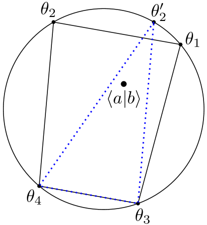
Figure 1: The point $\left\langle a|b\right\rangle$ is initially obtained as a linear combination of four points at eigenangles $\theta_{j},j=1,\dots,4$ of $U$ based on Eq. (19). A new eigenangle $\theta_{2}^{\prime}$ can be found such that $\left\langle a|b\right\rangle$ is a linear combination of $\theta_{2}^{\prime}$, $\theta_{3}$, and $\theta_{4}$.

Lemma 2.

$U$ with the minimal $\lVert U\rVert_{\vec{\mu}}$ such that Eq. (19) is satisfied can always be achieved with two non-zero eigenangles.

Proof.

Suppose the number of $\theta_{j}$ with non-zero weights (i.e., $\mbox{$\left\langle u_{j}|a\right\rangle$}\neq 0$) is $m>2$. From these $m$ vertices, pick two adjacent vertices that are either both positive or both negative. This can always be done since $m>2$. Without loss of generality (wlog), denote these two vertices as $\exp(i\theta_{1})$ and $\exp(i\theta_{2})$, and the remaining vertices as $\exp(i\theta_{3})$ to $\exp(i\theta_{m})$. Since $\sum_{j=1}^{m}\lvert\mbox{$\left\langle u_{j}|a\right\rangle$}\rvert^{2}=1$, the point $\left\langle a|b\right\rangle$ lies inside the polygon defined by the vertices $\exp(i\theta_{j}),j=1,\dots,m$, according to Eq. (19). If we replace the edge connecting $\exp(i\theta_{1})$ and $\exp(i\theta_{2})$ by their arc on the unit circle, the resultant shape will be strictly larger and contain the original polygon. This new shape can be expressed as

$$\bigcup_{\theta^{\prime}_{2}\in[\theta_{1},\theta_{2}]}\text{Polygon}(\theta^{\prime}_{2},\theta_{3},\ldots,\theta_{m})$$

where Polygon denotes the polygon defined by the vertices given in the arguments. Here, we assume $\theta_{1}\leq\theta_{2}$ wlog. Since the point $\left\langle a|b\right\rangle$ lies inside this shape, it must also lie inside one of the polygons each defined with $m-1$ vertices. Therefore, the point can be obtained as a linear combination of $m-1$ vertices (see Fig. 1). Essentially, we replace $\theta_{1}$ and $\theta_{2}$ by some $\theta^{\prime}_{2}$ defining the relevant polygon. It remains to verify that the time-energy measure using these $m-1$ vertices is no larger than before. Denote by $P(j),j=1,\ldots,{r}$, the decreasing order of $|\theta_{j}|$ where $\{\theta_{m+1},\ldots,\theta_{r}\}$ are the eigenangles of $U$ with zero weights (i.e., $\mbox{$\left\langle u_{j}|a\right\rangle$}=0$). Denote by $P^{\prime}(j),j=1,\ldots,{r}$, the decreasing order of $|\theta^{\prime}_{j}|$ where $\theta^{\prime}_{j}=\theta_{j}$ for $j=3,\ldots,m$ and $\theta^{\prime}_{j}=0$ for $j=1,m+1,\ldots,{r}$. ($\theta_{2}^{\prime}$ is defined above.) We have

$$\lVert U\rVert_{\vec{\mu}}= \sum_{j=1}^{r}\mu_{P(j)}|\theta_{j}|$$

$$\geq \sum_{j=3}^{m}\mu_{P^{\prime}(j)}|\theta^{\prime}_{j}|+\mu_{P^{\prime}(2)}\max(|\theta_{2}|,|\theta_{1}|)+$$

$$\mu_{P^{\prime}(1)}\min(|\theta_{2}|,|\theta_{1}|)+\sum_{j=m+1}^{r}\mu_{P^{\prime}(j)}|\theta_{j}|$$

$$\geq \sum_{j=3}^{m}\mu_{P^{\prime}(j)}|\theta^{\prime}_{j}|+\mu_{P^{\prime}(2)}|\theta^{\prime}_{2}|,$$

where the second last line is due to that $\sum_{j=1}^{r}\mu_{P(j)}|\theta_{j}|\geq\sum_{j=1}^{r}\mu_{P^{\prime\prime}(j)}|\theta_{j}|$ for any ordering $P^{\prime\prime}$, and the last line is due to that $\theta^{\prime}_{2}\in[\theta_{1},\theta_{2}]$. In summary, a new $U^{\prime}$ can be formed using these $m-1$ eigenangles $\{\theta^{\prime}_{2},\ldots,\theta^{\prime}_{m}\}$ with $\lVert U^{\prime}\rVert_{\vec{\mu}}\leq\lVert U\rVert_{\vec{\mu}}$. We can repeat this argument for removing another vertex until we reach $m=2$. This proves that the optimal $U$ for the time-energy measure can always be achieved with a linear combination of two vertices or, in other words, two non-zero eigenangles. ∎

This lemma implies that when finding an optimal $U$ with respect to $\lVert U\rVert_{\vec{\mu}}$, it is sufficient to consider all chords (i.e., two-vertex polygons) on the unit circle passing through the desired point $\left\langle a|b\right\rangle$. Each chord defines two eigenangles, $\theta_{1}$ and $\theta_{2}$, which in turn define a unitary transformation from $\left|a\right\rangle$ to $\left|b\right\rangle$. This transformation $\tilde{U}$ acts on the subspace spanned by $\left|a\right\rangle$ and $\left|b\right\rangle$:

$$\tilde{U} =\tilde{u}_{1}\mbox{$\left|a_{i}\right\rangle$}\mbox{$\left\langle a_{i}\right|$}+\tilde{u}_{2}\mbox{$\left|a_{i}\right\rangle$}\mbox{$\left\langle a_{i}^{\perp}\right|$}+\tilde{u}_{3}\mbox{$\left|a_{i}^{\perp}\right\rangle$}\mbox{$\left\langle a_{i}\right|$}+\tilde{u}_{4}\mbox{$\left|a_{i}^{\perp}\right\rangle$}\mbox{$\left\langle a_{i}^{\perp}\right|$}$$

$$=\begin{bmatrix}\tilde{u}_{1}&\tilde{u}_{2}\\ \tilde{u}_{3}&\tilde{u}_{4}\end{bmatrix}$$ (20)

expressed in the basis $\{\mbox{$\left|a\right\rangle$},\mbox{$\left|a^{\perp}\right\rangle$}\}$. Here,

$$\left|a^{\perp}\right\rangle =\frac{1}{\sqrt{1-\lvert\mbox{$\left\langle a|b\right\rangle$}\rvert^{2}}}\Big{(}\mbox{$\left|b\right\rangle$}-\mbox{$\left\langle a|b\right\rangle$}\mbox{$\left|a\right\rangle$}\Big{)}$$ (21)

is a vector orthogonal to $\left|a\right\rangle$ in the plane spanned by $\left|a\right\rangle$ and $\left|b\right\rangle$. (We assume $\mbox{$\left|a\right\rangle$}\neq\mbox{$\left|b\right\rangle$}$.) The entries of $\tilde{U}$ can be found by imposing that the eigenvalues are $\exp(i\theta_{1})$ and $\exp(i\theta_{2})$ and $\tilde{U}\mbox{$\left|a\right\rangle$}=\mbox{$\left|b\right\rangle$}$ (see Appendix A for detail):

$$\tilde{U}=\begin{bmatrix}\mbox{$\left\langle a|b\right\rangle$}&-e^{i(\theta_{1}+\theta_{2})}\sqrt{1-|\mbox{$\left\langle a|b\right\rangle$}|^{2}}\\ \sqrt{1-|\mbox{$\left\langle a|b\right\rangle$}|^{2}}&e^{i(\theta_{1}+\theta_{2})}\mbox{$\left\langle b|a\right\rangle$}\end{bmatrix}.$$ (22)

The overall transformation is composed of the transformation $\tilde{U}$ in the subspace spanned by $\left|a\right\rangle$ and $\left|b\right\rangle$ and a transformation $\tilde{U}^{\perp}$ in the orthogonal subspace:

$$U=\tilde{U}+\tilde{U}^{\perp}.$$ (23)

We assign $\tilde{U}^{\perp}$ with zero eigenangles:

$$\tilde{U}^{\perp}=I-\mbox{$\left|a\right\rangle$}\mbox{$\left\langle a\right|$}-\mbox{$\left|a^{\perp}\right\rangle$}\mbox{$\left\langle a^{\perp}\right|$}.$$ (24)

This ensures that $\lVert U\rVert_{\vec{\mu}}$ is minimized. Thus, $\lVert U\rVert_{\vec{\mu}}=\lVert\tilde{U}\rVert_{\vec{\mu}}=\mu_{1}|\theta_{i}|+\mu_{2}|\theta_{3-i}|$ where $i=\arg\max_{j=1,2}|\theta_{j}|$. Note that the eigenvectors corresponding to $\tilde{U}^{\perp}$ in Eq. (19) have weights $\lvert\mbox{$\left\langle u_{j}|a\right\rangle$}\rvert^{2}=0$.

IV.2 Optimal max time-energy

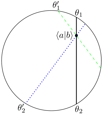
Figure 2: The optimal $U$ for the max time-energy consists of two non-trivial eigenangles $\theta_{1}$ and $\theta_{2}$ which form a vertical line passing through the point $\left\langle a|b\right\rangle$. Two other rotated lines about the point are shown. The dashed line (green) and the dotted line (blue) have max time-energy $\theta_{1}^{\prime}$ and $|\theta_{2}^{\prime}|$ respectively, which are both greater than the optimal value $\theta_{1}$.

For the max time-energy, we show that the optimal $U$ of problem (IV.1) has two non-trivial eigenangles $\theta_{1},\theta_{2}=\pm\cos^{-1}(\operatorname{Re}(\mbox{$\left\langle a|b\right\rangle$}))$, where $\cos^{-1}$ always returns an angle in the range $[0,\pi]$, and $U$ has the form of Eq. (23). The linear combination of these two eigenangles corresponds to a vertical line passing through the point $\left\langle a|b\right\rangle$ (see Fig. 2). It can easily be seen that this line gives the minimal max time-energy. Consider a line obtained by rotating the vertical line about $\left\langle a|b\right\rangle$. If $\left\langle a|b\right\rangle$ is strictly inside the unit circle, then one of the two eigenangles must become larger in magnitude, giving rise to a larger max time-energy of $\max(|\theta_{1}|,|\theta_{2}|)$. If $\left\langle a|b\right\rangle$ is on the unit circle, then one of the two eigenangles remains unchanged and so the max time-energy cannot become smaller. Therefore, we have

$$P_{\text{max}}(\mbox{$\left|a\right\rangle$},\mbox{$\left|b\right\rangle$})=f_{\text{max}}(\mbox{$\left\langle a|b\right\rangle$})=\cos^{-1}(\operatorname{Re}(\mbox{$\left\langle a|b\right\rangle$})).$$ (25)

IV.3 Sum time-energy

We only derive lower and upper bounds on the sum time-energy for problem (IV.1).

Lemma 3.

For each chord that passes through the point $r\exp(i\gamma)$, we associate a triangle formed by the origin and the chord. Among all such chords, the minimum angle of the triangle at the origin is $2\beta$ where $r=\cos(\beta)$.

Proof.

Note that the problem is invariant to the rotation by $\gamma$. Thus, wlog we assume $\gamma=0$. Let the two end points of the chord be $\exp(i\zeta_{1})$ and $\exp(-i\zeta_{2})$, where $\zeta_{1},\zeta_{2}\geq 0$. The angle in question is $\zeta_{1}+\zeta_{2}$ and we show that $\zeta_{1}+\zeta_{2}\geq 2\beta$. The point $r\exp(i0)$ is a linear combination of these two end points: $r\exp(i0)=z\exp(i\zeta_{1})+(1-z)\exp(-i\zeta_{2})$, where $0\leq z\leq 1$. Thus, $\zeta_{1}$, $\zeta_{2}$, and $z$ have to satisfy the constraint on the magnitude:

$$r^{2} =[z\cos(\zeta_{1})+(1-z)\cos(\zeta_{2})]^{2}+$$

$$\hskip 13.0pt[z\sin(\zeta_{1})-(1-z)\sin(\zeta_{2})]^{2}$$

$$=\left[2-2\cos(\zeta_{1}+\zeta_{2})\right](z^{2}-z)+1.$$

This implies that $z$ is a function of $\zeta_{1}+\zeta_{2}$. Solving the quadratic equation, we get

$$z=\frac{A\pm\sqrt{A^{2}-4A(1-r^{2})}}{2A},$$

where $A=2-2\cos(\zeta_{1}+\zeta_{2})$. Note that if $A=0$, then $\zeta_{1}=\zeta_{2}=0$ which implies that $r=1$ and $\beta=0$; thus, $0=\zeta_{1}+\zeta_{2}\geq 2\beta=0$ as claimed. Otherwise, $A>0$ and in this case, $z$ has a real solution if

$$0 \leq A-4(1-r^{2})$$

$$\Longrightarrow\cos(\zeta_{1}+\zeta_{2}) \leq 2r^{2}-1=2\cos^{2}(\beta)-1=\cos(2\beta)$$

where $r=\cos(\beta)$. Since $\cos$ is a decreasing function in the domain $[0,\pi]$, $\zeta_{1}+\zeta_{2}\geq 2\beta$ as claimed. ∎

Remark 2.

Note that the minimum angle of $2\beta$ in Lemma 3 is achieved by the triangle formed by the origin and the chord perpendicular to the line connecting the origin and $r\exp(i\gamma)$.

Lemma 4.

The solution to problem (IV.1) for the sum time-energy is lower bounded as follows:

$$P_{\text{{\rm sum}}}(\mbox{$\left|a\right\rangle$},\mbox{$\left|b\right\rangle$})=f_{\text{{\rm sum}}}(\mbox{$\left\langle a|b\right\rangle$})\geq \>2\cos^{-1}|\mbox{$\left\langle a|b\right\rangle$}|$$

$$\equiv \>f_{\text{{\rm sum}}}^{\text{L}}(\mbox{$\left\langle a|b\right\rangle$}).$$ (26)

Proof.

The sum time-energy of $U$ is $|\theta_{1}|+|\theta_{2}|$ since $U$ has only two non-trivial eigenangles due to Lemma 2. The chord defined by these two eigenangles, $\theta_{1}$ and $\theta_{2}$, passes through the point $\mbox{$\left\langle a|b\right\rangle$}=r\exp(i\gamma)$, where $r=|\mbox{$\left\langle a|b\right\rangle$}|$. We consider the triangle formed by the origin and the chord and focus on the angle at the origin. For the case $\theta_{1}>0$, $\theta_{2}\leq 0$ and the case $\theta_{1}\leq 0$, $\theta_{2}>0$, this angle is $\min(|\theta_{1}-\theta_{2}|,2\pi-|\theta_{1}-\theta_{2}|)$. According to Lemma 3, this angle is lower bounded by $2\beta$ where $\beta=\cos^{-1}(r)$. Thus,

$$|\theta_{1}|+|\theta_{2}|=|\theta_{1}-\theta_{2}| \geq\min(|\theta_{1}-\theta_{2}|,2\pi-|\theta_{1}-\theta_{2}|)$$

$$\geq 2\beta.$$

Equality is achieved when $|\theta_{1}-\theta_{2}|\leq\pi$ and the chord described by $\theta_{1}$ and $\theta_{2}$ is perpendicular to the line connecting the origin and $r\exp(i\gamma)$ (see Remark 2). For the case $\theta_{1},\theta_{2}>0$, the case $\theta_{1},\theta_{2}<0$, and the case $\theta_{1}=\theta_{2}=0$, the angle is $|\theta_{1}-\theta_{2}|$ which is lower bounded by $2\beta$ according to Lemma 3. Thus, we have

$$|\theta_{1}|+|\theta_{2}|\geq|\theta_{1}-\theta_{2}|\geq 2\beta.$$

∎

Lemma 5.

The solution to problem (IV.1) for the sum time-energy is upper bounded as follows:

$$P_{\text{{\rm sum}}}(\mbox{$\left|a\right\rangle$},\mbox{$\left|b\right\rangle$})=f_{\text{{\rm sum}}}(\mbox{$\left\langle a|b\right\rangle$})\leq \>2\cos^{-1}(\operatorname{Re}(\mbox{$\left\langle a|b\right\rangle$}))$$

$$\equiv \>f_{\text{{\rm sum}}}^{\text{U}}(\mbox{$\left\langle a|b\right\rangle$}).$$ (27)

Proof.

Any $U$ that satisfies $U\mbox{$\left|a\right\rangle$}=\mbox{$\left|b\right\rangle$}$ (i.e., the constraint of problem (IV.1)) serves as an upper bound to $P_{\vec{\mu}}(\mbox{$\left|a\right\rangle$},\mbox{$\left|b\right\rangle$})$ for any $\vec{\mu}$. Thus, for simplicity, we choose the optimal $U$ that achieves the optimal max time-energy in Eq. (25) to serve as an upper bound to $P_{\text{sum}}(\mbox{$\left|a\right\rangle$},\mbox{$\left|b\right\rangle$})$. This $U$ has two non-trivial eigenangles $\theta_{1}=\cos^{-1}(\operatorname{Re}(\mbox{$\left\langle a|b\right\rangle$}))$ and $\theta_{2}=-\theta_{1}$. Thus, the sum time-energy of this $U$ is $|\theta_{1}|+|\theta_{2}|=2\cos^{-1}(\operatorname{Re}(\mbox{$\left\langle a|b\right\rangle$}))$, and this is an upper bound to $P_{\text{sum}}(\mbox{$\left|a\right\rangle$},\mbox{$\left|b\right\rangle$})$. ∎

V Time-energy upper bound

In this section, we consider upper bounding $\lVert\mathcal{F}\rVert_{\vec{\mu}}$ given its Kraus operators $(F_{1},F_{2},\dots,F_{{d}})$ by upper bounding $\lVert g(F_{1:{d}})\rVert_{\vec{\mu}}$. Any implementation $U$ of the quantum channel $\mathcal{F}$ serves as an upper bound to $\lVert\mathcal{F}\rVert_{\vec{\mu}}$ since $\lVert\mathcal{F}\rVert_{\vec{\mu}}\leq\lVert U\rVert_{\vec{\mu}}$ for all $U$ of the form of Eq. (12). We propose a simple method to construct a time-energy efficient $U$ that completes the partial matrix $g(F_{1:{d}})$, and $\lVert U\rVert_{\vec{\mu}}$ will serve as an upper bound to the “partial $U$ problem” (II.2) for $\lVert g(F_{1:{d}})\rVert_{\vec{\mu}}$, which is an intermediate problem to the ultimate “channel problem” (II.2).

V.1 Successive construction of $U$

We focus on finding an upper bound to the “partial $U$ problem” (II.2) which was recast as problem (III) which finds a unitary matrix $U$ that satisfies $n$ transformation rules: $\mbox{$\left|e_{i}\right\rangle$}\longrightarrow\mbox{$\left|b_{i}\right\rangle$}\>\>\text{for all }i=1,\ldots,n$. Here, we focus on the “partial $U$ problem” for $\lVert g(F_{1:{d}})\rVert_{\vec{\mu}}$. Thus, $\left|b_{i}\right\rangle$ is the $i$th column of $g(F_{1:{d}})$. In Sec. IV, we analyzed the optimal unitary operation $U_{i}$ for each single-vector transformation $\mbox{$\left|e_{i}\right\rangle$}\longrightarrow\mbox{$\left|b_{i}\right\rangle$}$, and we solved $\lVert U_{i}\rVert_{\text{max}}$ and bounded $\lVert U_{i}\rVert_{\text{sum}}$. Motivated by this result, we propose a greedy method to construct $U$ in which we successively construct the best unitary $U_{i}$ for each $i=1,\ldots,n$, and concatenate them. The overall $U$ will be

$$U=U_{n}\dots U_{1}.$$ (28)

We design each $U_{i}$ as follows. When we consider the first transformation (i.e., $i=1$), we seek the optimal $U_{1}$ with the minimal $\lVert U_{1}\rVert_{\vec{\mu}}$ such that

$$U_{1}\mbox{$\left|e_{1}\right\rangle$}=\mbox{$\left|b_{1}\right\rangle$}.$$

When $i=2$, we seek the optimal $U_{2}$ such that

$$U_{2}U_{1}\mbox{$\left|e_{2}\right\rangle$}=\mbox{$\left|b_{2}\right\rangle$}.$$

In general, for the $i$th transformation, we seek the optimal $U_{i}$ such that

$$U_{i}\mbox{$\left|a_{i}\right\rangle$}=\mbox{$\left|b_{i}\right\rangle$}$$ (29)

where

$$\mbox{$\left|a_{i}\right\rangle$}=U_{i-1}\cdots U_{1}\mbox{$\left|e_{i}\right\rangle$}\text{ for }n\geq i\geq 2\text{ and }\mbox{$\left|a_{1}\right\rangle$}=\mbox{$\left|e_{1}\right\rangle$}.$$ (30)

Note that the optimal $U_{i}$ with the minimal $\lVert U_{i}\rVert_{\vec{\mu}}$ has already been considered in problem (IV.1). We obtained the optimal value for $\lVert U_{i}\rVert_{\text{max}}$ and lower and upper bounds for $\lVert U_{i}\rVert_{\text{sum}}$ (see Eqs. (25), (26), (27) ). Thus,

$$\lVert U_{i}\rVert_{\vec{\mu}}=f_{\vec{\mu}}(\mbox{$\left\langle a_{i}|b_{i}\right\rangle$})$$ (31)

where the RHS comes from Eq. (18).

A key feature of our construction is that we design $U_{i}$’s successively in a backward-looking fashion; i.e., when we design $U_{i}$, we only need to know $U_{j}$ for $j<i$ and we do not use $U_{j}$ for $j>i$.

In order for this successive approach to work, the action of a higher-index $U_{j}$ should not affect the transformation of a lower index $i<j$, i.e.,

$$U_{i+1}U_{i}\mbox{$\left|a_{i}\right\rangle$} =\mbox{$\left|b_{i}\right\rangle$}$$

$$U_{i+2}U_{i+1}U_{i}\mbox{$\left|a_{i}\right\rangle$} =\mbox{$\left|b_{i}\right\rangle$}$$

$$\vdots$$

$$U_{n}\cdots U_{i+2}U_{i+1}U_{i}\mbox{$\left|a_{i}\right\rangle$} =\mbox{$\left|b_{i}\right\rangle$}.$$ (32)

Only if the last equation holds for all $i$ does the overall $U$ transforms according to Eq. (15) as required. We show that Eq. (32) does hold.

Lemma 6.

(Backward-looking design of $U_{i}$)

$$U_{i+j}\cdots U_{i+2}U_{i+1}U_{i}\mbox{$\left|a_{i}\right\rangle$} =\mbox{$\left|b_{i}\right\rangle$}$$ (33)

for $j\geq 1$ when Eq. (29) holds.

Proof.

We need to use the essential properties that $\mbox{$\left\langle e_{i}|e_{k}\right\rangle$}=\mbox{$\left\langle b_{i}|b_{k}\right\rangle$}=\delta_{ik}$ where $\delta_{ik}$ is the Kronecker delta. We prove by induction. First we compute $U_{i+1}U_{i}\mbox{$\left|a_{i}\right\rangle$}$. Recall from Eq. (23) that $U_{i+1}$ performs a non-trivial transformation only in the subspace spanned by $\left|a_{i+1}\right\rangle$ and $\left|b_{i+1}\right\rangle$. We show that $U_{i}\mbox{$\left|a_{i}\right\rangle$}$ is not in this subspace. Note that

$$\mbox{$\left\langle a_{i+1}\right|$}{U_{i}\mbox{$\left|a_{i}\right\rangle$}} =\left[\mbox{$\left\langle e_{i+1}\right|$}U_{1}^{\dagger}U_{2}^{\dagger}\cdots U_{i}^{\dagger}\right]U_{i}\Big{[}U_{i-1}\cdots U_{1}\mbox{$\left|e_{i}\right\rangle$}\Big{]}$$ (34)

$$=0$$

by Eq. (30), and also $\mbox{$\left\langle b_{i+1}\right|$}{U_{i}\mbox{$\left|a_{i}\right\rangle$}}=\mbox{$\left\langle b_{i+1}|b_{i}\right\rangle$}=0$ by Eq. (29). Hence, $U_{i}\mbox{$\left|a_{i}\right\rangle$}$ is not in the aforementioned subspace. This shows that

$$U_{i+1}U_{i}\mbox{$\left|a_{i}\right\rangle$} =(\tilde{U}_{i+1}+\tilde{U}_{i+1}^{\perp})U_{i}\mbox{$\left|a_{i}\right\rangle$}$$

$$=\tilde{U}_{i+1}^{\perp}U_{i}\mbox{$\left|a_{i}\right\rangle$}$$

$$=U_{i}\mbox{$\left|a_{i}\right\rangle$}$$

$$=\mbox{$\left|b_{i}\right\rangle$}$$

since $\tilde{U}_{i+1}^{\perp}$ acts trivially on the orthogonal complement of the subspace spanned by $\left|a_{i+1}\right\rangle$ and $\left|b_{i+1}\right\rangle$ (c.f. Eq. (24)).

Now consider $U_{i+j}\cdots U_{i+1}U_{i}\mbox{$\left|a_{i}\right\rangle$}$ assuming the hypothesis $U_{i+j-1}\cdots U_{i+1}U_{i}\mbox{$\left|a_{i}\right\rangle$}=\mbox{$\left|b_{i}\right\rangle$}$. Similar to Eq. (34),

$$\mbox{$\left\langle a_{i+j}\right|$}{U_{i+j-1}\cdots U_{i+1}U_{i}\mbox{$\left|a_{i}\right\rangle$}}$$

$$= \left[\mbox{$\left\langle e_{i+j}\right|$}U_{1}^{\dagger}U_{2}^{\dagger}\cdots U_{i+j-1}^{\dagger}\right]U_{i+j-1}\cdots$$

$$U_{i+1}U_{i}\Big{[}U_{i-1}\dots U_{1}\mbox{$\left|e_{i}\right\rangle$}\Big{]}$$

$$= 0$$

and

$$\mbox{$\left\langle b_{i+j}\right|$}{U_{i+j-1}\cdots U_{i+1}U_{i}\mbox{$\left|a_{i}\right\rangle$}}=\mbox{$\left\langle b_{i+j}|b_{i}\right\rangle$}=0$$

using the hypothesis.

Therefore, ${U_{i+j-1}\cdots U_{i+1}U_{i}\mbox{$\left|a_{i}\right\rangle$}}$ is not in the subspace spanned by $\left|a_{i+j}\right\rangle$ and $\left|b_{i+j}\right\rangle$ (the subspace that $U_{i+j}$ acts non-trivially), and thus

$$U_{i+j}U_{i+j-1}\cdots U_{i+1}U_{i}\mbox{$\left|a_{i}\right\rangle$}=U_{i+j-1}\cdots U_{i+1}U_{i}\mbox{$\left|a_{i}\right\rangle$}=\mbox{$\left|b_{i}\right\rangle$}.$$

This proves the claim. ∎

This is the key lemma that allows us to compute an upper bound in a successive manner. In essence, instead of considering the original problem of finding a unitary required to perform $n$ simultaneous transformations, we consider the problem of finding $n$ unitaries each required to perform one transformation. Note that we already solved the latter problem in Sec. IV.1. In particular, the max time-energy for a single-vector transformation is given in Eq. (25). Thus, according to Eq. (28),

$$\lVert U\rVert_{\vec{\mu}} =\lVert U_{n}\dots U_{1}\rVert_{\vec{\mu}}$$

$$\leq\sum_{i=1}^{n}\lVert U_{i}\rVert_{\vec{\mu}}$$

$$=\sum_{i=1}^{n}f_{\vec{\mu}}(\mbox{$\left\langle a_{i}|b_{i}\right\rangle$})$$ (35)

where the inequality is due to the triangle inequality of the norm $\lVert\cdot\rVert_{\vec{\mu}}$ (see Theorem 2 of Ref. Chau (2011)) and the last line is due to Eq. (31).

In light of Remark 1, we can always assume that $F_{1}$ is initially given in upper triangular form. In the following, we use this property to further deduce a simple bound on $\lVert U\rVert_{\vec{\mu}}$ and consequently $\lVert\mathcal{F}\rVert_{\vec{\mu}}$. We show that when $F_{1}$ is upper triangular (which can always be guaranteed by Remark 1), $\mbox{$\left|a_{i}\right\rangle$}=\mbox{$\left|e_{i}\right\rangle$}$ for all $1\leq i\leq n$ in Eqs. (29)–(30). Thus, $\lVert U_{i}\rVert_{\vec{\mu}}$ in Eq. (35) will only depend on $\left\langle e_{i}|b_{i}\right\rangle$ which is the $i$th eigenvalue of $F_{1}$.

Lemma 7.

(Independent design of $U_{i}$) When $F_{1}$ is upper triangular, $\mbox{$\left|a_{i}\right\rangle$}=\mbox{$\left|e_{i}\right\rangle$}$ for all $1\leq i\leq n$ in Eqs. (29)–(30), which implies that designing according to

$$U_{i}\mbox{$\left|e_{i}\right\rangle$}=\mbox{$\left|b_{i}\right\rangle$}$$ (36)

and designing according to Eq. (29) are equivalent.

Proof.

Note that since $F_{1}$ is upper triangular, $\mbox{$\left\langle b_{j}|e_{i}\right\rangle$}=0$ for $j<i\leq n$. We prove by induction. We show that $\mbox{$\left|a_{i}\right\rangle$}=\mbox{$\left|e_{i}\right\rangle$}$ assuming the hypothesis that $\mbox{$\left|a_{j}\right\rangle$}=\mbox{$\left|e_{j}\right\rangle$}$ for $j<i$ is true. Note that $\mbox{$\left|a_{1}\right\rangle$}=\mbox{$\left|e_{1}\right\rangle$}$ by definition in Eq. (30). Recall from Eq. (23) that $U_{j}$ performs a non-trivial transformation only in the subspace spanned by $\left|a_{j}\right\rangle$ and $\left|b_{j}\right\rangle$. We show that $\left|e_{i}\right\rangle$ for $i>j$ is not in this subspace: $\mbox{$\left\langle a_{j}|e_{i}\right\rangle$}=\mbox{$\left\langle e_{j}|e_{i}\right\rangle$}=0$ where we assume that the hypothesis is true, and $\mbox{$\left\langle b_{j}|e_{i}\right\rangle$}=0$ due to the triangular structure of $F_{1}$. This means that for $i>j$,

$$U_{j}\mbox{$\left|e_{i}\right\rangle$} =(\tilde{U}_{j}+\tilde{U}_{j}^{\perp})\mbox{$\left|e_{i}\right\rangle$}$$

$$=\tilde{U}_{j}^{\perp}\mbox{$\left|e_{i}\right\rangle$}$$

$$=\mbox{$\left|e_{i}\right\rangle$}$$

since $\tilde{U}_{j}^{\perp}$ acts trivially (c.f. Eq. (24)). This shows that

$$\left|a_{i}\right\rangle =U_{i-1}\cdots U_{1}\mbox{$\left|e_{i}\right\rangle$}$$

$$=\mbox{$\left|e_{i}\right\rangle$}.$$

∎

This lemma allows us to compute the upper bound easier since the upper bound in Eq. (35) now becomes

$$\lVert U\rVert_{\vec{\mu}} \leq\sum_{i=1}^{n}f_{\vec{\mu}}(\mbox{$\left\langle e_{i}|b_{i}\right\rangle$})$$ (37)

$$=\sum_{i=1}^{n}f_{\vec{\mu}}(\lambda_{i}(F_{1}))$$ (38)

where we recognize that the diagonal elements of $F_{1}$ are its eigenvalues, denoted by $\lambda_{i}(F_{1})$. This shows that $\lVert U\rVert_{\vec{\mu}}$ only depends on the eigenvalues of one Kraus operator of the quantum channel. Since $\lVert\mathcal{F}\rVert_{\vec{\mu}}\leq\lVert U\rVert_{\vec{\mu}}$ for all $U$ of the form of Eq. (12), we have

$$\halign to=0.0pt{ \hfil$\displaystyle{#}$&\hfil$\displaystyle{{}#{}}$\hfil&\hfil$\displaystyle{{}#{}}$\hfil&$\displaystyle{#}$\hfil&\refstepcounter{equation}\label{#}\llap{(\theequation)}\cr\vskip-6.0pt\cr\lVert\mathcal{F} \rVert_{\vec{\mu}} &\leq&\min_{\mathbf{v}} &\sum_{i=1}^{n} f_{\vec{\mu}}(\lambda_{i}(\sum_{j=1}^{d} v_{j} F_{j}))\cr&&\text{s.t.}&\sum_{j=1}^{d} |v_{j}|^{2} \leq 1 .&\hbox to0.0pt{\hss(39\cr}}$$

Here, $\mathbf{v}$ corresponds to the first $d$ elements of the first row of $W_{B}$ in Eq. (12). This bound holds for any quantum channel $\mathcal{F}$ described by Kraus operators $F_{i},i=1,\dots,d$.

V.2 Max time-energy upper bound

For the max time-energy, we substitute $f_{\text{max}}$ in Eq. (25) for $f_{\vec{\mu}}$ in Eq. (V.1) to get

$$\lVert\mathcal{F}\rVert_{\text{max}} \leq\min_{\mathbf{v}:\>\lVert\mathbf{v}\rVert\leq 1}\sum_{i=1}^{n}\cos^{-1}\Big{[}\operatorname{Re}(\lambda_{i}(\sum_{j=1}^{d}v_{j}F_{j}))\Big{]}.$$ (40)

V.3 Sum time-energy upper bound

For the sum time-energy, we substitute $f_{\text{sum}}^{\text{U}}$ in Eq. (27) for $f_{\vec{\mu}}$ in Eq. (V.1) to get

$$\lVert\mathcal{F}\rVert_{\text{sum}} \leq\min_{\mathbf{v}:\>\lVert\mathbf{v}\rVert\leq 1}\sum_{i=1}^{n}2\cos^{-1}\Big{[}\operatorname{Re}(\lambda_{i}(\sum_{j=1}^{d}v_{j}F_{j}))\Big{]}.$$ (41)

V.4 Special case: diagonal $F_{1}$

Here, we consider the special class of channels for which $F_{1}$ is diagonal, which will be useful for showing the optimal time-energy for a class of channels in Sec. VII. Following the construction of $U$ in Eq. (28), we argue not only that we can independently design $U_{i}$ (Lemma 7), but also that they act on orthogonal subspaces (meaning that they commute). According to Lemma 7, $U_{i}$ transforms $\left|e_{i}\right\rangle$ to $\left|b_{i}\right\rangle$, and is the solution to problem (IV.1) where $\mbox{$\left|a\right\rangle$}=\mbox{$\left|e_{i}\right\rangle$}$ and $\mbox{$\left|b\right\rangle$}=\mbox{$\left|b_{i}\right\rangle$}$. Thus, its non-trivial part $\tilde{U}_{i}$ [see Eq. (23)] acts on the subspace spanned by $\{\mbox{$\left|e_{i}\right\rangle$},\mbox{$\left|b_{i}\right\rangle$}\}$.

The fact that $F_{1}$ is diagonal gives rise to the following property: $\mbox{$\left\langle e_{i}|b_{j}\right\rangle$}=0$ if $i\neq j$ where $1\leq i,j\leq n$. Also, we already have $\mbox{$\left\langle e_{i}|e_{j}\right\rangle$}=0$ if $i\neq j$ by definition and $\mbox{$\left\langle b_{i}|b_{j}\right\rangle$}=0$ if $i\neq j$ by the trace-preserving property of quantum channels. Thus, the subspaces spanned by $\{\mbox{$\left|e_{i}\right\rangle$},\mbox{$\left|b_{i}\right\rangle$}\}$ for $i=1,\dots,n$ are orthogonal to each other. This means that $\tilde{U}_{i}$ acting on these subspaces [see Eq. (20)] are orthogonal to each other. Then we may bypass the construction of $U_{i}$ in Eq. (23) and directly form

$$U=\sum_{i=1}^{n}\tilde{U}_{i}+P_{U^{\perp}}$$

where $P_{U^{\perp}}$ is the projection onto the subspace orthogonal to the summation term. Thus, the set of non-zero eigenangles of $U$ is composed of the eigenangles of $\tilde{U}_{i}$ for all $i=1,\dots,n$. This means that

$$\lVert U\rVert_{\text{max}} =\max_{1\leq i\leq n}\lVert\tilde{U}_{i}\rVert_{\text{max}}$$ (42)

$$\lVert U\rVert_{\text{sum}} =\sum_{i=1}^{n}\lVert\tilde{U}_{i}\rVert_{\text{sum}}.$$ (43)

Thus, for this class of channels, by using Eqs. (25), (27), (31) and $\lVert U_{i}\rVert_{\vec{\mu}}=\lVert\tilde{U}_{i}\rVert_{\vec{\mu}}$, we have

$$\lVert\mathcal{F}\rVert_{\text{max}} \leq\lVert U\rVert_{\text{max}}=\max_{1\leq i\leq n}\cos^{-1}[\operatorname{Re}(\lambda_{i}(F_{1}))]$$ (44)

$$\lVert\mathcal{F}\rVert_{\text{sum}} \leq\lVert U\rVert_{\text{sum}}\leq\sum_{i=1}^{n}2\cos^{-1}[\operatorname{Re}(\lambda_{i}(F_{1}))].$$ (45)

VI Time-energy Lower bound

VI.1 General form of lower bound

We lower bound $\lVert\mathcal{F}\rVert_{\vec{\mu}}$ of the “channel problem” (II.2). We first consider lower bounding $\lVert g(F_{1:{d}})\rVert_{\vec{\mu}}$ for a fixed set of Kraus operators $(F_{1},F_{2},\dots,F_{{d}})$. Note that $\lVert g(F_{1:{d}})\rVert_{\vec{\mu}}$ is obtained from the “partial $U$ problem” (III), and we propose a modified problem whose solution lower bounds this problem. The modified problem is formed by removing all except one transformation constraints in problem (III) as follows:

$$\halign to=0.0pt{ \hfil$\displaystyle{#}$&\hfil$\displaystyle{{}#{}}$\hfil&\hfil$\displaystyle{{}#{}}$\hfil&$\displaystyle{#}$\hfil&\refstepcounter{equation}\label{#}\llap{(\theequation)}\cr\vskip-6.0pt\cr P_{\vec{\mu}}(\mbox{$\left|e_{i}\right\rangle$},\mbox{$\left|b_{i}\right\rangle$}) &=&\displaystyle\min_{U} &\lVert U \rVert_{\vec{\mu}}\cr&&\text{s.t.}&U\mbox{$\left|e_{i}\right\rangle$} = \mbox{$\left|b_{i}\right\rangle$}\text{ with}\cr&&&U \in\operatorname{U}(r) \crcr}$$

which is defined for $i=1,\dots,n$. Here $\left|b_{i}\right\rangle$ is the $i$th column of $g(QF_{1}Q^{\dagger},F_{2}Q^{\dagger},\dots,F_{{d}}Q^{\dagger})$ where $QF_{1}Q^{\dagger}$ is an upper triangular matrix corresponding to the Schur decomposition of $F_{1}$ (see Remark 1). Note that this problem is the single-vector problem (IV.1) which we analyzed in Sec. IV. Certainly, the feasible set of this problem contains that of problem (III), and so with the help of Lemma 1, we have $\lVert g(F_{1},F_{2},\dots,F_{{d}})\rVert_{\vec{\mu}}=\lVert g(QF_{1}Q^{\dagger},F_{2}Q^{\dagger},\dots,F_{{d}}Q^{\dagger})\rVert_{\vec{\mu}}\geq P_{\vec{\mu}}(\mbox{$\left|e_{i}\right\rangle$},\mbox{$\left|b_{i}\right\rangle$})$ for all $i=1,\dots,n$. Thus,

$$\lVert g(F_{1},F_{2},\dots,F_{{d}})\rVert_{\vec{\mu}} \geq\max_{1\leq i\leq n}P_{\vec{\mu}}(\mbox{$\left|e_{i}\right\rangle$},\mbox{$\left|b_{i}\right\rangle$})$$

$$=\max_{1\leq i\leq n}f_{\vec{\mu}}(\mbox{$\left\langle e_{i}|b_{i}\right\rangle$})$$

$$=\max_{1\leq i\leq n}f_{\vec{\mu}}(\lambda_{i}(F_{1}))$$

where we used Eq. (18) in the second line and the third line is due to Remark 1 with $\lambda_{i}(F_{1})$ being the $i$th eigenvalue of $F_{1}$. Note that the last inequality holds when the LHS is replaced by $\lVert g(F_{1},F_{2},\dots,F_{{d}},\mathbf{0},\dots,\mathbf{0})\rVert_{\vec{\mu}}$ for any number of extra all-zero Kraus operators inserted. Combining with the “channel problem” (II.2) , we have

$$\halign to=0.0pt{ \hfil$\displaystyle{#}$&\hfil$\displaystyle{{}#{}}$\hfil&\hfil$\displaystyle{{}#{}}$\hfil&$\displaystyle{#}$\hfil&\refstepcounter{equation}\label{#}\llap{(\theequation)}\cr\vskip-6.0pt\cr\lVert\mathcal{F} \rVert_{\vec{\mu}} &\geq&\min_{\mathbf{v}} &\max_{1\leq i \leq n} f_{\vec{\mu}}(\lambda_{i}(\sum_{j=1}^{d} v_{j} F_{j}))\cr&&\text{s.t.}&\sum_{j=1}^{d} |v_{j}|^{2} \leq 1 .&\hbox to0.0pt{\hss(46\cr}}$$

Here, $\mathbf{v}$ corresponds to the first $d$ elements of the first row of $W_{B}$ in Eq. (12). This bound holds for any quantum channel $\mathcal{F}$ described by Kraus operators $F_{i},i=1,\dots,d$.

VI.2 Max time-energy lower bound

For the max time-energy, we substitute $f_{\text{max}}$ in Eq. (25) for $f_{\vec{\mu}}$ in Eq. (VI.1) to get

$$\lVert\mathcal{F}\rVert_{\text{max}}\geq \min_{\mathbf{v}:\>\lVert\mathbf{v}\rVert\leq 1}\>\>\max_{1\leq i\leq n}\cos^{-1}\Big{[}\operatorname{Re}(\lambda_{i}(\sum_{j=1}^{d}v_{j}F_{j}))\Big{]}.$$ (47)

VI.3 Sum time-energy lower bound

For the sum time-energy, we substitute $f_{\text{sum}}$ for $f_{\vec{\mu}}$ in Eq. (VI.1) to get

$$\lVert\mathcal{F}\rVert_{\text{sum}}\geq\min_{\mathbf{v}:\>\lVert\mathbf{v}\rVert\leq 1}\>\>\max_{1\leq i\leq n}f_{\text{sum}}(\lambda_{i}(\sum_{j=1}^{d}v_{j}F_{j}))$$ (48)

and it is a simple argument to argue that the lower bound of $\lVert\mathcal{F}\rVert_{\text{sum}}$ can be given in terms of $f_{\text{sum}}^{\text{L}}$ defined in Eq. (26). First, note that

$$P(\mathbf{v}) \equiv\max_{i}f_{\text{sum}}(\lambda_{i}(\sum_{j=1}^{d}v_{j}F_{j}))$$

$$\geq\max_{i}f_{\text{sum}}^{\text{L}}(\lambda_{i}(\sum_{j=1}^{d}v_{j}F_{j}))\equiv Q(\mathbf{v})$$

for all $\mathbf{v}$. And we have

$$\min_{\mathbf{v}}P(\mathbf{v})=P(\mathbf{\hat{v}})\geq Q(\mathbf{\hat{v}})\geq\min_{\mathbf{v}}Q(\mathbf{v})$$

where $\mathbf{\hat{v}}=\arg\min_{\mathbf{v}}P(\mathbf{v})$. Therefore, we have

$$\lVert\mathcal{F}\rVert_{\text{sum}} \geq\min_{\mathbf{v}:\>\lVert\mathbf{v}\rVert\leq 1}Q(\mathbf{v})$$

$$=\min_{\mathbf{v}:\>\lVert\mathbf{v}\rVert\leq 1}\>\>\max_{1\leq i\leq n}2\cos^{-1}|\lambda_{i}(\sum_{j=1}^{d}v_{j}F_{j})|.$$

Note that $Q(\mathbf{v})\leq Q(\kappa\mathbf{v})$ for $0\leq\kappa\leq 1$, and thus we have

$$\lVert\mathcal{F}\rVert_{\text{sum}} \geq\min_{\mathbf{v}:\>\lVert\mathbf{v}\rVert=1}\>\>\max_{1\leq i\leq n}2\cos^{-1}|\lambda_{i}(\sum_{j=1}^{d}v_{j}F_{j})|.$$ (49)

VII Optimal time-energy for a class of channels

Definition 1.

Define a class $\mathcal{C}(n)$ of quantum channels acting on $n\times n$ density matrices where each channel is described by Kraus operators $\{F_{j}\in{\mathbb{C}}^{n\times n}:j=1,\ldots,d\}$ of the form

$${F}_{1} =\sqrt{p}I\text{ where $0\leq p\leq 1$}$$ (50)

$${\rm Tr}({F}_{j}) =0,\>\>j=2,\ldots,d.$$

The number $d$ of Kraus operators of each channel can be different.

Note that this class contains the depolarizing channel, the bit-flip channel, and the phase-flip channel.

VII.1 Optimal max time-energy

We show that the lower bound of $\lVert\mathcal{F}\rVert_{\text{max}}$ in Eq. (47) is achievable for any $\mathcal{F}\in\mathcal{C}(n)$ with $2\leq n<\infty$. The RHS of Eq. (47) can be written as

$$\cos^{-1}\Big{[}\max_{\mathbf{v}:\>\lVert\mathbf{v}\rVert\leq 1}\>\>\min_{1\leq i\leq n}\operatorname{Re}(\lambda_{i}(\sum_{j=1}^{d}v_{j}F_{j}))\Big{]},$$ (51)

since $\cos^{-1}$ is a decreasing function in the range $[0,\pi]$. Consider part of this term:

$$P(\mathbf{v}) \equiv\min_{1\leq i\leq n}\operatorname{Re}(\lambda_{i}(\sum_{j=1}^{d}v_{j}F_{j}))$$

$$\leq\frac{1}{n}\sum_{i=1}^{n}\operatorname{Re}(\lambda_{i}(\sum_{j=1}^{d}v_{j}F_{j}))\equiv Q(\mathbf{v}).$$

Let the eigenvalues of $\sum_{j=2}^{d}v_{j}F_{j}$ be $\{\sigma_{1},\dots,\sigma_{n}\}$. Note that $\sum_{i=1}^{n}\sigma_{i}=0$. Thus,

$$\lambda_{i}(\sum_{j=1}^{d}v_{j}F_{j})=v_{1}\sqrt{p}+\sigma_{i}$$

and

$$Q(\mathbf{v})=\frac{1}{n}\sum_{i=1}^{n}\operatorname{Re}(v_{1}\sqrt{p}+\sigma_{i})=\operatorname{Re}(v_{1}\sqrt{p})\leq\sqrt{p}.$$

Considering the maximization in Eq. (51),

$$\max_{\mathbf{v}}P(\mathbf{v})\leq Q(\mathbf{\hat{v}})\leq\max_{\mathbf{v}}Q(\mathbf{v})$$

where $\mathbf{\hat{v}}$ is the optimal value of the maximization of $P$. Thus,

$$\lVert\mathcal{F}\rVert_{\text{max}}\geq\cos^{-1}(\max_{\mathbf{v}}P(\mathbf{v}))\geq\cos^{-1}(\sqrt{p})$$

since $\cos^{-1}$ is a decreasing function in the range $[0,\pi]$. Note that the RHS coincides with the upper bound from Eq. (44) where $\lambda_{i}(F_{1})=\sqrt{p}$. Therefore,

$$\lVert\mathcal{F}\rVert_{\text{max}}=\cos^{-1}(\sqrt{p})$$ (52)

for any $\mathcal{F}\in\mathcal{C}(n)$ with $2\leq n<\infty$.

VIII Some interesting consequences

VIII.1 Comparison of quantum and classical noisy channels

The quantum noisy channel or the quantum depolarizing channel acting on $n\times n$ density matrices is defined as

$$\mathcal{F}_{Q}(\rho) \triangleq q\rho+(1-q)\frac{I}{n}$$

where complete positivity requires that $-1/(n^{2}-1)\leq q\leq 1$ King (2003).

The Weyl operators are the $n$-dimensional generalization of the Pauli operators and are defined as

$$S_{jk}=\sum_{s=0}^{n-1}\omega^{sk}\mbox{$\left|s+j\right\rangle$}\mbox{$\left\langle s\right|$}\in{\mathbb{C}}^{n\times n}$$

where $j,k=0,\dots,n-1$ and $\omega$ is the $n$th root of unity. These operators have the following properties:

• (Identity) $S_{00}=I$.

• (Traceless) ${\rm Tr}(S_{jk})=0$ for $(j,k)\neq(0,0)$.

• (Complete erasure) $n^{-2}\sum_{j,k=0}^{n-1}S_{jk}\rho S_{jk}^{\dagger}=n^{-1}I$ for any density matrix $\rho$.

• (Trace preserving) $n^{-2}\sum_{j,k=0}^{n-1}S_{jk}^{\dagger}S_{jk}=I$.

• (Complete erasure) $n^{-1}\sum_{j=0}^{n-1}S_{j0}\rho S_{j0}^{\dagger}=n^{-1}I$ for any diagonal density matrix $\rho$.

• (Trace preserving) $n^{-1}\sum_{j}^{n-1}S_{j0}^{\dagger}S_{j0}=I$.

We may express the quantum noisy channel using the Weyl’s operators:

$$\mathcal{F}_{Q}(\rho) =qI\rho I+(1-q)\frac{1}{n^{2}}\sum_{j,k=0}^{n-1}S_{jk}\rho S_{jk}^{\dagger}.$$ (53)

The advantage of doing so is that we can now see that $\mathcal{F}_{Q}(\rho)$ is in the class $\mathcal{C}(n)$ (defined in Definition 1) and we can apply Eq. (52) to get the max time-energy of it.

In a similar manner, we define the classical noisy channel which adds classical noise (i.e., classical states are being remapped):

$$\mathcal{F}_{C}(\rho) \triangleq qI\rho I+(1-q)\frac{1}{n}\sum_{j=0}^{n-1}S_{j0}\rho S_{j0}^{\dagger},$$ (54)

where $-1/(n-1)\leq q\leq 1$ for complete positivity. When $\rho$ is diagonal (i.e., a mixture of classical states),

$$\mathcal{E}_{C}(\rho)=q\rho+(1-q)\frac{I}{n}.$$

We now verify that we have a fair comparison between the quantum and classical noisy channels, by checking that the same amount of noise is added to the input states of both channels. To quantify this, we use the trace distance to measure the difference between the input state and the output state, and we take the input state to be a pure state. For the quantum depolarizing channel, consider any pure input state $\left|\Phi\right\rangle$$\left\langle\Phi\right|$ and the trace distance is

$$\frac{1}{2}\Big{\lVert}\mbox{$\left|\Phi\right\rangle$}\mbox{$\left\langle\Phi\right|$}-\mathcal{F}_{Q}(\mbox{$\left|\Phi\right\rangle$}\mbox{$\left\langle\Phi\right|$})\Big{\rVert}_{\text{tr}} =\frac{1}{2}(1-q)\Big{\lVert}\mbox{$\left|\Phi\right\rangle$}\mbox{$\left\langle\Phi\right|$}-\frac{I}{n}\Big{\rVert}_{\text{tr}}$$

$$=\frac{(1-q)(n-1)}{n}\equiv\delta$$ (55)

where $\lVert A\rVert_{\text{tr}}$ denotes the trace norm of $A$ and is equal to the sum of all singular values of $A$. For the classical noisy channel, we only consider classical states and so the input state is $\mbox{$\left|j\right\rangle$},j=0,\dots,n-1$, and in this case, the trace distance is

$$\frac{1}{2}\Big{\lVert}\mbox{$\left|j\right\rangle$}\mbox{$\left\langle j\right|$}-\mathcal{F}_{C}(\mbox{$\left|j\right\rangle$}\mbox{$\left\langle j\right|$})\Big{\rVert}_{\text{tr}} =\frac{1}{2}(1-q)\Big{\lVert}\mbox{$\left|j\right\rangle$}\mbox{$\left\langle j\right|$}-\frac{I}{n}\Big{\rVert}_{\text{tr}}$$

$$=\delta.$$

This shows that both $\mathcal{F}_{Q}$ and $\mathcal{F}_{C}$ adds the same amount of noise when both are characterized by the same parameter $q$. Note that the two channels have different valid ranges of $q$, but this does not affect our discussion since we will focus on $q\approx 1$.

It can be easily seen that both $\mathcal{F}_{Q}$ and $\mathcal{F}_{C}$ written with the Weyl’s operators are in the class $\mathcal{C}(n)$. In this case, $\lVert\mathcal{F}_{Q}\rVert_{\text{max}}$ and $\lVert\mathcal{F}_{C}\rVert_{\text{max}}$ only depend on the respective scaling factors of the identity Kraus operators (c.f. Eq. (52)). Note that $S_{00}=I$ and thus from Eqs. (53) and (54), the identity Kraus operators (c.f. Eq. (50)) are

$$F_{Q1} =\sqrt{q+\frac{1-q}{n^{2}}}I=\sqrt{1-\delta\left(\frac{n+1}{n}\right)}I$$

$$F_{C1} =\sqrt{q+\frac{1-q}{n}}I=\sqrt{1-\delta}I$$

where we have used Eq. (55). Note that when $q=1$, $F_{Q1}=F_{C1}=I$; when $q=-1/(n^{2}-1)$, $F_{Q1}=0$ and when $q=-1/(n-1)$, $F_{C1}=0$. Using these in Eq. (52), we have

$$\lVert\mathcal{F}_{Q}\rVert_{\text{max}} =\cos^{-1}\sqrt{1-\delta\left(\frac{n+1}{n}\right)}$$ (56)

$$\lVert\mathcal{F}_{C}\rVert_{\text{max}} =\cos^{-1}\sqrt{1-\delta}$$ (57)

where in both cases the distance between the input and output states is $\delta$. When $\delta\approx 0$, using the approximation $\cos^{-1}\sqrt{x}\approx\sqrt{1-x}$ for $x\approx 1$, it can be shown that

$$\lVert\mathcal{F}_{Q}\rVert_{\text{max}} =\sqrt{\frac{n+1}{n}}\lVert\mathcal{F}_{C}\rVert_{\text{max}}.$$ (58)

This shows that it takes $\sqrt{(n+1)/n}$ times more time-energy resource for a quantum process to erase information of the input state by the same distance $\delta$ compared to a classical process. For two-level systems ($n=2$), this is $1.22$ times larger.

VIII.2 Cascade of depolarizing channels with small noise

As discussed in the last subsection, the quantum depolarizing channel

$$\mathcal{F}_{Q}(\rho) \triangleq q\rho+(1-q)\frac{I}{n}$$

is in the class $\mathcal{C}(n)$ (defined in Definition 1) and we can apply Eq. (52) to get

$$\lVert\mathcal{F}_{Q}\rVert_{\text{max}} =\cos^{-1}\sqrt{q+\frac{1-q}{n^{2}}}.$$ (59)

Suppose that we run this channel $k$ times. We can either run (i) a unitary implementation of $\mathcal{F}_{Q}$ $k$ times (with the ancilla reset before the start of a new run) or (ii) a unitary implementation of

$$\mathcal{F}_{Q}^{(k)}(\rho)\triangleq\underbrace{\mathcal{F}_{Q}\circ\mathcal{F}_{Q}\circ\cdots\circ\mathcal{F}_{Q}}_{\mbox{$k$ times}}(\rho)=q^{k}\rho+(1-q^{k})\frac{I}{n}.$$

For case (i), since each run is executed independently of each other, the total time-energy is $k\lVert\mathcal{F}_{Q}\rVert_{\text{max}}$.

For case (ii), applying Eq. (52) gives

$$\lVert\mathcal{F}_{Q}^{(k)}\rVert_{\text{max}}=\cos^{-1}\sqrt{q^{k}+\frac{1-q^{k}}{n^{2}}}.$$

Using Taylor series expansion, we approximate $\cos^{-1}\sqrt{x}\approx\sqrt{1-x}$ for $x\approx 1$ and

$$q^{k}+\frac{1-q^{k}}{n^{2}}\approx 1-k\left(1-\frac{1}{n^{2}}\right)(1-q)$$

for $q\approx 1$. Thus, we have

$$\lVert\mathcal{F}_{Q}^{(k)}\rVert_{\text{max}}\approx\sqrt{k}\sqrt{1-\left(q+\frac{1-q}{n^{2}}\right)}$$

which implies that

$$\lVert\mathcal{F}_{Q}^{(k)}\rVert_{\text{max}}\approx\sqrt{k}\>\lVert\mathcal{F}_{Q}\rVert_{\text{max}}.$$ (60)

This means that considering all $k$ channels together saves time-energy resource by a factor of $\sqrt{k}$ compared to separately running the channels when the noise is small ($q\approx 1$).

IX Concluding remarks

In this paper, we extend the time-energy measure proposed by Chau Chau (2011) to general quantum processes. This measure is a good indicator of the time-energy tradeoff of a quantum process. Essentially, a large time-energy value suggests that the quantum process takes a longer time or more energy to run. Here, we prove lower- and upper-bounds for the sum time-energy and max time-energy. We also prove the optimal max time-energy for a class of channels which includes the depolarizing channel. A consequence of this result is that erasing information takes more time-energy resource in the quantum setting than in the classical setting.

A related concept about erasure and energy is the Landauer’s principle Landauer (1961) which puts lower limits on the energy dissipated to the environment in erasing (qu)bits. There is a difference between the erasure considered here and the erasure of the Landauer’s principle. First, we erase information by making the initial pure state more mixed, whereas the Landauer’s principle concerns resetting a possibly mixed state to a standard pure state. Second, the Landauer’s principle concerns erasure in the thermodynamic setting where temperature plays a key role. Third, tradeoff between time and energy is implicated in our approach.

For future investigation, it is instructive to obtain the time-energy for various quantum processes such as some standard gates or algorithms, to consider this time-energy measure in the thermodynamic setting, and to explore deeper operational meaning about this measure.

Appendix A Derivation of the matrix $\tilde{U}$

Here, we derive Eq. (22). We are given that the eigenvalues of $\tilde{U}$ are $\exp(i\theta_{1})$ and $\exp(i\theta_{2})$. The constraints are that (i) the chord connecting $\exp(i\theta_{1})$ and $\exp(i\theta_{2})$ intersects $\left\langle a|b\right\rangle$, and (ii) $\tilde{U}\mbox{$\left|a\right\rangle$}=\mbox{$\left|b\right\rangle$}$.

$\tilde{U}$ has the following decomposition:

$$\tilde{U}=\exp(i\theta_{1})\mbox{$\left|\tilde{u}_{1}\right\rangle$}\mbox{$\left\langle\tilde{u}_{1}\right|$}+\exp(i\theta_{2})\mbox{$\left|\tilde{u}_{2}\right\rangle$}\mbox{$\left\langle\tilde{u}_{2}\right|$}$$ (61)

where $\left|\tilde{u}_{j}\right\rangle$ is the eigenvector corresponding to $\exp(i\theta_{j})$. We assume that $\mbox{$\left|\tilde{u}_{j}\right\rangle$},j=1,2$ take the following forms:

$$\tilde{u}_{1}=\begin{bmatrix}\sqrt{z}\\ e^{ix}\sqrt{1-z}\end{bmatrix},\>\>\tilde{u}_{2}=\begin{bmatrix}-e^{-ix}\sqrt{1-z}\\ \sqrt{z}\end{bmatrix},$$ (62)

which are expressed in the basis $\{\mbox{$\left|a\right\rangle$},\mbox{$\left|a^{\perp}\right\rangle$}\}$. Note that $\mbox{$\left\langle\tilde{u}_{1}|\tilde{u}_{2}\right\rangle$}=0$. Constraint (ii) implies that

$$\mbox{$\left|b\right\rangle$}=\tilde{U}\mbox{$\left|a\right\rangle$}= \Big{[}ze^{i\theta_{1}}+(1-z)e^{i\theta_{2}}\Big{]}\mbox{$\left|a\right\rangle$}+$$

$$\left[\sqrt{z(1-z)}e^{ix}(e^{i\theta_{1}}-e^{i\theta_{2}})\right]\mbox{$\left|a^{\perp}\right\rangle$}.$$

Comparing this with

$$\mbox{$\left|b\right\rangle$}=\mbox{$\left\langle a|b\right\rangle$}\mbox{$\left|a\right\rangle$}+\sqrt{1-\lvert\mbox{$\left\langle a|b\right\rangle$}\rvert^{2}}\mbox{$\left|a^{\perp}\right\rangle$}$$

obtained from Eq. (21), we require that

$$re^{i\gamma} =ze^{i\theta_{1}}+(1-z)e^{i\theta_{2}}$$ (63)

$$\sqrt{1-r^{2}} =\sqrt{z(1-z)}e^{ix}(e^{i\theta_{1}}-e^{i\theta_{2}})$$ (64)

where $re^{i\gamma}=\mbox{$\left\langle a|b\right\rangle$}$ expressed in the polar form. We need to verify that both equations hold for some $0\leq z\leq 1$ and $x\in{\mathbb{R}}$. Constraint (i) means that there exists some $z$ that Eq. (63) holds. We take this $z$ as fixed and find $x$ so that Eq. (64) holds, which can only occur if $e^{ix}(e^{i\theta_{1}}-e^{i\theta_{2}})\in{\mathbb{R}}_{+}$. We make an ansatz for $x$ by setting

$$e^{ix}=i(-1)^{s}e^{-i\frac{\theta_{1}+\theta_{2}}{2}}$$ (65)

giving

$$e^{ix}(e^{i\theta_{1}}-e^{i\theta_{2}})=2(-1)^{s+1}\sin\frac{\theta_{1}-\theta_{2}}{2}$$ (66)

where $s=0,1$ is chosen so that this term is non-negative. We square both sides of Eq. (64) and compare both sides. For the LHS, $r^{2}$ can be obtained from Eq. (63) as follows:

$$r^{2} =|ze^{i\theta_{1}}+(1-z)e^{i\theta_{2}}|^{2}$$

$$=z^{2}+(1-z)^{2}+2z(1-z)\cos(\theta_{1}-\theta_{2}).$$ (67)

Squaring the RHS of Eq. (64) gives

$$4z(1-z)\sin^{2}\frac{\theta_{1}-\theta_{2}}{2}$$

$$= 2z(1-z)[1-\cos(\theta_{1}-\theta_{2})]$$

which can be checked to be equal to $1-r^{2}$ using Eq. (67). Therefore, Eqs. (63) and (64) hold. Finally, Eqs. (61)–(66) together give Eq. (22).

References

- Lloyd (2000) S. Lloyd, Nature 406, 1047 (2000).
- Mandelstam and Tamm (1945) L. Mandelstam and I. Tamm, J. Phys. USSR 9, 249 (1945).
- Bhattacharyya (1983) K. Bhattacharyya, J. Phys. A 16, 2993 (1983).
- Anandan and Aharonov (1990) J. Anandan and Y. Aharonov, Phys. Rev. Lett. 65, 1697 (1990).
- Uhlmann (1992) A. Uhlmann, Phys. Lett. A 161, 329 (1992).
- Vaidman (1992) L. Vaidman, Am. J. Phys. 60, 182 (1992).
- Pfeifer (1993) P. Pfeifer, Phys. Rev. Lett. 70, 3365 (1993).
- Margolus and Levitin (1996) N. Margolus and L. B. Levitin, in Proceedings of Fourth Workshop on Physics and Computation, edited by T. Toffoli, M. Biafore, and J. Leão (New England Complex Systems Institute, Boston, 1996) pp. 208–211.
- Margolus and Levitin (1998) N. Margolus and L. B. Levitin, Physica D 120, 188 (1998).
- Chau (2010) H. F. Chau, Phys. Rev. A 81, 062133 (2010).
- Giovannetti et al. (2003a) V. Giovannetti, S. Lloyd, and L. Maccone, Phys. Rev. A 67, 052109 (2003a).
- Giovannetti et al. (2003b) V. Giovannetti, S. Lloyd, and L. Maccone, Europhys. Lett. 62, 615 (2003b).
- Zander et al. (2007) C. Zander, A. R. Plastino, A. Plastino, and M. Casas, J. Phys. A 40, 2861 (2007).
- Taddei et al. (2013) M. M. Taddei, B. M. Escher, L. Davidovich, and R. L. de Matos Filho, Phys. Rev. Lett. 110, 050402 (2013).
- del Campo et al. (2013) A. del Campo, I. L. Egusquiza, M. B. Plenio, and S. F. Huelga, Phys. Rev. Lett. 110, 050403 (2013).
- Chau (2011) H. F. Chau, Quant. Inf. Compu. 11, 0721 (2011).
- Note (1) We adopt the fidelity definition for two quantum states and .
- Nielsen and Chuang (2000) M. A. Nielsen and I. L. Chuang, Quantum Computation and Quantum Information (CUP, 2000).
- King (2003) C. King, IEEE Trans. Inf. Theory 49, 221 (2003).
- Landauer (1961) R. Landauer, IBM J. Res. Dev. 5, 183 (1961).