Compressive Sensing of Sparse Tensors

Abstract

Compressive sensing (CS) has triggered enormous research activity since its first appearance. CS exploits the signal’s sparsity or compressibility in a particular domain and integrates data compression and acquisition, thus allowing exact reconstruction through relatively few non-adaptive linear measurements. While conventional CS theory relies on data representation in the form of vectors, many data types in various applications such as color imaging, video sequences, and multi-sensor networks, are intrinsically represented by higher-order tensors. Application of CS to higher-order data representation is typically performed by conversion of the data to very long vectors that must be measured using very large sampling matrices, thus imposing a huge computational and memory burden. In this paper, we propose Generalized Tensor Compressive Sensing (GTCS)–a unified framework for compressive sensing of higher-order tensors which preserves the intrinsic structure of tensor data with reduced computational complexity at reconstruction. GTCS offers an efficient means for representation of multidimensional data by providing simultaneous acquisition and compression from all tensor modes. In addition, we propound two reconstruction procedures, a serial method (GTCS-S) and a parallelizable method (GTCS-P). We then compare the performance of the proposed method with Kronecker compressive sensing (KCS) and multi-way compressive sensing (MWCS). We demonstrate experimentally that GTCS outperforms KCS and MWCS in terms of both reconstruction accuracy (within a range of compression ratios) and processing speed. The major disadvantage of our methods (and of MWCS as well), is that the compression ratios may be worse than that offered by KCS.

I Introduction

Recent literature has witnessed an explosion of interest in sensing that exploits structured prior knowledge in the general form of sparsity, meaning that signals can be represented by only a few coefficients in some domain. Central to much of this recent work is the paradigm of compressive sensing (CS), also known under the terminology of compressed sensing or compressive sampling [Robustuncertainty, Nearoptimal, Donoho]. CS theory permits relatively few linear measurements of the signal while still allowing exact reconstruction via nonlinear recovery process. The key idea is that the sparsity helps in isolating the original vector. The first intuitive approach to a reconstruction algorithm consists in searching for the sparsest vector that is consistent with the linear measurements. However, this $\ell_{0}$-minimization problem is NP-hard in general and thus computationally infeasible. There are essentially two approaches for tractable alternative algorithms. The first is convex relaxation, leading to $\ell_{1}$-minimization [Donoho_Logan_1992], also known as basis pursuit [Chen96atomicdecomposition], whereas the second constructs greedy algorithms. Besides, in image processing, the use of total-variation minimization which is closely connected to $\ell_{1}$-minimization first appears in [Rudin_Osher_Fatemi_1992] and is widely applied later on. By now basic properties of the measurement matrix which ensure sparse recovery by $\ell_{1}$-minimization are known: the null space property (NSP) [Cohen09compressedsensing] and the restricted isometry property (RIP) [Candes_2008].

An intrinsic limitation in conventional CS theory is that it relies on data representation in the form of vectors. In fact, many data types do not lend themselves to vector data representation. For example, images are intrinsically matrices. As a result, great efforts have been made to extend traditional CS to CS of data in matrix representation. A straightforward implementation of CS on 2D images recasts the 2D problem as traditional 1D CS problem by converting images to long vectors, such as in [Vectorization]. However, despite of considerably huge memory and computational burden imposed by the use of long vector data and large sampling matrix, the sparse solutions produced by straightforward $\ell_{1}$-minimization often incur visually unpleasant, high-frequency oscillations. This is due to the neglect of attributes known to be widely possessed by images, such as smoothness. In [totalvariation], instead of seeking sparsity in the transformed domain, a total variation-based minimization was proposed to promote smoothness of the reconstructed image. Later, as an alternative for alleviating the huge computational and memory burden associated with image vectorization, block-based CS (BCS) was proposed in [blockCS]. In BCS, an image is divided into non-overlapping blocks and acquired using an appropriately-sized measurement matrix.

Another direction in the extension of CS to matrix CS generalizes CS concept and outlines a dictionary relating concepts from cardinality minimization to those of rank minimization [matrixrank, garanteedminimumrank, matrxicompletion]. The affine rank minimization problem consists of finding a matrix of minimum rank that satisfies a given set of linear equality constraints. It encompasses commonly seen low-rank matrix completion problem [matrxicompletion] and low-rank matrix approximation problem as special cases. [matrixrank] first introduced recovery of the minimum-rank matrix via nuclear norm minimization. [garanteedminimumrank] generalized the RIP in [Candes_2008] to matrix case and established the theoretical condition under which the nuclear norm heuristic can be guaranteed to produce the minimum-rank solution.

Real-world signals of practical interest such as color imaging, video sequences and multi-sensor networks, are usually generated by the interaction of multiple factors or multimedia and thus can be intrinsically represented by higher-order tensors. Therefore, the higher-order extension of CS theory for multidimensional data has become an emerging topic. One direction attempts to find the best rank-R tensor approximation as a recovery of the original data tensor as in [tensordecompositionCS], they also proved the existence and uniqueness of the best rank-R tensor approximation in the case of 3rd order tensors under appropriate assumptions. In [MWCS], multi-way compressed sensing (MWCS) for sparse and low-rank tensors suggests a two-step recovery process: fitting a low-rank model in compressed domain, followed by per-mode decompression. However, the performance of MWCS relies highly on the estimation of the tensor rank, which is an NP-hard problem. The other direction [kroneckerproductmatrices][kroneckerCS] uses Kronecker product matrices in CS to act as sparsifying bases that jointly model the structure present in all of the signal dimensions as well as to represent the measurement protocols used in distributed settings. However, the recovery procedure, due to the vectorization of multidimensional signals, is rather time consuming and not applicable in practice. We proposed in [ICME2013GTCS] Generalized Tensor Compressive Sensing (GTCS)–a unified framework for compressive sensing of higher-order tensors. In addition, we presented two reconstruction procedures, a serial method (GTCS-S) and a parallelizable method (GTCS-P). Experimental results demonstrated the outstanding performance of GTCS in terms of both recovery accuracy and speed. In this paper, we not only illustrate the technical details of GTCS more thoroughly, but also further examine its performance on the recovery of various types of data including sparse image, compressible image, sparse video and compressible video comprehensively.

The rest of the paper is organized as follows. Section II briefly reviews concepts and operations from multilinear algebra used later in the paper. It also introduces conventional compressive sensing theory. Section III proposes GTCS theorems along with their detailed proofs. Section IV then compares experimentally the performance of the proposed method with existing methods. Finally, Section V concludes the paper.

II Background

Throughout the discussion, lower-case characters represent scalar values $(a,b,\ldots)$, bold-face characters represent vectors $(\mathbf{a},\mathbf{b},\ldots)$, capitals represent matrices $(A,B,\ldots)$ and calligraphic capitals represent tensors $(\mathcal{A},\mathcal{B},\ldots)$. Let $[N]$ denote the set $\{1,2,\ldots,N\}$, where $N$ is a positive integer.

II-A Multilinear algebra

A tensor is a multidimensional array. The order of a tensor is the number of modes. For instance, tensor $\mathcal{X}\in\mathbb{R}^{N_{1}\times\ldots\times N_{d}}$ has order $d$ and the dimension of its $i^{th}$ mode (also called mode $i$ directly) is $N_{i}$.

• The Kronecker product of matrices $A\in\mathbb{R}^{I\times J}$ and $B\in\mathbb{R}^{K\times L}$ is denoted by $A\otimes B$. The result is a matrix of size$(I\cdot K)\times(J\cdot L)$ defined by

  $A\otimes B=\left(\begin{array}[]{cccc}a_{11}B&a_{12}B&\cdots&a_{1J}B\\ a_{21}B&a_{22}B&\cdots&a_{2J}B\\ \vdots&\vdots&\ddots&\vdots\\ a_{I1}B&a_{I2}B&\cdots&a_{IJ}B\\ \end{array}\right)$.

• The operator $\circ$ denotes the tensor product between two vectors. In linear algebra, the outer product typically refers to the tensor product between two vectors, that is, $u\circ v=uv^{\top}$. In this paper, the terms outer product and tensor product are equivalent. The Kronecker product and the tensor product between two vectors are related by $u\circ v=u\otimes v^{\top}.$

• The mode-i product of a tensor $\mathcal{X}=[x_{\alpha_{1},\ldots,\alpha_{i},\ldots,\alpha_{d}}]\in\mathbb{R}^{N_{1}\times\ldots\times N_{i}\times\ldots\times N_{d}}$ and a matrix $U=[u_{j,\alpha_{i}}]\in\mathbb{R}^{J\times N_{i}}$ is denoted by $\mathcal{X}\times_{i}U$ and is of size $N_{1}\times\ldots\times N_{i-1}\times J\times N_{i+1}\times\ldots\times N_{d}$. Element-wise, the mode-$i$ product can be written as $(\mathcal{X}\times_{i}U)_{\alpha_{1},\ldots,\alpha_{i-1},j,\alpha_{i+1},\ldots,\alpha_{d}}=\sum_{\alpha_{i}=1}^{N_{i}}x_{\alpha_{1},\ldots,\alpha_{i},\ldots,\alpha_{d}}u_{j,\alpha_{i}}$.

• A mode-i fiber of a tensor $\mathcal{X}=[x_{\alpha_{1},\ldots,\alpha_{i},\ldots,\alpha_{d}}]\in\mathbb{R}^{N_{1}\times\ldots\times N_{i}\times\ldots\times N_{d}}$ is obtained by fixing every index but $\alpha_{i}$. The mode-i unfolding $X_{(i)}$ of $\mathcal{X}$ arranges the mode-i fibers to be the columns of the resulting $N_{i}\times(N_{1}\cdot\ldots\cdot N_{i-1}\cdot N_{i+1}\cdot\ldots\cdot N_{d})$ matrix.

  $\mathcal{Y}=\mathcal{X}\times_{1}U_{1}\times\ldots\times_{d}U_{d}$ is equivalent to $Y_{(i)}=U_{i}X_{(i)}(U_{d}\otimes\ldots\otimes U_{i+1}\otimes U_{i-1}\otimes\ldots\otimes U_{1})^{\top}$.

• [Tuck1964] Let $\mathcal{X}\in\mathbb{R}^{N_{1}\times\ldots\times N_{d}}$ with mode-i unfolding $X_{(i)}\in\mathbb{R}^{N_{i}\times(N_{1}\cdot\ldots\cdot N_{i-1}\cdot N_{i+1}\cdot\ldots\cdot N_{d})}$. Denote by $R_{i}(\mathcal{X})\subset\mathbb{R}^{N_{i}}$ the column space of $X_{(i)}$ whose rank is $r_{i}$. Let $\mathbf{c}_{1,i},\ldots,\mathbf{c}_{r_{i},i}$ be a basis in $R_{i}(\mathcal{X})$. Then the subspace $\mathbf{V}(\mathcal{X}):=R_{1}(\mathcal{X})\circ\ldots\circ R_{d}(\mathcal{X})\subset\mathbb{R}^{N_{1}\times\ldots\times N_{d}}$ contains $\mathcal{X}$. Clearly a basis in $\mathbf{V}$ consists of the vectors $\mathbf{c}_{i_{1},1}\circ\ldots\circ\mathbf{c}_{i_{d},d}$ where $i_{j}\in[r_{j}]$ and $j\in[d]$. Hence the core Tucker decomposition of $\mathcal{X}$ is

  $$\mathcal{X}=\sum_{i_{j}\in[r_{j}],j\in[d]}\xi_{i_{1},\ldots,i_{d}}\mathbf{c}_{i_{1},1}\circ\ldots\circ\mathbf{c}_{i_{d},d}.$$ (1)

A special case of core Tucker decomposition is the higher-order singular value decomposition (HOSVD). Any tensor $\mathcal{X}\in\mathbb{R}^{N_{1}\times\ldots\times N_{d}}$ can be written as

$$\mathcal{X}=\mathcal{S}\times_{1}U_{1}\times\ldots\times_{d}U_{d},$$ (2)

where $U_{i}=[\mathbf{u}_{1}\cdots\mathbf{u}_{N_{i}}]$ is orthogonal for $i\in[d]$ and $\mathcal{S}$ is called the core tensor which can be obtained easily by $\mathcal{S}=\mathcal{X}\times_{1}U_{1}^{\top}\times\ldots\times_{d}U_{d}^{\top}$.

There are many ways to get a weaker decomposition as

$$\mathcal{X}=\sum_{i=1}^{K}\mathbf{a}_{i}^{(1)}\circ\ldots\circ\mathbf{a}_{i}^{(d)},\quad\mathbf{a}_{i}^{(j)}\in R_{j}(\mathcal{X}),j\in[d].$$ (3)

A simple constructive way is as follows. First decompose $X_{(1)}$ as $X_{(1)}=\sum_{j=1}^{r_{1}}\mathbf{c}_{j,1}\mathbf{g}_{j,1}^{\top}$ (e.g. by singular value decomposition (SVD)). Now each $\mathbf{g}_{j,1}$ can be represented as a tensor of order $d-1$ $\in R_{2}(\mathcal{X})\circ\ldots\circ R_{d}(\mathcal{X})\subset\mathbb{R}^{N_{2}\times\ldots\times N_{d}}$. Unfold each $\mathbf{g}_{j,1}$ in mode $2$ to obtain ${\mathbf{g}_{j,1}}_{(2)}$ and decompose ${\mathbf{g}_{j,1}}_{(2)}=\sum_{l=1}^{r_{2}}\mathbf{d}_{l,2,j}\mathbf{f}_{l,2,j}^{\top},\quad\mathbf{d}_{l,2,j}\in R_{2}(\mathcal{X}),\mathbf{f}_{l,2,j}\in R_{3}(\mathcal{X})\circ\ldots\circ R_{d}(\mathcal{X}).$ By successively unfolding and decomposing each remaining tensor mode, a decomposition of the form in Eq. (3) is obtained. Note that if $\mathcal{X}$ is $s$-sparse then each vector in $R_{i}(\mathcal{X})$ is $s$-sparse and $r_{i}\leq s$ for $i\in[d]$. Hence $K\leq s^{d-1}$.

• [Kolda09tensordecompositions] For a tensor $\mathcal{X}\in\mathbb{R}^{N_{1}\times\ldots\times N_{d}}$, the CANDECOMP/PARAFAC (CP) decomposition is $\mathcal{X}\approx[\lambda;A^{(1)},\ldots,A^{(d)}]\equiv\sum_{r=1}^{R}\lambda_{r}\mathbf{a}_{r}^{(1)}\circ\ldots\circ\mathbf{a}_{r}^{(d)},$ where $\mathbf{\lambda}=[\lambda_{1}\ldots\lambda_{R}]^{\top}\in\mathbb{R}^{R}$ and $A^{(i)}=[\mathbf{a}_{1}^{(i)}\cdots\mathbf{a}_{R}^{(i)}]\in\mathbb{R}^{N_{i}\times R}$ for $i\in[d].$

II-B Compressive sensing

Compressive sensing is a framework for reconstruction of signals that have sparse representations. A vector $\mathbf{x}\in\mathbb{R}^{N}$ is called $s$-sparse if it has at most $s$ nonzero entries. The CS measurement protocol measures the signal $\mathbf{x}$ with the measurement matrix $A\in\mathbb{R}^{m\times N}$ where $m<N$ and encodes the information as $\mathbf{y}\in\mathbb{R}^{m}$ where $\mathbf{y}=A\mathbf{x}$. The decoder knows $A$ and attempts to recover $\mathbf{x}$ from $\mathbf{y}$. Since $m<N$, typically there are infinitely many solutions for such an under-constrained problem. However, if $\mathbf{x}$ is known to be sufficiently sparse, then exact recovery of $\mathbf{x}$ is possible, which establishes the fundamental tenet of CS theory. The recovery is achieved by finding a solution $\mathbf{z}^{\star}\in\mathbb{R}^{N}$ satisfying

$$\mathbf{z}^{\star}=\arg\min\{\|\mathbf{z}\|_{1},\;A\mathbf{z}=\mathbf{y}\}.$$ (4)

Such $\mathbf{z}^{\star}$ coincides with $\mathbf{x}$ under certain condition. The following well known result states that each $s$-sparse signal can be recovered uniquely if $A$ satisfies the null space property of order $s$, denoted as NSP_s. That is, if $A\mathbf{w}=\mathbf{0},\mathbf{w}\in\mathbb{R}^{N}\setminus\{\mathbf{0}\}$, then for any subset $S\subset\{1,2,\ldots,N\}$ with cardinality $|S|=s$ it holds that $\|\mathbf{v}_{S}\|_{1}<\|\mathbf{v}_{S^{c}}\|_{1}$, where $\mathbf{v}_{S}$ denotes the vector that coincides with $\mathbf{v}$ on the index set $S$ and is set to zero on $S^{c}$.

One way to generate such $A$ is by sampling its entries using numbers generated from a Gaussian or a Bernoulli distribution. This matrix generation process guarantees that there exists a universal constant $c$ such that if

$$m\geq 2cs\ln\frac{N}{s},$$ (5)

then the recovery of $\mathbf{x}$ using (4) is successful with probability greater than $1-\exp(-\frac{m}{2c})$ [Rauhut_compressivesensing].

In fact, most signals of practical interest are not really sparse in any domain. Instead, they are only compressible, meaning that in some particular domain, the coefficients, when sorted by magnitude, decay according to the power law [Donoho98datacompression]. Given a signal $\mathbf{x}\in\mathbb{R}^{N}$ which can be represented by $\mathbf{\theta}\in\mathbb{R}^{N}$ in some transformed domain, i.e. $\mathbf{x}=\Phi\theta$, with sorted coefficients such that $\|\theta\|_{(1)}\geq\ldots\geq\|\theta\|_{(N)}$, it obeys that $\|\theta\|_{(n)}\leq Rn^{-\frac{1}{p}}$ for each $n\in[N]$, where $0<p<1$ and $R$ is some constant. According to [Nearoptimal, Candes06sparsityand], when $A$ is drawn randomly from a Gaussian or Bernoulli distribution and $\Phi$ is an orthobasis, with overwhelming probability, the solution $\mathbf{g}^{\star}\in\mathbb{R}^{N}$ to

$$\mathbf{g}^{\star}=\arg\min\{\|\mathbf{g}\|_{1},\;A\Phi\mathbf{g}=\mathbf{y}\}$$ (6)

is unique. Furthermore, denote by $\mathbf{x}_{\sharp}$ the recovered signal via $\mathbf{x}_{\sharp}=\Phi\mathbf{g}$, with a very large probability we have the approximation

$$\|\mathbf{x}-\mathbf{x}_{\sharp}\|_{2}\leq CR(\frac{m}{\ln N})^{\frac{1}{2}-\frac{1}{p}},$$

where $A\in\mathbb{R}^{m\times N}$ is generated randomly as stated above, $m$ is the number of measurements, and $C$ is some constant. This provides theoretical foundation for CS of compressible signals.

Consider the case where the observation $\mathbf{y}$ is noisy. For a given integer $s$, a matrix $A\in\mathbb{R}^{m\times N}$ satisfies the restricted isometry property (RIP_s) if

$$(1-\delta_{s})\|\mathbf{x}\|_{2}\leq\|A\mathbf{x}\|_{2}\leq(1+\delta_{s})\|\mathbf{x}\|_{2}$$

for all s-sparse $\mathbf{x}\in\mathbb{R}^{N}$ and for some $\delta_{s}\in(0,1)$. Given a noisy observation $\mathbf{y}$ with bounded error $\epsilon$, an approximation of the signal $\mathbf{x}$, $\mathbf{f}^{\star}\in\mathbb{R}^{N}$, can be obtained by solving the following relaxed recovery problem [Noisyrecover],

$$\mathbf{f}^{\star}=\arg\min\{\|\mathbf{f}\|_{1},\;\|A\mathbf{f}-\mathbf{y}\|_{2}\leq\epsilon\}.$$ (7)

It is known that if $A$ satisfies the RIP_2s property with $\delta_{2s}\in(0,\sqrt{2}-1)$, then

$$\|\mathbf{f}^{\star}-\mathbf{x}\|_{2}\leq C_{2}\epsilon,\textrm{ where }C_{2}=\frac{4\sqrt{1+\delta_{2s}}}{1-(1+\sqrt{2})\delta_{2s}}.$$ (8)

Recently, the extension of CS theory for multidimensional signals has become an emerging topic. The objective of our paper is to consider the case where the $s$-sparse vector $\mathbf{x}$ is represented as an $s$-sparse tensor $\mathcal{X}=[x_{i_{1},i_{2},\ldots,i_{d}}]\in\mathbb{R}^{N_{1}\times N_{2}\times\ldots\times N_{d}}$. Specifically, in the sampling phase, we construct a set of measurement matrices $\{U_{1},U_{2},\ldots,U_{d}\}$ for all tensor modes, where $U_{i}\in\mathbb{R}^{m_{i}\times N_{i}}$ for $i\in[d]$, and sample $\mathcal{X}$ to obtain $\mathcal{Y}=\mathcal{X}\times_{1}U_{1}\times_{2}U_{2}\times\ldots\times_{d}U_{d}\in\mathbb{R}^{m_{1}\times m_{2}\times\ldots\times m_{d}}$. Note that our sampling method is mathematically equivalent to that proposed in [kroneckerCS], where $A$ is expressed as a Kronecker product $A:=U_{1}\otimes U_{2}\otimes\ldots\otimes U_{d}$, which requires $m$ to satisfy

$$m\geq 2cs(-\ln s+\sum_{i=1}^{d}\ln N_{i}).$$ (9)

We show that if each $U_{i}$ satisfies the NSP_s property, then we can recover $\mathcal{X}$ uniquely from $\mathcal{Y}$ by solving a sequence of $\ell_{1}$ minimization problems, each similar to the expression in (4). This approach is advantageous relative to vectorization-based compressive sensing methods because the corresponding recovery problems are in terms of $U_{i}$’s instead of $A$, which results in greatly reduced complexity. If the entries of $U_{i}$ are sampled from Gaussian or Bernoulli distributions, the following set of condition needs to be satisfied:

$$m_{i}\geq 2cs\ln\frac{N_{i}}{s},\quad i\in[d].$$ (10)

Observe that the dimensionality of the original signal $\mathcal{X}$, namely $N=N_{1}\cdot\ldots\cdot N_{d}$, is compressed to $m=m_{1}\cdot\ldots\cdot m_{d}$. Hence, the number of measurements required by our method must satisfy

$$m\geq(2cs)^{d}\prod_{i=1}^{d}\ln\frac{N_{i}}{s},$$ (11)

which indicates a worse compression ratio than that from (9). Note that (11) is derived under the assumption that each fiber has the same sparsity as the tensor, and hence is very loose.

We propose two reconstruction procedures, a serial method (GTCS-S) and a parallelizable method (GTCS-P) in terms of recovery of each tensor mode. A similar idea to GTCS-P, namely multi-way compressive sensing (MWCS) [MWCS] for sparse and low-rank tensors, also suggests a two-step recovery process: fitting a low-rank model in the compressed domain, followed by per-mode decompression. However, the performance of MWCS relies highly on the estimation of the tensor rank, which is an NP-hard problem. The proposed GTCS manages to get rid of tensor rank estimation and thus considerably reduces the computational complexity in comparison to MWCS.

III Generalized tensor compressive sensing

In each of the following subsection, we first discuss our method for matrices, i.e., $d=2$ and then for tensors, i.e., $d\geq 3$.

III-A Generalized tensor compressive sensing with serial recovery (GTCS-S)

Theorem III.1

Let $X=[x_{ij}]\in\mathbb{R}^{N_{1}\times N_{2}}$ be $s$-sparse. Let $U_{i}\in\mathbb{R}^{m_{i}\times N_{i}}$ and assume that $U_{i}$ satisfies the NSP_s property for $i\in[2]$. Define

$$Y=[y_{pq}]=U_{1}XU_{2}^{\top}\in\mathbb{R}^{m_{1}\times m_{2}}.$$ (12)

Then $X$ can be recovered uniquely as follows. Let $\mathbf{y}_{1},\ldots,\mathbf{y}_{m_{2}}\in\mathbb{R}^{m_{1}}$ be the columns of $Y$. Let $\mathbf{z}_{i}^{\star}\in\mathbb{R}^{N_{1}}$ be a solution of

$$\mathbf{z}_{i}^{\star}=\min\{\|\mathbf{z}_{i}\|_{1},\;U_{1}\mathbf{z}_{i}=\mathbf{y}_{i}\},\quad i\in[m_{2}].$$ (13)

Then each $\mathbf{z}_{i}^{\star}$ is unique and $s$-sparse. Let $Z\in\mathbb{R}^{N_{1}\times m_{2}}$ be the matrix with columns $\mathbf{z}_{1}^{\star},\ldots,\mathbf{z}_{m_{2}}^{\star}$. Let $\mathbf{w}_{1}^{\top},\ldots,\mathbf{w}_{N_{1}}^{\top}$ be the rows of $Z$. Then $\mathbf{u}_{j}^{\star}\in\mathbb{R}^{N_{2}}$, the transpose of the $j^{th}$ row of $X$, is the solution of

$$\mathbf{u}_{j}^{\star}=\min\{\|\mathbf{u}_{j}\|_{1},\;U_{2}\mathbf{u}_{j}=\mathbf{w}_{j}\},\quad j\in[N_{1}].$$ (14)

Proof:

Let $Z=XU_{2}^{\top}\in\mathbb{R}^{N_{1}\times m_{2}}$. Assume that $\mathbf{z}_{1}^{\star},\ldots,\mathbf{z}_{m_{2}}^{\star}$ are the columns of $Z$. Note that $\mathbf{z}_{i}^{\star}$ is a linear combination of the columns of $X$. $\mathbf{z}_{i}^{\star}$ has at most $s$ nonzero coordinates, because the total number of nonzero elements in $X$ is $s$. Since $Y=U_{1}Z$, it follows that $\mathbf{y}_{i}=U_{1}\mathbf{z}_{i}^{\star}$. Also, since $U_{1}$ satisfies the NSP_s property, we arrive at (13). Observe that $Z^{\top}=U_{2}X^{\top}$; hence, $\mathbf{w}_{j}=U_{2}\mathbf{u}_{j}^{\star}$. Since $X$ is $s$-sparse, then each $\mathbf{u}_{j}^{\star}$ is $s$-sparse. The assumption that $U_{2}$ satisfies the NSP_s property implies (14). This completes the proof. ∎

If the entries of $U_{1}$ and $U_{2}$ are drawn from random distributions as described above, then the set of conditions from (10) needs to be met as well. Note that although Theorem III.1 requires both $U_{1}$ and $U_{2}$ to satisfy the NSP_s property, such constraints can be relaxed if each row of $X$ is $s_{2}$-sparse, where $s_{2}<s$, and each column of $XU_{2}^{T}$ is $s_{1}$-sparse, where $s_{1}<s$. In this case, it follows from the proof of Theorem III.1 that $X$ can be recovered as long as $U_{1}$ and $U_{2}$ satisfy the NSP${}_{s_{1}}$ and the NSP${}_{s_{2}}$ properties respectively.

Theorem III.2 (GTCS-S)

Let $\mathcal{X}=[x_{i_{1},\ldots,i_{d}}]\in\mathbb{R}^{N_{1}\times\ldots\times N_{d}}$ be $s$-sparse. Let $U_{i}\in\mathbb{R}^{m_{i}\times N_{i}}$ and assume that $U_{i}$ satisfies the NSP_s property for $i\in[d]$. Define

$$\mathcal{Y}=[y_{j_{1},\ldots,j_{d}}]=\mathcal{X}\times_{1}U_{1}\times\ldots\times_{d}U_{d}\in\mathbb{R}^{m_{1}\times\ldots\times m_{d}}.$$ (15)

Then $\mathcal{X}$ can be recovered uniquely as follows. Unfold $\mathcal{Y}$ in mode $1$,

$$Y_{(1)}=U_{1}X_{(1)}[\otimes_{k=d}^{2}U_{k}]^{\top}\in\mathbb{R}^{m_{1}\times(m_{2}\cdot\ldots\cdot m_{d})}.$$

Let $\mathbf{y}_{1},\ldots,\mathbf{y}_{m_{2}\cdot\ldots\cdot m_{d}}$ be the columns of $Y_{(1)}$. Then $\mathbf{y}_{i}=U_{1}\mathbf{z}_{i}$, where each $\mathbf{z}_{i}\in\mathbb{R}^{N_{1}}$ is $s$-sparse. Recover each $\mathbf{z}_{i}$ using (4). Let $\mathcal{Z}=\mathcal{X}\times_{2}U_{2}\times\ldots\times_{d}U_{d}\in\mathbb{R}^{N_{1}\times m_{2}\times\ldots\times m_{d}}$ with its mode-1 fibers being $\mathbf{z}_{1},\ldots,\mathbf{z}_{m_{2}\cdot\ldots\cdot m_{d}}$. Unfold $\mathcal{Z}$ in mode 2,

$$Z_{(2)}=U_{2}X_{(2)}[\otimes_{k=d}^{3}U_{k}\otimes I]^{\top}\in\mathbb{R}^{m_{2}\times(N_{1}\cdot m_{3}\cdot\ldots\cdot m_{d})}.$$

Let $\mathbf{w}_{1},\ldots,\mathbf{w}_{N_{1}\cdot m_{3}\cdot\ldots\cdot m_{d}}$ be the columns of $Z_{(2)}$. Then $\mathbf{w}_{j}=U_{2}\mathbf{v}_{j}$, where each $\mathbf{v}_{j}\in\mathbb{R}^{N_{2}}$ is $s$-sparse. Recover each $\mathbf{v}_{j}$ using (4). $\mathcal{X}$ can be reconstructed by successively applying the above procedure to tensor modes $3,\ldots,d$.

The proof follows directly that of Theorem III.1 and hence is skipped here.

Note that although Theorem III.2 requires $U_{i}$ to satisfy the NSP_s property for $i\in[d]$, such constraints can be relaxed if each mode-$i$ fiber of $\mathcal{X}\times_{i+1}U_{i+1}\times\ldots\times_{d}U_{d}$ is $s_{i}$-sparse for $i\in[d-1]$, and each mode-$d$ fiber of $\mathcal{X}$ is $s_{d}$-sparse, where $s_{i}\leq s$, for $i\in[d]$. In this case, it follows from the proof of Theorem III.2 that $X$ can be recovered as long as $U_{i}$ satisfies the NSP${}_{s_{i}}$ property, for $i\in[d]$.

III-B Generalized tensor compressive sensing with parallelizable recovery (GTCS-P)

Employing the same definitions of $X$ and $Y$ as in Theorem III.1, consider a rank decomposition of $X$ with $\mathrm{rank\;}(X)=r$, $X=\sum_{i=1}^{r}\mathbf{z}_{i}\mathbf{u}_{i}^{\top}$, which could be obtained using either Gauss elimination or SVD. After sampling we have,

$$Y=\sum_{i=1}^{r}(U_{1}\mathbf{z}_{i})(U_{2}\mathbf{u}_{i})^{\top}.$$ (16)

We first show that the above decomposition of $Y$ is also a rank-$r$ decomposition, i.e., $U_{1}\mathbf{z}_{1},\ldots,U_{1}\mathbf{z}_{r}$ and $U_{2}\mathbf{u}_{1},\ldots,U_{2}\mathbf{u}_{r}$ are two sets of linearly independent vectors.

Since $X$ is $s$-sparse, $\mathrm{rank\;}(Y)\leq\mathrm{rank\;}(X)\leq s$. Furthermore, denote by $R(X)$ the column space of $X$, both $R(X)$ and $R(X^{\top})$ are vector subspaces whose elements are $s$-sparse. Note that $\mathbf{z}_{i}\in R(X),\mathbf{u}_{i}\in R(X^{\top})$. Since $U_{1}$ and $U_{2}$ satisfy the NSP_s property, then $\dim(U_{1}R(X))=\dim(U_{2}R(X^{\top}))=\mathrm{rank\;}(X)$. Hence the above decomposition of $Y$ in (16) is a rank-$r$ decomposition of $Y$.

Theorem III.3

Let $X=[x_{ij}]\in\mathbb{R}^{N_{1}\times N_{2}}$ be $s$-sparse. Let $U_{i}\in\mathbb{R}^{m_{i}\times N_{i}}$ and assume that $U_{i}$ satisfies the NSP_s property for $i\in[2]$. If $Y$ is given by (12), then $X$ can be recovered uniquely as follows. Consider a rank decomposition (e.g., SVD) of $Y$ such that

$$Y=\sum_{i=1}^{K}\mathbf{b}_{i}^{(1)}(\mathbf{b}_{i}^{(2)})^{\top},$$ (17)

where $K=\mathrm{rank\;}(Y)$. Let $\mathbf{w}_{i}^{(j)\star}\in\mathbb{R}^{N_{j}}$ be a solution of

$$\mathbf{w}_{i}^{(j)\star}=\min\{\|\mathbf{w}_{i}^{(j)}\|_{1},U_{j}\mathbf{w}_{i}^{(j)}=\mathbf{b}_{i}^{(j)}\},\quad i\in[K],j\in[2].$$

Thus each $\mathbf{w}_{i}^{(j)\star}$ is unique and $s$-sparse. Then,

$$X=\sum_{i=1}^{K}\mathbf{w}_{i}^{(1)\star}(\mathbf{w}_{i}^{(2)\star})^{\top}.$$ (18)

Proof:

First observe that $R(Y)\subset U_{1}R(X)$ and $R(Y^{\top})\subset U_{2}R(X^{\top})$. Since (17) is a rank decomposition of $Y$ and $U_{i}$ satisfies the NSP_s property for $i\in[2]$, it follows that $\mathbf{b}_{i}^{(1)}\in U_{1}R(X)$ and $\mathbf{b}_{i}^{(2)}\in U_{2}R(X^{\top})$. Hence $\mathbf{w}_{i}^{(1)\star}\in R(X),\mathbf{w}_{i}^{(2)\star}\in R(X^{\top})$ are unique and $s$-sparse. Let $\hat{X}:=\sum_{i=1}^{K}\mathbf{w}_{i}^{(1)\star}(\mathbf{w}_{i}^{(2)\star})^{\top}$. Assume to the contrary that $X-\hat{X}\neq 0$. Clearly $R(X-\hat{X})\subset R(X),R(X^{\top}-\hat{X}^{\top})\subset R(X^{\top})$. Let $X-\hat{X}=\sum_{i=1}^{J}\mathbf{u}_{i}^{(1)}(\mathbf{u}_{i}^{(2)})^{\top}$ be a rank decomposition of $X-\hat{X}$. Hence $\mathbf{u}_{1}^{(1)},\ldots,\mathbf{u}_{J}^{(1)}\in R(X)$ and $\mathbf{u}_{1}^{(2)},\ldots,\mathbf{u}_{J}^{(2)}\in R(X^{\top})$ are two sets of $J$ linearly independent vectors. Since each vector either in $R(X)$ or in $R(X^{\top})$ is $s$-sparse, and $U_{1},U_{2}$ satisfy the NSP_s property, it follows that $U_{1}\mathbf{u}_{1}^{(j)},\ldots,U_{1}\mathbf{u}_{J}^{(j)}$ are linearly independent for $j\in[2]$. Hence the matrix $Z:=\sum_{i=1}^{J}(U_{1}\mathbf{u}_{i}^{(1)})(U_{2}\mathbf{u}_{i}^{(2)})^{\top}$ has rank $J$. In particular, $Z\neq 0$. On the other hand, $Z=U_{1}(X-\hat{X})U_{2}^{\top}=Y-Y=0$, which contradicts the previous statement. So $X=\hat{X}$. This completes the proof. ∎

The above recovery procedure consists of two stages, namely, the decomposition stage and the reconstruction stage, where the latter can be implemented in parallel for each matrix mode. Note that the above theorem is equivalent to multi-way compressive sensing for matrices (MWCS) introduced in [MWCS].

Theorem III.4 (GTCS-P)

Let $\mathcal{X}=[x_{i_{1},\ldots,i_{d}}]\in\mathbb{R}^{N_{1}\times\ldots\times N_{d}}$ be $s$-sparse. Let $U_{i}\in\mathbb{R}^{m_{i}\times N_{i}}$ and assume that $U_{i}$ satisfies the NSP_s property for $i\in[d]$. Define $\mathcal{Y}$ as in (15), then $\mathcal{X}$ can be recovered as follows. Consider a decomposition of $\mathcal{Y}$ such that,

$$\mathcal{Y}=\sum_{i=1}^{K}\mathbf{b}_{i}^{(1)}\circ\ldots\circ\mathbf{b}_{i}^{(d)},\quad\mathbf{b}_{i}^{(j)}\in R_{j}(\mathcal{Y})\subseteq U_{j}R_{j}(\mathcal{X}),$$

$$j\in[d].$$ (19)

Let $\mathbf{w}_{i}^{(j)\star}\in R_{j}(\mathcal{X})\subset\mathbb{R}^{N_{j}}$ be a solution of

$$\mathbf{w}_{i}^{(j)\star}=\min\{\|\mathbf{w}_{i}^{(j)}\|_{1},\;U_{j}\mathbf{w}_{i}^{(j)}=\mathbf{b}_{i}^{(j)}\},\quad i\in[K],$$

$$j\in[d].$$ (20)

Thus each $\mathbf{w}_{i}^{(j)\star}$ is unique and $s$-sparse. Then,

$$\mathcal{X}=\sum_{i=1}^{K}\mathbf{w}_{i}^{(1)\star}\circ\ldots\circ\mathbf{w}_{i}^{(d)\star},\quad\mathbf{w}_{i}^{(j)\star}\in R_{j}(\mathcal{X}),j\in[d].$$ (21)

Proof:

Since $\mathcal{X}$ is $s$-sparse, each vector in $R_{j}(\mathcal{X})$ is $s$-sparse. If each $U_{j}$ satisfies the NSP_s, then $\mathbf{w}_{i}^{(j)\star}\in R_{j}(\mathcal{X})$ is unique and $s$-sparse. Define

$$\mathcal{Z}=\sum_{i=1}^{K}\mathbf{w}_{i}^{(1)\star}\circ\ldots\circ\mathbf{w}_{i}^{(d)\star},\quad\mathbf{w}_{i}^{(j)\star}\in R_{j}(\mathcal{X}),j\in[d].$$ (22)

Then

$$(\mathcal{X}-\mathcal{Z})\times_{1}U_{1}\times\ldots\times_{d}U_{d}=0.$$ (23)

To show $\mathcal{Z}=\mathcal{X}$, assume a slightly more general scenario, where each $R_{j}(\mathcal{X})\subseteq\mathbf{V}_{j}\subset\mathbb{R}^{N_{j}}$, such that each nonzero vector in $\mathbf{V}_{j}$ is $s$-sparse. Then $R_{j}(\mathcal{Y})\subseteq U_{j}R_{j}(\mathcal{X})\subseteq U_{j}\mathbf{V}_{j}$ for $j\in[d]$. Assume to the contrary that $\mathcal{X}\neq\mathcal{Z}$. This hypothesis can be disproven via induction on mode $m$ as follows.

Suppose

$$(\mathcal{X}-\mathcal{Z})\times_{m}U_{m}\times\ldots\times_{d}U_{d}=0.$$ (24)

Unfold $\mathcal{X}$ and $\mathcal{Z}$ in mode $m$, then the column (row) spaces of $X_{(m)}$ and $Z_{(m)}$ are contained in $\mathbf{V}_{m}$ ($\hat{\mathbf{V}}_{m}:=\mathbf{V}_{1}\circ\ldots\circ\mathbf{V}_{m-1}\circ\mathbf{V}_{m+1}\circ\ldots\circ\mathbf{V}_{d}$). Since $\mathcal{X}\neq\mathcal{Z}$, $X_{(m)}-Z_{(m)}\neq 0$. Then $X_{(m)}-Z_{(m)}=\sum_{i=1}^{p}\mathbf{u}_{i}\mathbf{v}_{i}^{\top}$, where $\mathrm{rank\;}(X_{(m)}-Z_{(m)})=p$, and $\mathbf{u}_{1},\ldots,\mathbf{u}_{p}\in\mathbf{V}_{m},\mathbf{v}_{1},\ldots,\mathbf{v}_{p}\in\hat{\mathbf{V}}_{m}$ are two sets of linearly independent vectors.

Since $(\mathcal{X}-\mathcal{Z})\times_{m}U_{m}\times\ldots\times_{d}U_{d}=0$,

$$0 =U_{m}(X_{(m)}-Z_{(m)})(U_{d}\otimes\ldots\otimes U_{m+1}\otimes I)^{\top}$$

$$=U_{m}(X_{(m)}-Z_{(m)})\hat{U}_{m}^{\top}$$

$$=\sum_{i=1}^{p}(U_{m}\mathbf{u}_{i})(\hat{U}_{m}\mathbf{v}_{i})^{\top}.$$

Since $U_{m}\mathbf{u}_{1},\ldots,U_{m}\mathbf{u}_{p}$ are linearly independent, it follows that $\hat{U}_{m}\mathbf{v}_{i}=0$ for $i\in[p]$. Therefore,

$$(X_{(m)}-Z_{(m)})\hat{U}_{m}^{\top}=(\sum_{i=1}^{p}\mathbf{u}_{i}\mathbf{v}_{i}^{\top})\hat{U}_{m}^{\top}=\sum_{i=1}^{p}\mathbf{u}_{i}(\hat{U}_{m}\mathbf{v}_{i})^{\top}=0,$$

which is equivalent to (in tensor form, after folding)

$$(\mathcal{X}-\mathcal{Z})\times_{m}I_{m}\times_{m+1}U_{m+1}\times\ldots\times_{d}U_{d}$$

$$=(\mathcal{X}-\mathcal{Z})\times_{m+1}U_{m+1}\times\ldots\times_{d}U_{d}=0,$$ (25)

where $I_{m}$ is the $N_{m}\times N_{m}$ identity matrix. Note that (24) leads to (III-B) upon replacing $U_{m}$ with $I_{m}$. Similarly, when $m=1$, $U_{1}$ can be replaced with $I_{1}$ in (23). By successively replacing $U_{m}$ with $I_{m}$ for $2\leq m\leq d$,

$$(\mathcal{X}-\mathcal{Z})\times_{1}U_{1}\times\ldots\times_{d}U_{d}$$

$$= (\mathcal{X}-\mathcal{Z})\times_{1}I_{1}\times\ldots\times_{d}I_{d}$$

$$= \mathcal{X}-\mathcal{Z}=0,$$

which contradicts the assumption that $\mathcal{X}\neq\mathcal{Z}$. Thus, $\mathcal{X}=\mathcal{Z}$. This completes the proof. ∎

Note that although Theorem III.4 requires $U_{i}$ to satisfy the NSP_s property for $i\in[d]$, such constraints can be relaxed if all vectors $\in R_{i}(\mathcal{X})$ are $s_{i}$-sparse. In this case, it follows from the proof of Theorem III.4 that $X$ can be recovered as long as $U_{i}$ satisfies the NSP${}_{s_{i}}$, for $i\in[d]$. As in the matrix case, the reconstruction stage of the recovery process can be implemented in parallel for each tensor mode.

The above described procedure allows exact recovery. In some cases, recovery of a rank-$R$ approximation of $\mathcal{X}$, $\mathcal{\hat{X}}=\sum_{r=1}^{R}\mathbf{w}_{r}^{(1)}\circ\ldots\circ\mathbf{w}_{r}^{(d)}$, suffices. In such scenarios, $\mathcal{Y}$ in (III.4) can be replaced by its rank-$R$ approximation, namely, $\mathcal{Y}=\sum_{r=1}^{R}\mathbf{b}_{r}^{(1)}\circ\ldots\circ\mathbf{b}_{r}^{(d)}$ (obtained e.g.,  by CP decomposition).

III-C GTCS reconstruction with the presence of noise

We next briefly discuss the case where the observation is noisy. We state informally here two theorems for matrix case. For a detailed proof of the theorems as well as the generalization to tensor case, please refer to [BookChapter]. Assume that the notations and the assumptions of Theorem III.1 hold. Let $Y^{\prime}=Y+E=U_{1}XU_{2}^{\top}+E,\quad Y\in\mathbb{R}^{m_{1}\times m_{2}}.$ Here $E$ denotes the noise matrix, and $\|E\|_{F}\leq\varepsilon$ for some real nonnegative number $\varepsilon$.

Our first recovery result is as follows: assume that that each $U_{i}$ satisfies the RIP_2s property for some $\delta_{2s}\in(0,\sqrt{2}-1)$. Then $X$ can be recovered uniquely as follows. Let $\mathbf{c}_{1}(Y^{\prime}),\ldots,\mathbf{c}_{m_{2}}(Y^{\prime})\in\mathbb{R}^{m_{1}}$ denote the columns of $Y^{\prime}$. Let $\mathbf{z}_{i}^{\star}\in\mathbb{R}^{N_{1}}$ be a solution of

$$\mathbf{z}_{i}^{\star}=\min\{\|\mathbf{z}_{i}\|_{1},\|\mathbf{c}_{i}(Y^{\prime})-U_{1}\mathbf{z}_{i}\|_{2}\leq\varepsilon\},\quad i\in[m_{2}].$$ (26)

Define $Z\in\mathbb{R}^{N_{1}\times m_{2}}$ to be the matrix whose columns are $\mathbf{z}_{1}^{\star},\ldots,\mathbf{z}_{m_{2}}^{\star}$. According to (8), $\|\mathbf{c}_{i}(Z)-\mathbf{c}_{i}(XU_{2}^{\top})\|_{2}=\|\mathbf{z}_{i}^{\star}-\mathbf{c}_{i}(XU_{2}^{\top})\|_{2}\leq C_{2}\varepsilon$. Hence $\|Z-XU_{2}^{\top}\|_{F}\leq\sqrt{m_{2}}C_{2}\varepsilon$. Let $\mathbf{c}_{1}(Z^{\top}),\ldots,\mathbf{c}_{N_{1}}(Z^{\top})$ be the columns of $Z^{\top}$. Then $\mathbf{u}_{j}^{\star}\in\mathbb{R}^{N_{2}}$, the solution of

$$\mathbf{u}_{j}^{\star}=\min\{\|\mathbf{u}_{j}\|_{1},\|\mathbf{c}_{j}(Z^{\top})-U_{2}\mathbf{u}_{j}\|_{2}\leq\sqrt{m_{2}}C_{2}\varepsilon\},\quad j\in[N_{1}],$$ (27)

is the $j^{th}$ column of $X^{\top}$. Denote by $\hat{X}$ the recovered matrix, then according to (8),

$$\|\hat{X}-X\|_{F}\leq\sqrt{m_{2}N_{1}}C_{2}^{2}\varepsilon.$$ (28)

The upper bound in (28) can be tightened by assuming that the entries of $E$ adhere to a specific type of distribution. Let $E=[\mathbf{e}_{1},\ldots,\mathbf{e}_{m_{2}}]$. Suppose that each entry of $E$ is an independent random variable with a given distribution having zero mean. Then we can assume that $\|\mathbf{e}_{j}\|_{2}\leq\frac{\varepsilon}{\sqrt{m_{2}}}$, which implies that $\|E\|_{F}\leq\varepsilon$. In such case, $\|\hat{X}-X\|_{F}\leq C_{2}^{2}\varepsilon.$

Our second recovery result is as follows: assume that $U_{i}$ satisfies the RIP_2s property for some $\delta_{2s}\in(0,\sqrt{2}-1)$, $i\in[2]$. Then $X$ can be recovered uniquely as follows. Assume that $s^{\prime}$ is the smallest between $s$ and the number of singular values of $Y^{\prime}$ greater than $\frac{\varepsilon}{\sqrt{s}}$. Let $Y^{\prime}_{s^{\prime}}$ be a best rank-$s^{\prime}$ approximation of $Y^{\prime}$:

$$Y^{\prime}_{s^{\prime}}=\sum_{i=1}^{s^{\prime}}(\sqrt{\tilde{\sigma}_{i}}\tilde{\mathbf{u}}_{i})(\sqrt{\tilde{\sigma}_{i}}\tilde{\mathbf{v}}_{i})^{\top}.$$ (29)

Then $\hat{X}=\sum_{i=1}^{s^{\prime}}\frac{1}{\tilde{\sigma}_{i}}\mathbf{x}_{i}^{\star}{\mathbf{y}_{i}^{\star}}^{\top}$ and

$$\|X-\hat{X}\|_{F}\leq C^{2}\varepsilon,$$ (30)

where

$$\mathbf{x}_{i}^{\star}=\min\{\|\mathbf{x}_{i}\|_{1},\|\tilde{\sigma}_{i}\tilde{\mathbf{u}}_{i}-U_{1}\mathbf{x}_{i}\|_{2}\leq\frac{\varepsilon}{\sqrt{2s}}\},$$

$$\mathbf{y}_{i}^{\star}=\min\{\|\mathbf{y}_{i}\|_{1},\|\tilde{\sigma}_{i}\tilde{\mathbf{v}}_{i}-U_{2}\mathbf{y}_{i}\|_{2}\leq\frac{\varepsilon}{\sqrt{2s}}\},i\in[s].$$

IV Experimental Results

We experimentally demonstrate the performance of GTCS methods on the reconstruction of sparse and compressible images and video sequences. As demonstrated in [kroneckerCS], KCS outperforms several other methods including independent measurements and partitioned measurements in terms of reconstruction accuracy in tasks related to compression of multidimensional signals. A more recently proposed method is MWCS, which stands out for its reconstruction efficiency. For the above reasons, we compare our methods with both KCS and MWCS. Our experiments use the $\ell_{1}$-minimization solvers from [l1]. We set the same threshold to determine the termination of $\ell_{1}$-minimization in all subsequent experiments. All simulations are executed on a desktop with 2.4 GHz Intel Core i5 CPU and 8GB RAM.

IV-A Sparse image representation

As shown in Figure 2(a), the original black and white image is of size $64\times 64$ ($N=4096$ pixels). Its columns are $14$-sparse and rows are $18$-sparse. The image itself is $178$-sparse. We let the number of measurements evenly split among the two modes, that is, for each mode, the randomly constructed Gaussian matrix $U$ is of size $m\times 64$. Therefore the KCS measurement matrix $U\otimes U$ is of size $m^{2}\times 4096$. Thus the total number of samples is $m^{2}$. We define the normalized number of samples to be $\frac{m^{2}}{N}$. For GTCS, both the serial recovery method GTCS-S and the parallelizable recovery method GTCS-P are implemented. In the matrix case, GTCS-P coincides with MWCS and we simply conduct SVD on the compressed image in the decomposition stage of GTCS-P. Although the reconstruction stage of GTCS-P is parallelizable, we here recover each vector in series. We comprehensively examine the performance of all the above methods by varying $m$ from 1 to 45.

Figure 1(a) and 1(b) compare the peak signal to noise ratio (PSNR) and the recovery time respectively. Both KCS and GTCS methods achieve PSNR over 30dB when $m=39$. Note that at this turning point, PSNR of KCS is higher than that of GTCS, which is consistent with the observation that GTCS usually requires slightly more number of measurements to achieve the same reconstruction accuracy in comparison with KCS. As $m$ increases, GTCS-S tends to outperform KCS in terms of both accuracy and efficiency. Although PSNR of GTCS-P is the lowest among the three methods, it is most time efficient. Moreover, with parallelization of GTCS-P, the recovery procedure can be further accelerated considerably. The reconstructed images when $m=38$, that is, using 0.35 normalized number of samples, are shown in Figure 2(b), 2(c), and 2(d). Though GTCS-P usually recovers much noisier image, it is good at recovering the non-zero structure of the original image.

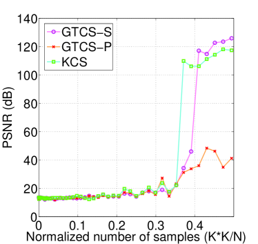
(a) PSNR comparison

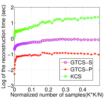
(b) Recovery time comparison

Figure 1: PSNR and reconstruction time comparison on sparse image.

(a) The original sparse image

(b) GTCS-S recovered image

(c) GTCS-P recovered image

(d) KCS recovered image

Figure 2: The original image and the recovered images by GTCS-S (PSNR = 22.28 dB), GTCS-P (PSNR = 23.26 dB) and KCS (PSNR = 22.28 dB) when $m=38$, using 0.35 normalized number of samples.

IV-B Compressible image representation

As shown in Figure 3(a), the cameraman image is resized to $64\times 64$ ($N=4096$ pixels). The image itself is non-sparse. However, in some transformed domain, such as discrete cosine transformation (DCT) domain in this case, the magnitudes of the coefficients decay by power law in both directions (see Figure 3(b)), thus are compressible. We let the number of measurements evenly split among the two modes. Again, in matrix data case, MWCS concurs with GTCS-P. We exhaustively vary $m$ from 1 to 64.

Figure 4(a) and 4(b) compare the PSNR and the recovery time respectively. Unlike the sparse image case, GTCS-P shows outstanding performance in comparison with all other methods, in terms of both accuracy and speed, followed by KCS and then GTCS-S. The reconstructed images when $m=46$, using 0.51 normalized number of samples and when $m=63$, using 0.96 normalized number of samples are shown in Figure 5.

(a) Cameraman in space domain

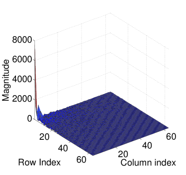
(b) Cameraman in DCT domain

Figure 3: The original cameraman image (resized to 64 $\times$ 64 pixels) in the space domain (a) and the DCT domain (b).

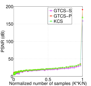
(a) PSNR comparison

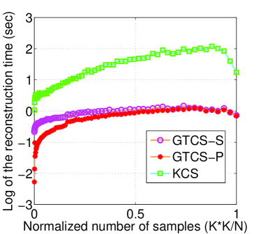
(b) Recovery time comparison

Figure 4: PSNR and reconstruction time comparison on compressible image.

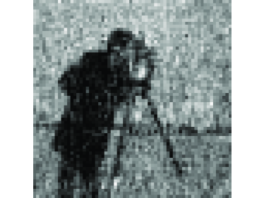
(a) GTCS-S, m= 46, PSNR = 20.21 dB

(b) GTCS-S, m = 63, PSNR = 30.88 dB

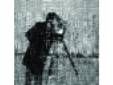
(c) GTCS-P/MWCS, m = 46, PSNR = 21.84 dB

(d) GTCS-P/MWCS, m = 63, PSNR = 35.95 dB

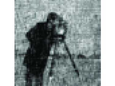
(e) KCS, m = 46, PSNR = 21.79 dB

(f) KCS, m = 63, PSNR = 33.46 dB

Figure 5: Reconstructed cameraman images. In this two-dimensional case, GTCS-P is equivalent to MWCS.

IV-C Sparse video representation

We next compare the performance of GTCS and KCS on video data. Each frame of the video sequence is preprocessed to have size $24\times 24$ and we choose the first 24 frames. The video data together is represented by a $24\times 24\times 24$ tensor and has $N=13824$ voxels in total. To obtain a sparse tensor, we manually keep only $6\times 6\times 6$ nonzero entries in the center of the video tensor data and the rest are set to zero. Therefore, the video tensor itself is $216$-sparse and its mode-$i$ fibers are all $6$-sparse for $i\in[3].$ The randomly constructed Gaussian measurement matrix for each mode is now of size $m\times 24$ and the total number of samples is $m^{3}$. Therefore, the normalized number of samples is $\frac{m^{3}}{N}$. In the decomposition stage of GTCS-P, we employ a decomposition described in Section II-A to obtain a weaker form of the core Tucker decomposition. We vary $m$ from 1 to 13.

Figure 6(a) depicts PSNR of the first non-zero frame recovered by all three methods. Please note that the PSNR values of different video frames recovered by the same method are the same. All methods exhibit an abrupt increase in PSNR at $m=10$ (using 0.07 normalized number of samples). Also, Figure 6(b) summarizes the recovery time. In comparison to the image case, the time advantage of GTCS becomes more important in the reconstruction of higher-order tensor data.

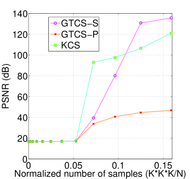
(a) PSNR comparison

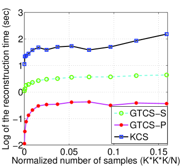
(b) Recovery time comparison

Figure 6: PSNR and reconstruction time comparison on sparse video.

We specifically look into the recovered frames of all three methods when $m=12$. Since all the recovered frames achieve a PSNR higher than 40 dB, it is hard to visually observe any difference compared to the original video frame. Therefore, we display the reconstruction error image defined as the absolute difference between the reconstructed image and the original image. Figures 7(a), 7(b), and 7(c) visualize the reconstruction errors of all three methods. Compared to KCS, GTCS-S achieves much lower reconstruction error using much less time.

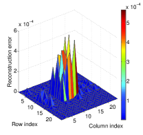
(a) Reconstruction error of GTCS-S

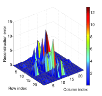
(b) Reconstruction error of GTCS-P

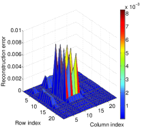
(c) Reconstruction error of KCS

Figure 7: Visualization of the reconstruction error in the recovered video frame 9 by GTCS-S (PSNR = 130.83 dB), GTCS-P (PSNR = 44.69 dB) and KCS (PSNR = 106.43 dB) when $m=12$, using 0.125 normalized number of samples.

To compare the performance of GTCS-P with MWCS, we examine MWCS with various tensor rank estimations and Figure 8(a) and Figure 8(b) depict its PSNR and reconstruction time respectively. The straight line marked GTCS is merely used to indicate the corresponding performance of GTCS-P with the same amount of measurements and has nothing to do with various ranks.

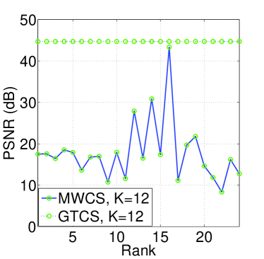
(a) PSNR comparison

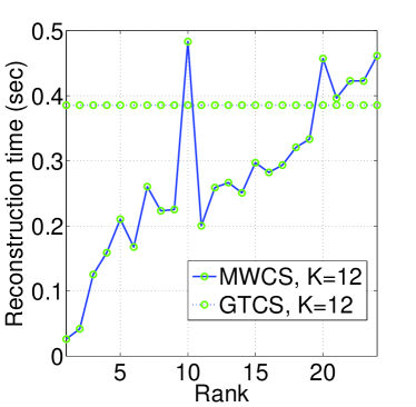
(b) Recovery time comparison

Figure 8: PSNR comparison of GTCS-P with MWCS on sparse video when $m=12$, using 0.125 normalized number of samples. The highest PSNR of MWCS with estimated tensor rank varying from 1 to 24 appears when Rank = 16.

IV-D Compressible video representation

We finally examine the performance of GTCS, KCS and MWCS on compressible video data. Each frame of the video sequence is preprocessed to have size $24\times 24$ and we choose the first 24 frames. The video data together is represented by a $24\times 24\times 24$ tensor. The video itself is non-sparse, yet compressible in three-dimensional DCT domain. In the decomposition stage of GTCS-P, we employ a decomposition described in Section II-A to obtain a weaker form of the core Tucker decomposition and denote this method by GTCS-P (CT). We also test the performance of GTCS-P by using HOSVD in the decomposition stage and denote this method by GTCS-P (HOSVD) hereby. $m$ varies from 1 to 21. Note that in GTCS-S, the reconstruction is not perfect at each mode, and becomes more and more noisy as the recovery by mode continues. Therefore the recovery method by $\ell_{1}$-minimization using (4) would be inappropriate or even has no solution at certain stage. In our experiment, GTCS-S by (4) works for $m$ from 1 to 7. To use GTCS-S for $m=8$ and higher, relaxed recovery (7) could be employed for reconstruction. Figure 9(a) and Figure 9(b) depict PSNR and reconstruction time of all methods up to $m=7$. For $m=8$ to 21, the results are shown in Figure 9(c) and Figure 9(d).

We specifically look into the recovered frames of all methods when $m=17$ and $m=21$. Recovered frames 1, 9, 17 (originally as shown in Figure 10) are depicted as an example in Figure 11.

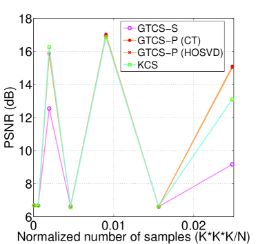
(a) PSNR comparison

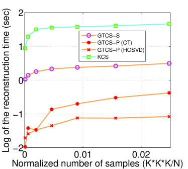
(b) Recovery time comparison

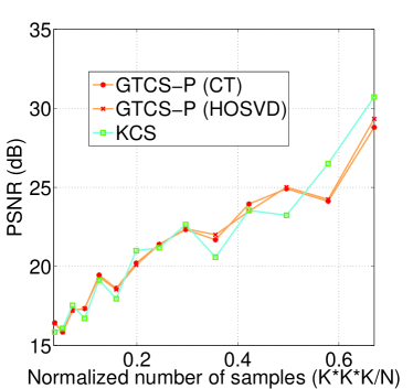
(c) PSNR comparison

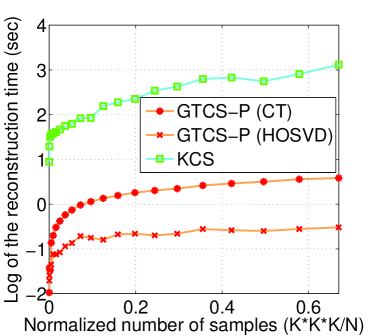
(d) Recovery time comparison

Figure 9: PSNR and reconstruction time comparison on susie video.

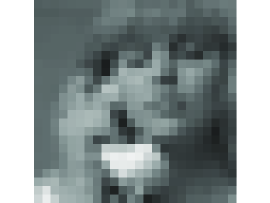
(a) Original frame 1

(b) Original frame 9

(c) Original frame 17

Figure 10: Original video frames.

(a) GTCS-P(HOSVD) reconstructed frame 1

(b) GTCS-P(HOSVD) reconstructed frame 9

(c) GTCS-P(HOSVD) reconstructed frame 17

(d) GTCS-P(CT) reconstructed frame 1

(e) GTCS-P(CT) reconstructed frame 9

(f) GTCS-P(CT) reconstructed frame 17

(g) KCS reconstructed frame 1

(h) KCS reconstructed frame 9

(i) KCS reconstructed frame 17

(j) MWCS reconstructed frame 1

(k) MWCS reconstructed frame 9

(l) MWCS reconstructed frame 17

Figure 11: Reconstructed video frames when m = 21 using 0.67 normalized number of samples by GTCS-P (HOSVD, PSNR = 29.33 dB), GTCS-P (CT, PSNR = 28.79 dB), KCS (PSNR = 30.70 dB) and MWCS (Rank = 4, PSNR = 22.98 dB).

As shown in Figure 12(a), the performance of MWCS relies highly on the estimation of the tensor rank. We examine the performance of MWCS with various rank estimations. Experimental results demonstrate that GTCS outperforms MWCS not only in speed, but also in accuracy.

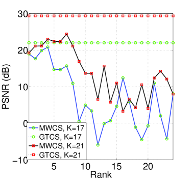
(a) PSNR comparison

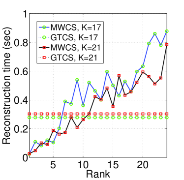
(b) Recovery time comparison

Figure 12: PSNR comparison of GTCS-P with MWCS on compressible video when $m=17$, using 0.36 normalized number of samples and $m=21$, using 0.67 normalized number of samples. The highest PSNR of MWCS with estimated tensor rank varying from 1 to 24 appears when Rank = 4 and Rank = 7 respectively.

V Conclusion

Extensions of CS theory to multidimensional signals have become an emerging topic. Existing methods include Kronecker compressive sensing (KCS) for sparse tensors and multi-way compressive sensing (MWCS) for sparse and low-rank tensors. We introduced the Generalized Tensor Compressive Sensing (GTCS)–a unified framework for compressive sensing of higher-order tensors which preserves the intrinsic structure of tensorial data with reduced computational complexity at reconstruction. We demonstrated that GTCS offers an efficient means for representation of multidimensional data by providing simultaneous acquisition and compression from all tensor modes. We introduced two reconstruction procedures, a serial method (GTCS-S) and a parallelizable method (GTCS-P), and compared the performance of the proposed methods with KCS and MWCS. As shown, GTCS outperforms KCS and MWCS in terms of both reconstruction accuracy (within a range of compression ratios) and processing speed. The major disadvantage of our methods (and of MWCS as well), is that the achieved compression ratios may be worse than those offered by KCS. GTCS is advantageous relative to vectorization-based compressive sensing methods such as KCS because the corresponding recovery problems are in terms of a multiple small measurement matrices $U_{i}$’s, instead of a single, large measurement matrix $A$, which results in greatly reduced complexity. In addition, GTCS-P does not rely on tensor rank estimation, which considerably reduces the computational complexity while improving the reconstruction accuracy in comparison with other tensorial decomposition-based method such as MWCS.