Outflow forces of low mass embedded objects in Ophiuchus: a quantitative comparison of analysis methods

Abstract

Context. The outflow force of molecular bipolar outflows is a key parameter in theories of young stellar feedback on their surroundings. The focus of many outflow studies is the correlation between the outflow force, bolometric luminosity and envelope mass. However, it is difficult to combine the results of different studies in large evolutionary plots over many orders of magnitude due to the range of data quality, analysis methods and corrections for observational effects such as opacity and inclination.

Aims. We aim to determine the outflow force for a sample of low luminosity embedded sources. We will quantify the influence of the analysis method and the assumptions entering the calculation of the outflow force.

Methods. We use the James Clerk Maxwell Telescope to map ¹²CO $J$=3–2 over 2$\arcmin\times 2\arcmin$ regions around 16 Class I sources of a well-defined sample in Ophiuchus at 15$\arcsec$ resolution. The outflow force is then calculated using seven different methods differing e.g. in the use of intensity-weighted emission and correction factors for inclination. Two well studied outflows (HH 46 and NGC1333 IRAS 4A) are added to the sample and included in the comparison.

Results. The results from the analysis methods differ from each other by up to a factor of 6, whereas observational properties and choices in the analysis procedure affect the outflow force by up to a factor of 4. Subtraction of cloud emission and integrating over the remaining profile increases the outflow force at most by a factor of 4 compared to line wing integration. For the sample of Class I objects, bipolar outflows are detected around 13 sources including 5 new detections, where the three non-detections are confused by nearby outflows from other sources. New outflow structures without a clear powering source are discovered at the corners of some of the maps.

Conclusions. When combining outflow forces from different studies, a scatter by up to a factor of 5 can be expected. Although the true outflow force remains unknown, the separation method (separate calculation of dynamical time and momentum) is least affected by the uncertain observational parameters. The correlations between outflow force, bolometric luminosity and envelope mass are further confirmed down to low luminosity sources.

1 Introduction

Molecular outflow activity begins early during the formation process of low-mass protostars and is therefore a tracer of active star formation (Bachiller & Tafalla 1999; Arce & Sargent 2006). Outflows actively contribute to the core collapse and formation of the star by carrying away angular momentum that would otherwise prevent accretion (Bachiller 1996; Hogerheijde et al. 1998). The strength of an outflow is measured by the outflow force $F_{\rm CO}$: the ratio of the momentum and the dynamical age of the outflow (Bachiller & Tafalla 1999). It is a measure of the rate at which momentum is injected into the envelope by the protostellar outflow (Downes & Cabrit 2007). The outflow force has been used to understand the driving mechanism of outflows. The correlation between the bolometric luminosity $L_{\rm bol}$ and outflow force suggests that a single mechanism is responsible for driving the outflow, at least partly related to accretion (Cabrit & Bertout 1992). A second correlation between $F_{\rm CO}$ and $M_{\rm env}$ (Bontemps et al. 1996) underlines the evolutionary properties of this parameter, suggesting that the outflow activity declines during the later stages of the accretion phase though this is more difficult to separate from initial conditions (Hatchell et al. 2007). Due to these correlations, the outflow force is a very important parameter for understanding the physical processes underlying the early phases of star formation.

Outflow forces have been derived for many embedded sources over the past 30 years using various methods and with continuous increase of observational resolution and $S/N$, resulting in a very inhomogeneous data set. Outflow properties for low-mass protostars have been compared in population studies of entire star forming regions and in different phases of evolution, ranging from the deeply embedded Class 0 to the T Tauri Class II stage (Cabrit & Bertout 1992; Bontemps et al. 1996; Richer et al. 2000; Arce & Sargent 2006; Hatchell et al. 2007). A central focus of many of these studies are the evolutionary trend plots of $F_{\rm CO}$ versus $L_{\rm bol}$ and $F_{\rm CO}$ versus $M_{\rm env}$ as described above. However, the results of these studies cannot usually be combined into a single dataset including all nearby clouds due to the range of data quality, the different methods used to determine outflow properties and the different corrections for observational effects, such as opacity and inclination, that have been applied. For individual targets, different methods have been shown to result in different values of the outflow force up to an order of magnitude (Hatchell et al. 2007). Comparisons in the value of the outflow force with different CO transitions (e.g. $J$=1–0, 2–1, 3–2, 6–5) show similar results (van Kempen et al. 2009a; Nakamura et al. 2011; Yıldız et al. 2012) . Although some comparison studies with outflow models exist (Cabrit & Bertout 1992, CB92 hereafter; Downes & Cabrit 2007, DC07 hereafter), the influence of the analysis method itself and the assumptions entering the calculation have never been quantified systematically against a single set of observational data.

The $\rho$ Oph molecular cloud complex ($d\sim 120\pm 4$ pc; Loinard et al. 2008) is one of the nearest and best studied star forming regions (Lada & Wilking 1984; Greene et al. 1994). Tens of young stellar objects (YSOs) have been identified, especially in the main filament L1688 (Wilking et al. 2008, and references therein). Due to the clustering of star formation in Ophiuchus, the YSOs are very close together and their outflows sometimes overlap along the line of sight (e.g. Bussmann et al. 2007). Class I outflows in Ophiuchus have been studied extensively and their properties have been obtained for many sources (Bontemps et al. 1996; Sekimoto et al. 1997; Kamazaki et al. 2001, 2003; Ceccarelli et al. 2002; Boogert et al. 2002; Bussmann et al. 2007; Gurney et al. 2008; Zhang & Wang 2009; Nakamura et al. 2011). Additional studies of YSOs in Ophiuchus from earlier data, including sources with outflows, are summarized in Wilking et al. (2008). It has been suggested that star formation in Ophiuchus was triggered by supernovae, ionization fronts and winds from the Upper Scorpius OB association, located to the west of the Ophiuchus cloud (Preibisch & Zinnecker 1999; Nutter et al. 2006) and started in the denser northwestern L1689 region (Zhang & Wang 2009).

In a recent study by van Kempen et al. (2009c), a number of YSOs in Ophiuchus were classified as so-called ‘Stage 1’ sources, using a new classification based on $M_{\rm disk}$, $M_{\rm env}$ and $M_{\rm star}$. Since this classification relies on physical rather than observational parameters (c.f. Lada classification, with spectral slope $\alpha_{\rm IR}$, Lada & Wilking 1984), this sample represents a well-defined embedded YSO sample in this cloud and outflow activity is expected to be detected from every source. For about half of these sources bipolar outflows were identified previously, but not with the high spatial resolution of 15$\arcsec$ that is available with the HARP array receiver (Buckle et al. 2009) at the James Clerk Maxwell Telescope (JCMT). High-resolution ¹²CO $J$=3–2 spectral maps offer the means to study the occurence, origin and properties of the outflows in more detail than previous studies. Therefore, this data set is perfect to systematically study and quantify the effect of different analysis methods. The sources are also part of the Herschel key programs “Water in Star-forming Regions with Herschel” (WISH) and “Dust, Ice and Gas In Time” (DIGIT) (van Dishoeck et al. 2011, Green et al. (in prep.)): complementary data on feedback based on far infrared line emission will become available in the following years for comparison.

This paper presents the results of a comparison between analysis methods of the outflow force with CO spectral maps, applied to 13 sources in Ophiuchus and two additional, well-studied outflows: HH 46 (van Kempen et al. 2009a) and NGC1333 IRAS 4A (Yıldız et al. 2012). The outline of this paper is as follows. In Sect. 2, the details of the observations and basic data reduction are discussed. Section 3 presents the spectral profiles and contour maps of the integrated line wings, indicating the outflow lobes. In Sect. 4, the results of the various outflow force analysis methods are presented and discussed. Section 5 discusses the comparison of outflow force values with those found in the literature, the trends of the outflow parameters and its implications for evolutionary models and the comparison of outflow morphologies with observed disks. The conclusions of the paper are given in Sect. 6.

2 Observations

2.1 Sample selection

The 16 ‘Stage 1’ sources identified by van Kempen et al. (2009c) were selected for the sample of this outflow study, out of a sample of 41 sources with potential Class I classification ($\alpha_{\rm 2-24\mu{}m}>$ 0.3 and $T_{\rm bol}<$ 650 K). Figure 1 presents an overview of our sample, the basic properties of which are shown in Table 1. IRS 46 is classified as Stage 2, but an outflow was also detected for this source in this study. The $L_{\rm bol}$ for this sample ranges from 0.04 to 14.1 $L_{\odot}$. Except for IRS 63, all sources are located in the L 1688 ridge.

Figure 1 shows an overview of the bipolar outflows and their relative positions in the L1688 core in Ophiuchus, where each square represents a spectral map and the red and blue arrows show the direction and extent of the red and blue outflows. VLA 1623 is added as well, based on figures in Yu & Chernin (1997). The background shows the 850 $\mu$m SCUBA map as published by Johnstone et al. (2000) and Di Francesco et al. (2008). IRS 63 lies outside the borders of this map and is presented as inset.

Table 1: Sample of Stage 1 sources in Ophiuchus.

Source	Coordinates (J2000)		Alternative names	$L_{\rm bol}$	$M_{\rm env}$	$i$
	RA	Dec		($L_{\odot}$)	(10-2 $M_{\odot}$)	($\degr$)
GSS 30-IRS1	16:26:21.4	$-$24:23:04.1	GSS 30, Elias 21	3.3	20.5	-
GSS 30-IRS3	16:26:21.7	$-$24:22:51.4	LFAM 1	0.83	17.1	-
WL 12	16:26:44.0	$-$24:34:48.0	GY 111	3.4	4.6	30
LFAM 26	16:27:05.3	$-$24:36:29.8	GY 197, CRBR 2403.7	0.04	4.5	70
WL 17	16:27:07.0	$-$24:38:16.0	GY 205	0.67	4.0	50
Elias 29	16:27:09.6	$-$24:37:21.0	WL15, GY 214	14.1	4.0	50
IRS 37	16:27:17.6	$-$24:28:58.0	GY 244	0.38	1.2	50
WL 3	16:27:19.3	$-$24:28:45.0	GY 249	0.46	2.9	-
WL 6	16:27:21.8	$-$24:29:55.0	GY 254	0.85	$<$0.4	50
IRS 43	16:27:27.1	$-$24:40:51.0	GY 265, YLW 15	1.0	17.1	10
IRS 44	16:27:28.3	$-$24:39:33.0	GY 269	1.1	8.0	30
IRS 46	16:27:29.7	$-$24:39:16.0	GY 274	0.19	3.3	50
Elias 32	16:27:28.6	$-$24:27:19.8	IRS 45, VSSG 18	0.5	41.9	-
Elias 33	16:27:30.1	$-$24:27:43.0	IRS 47, VSSG 17	1.2	28.2	70
IRS 54	16:27:51.7	$-$24:31:46.0	GY 378	0.78	3.1	50
IRAS 16253–2429	16:28:21.6	$-$24:36:23.7		0.06	10.3	70
IRS 63	16:31:35.7	$-$24:01:29.5	GWAYL 4	1.0	30.0	30

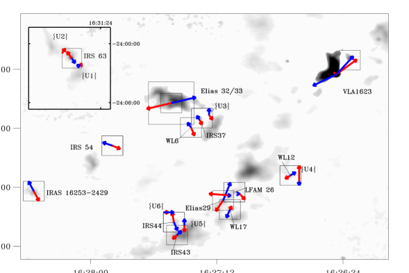
Figure 1: The L1688 core in Ophiuchus and the region around IRS 63 (inset upper left corner). The background shows the 850 $\mu$m SCUBA map (Johnstone et al. 2000; Di Francesco et al. 2008). The locations of all observed HARP maps are indicated by squares, labeled by the sources within. The blue and red arrows indicate the direction and observed extent of the blue and red outflow of that source, except for the extent of VLA 1623, which was taken from Yu & Chernin (1997) who observed the region centered at VLA 1623. In crowded regions, lines connect the source names to the origin location of the outflow. Newly detected outflow structures without a driving source are marked with Us.

2.2 ¹²CO maps of Ophiuchus

All sources were observed in the $J$=3–2 line of ¹²CO (345.796 GHz) with the HARP array receiver at the James Clerk Maxwell Telescope (JCMT) as part of program M08AN05. A bandwidth of 250 MHz was used with the ACSIS backend, resulting in a native spectral resolution of 0.026 km s^-1. The observations were carried out in June 2008 under weather conditions with an atmospheric opacity $\tau_{\rm 225GHz}$ ranging from 0.08 to 0.12. For analysis of the line wings, the spectra are typically binned to 0.1 km s^-1, giving $\sigma_{\rm rms}$ = 0.2 K. The HARP array consists of 16 receivers arranged in a 4$\times$4 pattern, mapping the sources over 2$\arcmin\times 2\arcmin$ to capture the full extent of the outflows with 15$\arcsec$ spatial resolution. The maps were made in the jiggle observing mode and resampled with a pixel size of 7$\aas@@fstack{\prime\prime}$5. A position switch of 60$\arcmin$ or 150$\arcmin$ was used. For one night, the reference off position accidentally coincided with emission, resulting in negative absorption troughs in the spectra in the maps of Elias 32 and Elias 33, IRS 37, IRS 43, IRS 44, LFAM 26, WL 17 and IRS 54. This has, however, no influence on the study of line wings. The Class 0 source IRAS 16293–2422 was used as a line calibrator. The main-beam efficiency was 0.63 and pointing errors were within 2$\arcsec$. Two receivers were broken at the time of observation (H03 and H014), resulting in lack of data in the south-east and the north-north-west corner of each map. Some sources are separated by less than 30$\arcsec$ and were therefore mapped in a single image (Elias 32 + Elias 33; IRS 37 + WL 3; GSS30-IRS1 + GSS30-IRS3; and IRS 44 + IRS 46). Only for the last case the two sources could be analyzed separately. In addition, Elias 33 was observed in September 2007 with HARP in the raster observing mode. This source was mapped in a 4$\arcmin\times 4\arcmin$ region and resampled to a pixel size of 12$\arcsec$. Atmospheric opacity was 0.05. The rms noise $\sigma_{\rm rms}$ for the rebinned spectra is again 0.2 K in 0.1 km s^-1 bins.

2.3 ¹³CO spectra

In order to determine the optical depth of the line wings of the outflows additional ¹³CO $J$=3–2 (330.58797 GHz) spectra were taken for two of the strongest outflows (Elias 29 and IRS 44) at the central positions. The HARP array receiver at the JCMT was used in the same setup as the ¹²CO observations as single pointings instead of jiggle maps. The observations were carried out in March 2011 as part of program M10BN05 under weather conditions with an opacity $\tau_{\rm 225GHz}$ of $\sim$0.11. The rms noise $\sigma_{\rm rms}$ for the reduced spectra is 0.05 K in 0.4 km s^-1 bins. Although all 16 receivers recorded a spectrum, only the spectrum at the central position showed line wings and so could be used for the optical depth derivation of the ¹²CO line wings. This will be discussed further in Sect. 3.3.

2.4 ¹²CO maps of HH46 and IRAS4A

For the outflow analysis comparison, ¹²CO $J$=3–2 datasets published in van Kempen et al. (2009a) and Yıldız et al. (2012) of HH 46 and IRAS 4A were used, respectively. The HH 46 observations were taken at the Atacama Pathfinder EXperiment (APEX), regridded to a map of $2\arcmin\times 2\arcmin$ and have a typical rms noise of 0.6 K in 0.2 km s^-1 bins. The observations of IRAS 4A were taken in jiggle mode with the HARP array receiver at the JCMT, regridded to a map of $4\arcmin\times 4\arcmin$ have a typical rms noise of 0.15 K in 0.1 km s^-1 bins. For more details on these observations, see the original references.

3 Results

3.1 Spectral profiles

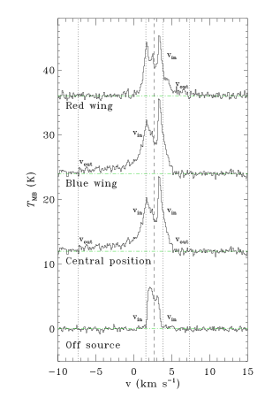
Figure 2: ¹²CO 3–2 spectra toward IRS 63, from top to bottom: one red outflow lobe position (15$\arcsec$,15$\arcsec$), one blue outflow lobe position (0$\arcsec$, $-$7$\aas@@fstack{\prime\prime}$5), the central position (0$\arcsec$,0$\arcsec$) and one off-source position ($-$42$\aas@@fstack{\prime\prime}$5,20$\arcsec$). The integration limits are marked by dotted lines, baselines by dash-dotted lines and the source velocity by a dashed line.

¹²CO $J$=3–2 is detected towards all sources, showing broad line profiles centered around $\varv_{\rm LSR}\sim$4 km s^-1. An example set of spectra is shown in Fig. 2 for IRS 63. The spectral profiles consist of red/blue-shifted wing emission from the outflow, central emission peaks from cloud and envelope material or foreground layers and narrow absorption features caused by self-absorption. At the outflow positions, broad line wings are detected, up to +15 km s^-1 in the red and $-$10 km s^-1 in the blue.

3.2 Outflow maps

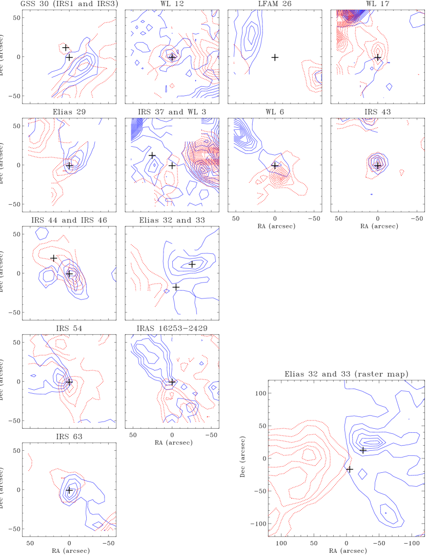
Figure 3: Outflow maps of all sources. Contours are drawn based on the integrated intensities of the line wings. Contours are drawn at 20, 40, 60, 80 and 100% of the peak value of the integrated intensity of the target source. The source positions are marked by pluses. Two receivers were broken at the time of observation, resulting in lack of data in the south-east and north-north-west corner of each map. In maps with Elias 32 and 33, Elias 32 is north west of Elias 33. In the GSS 30 map, GSS 30-IRS3 is north of GSS 30-IRS1. In the IRS 37 map, WL 3 is east of IRS 37. In the IRS 44 map, IRS 46 is north east of IRS 44.

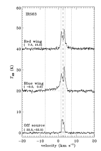
(m)

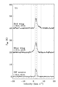
(n)

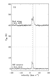
(o)

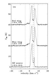
(p)

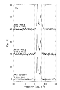
(q)

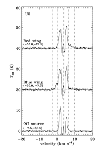
(r)

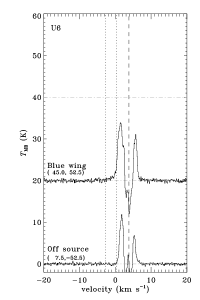
(s)

Figure 11: Overview of relevant outflow spectra - Continued

Outflow maps were made of the integrated CO wing emission in blue and red velocity intervals. The integration limits were chosen as follows. For each position, the outer velocity, $\varv_{\rm out}$, is defined as the velocity where the emission is still above the 1$\sigma$ rms level in 0.1 km s^-1 bins. The inner velocity limits, $\varv_{\rm in}$, in each map are defined as the $\varv_{\rm out}$ in an off-source ¹²CO spectrum (see Fig. 2 for the example of IRS 63). The blue wing integration limits typically range from $-$6 km s^-1 to +1 km s^-1, and for the red wing from 6 km s^-1 to 12 km s^-1 (see Fig. 11). Contour maps of the integrated outflow emission are presented in Fig. 3.

The maps show outflow activity in most of the sources. Infrared source positions are at (0$\arcsec$,0$\arcsec$) or marked when there are multiple sources. Most outflows fit in the 2$\arcmin\times 2\arcmin$ region, except for Elias 32/33, Elias 29, LFAM 26 and IRAS 16253–2429, although the outflow direction can still be recognized. Elias 32/33 is also observed in the raster mode in 4$\arcmin\times 4\arcmin$ maps, covering a larger part of the outflow (see lower right panel in Fig. 3).

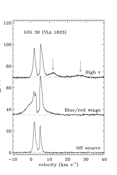
Figure 12: Spectrum with extremely high velocity (EHV) emission in the GSS 30 map as indicated by arrows, originating from the Class 0 source VLA 1623. Any outflow emission from GSS 30 itself can not be disentangled from VLA 1623 in the present observations. From top to bottom: one high velocity position ($-$45$\arcsec$, 0$\arcsec$), one wing position ($-$30$\arcsec$, $-$22$\aas@@fstack{\prime\prime}$5) and one off-source position (37$\aas@@fstack{\prime\prime}$5, 22$\aas@@fstack{\prime\prime}$5). The baselines are marked by dashed lines. The high-velocity bullet at 28 km s^-1 has not been identified in earlier studies of VLA 1623.

Bipolar outflows are seen for 13 sources (see Table 2), although nearby outflows complicate the view in several cases. In the Elias 29 map, emission from the east lobe of LFAM 26 is seen in the upper right corner, while part of the blue lobe of Elias 29 falls in the LFAM 26 map and the red lobe in the WL 17 map. A full coverage of these two outflows can be found in Bussmann et al. (2007) and Nakamura et al. (2011). The red lobe of Elias 32/33 extends all the way to IRS 54 and the blue lobe is wide enough to show close to WL 6 (Nakamura et al. 2011). The lobes of IRS 44 extend into the IRS 43 map. In the map containing GSS 30, the outflow emission is completely dominated by the 15$\arcmin$ long outflow extending from VLA 1623, a Class 0 source at 16:26:26.26, $-$24:24:30.01 (Andre et al. 1993; Dent et al. 1995; Yu & Chernin 1997). A high-velocity bullet (Bachiller & Tafalla 1999) at 28 km s^-1, not identified in earlier studies of VLA 1623, was discovered 50$\arcsec$ south of GSS 30 (see Fig. 12). Jørgensen et al. (2009) resolved an outflow lobe for GSS 30-IRS1 in interferometry HCO⁺ $J$=3–2 observations, tracing the inner outflow cone, but our CO observations do not reveal this outflow. In the case of Elias 29 and Elias 32/33, the red and blue lobes overlap with the pixels from the broken receivers, thus possibly underestimating the total outflow mass.

In the maps of Elias 32/33 and IRS 37/WL 3, only one set of outflow lobes was resolved: for this study they were assigned to Elias 33 and IRS 37, respectively. In the map of IRS 44, the Class II source IRS 46 is located 20$\arcsec$ north-east of IRS 44. Based on the sudden change of shape of the line wings, the spectral map was cut in two, assigning one half to IRS 46 and one half to IRS 44, each with their own bipolar outflow. In the maps containing IRS 37, IRS 44, IRS 63 and WL 12 new outflow structures were discovered which could not be assigned to an IR source. These structures were assigned U1, U2, etc. and are discussed further in Appendix A.

Based on the outflow maps in Fig. 3, an outflow status can be assigned to each source, which is listed in Table 2. Four new outflows were identified and nine were confirmed from previous observations.

Table 2: Outflow status for the 16 sources in this sample.

Source	Outflow status	References
GSS 30$-$IRS1	C	…
GSS 30$-$IRS3	C	…
WL 12	B	1
LFAM 26	B	2,3
WL 17	B	New
Elias 29	B	1,2,3,4
IRS 37	B	New
WL 3	C	…
WL 6	B	1,4
IRS 43	B	1
IRS 44	B	1,4
IRS 46	B	New
Elias 32/33	B	3,5
IRS 54	B	New
IRAS 16253–2429	B	New
IRS 63	B	1

(1) Bontemps et al. (1996), (2) Bussmann et al. (2007), (3) Nakamura et al. (2011), (4) Sekimoto et al. (1997), (5) Kamazaki et al. (2003).

3.3 Optical depth

The optical depth, $\tau$, is obtained from the line ratio of ¹²CO $J$=3–2 and its isotopolog ¹³CO $J$=3–2 for the central position of the outflows with the strongest line wings, Elias 29 and IRS 44. In Fig. 4, spectra of ¹²CO $J$=3–2 and ¹³CO $J$=3–2 at the central positions are shown, binned to 0.42 km s^-1, together with the ratio of ¹²CO $J$=3–2/¹³CO $J$=3–2. The optical depth for the line wings is derived assuming that the two species have the same excitation temperature and that the ¹³CO line wing is optically thin, using (Goldsmith et al. 1984):

$$\frac{I(^{12}{\rm CO})}{I(^{13}{\rm CO})}=\frac{1-e^{-\tau_{12}}}{1-e^{-\tau_{13}}}\approx\frac{1-e^{-\tau_{12}}}{\tau_{12}}\times R$$ (1)

with $R=\tau_{12}/\tau_{13}$ the abundance ratio ¹²CO/¹³CO (a ratio of 65 is assumed here, following Vladilo et al. 1993). The resulting optical depths of ¹²CO as a function of velocity are shown on the right-hand axes of the lower panels of Fig. 4. High optical depths $>$2 are found at velocities very close to the source velocity $\varv_{\rm source}$ implying that the central velocities are optically thick and become optically thinner away from the line center where the outflow emission starts. The only exception is the blue wing of IRS 44, which remains optically thick for 3 km s^-1 beyond $\varv_{\rm in}$. Quantitatively, the optical depth implies that the mass of the blue lobe at this single position is underestimated by a factor of 6 if the wing emission is assumed to be optically thin. At the other positions with ¹³CO measurements, the blue wing is still optically thin, so the total blue mass is not expected to increase more than a factor of 2 due to optical depth effects. Since the uncertainties on the outflow force are within a factor of a few, the impact of optical depth is negligible. Therefore outflow emission is assumed to be optically thin for all sources.

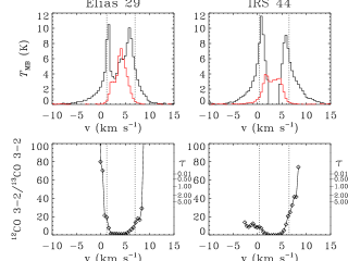
Figure 4: ¹²CO 3–2 and ¹³CO 3–2 spectra of the central position of Elias 29 (left) and IRS 44 (right). The top figure shows the spectra, binned to 0.42 km s^-1, the bottom figure shows the $T_{\rm MB}$ ratio of ¹²CO 3–2/¹³CO 3–2 and the corresponding optical depth $\tau$ on the right axis. The dotted lines show the integration limits, indicating the velocities $\varv_{\rm in}$ where the line wings start.

4 Outflow analysis

4.1 Outflow parameters

The main physical parameters of the outflow are the mass, $M$, the velocity, $\varv_{\rm CO}$ (defined as $|\varv_{\rm out}-\varv_{\rm source}|$, with $\varv_{\rm out}$ the outer velocity of the outflow emission at a given location), and the projected size of the lobe $R_{\rm lobe}$, for both the blue and red lobe. The mass is calculated from the integrated intensity of the ¹²CO line assuming an excitation temperature of 50 K (e.g. Yıldız et al. 2012) and the procedure explained in Appendix C. With these basic physical quantities the outflow force, $F_{\rm CO}$, can be derived as

$$F_{\rm CO}=\frac{M\varv_{\rm CO}^{2}}{R_{\rm lobe}}$$ (2)

The velocity, $\varv_{\rm CO}$, often called $\varv_{\rm max}$, is not a well-constrained parameter: due to the inclination and the shape of the outflow, often following a bow shock including forward and transverse motion, the measured velocities along the line of sight are not necessarily representative of the real velocities driving the outflow (Cabrit & Bertout 1992). This is the main reason why various methods have been developed to derive the outflow force, where a correction factor is often applied to compensate for these effects.

4.2 Analysis methods

Seven different methods for deriving the outflow force are analytically described in this section, with references to the paper where the method was originally presented. The constant $K$ refers to Equation 13. The following general recipe applies to each method for the blue and red lobe separately. The outflow parameters are calculated by adding up the absolute values for the blue and red lobe.

1. For each pixel, $j$, the outer velocity $\varv_{{\rm out},j}$ is defined as the outer velocity where the emission is still above the 1$\sigma$ rms level.

2. The inner velocity, $\varv_{\rm in}$, in each map is defined as the velocity in the average off-source ¹²CO spectrum where the emission is still above 5% of the peak emission $T_{\rm peak}$. $\varv_{\rm in}$ and $\varv_{{\rm out},j}$ define the integration limits for each line wing, the same $\varv_{\rm in}$ is used for each pixel.

3. The source velocity, $\varv_{\rm source}$, is determined using a high-density tracer such as HCO⁺ or a minor isotopologue with a non-self-absorbed profile. $\varv^{\prime}=\varv-\varv_{\rm source}$ is defined as the relative velocity.

4. Only pixels that are contributing to the outflow of the target are included to avoid confusion with nearby outflows.

5. The inclination angle, $i$, is estimated from the morphology of the contour map to be pole on (10$\degr$), inclined (30$\degr$ or 50$\degr$) or in the plane of the sky (70$\degr$), using Fig. 1-4 in Cabrit & Bertout (1990).

6. $R_{\rm lobe}$ is measured as the projected length of the outflow lobe.

7. The conversion from integrated intensity to mass is a multiplication with constant $K$ as defined in Appendix C.

Table 3: Correction factors.

$i$($\degr$)	10	30	50	70	Ref.
$c_{1}$	0.28	0.45	0.45	1.1	1,2
$c_{2}$	1.6	3.6	6.3	14.55	1
$c_{3}$	1.2	2.8	4.4	7.1	3

(1) Cabrit & Bertout (1990), (2) CB92, (3) Downes & Cabrit (2007).

4.2.1 $\varv_{\rm max}$ method (M1)

M1 is one of the most common methods in the literature (e.g. Cabrit & Bertout 1992; Hogerheijde et al. 1998; Downes & Cabrit 2007; van Kempen et al. 2009b). It assumes a constant $\varv^{\prime}_{\rm max}={\rm max}(\varv^{\prime}_{{\rm out},j})$ throughout the spectral map. The derived outflow force, $F_{\rm obs}$, is multiplied by the inclination correction factors $c_{1}(i)$ (see Table 3) derived by Cabrit & Bertout (1990, 1992) for $\varv_{\rm CO}$ to obtain $F_{\rm CO}$:

$$F_{\rm CO}=c_{1}\frac{K\left(\displaystyle\sum\limits_{j}\left[\int T(\varv){\mathrm{d}}\varv\right]_{j}\right){\varv^{\prime}}_{\rm max}^{2}}{R_{\rm lobe}}$$ (3)

4.2.2 $\varv_{\rm spread}$ method (M2)

In M2, $\varv_{{\rm out},j}$ is derived as a function of position (Yıldız et al. 2012). The local energy $M\varv_{{\rm CO},j}^{2}$ is calculated for each position in the map with the local velocity. No correction factors are applied:

$$F_{\rm CO}=\frac{K\left(\displaystyle\sum\limits_{j}{\varv^{\prime}}_{{\rm out},j}^{2}\times\left[\int T(\varv){\mathrm{d}}\varv\right]_{j}\right)}{R_{\rm lobe}}$$ (4)

4.2.3 $\langle\varv\rangle$ method (M3)

M3 uses intensity-weighted velocities by including $\varv^{\prime}$ in the integral (Cabrit & Bertout 1990; Downes & Cabrit 2007). The derived outflow force is multiplied by the inclination correction factors $c_{2}(i)$ (Table 3) derived in Cabrit & Bertout (1990) for $\langle\varv\rangle$ to obtain $F_{\rm CO}$:

$$F_{\rm CO}=c_{2}\times K\left(\frac{\left\{\displaystyle\sum\limits_{j}\left[\int T(\varv^{\prime})\varv^{\prime}{\mathrm{d}}\varv^{\prime}\right]_{j}\right\}^{2}}{R_{\rm lobe}\displaystyle\sum\limits_{j}\left[\int T(\varv^{\prime}){\mathrm{d}}\varv^{\prime}\right]_{j}}\right)\\$$ (5)

4.2.4 Local method (M4)

Using the kinematic structure of the outflow lobe, the local outflow force is calculated for each position by dividing the local energy $M\varv_{{\rm CO},j}^{2}$ by the projected distance $r_{j}$ between the position and source position (Lada & Fich 1996; Downes & Cabrit 2007). Hatchell et al. (2007) use a combination of M4 and M2, using projected distances and local velocities. No correction factors are applied:

$$F_{\rm CO}=K\left(\displaystyle\sum\limits_{j}\frac{\left[\int T(\varv^{\prime}){\varv^{\prime}}^{2}{\mathrm{d}}\varv^{\prime}\right]_{j}}{r_{j}}\right)$$ (6)

4.2.5 Perpendicular method (M5)

Because a large amount of the outflow material is moving slowly and predominantly in transverse motion, DC07 developed a method to determine the dynamical age, $t_{\rm d}$, of the outflow, using the half-width of the outflow lobe, $W_{\rm lobe}$, rather than the projected length. The factor $\frac{1}{3}$ (see below) originates from the asymptotic expansion of the bowshock wings, $R\propto t^{1/3}$ (DC07 and references therein). This method resulted in much more accurate estimates of the outflow force for the modeled outflows, but can only be applied in observations of spatially well-resolved outflows. In addition, since the models describe Class 0 sources, the results may not be applicable for outflows of Class I sources which are known to have large opening angles (e.g. Arce & Sargent 2006):

$$F_{\rm CO}=K\left(\frac{\left\{\displaystyle\sum\limits_{j}\left[\int T(\varv^{\prime})\varv^{\prime}{\mathrm{d}}\varv^{\prime}\right]_{j}\right\}^{2}}{\frac{1}{3}W_{\rm lobe}\displaystyle\sum\limits_{j}\left[\int T(\varv^{\prime}){\mathrm{d}}\varv^{\prime}\right]_{j}}\right)$$ (7)

4.2.6 Annulus method (M6)

In M6, the outflow force is calculated with a “slice” through the outflow (Bontemps et al. 1996). The momentum within an annulus or ring centered on the source position with thickness $\Delta{r}$ (equal to the beam size) and radius $r$ is measured, and the dynamical age is determined with $\Delta{r}$ rather than $R_{\rm lobe}$. The derived outflow force $F_{\rm obs}$ is multiplied by a mean correction factor $\langle f(i)\rangle=2.9$ with $f(i)=\sin i/\cos^{2}i$ and $\langle i\rangle\approx 57.3\degr$. Bontemps et al. (1996) applied an additional mean correction for the optical depth $\langle\tau_{\rm CO}(1-e^{-\tau_{\rm CO}})\rangle$ of 3.5 based on opacity values found by CB92, but opacity effects are not part of this comparison, so this factor is not included:

$$F_{\rm CO}=\langle f(i)\rangle\times\langle\frac{\tau_{\rm CO}}{1-e^{-\tau_{\rm CO}}}\rangle\times\frac{1}{\Delta{r}}\times K\left(\displaystyle\sum\limits_{j}\left[\int T(\varv^{\prime})\varv^{\prime 2}{\mathrm{d}}\varv^{\prime}\right]_{j}\right)\\$$ (8)

4.2.7 Separation method (M7)

In M7, the momentum and dynamical age are considered as separate parameters, with the dynamical age estimated using the maximum velocity, while the intensity-weighted velocity is a better measure for the momentum since it takes the kinematic structure into account (Downes & Cabrit 2007; Curtis et al. 2010). The dynamical age is corrected for inclination by using the ratios of $t_{\rm\varv_{max}}$/True age in Table 6 of Downes & Cabrit (2007). For these corrections, the geometrical mean for the mass density contrast $\eta=0.1$ and $\eta=1.0$ cases are taken for the first column in this table, and interpolated to correspond to the derived inclination angles, where $i=90-\alpha$ (see Table 3):

$$F_{\rm CO}=c_{3}\times\frac{K\left(\displaystyle\sum\limits_{j}\left[\int T(\varv^{\prime})\varv^{\prime}{\mathrm{d}}\varv^{\prime}\right]_{j}\right)\varv^{\prime}_{\rm max}}{{R_{\rm lobe}}}$$ (9)

4.2.8 Comparison of outflow force

All methods were applied to the same set of observations for all detected outflows in Ophiuchus, HH 46 and the Class 0 source IRAS 4A. For IRAS 4A, only the spectra within a 50$\arcsec$ radius are integrated to exclude “bullet” emission (Yıldız et al. 2012), see also Sect. D.0.2. Figure 5 summarizes the results, normalized to the $\varv_{\rm max}$ method (M1). Since the true outflow force remains unknown, all results are presented compared to this method. The sources are sorted by inclination angle, which is an important variable in determining an accurate outflow force (see Sect. 4.2.8).

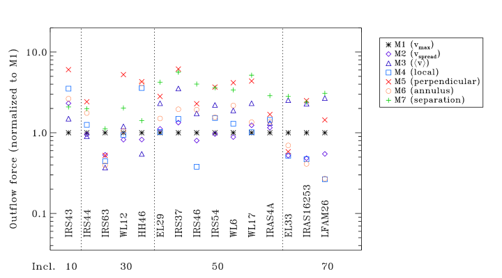
Figure 5: Outflow forces derived using different methods, normalized to the $\varv_{\rm max}$ method (M1), for all Ophiuchus Class I outflows and HH 46 and IRAS 4A. The sources are sorted by inclination angle.

Figure 5 shows the large dispersion of the resulting outflow force using different methods. All methods agree with each other within a factor of 6, with M5 and M7 giving systematically higher values than M1 with a mean factor M/M1 of 3.0, while M2, M3, M4 and M6 have mean factors of $\sim$1.5. M2 agrees very well with M1, implying that the correction factor $c_{1}$ taken from CB92 mainly compensates for the spread in velocity throughout the outflow lobe. The methods that do not involve correction factors (M2, M4, M5 and M6) result in lower values of the outflow force for the largest inclination angle with a factor of 2–3, but no other systematic effects related to inclination are found. IRAS 4A shows the smallest spread between methods, illustrating that the variations become less important when larger outflow velocities and smaller opening angles are involved such as usually found for Class 0 sources.

The largest uncertainties in the derivation of the outflow force are $\varv_{\rm max}$ and inclination. The velocity $\varv_{\rm max}$ is difficult to measure precisely since the shape of the outflow wings is almost exponential. The outflow force is less affected by the choice of $\varv_{\rm max}$ for M2, due to the local $\varv_{{\rm out},j}$, whereas the weighted velocity methods are only affected if the outer velocity limit is underestimated: an overestimate of $\varv_{\rm max}$ will not result in higher values since there is little emission at higher velocities. M1 has the largest uncertainty in this case since it depends quadratically on $\varv_{\rm max}$.

The inclination remains the biggest issue. Determining the inclination based on the morphology is fairly uncertain: generally one can only distinguish between pole-on, plane of the sky or something in between. A reasonable assumption is that $i=10\degr$ corresponds to $i\sim 0-30\degr$, $i=30\degr$ to $i\sim 30-50\degr$, $i=50\degr$ to $i\sim 30-70\degr$ and $i=70\degr$ to $i\sim 50-70\degr$, introducing intrinsic errors in M1, M3, M6 and M7. In addition, the correction factors that are based on models (M1, M3 and M7) are in themselves model-dependent, whereas outflow models are still relatively simple. M6 does not take individual inclinations into account and is therefore less accurate for the highest and lowest inclination. The correction factors from CB92 (M1, M3) are based on the spread in correction between a model of a high-velocity accelerated conical lobe surrounded by a slower envelope with three different velocity fields $\varv(r)$: $\varv(r)\propto 1/r$, $\varv(r)\propto r$ and $\varv(r)\propto{\rm constant}$. The correction factors from DC07 (M7) are based on a more advanced model: a protostellar jet model in an molecular cloud in a long-duration numerical simulation predicts the resulting outflow and its observed properties. DC07 also compares the outcome of M1 (including the corrections from CB92) and M3 (but without corrections) and they find that M1 is still correct to within a factor of 2 even though it was based on a much simpler model. M3, on the other hand, significantly underestimates the outflow force, especially for larger inclination angles, by at least a factor of 20 if no correction factor is applied while the correction factors based on the model from CB92 are only 1.2–7.1 (see Table 3) so these are clearly not sufficient. Surprisingly, the inclination dependence of M2 is weak, which would have been expected from the correction factors in M1.

In comparing these methods, it remains unclear which method best represents the true physical value of the outflow force, although the Class 0 outflow models of DC07 show that M3 and M4 (named global and local method in DC07) severely underestimate the physical outflow force and any applied correction factors are largely uncertain. In their case the outcome could be compared directly to the true force, as the energetic parameters are part of the model input. On the other hand, both M1 and M7 in the DC07 (using the dynamical time) matched reasonably well with the input models, using the inclination correction factors. From these two, M7 is least affected by inclination and choice of $\varv_{\rm max}$.

4.3 Outflow emission at ambient velocities

Another issue in outflow force analysis is the outflow material at ambient velocities, blending in with the low-velocity envelope material (DC07). In general, inner velocity limits are chosen at a few km s^-1 from the source velocity to exclude the bright and usually optically thick envelope emission, but in doing so some outflow material at low velocities is excluded. DC07 show that ignoring low-velocity material leads to an underestimate of the derived outflow momentum of typically a factor of 2–3 depending on the inner velocity limit and the maximum outer velocity. Some studies argue instead for subtraction of an off-source envelope spectrum and integration of the full remaining profile to obtain the outflow mass (e.g. Bontemps et al. 1996). The effect of subtraction of an envelope profile is investigated here (see Fig. 6), making good use of our HARP maps. The envelope profile is determined by averaging a number of off-source spectra, which are selected by eye from each map. This is not trivial in some of the Ophiuchus maps, due to the confusion with nearby outflows and foreground cloud emission. Typically, very little emission is left at ambient velocities after subtraction, although this is not the case for HH 46 and IRAS 4A. The remaining profile is integrated over all non-negative emission channels up to $\varv_{{\rm out},j}$.

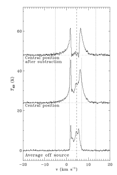
Figure 6: An example of an envelope-subtracted outflow ¹²CO 3–2 profile toward Elias 29. From bottom to top: the average of four off-source spectra in the Elias 29 map, the spectrum of the central position and the spectrum of the central position after subtraction of the averaged off-source spectra.

Figure 7 shows the results of this comparison. Systematic differences between the methods are clearly visible: the ratio is not larger than 2 for all intensity-weighted methods (M3–M6), while the outflow force can be up to a factor of 4 higher for the $\varv_{\rm max}$ method (M1). This is an intrinsic effect of the unweighted methods: all material, including that at ambient velocities, is multiplied with the high-velocity value, while the contribution of this material is less in the intensity-weighted methods. M7 follows a distribution between M1 and M3-M6 as it is only partly an intensity-weighted method. Still, including ambient material does not increase the outflow force by more than a factor of 5, which is lower than determined from the modeling results from DC07, who find factors up to 10–100. This can be understood as follows: by integrating the full profile (after subtraction), the total outflow mass is increased by the inclusion of the ambient outflow emission. However, in the derivation without subtraction some envelope emission is still included in the integration. These two factors add a comparable amount and therefore an analysis without subtraction does not automatically underestimate the mass.

Figure 7: Histogram of the ratio between the outflow force determination with subtraction of an envelope profile and without subtraction, for all sources in this study and for each method described in Section 4.2.

4.4 Other influences on the outflow force

Apart from the analysis method, the derived outflow force can be influenced by the data quality and choice of velocity limits. The effects are studied quantitatively in Appendix D. Although $\varv_{\rm max}$ depends on the data quality, the outflow force does not change more than a factor of 2 for small changes in the inner velocity limit, the rms level, the outer cut-off level and spectral binning even for the M1 method, which depends mostly on $\varv_{\rm max}$. It is also demonstrated that the spatial coverage in principle does not influence the outflow force, indicating that this is a conserved quantity along the outflow direction. The determination of the parameter $\varv_{\rm max}$ can also be affected by the quality of the baseline subtraction and thus instrumental effects and/or adopted observational techniques (e.g. on-the-fly mapping). The data and the baseline subtraction presented here is shown to be of excellent quality. However, if such quality is not apparent, one should be careful in the determination of $\varv_{\rm max}$. When combining the results from different studies, using different methods, assumptions and/or data quality, scatter up to a factor of 5 can be expected.

Measuring the size $R_{\rm lobe}$ from the observed CO gas makes the incorrect assumption that the gas has travelled at a constant speed from the protostar, whereas the observed CO is actually entrained from the environment and originates from the location where it has been accelerated. As long as acceleration occurs on $<$100 AU scales, the effect should be small. Modeling the effect of the environment on the measured outflow force is beyond the scope of this work.

4.5 Application to Ophiuchus

The basic outflow parameters (mass, size and velocity limits) are derived for each source, for both the blue and red lobes, using the main recipe described in Sect. 4.2. The source velocities were derived using HCO⁺ $J$=4–3 or C¹⁸O $J$=3–2 spectra from van Kempen et al. (2009c). The ¹²CO $J$=3–2 line wing is assumed to be optically thin and no off-source spectra were subtracted. These basic parameters are not corrected for inclination.

With the $\varv_{\rm max}$ method (M1) and the separation method (M7) the dynamical age and outflow force of all Ophiuchus sources are derived, the outflow force is corrected for inclination using the correction factors from CB92 and DC07. Although M7 is recommended for future derivation of outflow forces, the results from M1 are presented as well, as they will be combined with results from previous studies in evolutionary plots in Sect. 5.2. The new outflow structures without IR source (U1, U2, etc.) are analyzed in a similar way, although the parameters have a high uncertainty due to the poor spatial coverage. For the same reason, the inclination could not be derived for these outflows. The parameters for all outflows in Ophiuchus are given in Table 4. The outflow force for Elias 33 was derived for both the regular $2\arcmin\times 2\arcmin$ jiggle map and the larger $4\arcmin\times 4\arcmin$ raster map. In Table 4 only the first is given; it is within a factor of 2 with the derived value from the $4\arcmin\times 4\arcmin$ raster map with $F_{\rm CO}$ = 8.3$\cdot 10^{-6}M_{\odot}$ km s^-1 yr^-1, so consistent with the outflow force being a conserved quantity along the radius.

Table 4: Outflow parameters from ¹²CO observations for Ophiuchus sources.

		Blue lobe				Red lobe				M1	M7
Name	$\varv_{\rm source}$	$\varv^{\prime}_{\rm max}$	$R_{\rm lobe}$	$M$		$\varv^{\prime}_{\rm max}$	$R_{\rm lobe}$	$M$	$t_{\rm d}$	$F_{\rm CO}$	$F_{\rm CO}$
	(km s-1)	(km s-1)	(AU)	($M_{\odot}$)		(km s-1)	(AU)	($M_{\odot}$)	(yr)	($M_{\odot}$ km s-1	($M_{\odot}$ km s-1
										yr-1)	yr-1)
WL 12	4.3	6.1	7110	6.3($-$5)		6.8	5760	1.2($-$4)	4.8(3)	1.2($-$7)	2.5($-$7)
LFAM 26	4.2	5.2	3200	2.9($-$4)		12.8	6480	2.6($-$3)	3.7(3)	2.0($-$6)	5.5($-$6)
WL 17	4.5	5.0	7380	2.0($-$5)		5.3	4500	4.0($-$4)	5.5(3)	2.5($-$7)	1.3($-$6)
EL 29	4.6	9.8	4590	6.1($-$4)		8.8	4590	4.0($-$4)	2.3(3)	1.9($-$6)	0.8($-$5)
IRS 37	4.2	6.2	5130	0.9($-$4)		3.9	7830	4.4($-$4)	6.7(3)	1.4($-$7)	0.8($-$6)
WL 6	4.0	7.3	7650	2.0($-$4)		10.3	8550	6.2($-$4)	4.5(3)	0.9($-$6)	2.9($-$6)
IRS 43	3.8	7.7	4950	1.4($-$4)		7.3	5400	2.7($-$4)	3.3(3)	2.6($-$7)	5.5($-$7)
IRS 44	3.8	9.0	7650	4.7($-$4)		13.7	7740	1.2($-$3)	3.4(3)	3.2($-$6)	6.4($-$6)
IRS 46	3.8	7.5	5130	2.3($-$4)		10.3	4950	1.3($-$3)	2.8(3)	2.8($-$6)	1.1($-$5)
EL 33	4.5	11.2	8550	4.4($-$3)		5.8	6750	1.4($-$3)	4.6(3)	1.3($-$5)	3.7($-$5)
IRS 54	4.1	11.2	10260	3.3($-$4)		8.3	11520	2.5($-$4)	5.5(3)	0.9($-$6)	3.4($-$6)
IRAS 16253-2429	4.0	5.6	10170	1.4($-$4)		5.8	8910	5.3($-$4)	7.9(3)	5.7($-$7)	1.4($-$6)
IRS 63	2.7	10	5850	4.8($-$4)		4.6	6750	3.1($-$4)	4.9(3)	0.9($-$6)	1.0($-$6)
U1	2.7	4.9	5130	2($-$4)		4.6	4500	1.7($-$4)	4.8(3)	3.7($-$7)	1.8($-$7)
U2	2.7	…	…	…		3.3	1800	5.0($-$5)	2.6(3)	6.5($-$8)	4.4($-$8)
U3	4.2	8.8	7740	4.9($-$4)		4.8	7740	1.4($-$3)	5.9(3)	1.9($-$6)	0.9($-$6)
U4	4.3	4.6	7110	0.8($-$4)		4.7	12960	5.4($-$4)	1.0(4)	2.4($-$7)	1.4($-$7)
U5	3.8	6.2	2700	0.9($-$4)		6.0	2700	7.2($-$5)	2.1(3)	4.7($-$7)	4.4($-$7)
U6	3.8	6.4	3600	5.5($-$5)		…	…	…	2.6(3)	1.8($-$7)	1.4($-$7)

5 Discussion

5.1 Outflow characterization

Outflow activity has been associated with most of the embedded sources in this study. The only exceptions are outflows that are confused by other nearby outflows. Automatic line wing detection routines are not sufficient within clustered star formation such as Ophiuchus, especially when the envelope line profiles change within the star forming region. Earlier results of the non-detection of outflows may have been caused by the use of automatic line wing detection, low spatial resolution or low $S/N$. Since detailed inspection revealed bipolar outflows for every source in this study, it is likely that every embedded source has a bipolar outflow. This reinforces the protostellar nature of the newly detected outflow sources.

The sources for which no outflow could be identified due to confusion with another nearby source (Elias 32 and 33, IRS 37 and WL 3) are explored somewhat further. In this study, the driving source is determined based on morphology. Both sources may have outflows which are blended or along the same direction. In that case, the total outflow mass (and the outflow force) should be split up between the two sources.

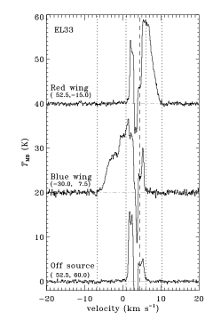
Figure 13: Outflow spectra of Elias 32/33, showing a red wing spectrum (top), blue wing spectrum (middle) and off-source spectrum (bottom). $\varv_{\rm source}$ (dashed line) and the integration limits (dotted lines) are indicated. A dash-dotted line indicates the baseline. Positions of each spectrum are indicated in brackets. Especially the blue wing shows a double structure, suggesting blending of outflow emission of two separate sources.

A closer look at the spectrum of Elias 33 (Fig. 13) shows a double structure in the line wings, especially the blue wing, with a high-intensity inner wing of 11 K and a low-intensity outer wing of 7 K, possibly indicating overlap of separate wings and suggesting blending of outflow emission of two separate sources. For IRS 37 and WL 3, the outflow force is not strong, but the envelope mass for both is $<$10 times that of Elias 33, suggesting more evolved YSOs. The outflow is however confused due to the missing data in the south east corner. Observations with full coverage will improve the possibility to assign this outflow to either one of the sources.

The bipolar outflow activity and outflow shape of all sources classified as ‘Stage 1’ in van Kempen et al. (2009c) do not contradict their classification methods. Outflows from more evolved Stage 2 sources are in general less bipolar and more wide-angled (Arce & Sargent 2006) than Stage 1, but the opening angle cannot be derived from our CO maps due to insufficient spatial resolution and low inclination. The difference between Stage 1 and Stage 2 can therefore not be confirmed by an outflow study, since Stage 2 sources may also show outflow activity, for example IRS 46 (in this study), IRS 48 and IRS 51 (Bontemps et al. 1996) and WL 10 (Sekimoto et al. 1997). No statistics are known for the occurrence of outflows with Stage 2 sources, but a non-detection would have been surprising for a Stage 1 source since all embedded protostars are expected to go through an outflow phase (Fukui et al. 1993; Arce & Sargent 2006).

When comparing the outflow forces derived in this paper with values in previous studies, significant differences are found, up to almost two orders of magnitude (see App. B). These differences can be explained to within a factor of a few by a detailed look into the methods and assumptions used previously. Since uncertainties in opacity and inclination potentially cause the largest variations in the outflow force, it is essential to derive these properties as accurately as possible.

Since the jet driving the outflow is assumed to originate from the spinning up of the magnetic field by the rotating disk, the outflow direction is perpendicular to the disk (Matsumoto & Tomisaka 2004). Therefore, the morphology of outflow and disk observations can be directly compared. In the last decade, very high spatial resolution observations revealing the disk structure of early phase YSOs have become available (Brinch et al. 2007; Lommen et al. 2008; Jørgensen et al. 2009) to which we compare the outflow results of this study.

The outflow of IRS 63 matches well with a disk inclination of 30$\degr$ and north-south orientation as was found with interferometric HCO⁺ $J$=3–2 observations (Lommen et al. 2008; Jørgensen et al. 2009). The outflow of IRS 46, which is in the plane of the sky, is also consistent with an edge-on disk, as was determined by fitting a disk model to the SED (Lahuis et al. 2006). In contrast, the outflow of Elias 29 is inconsistent with the interpretation of the HCO⁺ velocity gradient of Lommen et al. (2008) and Jørgensen et al. (2009), who argued that the blue-shifted and red-shifted emission are indicative of a disk ($i=30\degr$) in the north-north-west, south-south-east direction (see Jørgensen et al. 2009, Fig. 5). As this direction is parallel to the outflow emission, it is more likely that HCO⁺ is instead tracing the dense swept-up outflow material, indicating a small jet very close to the source. IRS 43 was interpreted as a nearly edge-on disk ($i\sim$90$\degr$) in west-north-west, east-south-east direction (Jørgensen et al. 2009), further supported by the elongated structure of continuum, HCO⁺ and HCN emission, the direction of nearby Herbig Haro objects (Grosso et al. 2001) and the proposed radio thermal jet (Girart et al. 2000). However, this does not fit at all with the outflow result of a nearly pole-on outflow ($i\sim$10$\degr$); the outflow with an edge-on disk would be highly inclined and therefore not even visible because the projected velocity is too small. As both the disk material and the swept-up outflow material are clearly observed, the configuration may be more complex. It is possible that the disk and surrounding envelope are misaligned, similar to the L1489 IRS system (Brinch et al. 2007), as IRS 43 is a close near infrared binary with a separation of 0.6$\arcsec$ (Duchêne et al. 2007; Herczeg et al. 2011). In that case, the HCO⁺ emission would trace the inner circumbinary envelope, but not the actual disk. The Herbig Haro objects that are associated with IRS 43 by Grosso et al. (2001) are also consistent with the outflow direction of IRS 44, to the north of IRS 43 (see Jørgensen et al. 2009, Fig. B1).

5.2 Trends and evolution

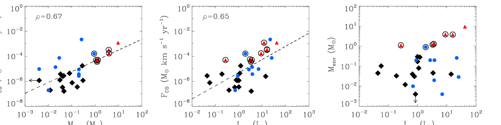
Figure 8: Correlation plots for the outflow force $F_{\rm CO}$ using M1, bolometric luminosity $L_{\rm bol}$ and the mass of the envelope $M_{\rm env}$. Black diamonds are from this study, red triangles from CB92, and blue circles from Hogerheijde et al. (1998), where $F_{\rm CO}$ was calculated by the same method as in this study. The Class 0 sources are encircled. Upper limits are indicated with arrows. The dashed line indicates the best fits to the combined data set.

In order to gain a better understanding of the outflow driving mechanism, two main trends are explored: the outflow force versus the mass of the envelope and the outflow force versus the bolometric luminosity, using the outflow force results from the $\varv_{\rm max}$ (M1) method. The envelope mass is considered an evolutionary parameter, whereas the bolometric luminosity for Class 0/I YSOs is dominated by accretion luminosity (Bontemps et al. 1996).

The correlation plots are shown in Fig. 8, where data from this study are combined with data from two other outflow studies, which used the same method (M1) for deriving the outflow force, i.e., CB92 (sample of mostly Class 0 sources) and Hogerheijde et al. (1998) (mostly Class I sources in Taurus). From the CB92 sample we have only included the low mass sources. T Tau and L1551-IRS5 appear in both CB92 and Hogerheijde et al. (1998), we have chosen to include only the latter (the values for $F_{\rm CO}$ are within a factor of 2 of each other). HH7-11 in CB92 was later classified as Class I, while L1527 IRS in Hogerheijde et al. (1998) was classified as a Class 0 source. These sources are marked accordingly in the plot. Hogerheijde et al. (1998) and CB92 measured the opacity of the line wings from ¹³CO observations and corrected for this when determining the outflow mass.

The well-known relationship between envelope mass and outflow force (Cabrit & Bertout 1992; Bontemps et al. 1996; Hogerheijde et al. 1998; Hatchell et al. 2007) is further extended with the results of this study. Envelope masses for our sample (see Table 1) were taken from Kristensen et al. (2012) where available, otherwise from van Kempen et al. (2009c). The values from Kristensen et al. (2012) are a better estimate due to full modeling of the SED using DUSTY, whereas the envelope masses from van Kempen et al. (2009c) were determined using a conversion with a single 850 $\mu$m flux. Envelope masses and classification for the CB92 and Hogerheijde sample were updated with more recent values, see Table 7. The best fit through all data points is $\log(F_{\rm CO})=(-4.4\pm 0.2)+(0.86\pm 0.19)\log(M_{\rm env})$ with Pearson’s correlation coefficient $\rho_{F_{\rm CO},M_{\rm env}}$=0.67. The relationship agrees within errors with the large range trend found by Bontemps et al. (1996). The data points from this study are offset from the other two studies, which may be due to the data used for deriving the envelope mass: the envelope masses in this study, except for Elias 29 and IRS 63, were derived from SCUBA 850 $\mu$m emission (van Kempen et al. 2009c), while Hogerheijde et al. (1998) based their envelope mass on 1.3 mm emission. The correlation coefficient is the same as was found by Bontemps et al. (1996), who uses the annulus method (M6) and a constant inclination correction, confirming our previous statement that the choice of method introduces small scatter in the values for the outflow force, but no significant changes over a large range. The decline of outflow force with envelope mass may reflect a decrease of the outflow force with evolution (Bontemps et al. 1996; Saraceno et al. 1996), but since the current envelope mass reflects both age and initial core mass, the range of envelope masses in this sample could also represent different initial conditions (Hatchell et al. 2007), so the link with evolution is less obvious.

A second well-known relationship is between outflow force and bolometric luminosity, given in the middle panel of Fig. 8. Bolometric luminosities for our sample (see Table 1) were taken from Kristensen et al. (2012) where available, otherwise from van Kempen et al. (2009c). The values from Kristensen et al. are better constrained due to the inclusion of Herschel PACS far-infrared data. The best fit through the combined data points is $\log(F_{\rm CO})=(-5.3\pm 0.2)+(1.1\pm 0.2)\log(L_{\rm bol})$ with $\rho_{F_{\rm CO},L_{\rm bol}}$=0.65. The correlation with luminosity is usually interpreted as evidence that the driving mechanism for molecular outflows is directly related to the accretion process, since the bolometric luminosity of low-mass YSOs is thought to be dominated by accretion luminosity (Lada 1985; Yorke et al. 1995). It is widely thought that outflows are momentum-driven by a jet or wind originating from the inner disk or protostar (Bontemps et al. 1996; Downes & Cabrit 2007). The most plausible energy source for this jet or wind is the gravitational energy released by accretion onto the protostar (Bontemps et al. 1996). Accordingly, the outflow force is directly related to the accretion rate $\dot{M}_{\rm acc}$. Bontemps et al. (1996) found a decline of outflow force between Class 0 and Class I, which has been taken as evidence that outflow force declines with age. In our combined sample the Class 0 sources are also offset from the Class I sources and fitting these two classes separately results in a significant change in offset ($-$5.6 vs $-$4.2, $\pm$0.2) for Class I vs 0). However, due to the selection of the older samples (the brightest outflow sources available) and the differences in data quality and derivation of parameters, the combined sample is probably not representative of the general properties of Class 0 and Class I sources.

The envelope mass as function of bolometric luminosity has been considered as an evolutionary diagram (Saraceno et al. 1996) since the parameters are correlated, but Bontemps et al. (1996) concluded that Class 0 sources do not follow the correlation and the diagram can only show the range of evolutionary stages of the sample. For our sample these two parameters only have a $\rho_{M_{\rm env},L_{\rm bol}}$ of 0.34 in combination with other studies (see right panel of Fig. 8) so their correlations with $F_{\rm CO}$ are independent. The similar correlation coefficients for these two relations have 3$\sigma$ confidentiality levels considering the sample size (Marseille et al. 2010) so we consider the correlations to be strong.

In summary, the correlation plots agree well with previous studies of the outflow force, but a decline in evolution between Class 0 and I objects is neither confirmed or ruled out.

5.3 Outflow direction

For the L1688 part of Ophiuchus, we compare the outflow directions for the different sources using Fig. 1. Since these sources are clustered together, they may have experienced the same trigger from the same direction for the core or filament formation and the following star formation. For L1688, the orientation can be divided in three groups: IRAS 16253–2429, IRS 54, IRS 37, WL 6, IRS 44 and IRS 46 are all oriented in a north-east, south-west direction. We may even add U3 (near IRS 37) and U5 (near IRS 44) to this sample, which are well enough covered to derive their orientation. The second group contains the sources with a north-west, south-east direction: Elias 29, Elias 33, VLA 1623, WL 12 and WL 17. LFAM 26 and IRS 43 do not belong to either group. The direction of the first group agrees with the results of Anathpindika & Whitworth (2008), who concluded that the outflow direction is perpendicular to the filament direction in 72$\%$ of cases. The implication is that angular momentum is delivered to a core forming in a filament, since the angular momentum will eventually drive the outflow. The Ophiuchus ridge in the south is indeed perpendicular to the outflow direction of the first group. A detailed study of filament velocities, such as performed for L1517 (Hacar & Tafalla 2011) suggesting core formation in two steps, could provide a better understanding of this phenomenon.

The distribution of outflows over two groups with an approximately equal direction suggests that there have been two separate triggering events causing the star formation or two separate filaments. Considering the large values for $L_{\rm bol}$ and $M_{\rm env}$ for the second, northern group compared to the first, southern group (mean of 3.9 $L_{\odot}$ and 0.36 $M_{\odot}$ versus 0.6 $L_{\odot}$ and 0.044 $M_{\odot}$) these two groups may have started star formation at different times, due to different events. This is consistent with the observation of Zhang & Wang (2009) that the star formation in Ophiuchus first took place in the denser northwestern L1689 region. It is further consistent with the suggestion that star formation in Ophiuchus was triggered by ionization fronts and winds from the Upper Scorpius OB association, located to the west of the Ophiuchus cloud (Blaauw 1991; Preibisch & Zinnecker 1999; Nutter et al. 2006).

6 Conclusions

We have searched for molecular outflows towards Class I sources in Ophiuchus using new high $S/N$ JCMT ¹²CO $J$=3–2 maps and compared various analysis methods for the outflow force and assumptions that go into the calculation. The main results of this study are the following:

1. All embedded sources classified as ‘Stage 1’ by van Kempen et al. (2009c) show bipolar outflow activity, except for those that are so close to another source that their outflows are confused. Five new outflows are detected. These results are consistent with the fact that every embedded source likely has a bipolar outflow. The methods used for determining integration limits and deriving physical properties strongly influence the results of outflow studies, but for large data sets over broad ranges of $L_{\rm bol}$ and $M_{\rm env}$ the trends are still similar. For weak outflows and clustered star formation, detailed analysis and high resolution observations are crucial.

2. Seven different analysis methods for deriving the outflow force are analytically described and applied to all Ophiuchus sources in the sample, plus the well-studied sources HH 46 and NGC1333 IRAS 4A. All methods agree with each other within a factor 6. The methods that do not involve inclination correction factors give lower values for the outflow force for the largest inclination angle by a factor 2–3, but no other systematic effects related to inclination exist. Although the true outflow force remains unknown, the separation method (separate calculation of dynamical time and momentum) is least affected by the uncertain observational parameters.

3. The effect of subtraction of an off-source spectrum, representative of an envelope profile, is studied. After this subtraction, the outflow material at ambient velocities, blended in with the envelope material can be measured. It is found that including ambient material does not increase the outflow force by more than a factor of 5 and generally much less.

4. The outflow force remains constant as a function of radius, so the outflow force can be analyzed with partial coverage CO maps as long as it is centered on the source position.

5. Observational properties and choices in the analysis procedure can individually affect the outflow force up to a factor of a few. The most important factor to consider is the $S/N$ of the data: a strong dependence of the outflow force on the noise level means that the methods described cannot always be applied directly.

6. When combining the results from different studies, using different methods, assumptions and/or data quality, scatter up to a factor of 5 can be expected. Discrepancies in derived outflow force between different studies are up to an order of magnitude and can be explained by comparing the analysis methods.

7. Comparing the outflow observations for three sources with recently obtained disk studies (Jørgensen et al. 2009) leads to revision of these disk structures. IRS 63 shows an excellent agreement for the disk orientation (perpendicular to the outflow direction), but for Elias 29 the assumed disk emission most likely originates from the outflow material itself, close to the source, consistent with a non-detection in millimetre continuum at long baselines. IRS 43 is even more complex: the outflow direction was found to be pole-on, which is completely inconsistent with the previously identified edge-on disk orientation.

8. The well-known correlations of outflow force with envelope mass and bolometric luminosity are extended with the results of this study, confirming a direct correlation of outflow strength with both properties.

9. The outflows in the L1688 region can be divided into two groups, based on preferred outflow direction and significantly different evolutionary properties. This suggests a scenario with star formation in two separately triggered events, starting in the north west, supporting conclusions from previous work, e.g. Zhang & Wang (2009).

For further outflow studies, it is important to consider the choice of methods and assumptions that go into the calculations, especially when comparing with previous results. For Ophiuchus, a complete map of the entire L1688 region in low-$J$ CO lines, as recently performed for Perseus (Curtis et al. 2010), would provide a more complete view of outflow activity, both for known as well as for new sources (such as the Us) and a more complete view of outflows from Stage 2 sources. Furthermore, the envelope surrounding IRS 43 should be explored in very high spatial resolution in order to understand the complex velocity structure. Limitations by single dish observations will be solved further using the Atacama Large Millimeter Array (ALMA).

Appendix A Newly discovered outflows

From detailed spectral analysis, new bipolar outflow structures were discovered in several CO maps, not belonging to any of the sources in the embedded source sample of van Kempen et al. (2009c). In this section we look for other suitable candidates of embedded sources. The partial coverage of these outflows extends the field in which to look for a candidate.

• The outflow structure U1 south west of IRS 63 may originate from the submillimeter core SMM J 163133–24032, which was matched by Jørgensen et al. (2008) with the Spitzer YSO candidate SSTc2d J163134.29-240325.2 (Evans et al. 2009), located 24$\arcsec$ away, classified as a Class I source with $L_{\rm bol}$ = 0.88 $L_{\odot}$ and $T_{\rm bol}$ = 870 K.

• For U2, selecting a candidate is somewhat difficult, as only a small piece of the red lobe is covered and therefore the direction of the originating source is unknown. The most likely candidate is the submillimeter core SMM J 163143–24003 (Jørgensen et al. 2008) at 2.2$\arcmin$ north east of IRS 63 (see Fig. 9) with a dust temperature of 15 K. No infrared source is known near this location.

• U3 is located to the west of IRS 37. The elongated structure and direction of the outflow suggest that the powering source is located to the south west. The large submillimeter core SMM J162713–24295 (Jørgensen et al. 2008) is a likely candidate (see Fig. 9) with a dust temperature of 18 K. The shape of this submillimeter core is consistent with the outflow direction, which is usually perpendicular to the ridge (Anathpindika & Whitworth 2008). Again, no infrared source is known at this location.

  

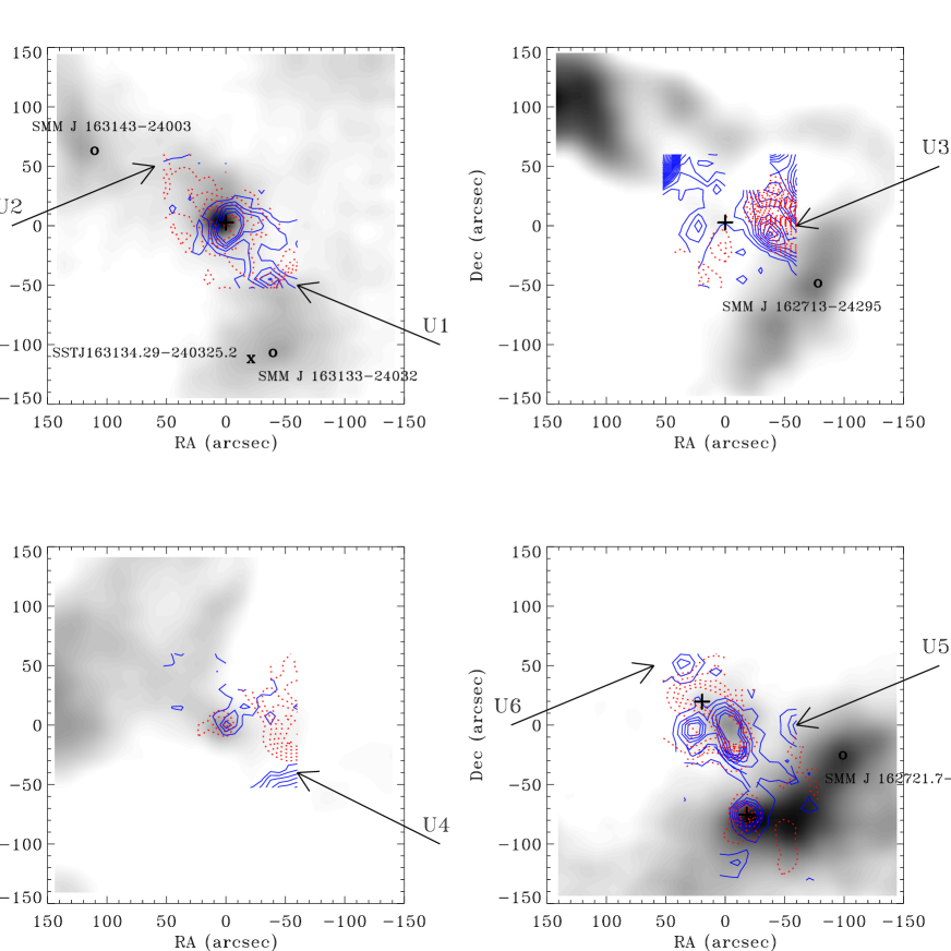
  Figure 9: The regions around the new outflow structures (Us), showing the SCUBA 850 $\mu$m emission in the background, the contour map of the integrated line wings, the sources from the sample in this study marked with pluses and the Us indicated with arrows. The nearby submillimeter cores are marked with circles and infrared sources with a cross. (Top left) The region around IRS 63. (Top right) The region around IRS 37. (Bottom left) The region around WL 12. (Bottom right) The region around IRS 44.

• The outflow U4 is clearly visible in the WL 12 map (Fig. 9). The center of origin is about 16:26:40, -24:35:27. There are no submillimeter cores or infrared sources nearby. Estimates of a SED or $T_{\rm bol}$ are therefore not possible at this time.

• U5 is located to the west of IRS 44 (Fig. 9). Towards the south-west is submillimeter core J162721.7-244002, (Di Francesco et al. 2008), which is a possible candidate for the powering source. However, just like U3, there is no infrared source at this position. No temperature was derived for this core, but the 450 and 850 $\mu$m fluxes in combination with the non-detection at 70 $\mu$m and shorter wavelengths indicate a very low dust temperature between 5 and 10 K.

• Only the blue lobe of U6 is detected, but there are no submillimeter cores or infrared sources nearby. Estimates of a SED or $T_{\rm bol}$ are therefore not possible at this time.

The Us are clearly peculiar objects. Only U1 could be assigned to a YSO candidate, a submillimeter core with an infrared detection. U2, U3 and U5 are interesting since they have a possible source of origin in submillimeter cores without infrared detection, suggesting either a very low temperature and luminosity, a very deeply embedded object, an edge on geometry or a new kind of object, producing an outflow or some other mechanism producing swept-up gas. For U4 and U6 not even a submillimeter core was detected. U2, U5 and U6 are only marginally covered and therefore possibly no new outflows: they may be part of the main outflow in the map and only seem separate due to density variations in the envelope. However, for U1, U3 and U4 this is not very likely considering their morphology. Full spatial coverage of low-$J$ CO lines of these regions may provide an answer. Far-infrared fluxes provided by Herschel may help to define the cold cores (Bontemps et al. 2010, e.g.) and derive their properties, to conclude whether they can be the powering sources of these outflows.

Appendix B Comparison with other outflow studies

Table 5: Comparison of the outflow force between this study and other outflow studies.

Source	$F_{\rm CO}$	$F_{\rm CO}$	References
	(10${}^{-6}M_{\odot}$ km s-1 yr-1)
WL 12	0.12	6.0	1
LFAM 26	2.0	16,4.7	2,3
WL 17	0.25	…	…
Elias 29	1.9	15,9.8,14.5,2.0	1,2,3,4
IRS 37	0.14	…	…
WL 6	0.9	$<$15,2.5	1,4
IRS 43	0.26	15	1
IRS 44	3.2	27,3.4	1,4
IRS 46	2.8	…	…
Elias 32,33	13.44	9.6,146	3,5
IRS 54	0.9	…	…
IRAS 16253–2429	0.57	1
IRS 63	0.9	6.3	1

(1) Bontemps et al. (1996), (2) Bussmann et al. (2007), (3) Nakamura et al. (2011), (4) Sekimoto et al. (1997), (5) Kamazaki et al. (2003)

Table 6: Comparison of the methods and observation properties between this study and other outflow studies.

	This study	Bontemps et al. (1996)	Sekimoto et al. (1997)
12CO line	3–2	2–1	2–1; 1–0
Sources	All	EL 29, IRS 43, IRS 44, WL 6, WL 12	EL 29, IRS 44, WL 6
Beam size ($\arcsec$)	15	30(NRAO), 10(IRAM)	34
Map size ($\arcsec\times\arcsec$)	120$\times$120	60x60(NRAO), 25x25(IRAM)	68$\times$68
Velocity res. (km/s)	0.1	0.65(NRAO), 0.26(IRAM)	0.06; 0.05
$\sigma_{\rm rms}$ (K)	0.15	0.25(NRAO), 0.15(IRAM)	0.2; 0.15
Method	$\varv_{\rm max}$ (M1)	annulus (M6)	$\varv_{\rm max}$ (M1)
$\varv_{\rm in}$	off-source	$T_{\rm peak}/10$	unknown
$\varv_{\rm out}$	1$\sigma$ cut-off	1$\sigma$ cut-off	unknown
Opacity corr.	none	mean of CB92: 3.5	derived from 13CO: $\sim$3.0(2–1)
Inclination corr.	factors CB92	average $i$=57.3: factor 2.9	factors CB92
Distance to Oph (pc)	120	160	160
Other		Average off-source spectrum subtracted
		before integration, integration
		radius 45$\arcsec$(IRS 44), 15$\arcsec$(others)

	Kamazaki et al. (2003)	Bussmann et al. (2007)	Nakamura et al. (2011)
12CO line	3–2	3–2	3–2
Sourcesa	Elias 32/33	EL 29, LFAM 26	Elias 29,Elias 32/33,LFAM 26
Beam size ($\arcsec$)	14	11	40
Map size ($\arcsec\times\arcsec$)	$120\times 240$ (OphB2)	$300\times 300$	$23\arcmin\times 23\arcmin$
Velocity res. (km/s)	0.33	0.4	0.4
$\sigma_{\rm rms}$ (K)	0.79 (OphB2)	0.4	0.28
Method	$\langle\varv\rangle$ (M3)	$\varv_{\rm max}$ (M1)	$\varv_{\rm max}$ (M1)
$\varv_{\rm in}$	channel maps	unknown	channel maps
$\varv_{\rm out}$	3$\sigma$ cut-off	unknown	3$\sigma$ cut-off
Opacity corr.	5.4	none	none
Inclination corr.	average $i$=57.3: factor 2.9	none	$\frac{\sin i}{\cos i}$, $i$=80 (El 29, LFAM 26), $i$=57.3 (El 32)
Distance to Oph (pc)	160	120	125
Other

Of our sample of 16 sources, 11 sources were studied previously (Bontemps et al. 1996; Sekimoto et al. 1997; Kamazaki et al. 2003; Bussmann et al. 2007; Nakamura et al. 2011) but often with different derived properties. We compare the results, methods and available observations in Table 5 and 6.

The sources studied by Bontemps et al. (1996) have a systematic offset in $F_{\rm CO}$ due to their opacity correction of 3.5. If this factor is removed, their outflow forces are still typically a factor of 2 higher if we use the same annulus method (M6) on our data set (see Fig. 5). Since their rms level is similar to our study and other effects due to coverage or method can be excluded, the only other explanation may be the determination of the inner velocity limit: Bontemps et al. used $T_{\rm peak}/10$ for $\varv_{\rm in}$, but $T_{\rm peak}$ is source dependent and easily affected by the presence of foreground clouds. When the inner velocity limit is moved 1 km s^-1 inwards, the outflow force is increased by a factor of 2 (see Fig. 10). The inclination factor of 2.9 for a constant $i=57\degr$ does not cause significant underestimates, since none of these five sources have an inclination of 70$\degr$ which generally requires a larger correction factor (see Fig. 5).

The values found by Sekimoto et al. (1997) agree very well (within a factor of 1.8) with the results in this study, as expected considering their methods and data quality. However, they derived an opacity in the line wings from ¹³CO lines of 3.0 for the 2–1 lines, similar to CB92. The results for LFAM 26 and Elias 29 in the study from Bussmann et al. (2007) are both a factor of $\sim$5 higher. Inspection of the individual parameters shows that this difference is dominated by the effect of integrated mass, which is more than 10 times larger in their study, whereas their dynamical time is only twice as long compared to our results. The observations presented by Bussmann et al. cover the entire outflow of Elias 29 and LFAM 26. Apparently the mass is not uniformly spread over the outflow lobes, so the outflow momentum may not be conserved along the lobe in this case.

The outflow force for Elias 33 also agrees well with the value found by Kamazaki et al. (2003), considering their opacity correction of 5.4. Considering their high rms level and 3$\sigma$ cut-off, their derived outflow velocities are only 5.6 and 3.6 km s^-1, for the blue and red lobe, respectively, versus 12.0 and 10.0 km s^-1 in this study. This would decrease the outflow force with a factor of 4–5, but this is compensated by the total (uncorrected) mass derived by Kamazaki et al.  which is more than 5 times larger than derived in this study.

Our results do not match well with the results from Nakamura et al. (2011): LFAM 26 is comparable, but our value for Elias 29 is 7 times smaller while the value for Elias 32/33 is 2 times larger. The reason for this discrepancy may be the choice of inclination angles: the adopted value of 80$\degr$ for Elias 29 and LFAM 26 with the projection formula ${\sin i}/{\cos i}$ used by Nakamura results in a correction factor of 6, the adopted value of 57$\degr$ for Elias 32/33 gives a correction of 1.6, while in this study an inclination of $50\degr$ was assumed for Elias 29 (correction factor 0.45) and $i=70\degr$ for Elias 32/33 (correction factor 1.6). The 3$\sigma$ cutoff and low $S/N$ data used by Nakamura et al. would have resulted in lower values of the outflow force for all three sources with a factor 2–4, but this is counterbalanced by the use of larger correction factors (6 versus 1.1 and 1.6 versus 0.45).

This section shows again that, in order to compare and combine outflow studies, similar methods have to be applied, since results from the studies discussed can differ by more than one order of magnitude. Since opacity and inclination cause the largest variations in the outflow force, it is essential to derive these properties as accurately as possible.

Appendix C Mass derivation

The main physical parameters of the outflow are the mass, $M$, the velocity, $\varv_{\rm CO}$ (defined as $|\varv_{\rm out}-\varv_{\rm source}|$), and the projected size of the lobe $R_{\rm lobe}$, for both the blue and red lobe. The mass is calculated from the column density assuming an excitation temperature of 100 K (e.g. Yıldız et al. 2012). The column density of the ¹²CO upper level $u$ (in this case $J$=3) is derived from the integrated intensity of the line wings as follows.

$$N_{\rm u}=\frac{8\pi k\nu^{2}\int T_{\rm mb}(\varv)\mathrm{d}\varv}{hc^{3}A_{\rm ul}}$$ (10)

The column density of the upper level, $N_{\rm u}$ (cm^-2), is converted to ${\rm H}_{2}$ column density $N$ by

$$N=N_{\rm u}\times\left[\frac{{\rm H}_{2}}{{}^{12}{\rm CO}}\right]Q(T)[g_{\rm u}e^{-E_{\rm u}/kT}]^{-1}\\$$ (11)

with $Q(T)$ the partition function and using ${\rm H}_{2}/^{12}{\rm CO}=1.2\times 10^{4}$ (Frerking et al. 1982) and $N$ is converted to mass in grams using

$$M=\mu m_{H}A\times N$$ (12)

with a mean molecular weight $\mu$ of 2.8 used to include He (Kauffmann et al. 2008) and $A$ the physical area covered by one pixel. Summarizing, the conversion from integrated intensity to mass is a multiplication with constant $K$:

$$K=\mu m_{H}A\times\left[\frac{{\rm H}_{2}}{{}^{12}{\rm CO}}\right]Q(T)[g_{\rm u}e^{-E_{\rm u}/kT}]^{-1}\frac{8\pi k\nu^{2}}{hc^{3}A_{\rm ul}}$$ (13)

With these basic physical quantities, a number of outflow parameters can be derived: the momentum, $p$, the dynamical age, $t_{\rm d}$, the mass outflow rate, $\dot{M}$ and the outflow force, $F_{\rm CO}$. The basic equations are:

$$p = M\varv_{\rm CO}$$ (14)

$$t_{\rm d} = \frac{R_{\rm lobe}}{\varv_{\rm CO}}$$ (15)

$$\dot{M} = \frac{M}{t_{\rm d}}$$ (16)

$$F_{\rm CO} = \frac{M\varv_{\rm CO}^{2}}{R_{\rm lobe}}=\frac{p}{t_{\rm d}}$$ (17)

The velocity, $\varv_{\rm CO}$, often called $\varv_{\rm max}$, is not a well-constrained parameter: due to the inclination and the shape of the outflow, often following a bow shock including forward and transverse motion, the measured velocities along the line of sight are not necessarily representative of the real velocities driving the outflow (Cabrit & Bertout 1992). This is the main reason why various methods have been developed to derive the outflow force, where a correction factor is often applied to compensate for these effects.

Appendix D Influence of assumptions and data quality

Apart from the analysis method, a number of choices, observational properties and assumptions may influence the value of the outflow force. The effects are tested using the $\varv_{\rm max}$ method (M1) on a small sample of four targets: Elias 29, IRS 54, HH 46 and IRAS 4A. The results are presented in Fig. 10. In each plot, the resulting outflow force is normalized to the ‘standard’ value, which is the outflow force resulting from the best estimate of that parameter using the recipe in Sect. 4.2.

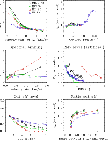
Figure 10: Influence of observational properties and choices on the resulting value of the outflow force, using M1 ($\varv_{\rm max}$) on Elias 29, IRS 54, HH 46 and IRAS 4A, which all have clear, isolated outflows. See text for description of each category. It follows that these observational properties and choices in the analysis procedure affect the outflow force up to a factor of 4–5.

D.0.1 Inner velocity limits

The inner velocity limits are determined from the width of the (averaged) off-source spectra. In general, it can be difficult to determine where the outflow emission blends in with the ambient envelope emission (see also Sect. 4.3). The first panel shows how the outflow force changes if the inner velocity limits are shifted simultaneously inwards (negative) or outwards (positive), relative to the best guess based on off-source emission. When the inner limits are moved inwards, more and more integrated emission is taken into account, also including more envelope emission, increasing the mass of the outflow up to a factor of 5, but certainly within 0.5 km s^-1 the significance remains within a factor of 2. Moving the limits outwards decreases the outflow force by a factor of 2. For IRAS 4A, the outflow force increases only slightly moving inwards: due to the high velocities involved, the integrated mass is not the dominant parameter. For the intensity-weighted methods the change of the inner velocity limit changes the outflow force even less since the intensity at low velocities does not contribute much to the total outflow force.

D.0.2 Spatial coverage

Bontemps et al. (1996) suggested that it does not matter how much of the outflow emission is spatially covered for calculating the outflow force, as long as the correct size $R_{\rm lobe}$ is taken for the spatially covered spectra, because the momentum is conserved along the outflow lobes. To test this assumption, a range of radii were chosen starting at the central position in each map and finishing at the border of the map. When taking a larger radius, more and more spectra are integrated, but $R_{\rm lobe}$ simultaneously increases. Nearby outflows from other sources are excluded beforehand. Panel 2 in Fig. 10 shows that the outflow force indeed remains constant as a function of radius. The outflow force of IRAS 4A increases significantly up to a factor 3 due to the inclusion of a “bullet” and high-velocity emission starting around 90$\arcsec$. Elias 29 decreases slightly at larger radii, due to the two broken receivers as shown in Fig. 3, where parts of the lobes are missing. This figure proves that the outflow force can be analyzed with partial coverage as long as it is centered on the source position, but one has to be careful with emission from other sources, “bullet” emission and when regions of data are missing.

D.0.3 Spectral binning

Astronomical spectra are often rebinned to lower spectral resolution in order to decrease the rms, since lines of outflows have broad spectral profiles. When the outflow velocity limits are based on the rms level, binning to larger bin sizes may influence the outflow force significantly. This is investigated in panel 3 in Fig. 10. The outflow force remains constant within a factor of 2 for Elias 29, IRS 54 and IRAS 4A. Inspection of the mass as function of bin size (not shown here) shows a decrease of the integrated mass, but this is apparently compensated by the higher outer velocities. On the other hand, HH 46 shows a significant increase of outflow force. This is due to the low $S/N$ of this data set: the lower rms moves $\varv_{\rm max}$ rapidly outwards while the inner velocity remains almost constant. Therefore, one has to be careful with binning spectra when using an rms cut-off for the velocities, since the choice of binning may further increase the outflow force significantly. The intensity-weighted methods, such as M7, are less affected by rebinning.

D.0.4 Cut-off level

The rms level determines the outer velocity and therefore the outflow force depends on the quality of the data. In order to investigate this, the observed high quality spectra are convolved with an artificial noise signal and the velocity limits are redetermined with the new rms. The resulting outflow force as function of new rms is shown in panel 4 of Fig. 10: the outflow force can be underestimated by a factor of 5–10 for large noise levels ($S/N<5$ for the wing emission). The outflow force of HH 46, which already has a large noise level to start with, is likely to be underestimated.

In some studies, the rms cut-off is not taken at 1$\sigma$, but rather 3$\sigma$ or even 10$\sigma$ to determine the outer velocities. The effect of taking a cut-off at multiple $\sigma$ is investigated in panel 5. The outflow force decreases slowly when taking a stricter cut-off but the overall effect remains within a factor of 3-4, except for the spectra of HH 46 with low $S/N$.

D.0.5 $\varv_{\rm out}$: ratio cut-off

Due to the disadvantages of using an rms cut-off described above, another method is sometimes applied. The cut-off limit is defined as e.g. 1% of the intensity at the inner velocity limit of the outflow wing (DC07). In that case, the cut-off level depends on the brightness of the source itself, rather than the quality of the observations. The difference between these two methods is investigated in Panel 6 of Fig. 10, where the outflow force is normalized to the value found by the rms cut-off. The outflow force is likely to be underestimated for a ratio smaller than 50. For the larger ratios, the outflow force remains constant, which means that the outflow wing is sufficiently steep: the outer velocity is not affected by this small change in the cut-off level.

D.0.6 Summary

Observational properties and choices in the analysis procedure can affect the outflow force up to a factor of 4–5. Small changes in the inner velocity limit, the rms level, the cut-off significance and binning do not change the outflow force more than a factor of 2. It is demonstrated that the spatial coverage in principle does not influence the outflow force, indicating that this is a conserved quantity. Also, choosing a percentage of the emission at the inner velocity limit for the cut-off does not in principle change the outflow force, as long as the percentage is small enough. The most important factor to consider is the $S/N$, as shown in the results of HH 46 with a higher noise level. A strong dependence of the outflow force on the noise level (Fig. 10) implies that the methods described cannot always be applied directly. When combining the results from different studies, using different methods, assumptions and/or data quality, scatter up to a factor of 5 can be expected.

Appendix E Outflow parameters from other studies

Table 7: Outflow and evolutionary parameters from other studies used in evolutionary trends.

Name	Class	$F_{\rm CO}$	Ref. ($F_{\rm CO}$)	$L_{\rm bol}$	$M_{\rm env}$	Ref. ($L_{\rm bol}$,$M_{\rm env}$)
		($M_{\odot}$ km s-1		($L_{\odot}$)	(10${}^{-2}M_{\odot}$)
		yr-1)
L1448-C	0	1.7($-$4)	1	9.0	390	2
L1455M-FIR	0	3.5($-$4)	1	16	-	1
HH7-11	I	1.2($-$3)	1	41.8	950	2
IRAS3282	0	5.6($-$3)	1	3.0	-	1
RNO43-FIR	0	1.2($-$3)	1	12	-	1
VLA1623	0	5.0($-$5)	1	0.27	111	3
IRAS16293	0	3.2($-$4)	1	16	3.8	4,5
L723	0	5.0($-$5)	1	3.6	130	2
B335	0	3.6($-$5)	1	3.3	120	2
L1489 IRS	I	1.4($-$5)	6	3.7	2.0	6
T Tau	I	7.3($-$5)	6	25.5	2.9	6
Haro 6-10	I	9.4($-$6)	6	6.98	0.40	6
L1551 IRS5	I	2.2($-$3)	6	21.9	26	6
L1535 IRS	I	1.9($-$7)	6	0.70	10	6
TMR 1	I	3.7($-$6)	6	3.8	20	2
TMC 1A	I	8.7($-$6)	6	2.7	20	2
L1527 IRS	0	1.6($-$4)	6	1.9	90	2
TMC 1	I	2.6($-$6)	6	0.9	20	2
Ced110IRS4	I	4.6($-$5)	7	0.8	20	2
CrAIRAS32	I	1.8($-$4)	7	3.4	80	7
HH100	I	$<$5.3($-$3)	7	17.7	810	2
RCrAIRS7	I	$<$4.9($-$2)	7	20	630	7

(1) CB92, (2) Kristensen et al. (2012), (3) van Kempen et al. (2009c), (4) Evans et al. (2009), (5) Jørgensen et al. (2008), (6) Hogerheijde et al. (1998), (7) van Kempen et al. (2009b)

Appendix F Spectra overview

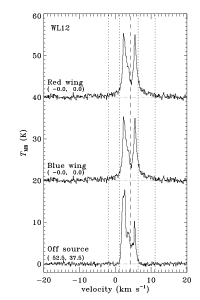
(a)

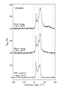
(b)

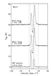
(c)

Overview of relevant outflow spectra. Each diagram shows from top to bottom the strongest red wing spectrum, the strongest blue wing spectrum and an off-source spectrum. $\varv_{\rm source}$ (dashed line) and the integration limits (dotted lines) are indicated. A dash-dotted line indicates the baseline. Positions of each spectrum are indicated in parentheses.

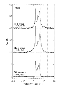
(d)

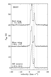
(e)

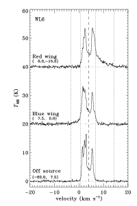
(f)

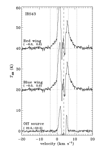
(g)

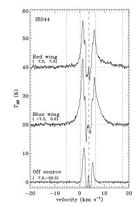
(h)

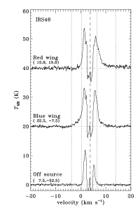
(i)

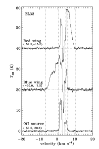
(j)

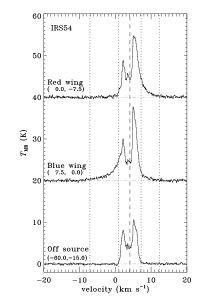
(k)

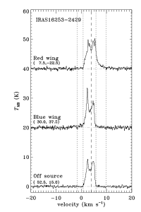
(l)

Overview of relevant outflow spectra - Continued

Table 8: Integration limits of the ¹²CO $J$=3–2 line wings.

		Blue lobe		Red lobe
Name	$\varv_{\rm source}$	$\varv_{\rm out}$	$\varv_{\rm in}$	$\varv_{\rm out}$	$\varv_{\rm in}$
	(km s-1)	(km s-1)	(km s-1)	(km s-1)	(km s-1)
WL 12	4.3	-1.8	1.2	6.3	11.1
LFAM 26	4.2	-0.7	1.0	6.7	11.5
LFAM 26	4.2	-1.0	1.0	7.0	17.0
WL 17	4.5	-0.5	1.0	6.0	9.8
EL 29	4.6	-5.2	1.4	7.0	13.4
IRS 37	4.2	-2.0	0.5	5.7	8.1
WL 6	4.0	-3.3	0.5	6.7	14.3
IRS 43	3.8	-3.9	0.1	6.3	11.1
IRS 44	3.8	-5.2	0.4	6.5	17.5
IRS 46	3.8	-3.7	0.4	6.5	14.1
EL 33	4.5	-6.7	0.8	6.0	10.3
IRS 54	4.1	-7.1	1.0	7.2	12.4
IRAS 16253-2429	4.0	-1.6	0.7	5.8	9.8
IRS 63	2.7	-7.3	1.6	3.8	7.3
U1	2.7	-2.2	1.6	3.8	7.3
U2	2.7	0.0	1.6	3.8	6.0
U3	4.2	-4.6	0.5	5.7	9.0
U4	4.3	-0.3	1.2	6.3	9.0
U5	3.8	-2.4	0.4	6.5	9.8
U6	3.8	-2.6	0.4	6.5	8.6