Bistable generalised Langevin dynamics driven by correlated noise possessing a long jump distribution: barrier crossing and stochastic resonance

Abstract

The generalised Langevin equation with a retarded friction and a double-well potential is solved. The random force is modelled by a multiplicative noise with long jumps. Probability density distributions converge with time to a distribution similar to a Gaussian but tails have a power-law form. Dependence of the mean first passage time on model parameters is discussed. Properties of the stochastic resonance, emerging as a peak in the plot of the spectral amplification against the temperature, are discussed for various sets of the model parameters. The amplification rises with the memory and is largest for the cases corresponding to the large passage time.

I Introduction

The stochastic dynamics may not always be restricted to familiar problems involving Gaussian distributions. In realistic systems long jumps are frequently observed and the variance may be infinite, as it is the case for the general Lévy stable distributions which possess power-law tails. Since a medium nonhomogeneity is typical for systems exhibiting long jumps, one can expect that a random force in a dynamical description of those systems depends on the process value, i.e. the stochastic equation contains a multiplicative noise. An interesting property of such description is a possibility that the variance acquires a finite value even if the underlying process is assumed as a non-Gaussian Lévy stable process, defined by the stability index $\alpha$ $(0<\alpha<2)$ sro09 .

The covariance functions are finite as well. The autocorrelation function for the generalised Ornstein- Uhlenbeck process $\xi(t)$, defined by the Langevin equation driven by a multiplicative Cauchy noise, falls with time like a stretched exponential but may be reasonable approximated by a simple exponential sron . Then the process $\xi(t)$ comprises two features: it exhibits long jumps and possesses well-defined covariance functions. When such a process enters a stochastic equation as a random driving, the finite correlation time requires a usual damping term to be substituted by a retarded friction to ensure a proper equilibrium state. This problem is well-known for the Gaussian processes: one can construct an effective low-dimensional equation describing a many-body system in which individual variables are coupled by harmonic oscillators mori . The effective equation – the generalised Langevin equation (GLE) – is non-local in time and satisfies the fluctuation-dissipation theorem kubo . Moreover, the effective random force is Gaussially distributed. If velocities of bath particles are non-Gaussian but of finite variance, one may still expect convergence to the Gaussian, according to the central limit theorem. However, this theorem does not apply in the presence of long range correlations, which is natural in complex systems. On the other hand, large higher moments make convergence to the Gaussian impossible even if independent variables are linearly combined. In particular, the distance of that distribution from the Gaussian is infinite when the third moment diverges, according to the Berry-Esséen theorem fel . Therefore, the effective noise may be non-Gaussian and the dynamics of such systems may still be described by GLE cof . GLE driven by $\xi(t)$ for the case without a deterministic force was analysed in Ref.sron . The probability density distributions converge with time to a stationary state with a power-law tail; the variance grows linearly with time indicating a normal diffusion.

In this paper, we consider GLE driven by $\xi(t)$ for the case of a bistable system and activated, in addition, by a periodic force. We address a physically important problem of the time characteristics of the barrier penetration and analyse the influence of the memory on this process. We calculate, in particular, the mean first passage time (MFPT) as a function of model parameters. When the rate of the jumping between the potential wells due to the noise coincides with the frequency of the oscillatory force, the stochastic resonance (SR) is observed. We discuss this phenomenon and demonstrate how model parameters modify its properties, in particular the position and intensity.

II Stochastic equations and density distributions

The ordinary Ornstein-Uhlenbeck process describes motion of the particle subjected to a linear deterministic force and an additive Gaussian white noise. It can be generalised by admitting a dependence of the noise on the process value (a multiplicative noise) and including non-Gaussian distributions, in particular the Lévy stable distributions with power-law tails. Then the generalised process obeys the following Langevin equation

$$\dot{\xi}(t)=-\gamma\xi(t)+G(\xi)L(t),$$ (1)

where $L(t)$ is the noise and a given function $G(\xi)$ may be responsible e.g. for a nonhomogeneous structure of the environment. Since $L(t)$ is a white noise, Eq.(1) is not unique and requires a clarification at which time $G(\xi)$ is to be evaluated; in the following the Stratonovich interpretation will be applied. We assume

$$G(\xi)=K|\xi|^{-\theta},$$ (2)

where the constant $K$ has the dimension $[K]=$cm^θ. The algebraic form of Eq.(2) is well suited to describe e.g. self-similar systems. Moreover, distribution of the independent increments of $L(t)$ is assumed in a form of the symmetric Cauchy distribution,

$$p_{C}(x)=\frac{1}{\pi}\frac{D}{D^{2}+x^{2}},$$ (3)

where a generalised diffusion coefficient $D$ has the dimension $[D]=$ cm/sec. All moments of the distribution (3) are infinite. In the Stratonovich interpretation, a distribution corresponding to Eq.(1) can be easily derived by introducing a new variable,

$$\eta=\frac{K^{-1}}{1+\theta}|\xi|^{1+\theta}\hbox{sgn}(\xi),$$ (4)

which transforms Eq.(1) to an equation with the additive noise,

$$\dot{\eta}(t)=-\gamma_{\theta}\eta(t)+L(t),$$ (5)

where $\gamma_{\theta}=\gamma(1+\theta)$ sro09 . Distribution of the original variable reads

$$p_{\xi}(\xi,t)=\frac{|\xi|^{\theta}}{DK\pi\gamma_{\theta}}\frac{1-\exp(-\gamma_{\theta}t)}{\xi^{2+2\theta}/D^{2}K^{2}(1+\theta^{2})+(1-\exp(-\gamma_{\theta}t))^{2}/\gamma_{\theta}^{2}};$$ (6)

the initial condition is $p_{\xi}(\xi,0)=\delta(\xi)$. The variance exists if $\theta>1$ and it can be strictly derived sro09 . The formula for the autocorrelation function, in turn, requires an integration of the process values with the transition probability,

$${\cal C}(t)=\langle\xi(0)\xi(t)\rangle=\int\int\xi_{1}\xi_{2}p_{\xi}(\xi_{2},t;\xi_{1},0)d\xi_{1}d\xi_{2}=\int\int\xi_{1}\xi_{2}p_{\xi}(\xi_{2},t|\xi_{1},0)p_{\xi}(\xi_{1})d\xi_{1}d\xi_{2},$$ (7)

where $p_{\xi}(\xi)=\lim_{t\to\infty}p_{\xi}(\xi,t)$ and $p_{\xi}(\xi_{2},t|\xi_{1},0)$ is the conditional probability. One can prove that the asymptotic time-dependence of ${\cal C}(t)$ is exponential with the rate $\gamma$ but only if one introduces a truncation of the distribution (3). Otherwise, a numerical evaluation of the double integral (7) reveals a stretched exponential shape at large time sron . However, a deviation of ${\cal C}(t)$ from the simple exponential is very small and the dependence of the rate on both system parameters, $\gamma$ and $\theta$, appears simple. Therefore, we may approximate the covariance by the following expression,

$${\cal C}(t)=(KD)^{2/(1+\theta)}\frac{\gamma^{-2/(1+\theta)}}{\cos(\pi/(1+\theta))}\hbox{e}^{-\lambda t},$$ (8)

where $\lambda=0.80(\theta+0.31)\gamma$ follows from the numerical analysis.

We consider a dynamical system described by GLE which is driven by the process $\xi(t)$ and contains a deterministic force $F(x,t)=-\partial V(x,t)/\partial x$. Therefore, $\xi$ is now interpreted as a force with the dimension $[\xi]=\hbox{g cm/sec}^{2}$ and, accordingly, $[K]=(\hbox{g cm/sec}^{2})^{\theta}$ and $[D]=\hbox{g cm/sec}^{3}$. The equation is the following:

$$m\frac{dv(t)}{dt}=F(x,t)-m\int_{0}^{t}K(t-\tau)v(\tau)d\tau+\xi(t),$$ (9)

where $v(t)$ is a velocity and $m$ denotes the particle mass. The memory kernel is related to the noise autocorrelation function by the second fluctuation-dissipation theorem, $K(t)={\cal C}(t)/mT$, where $T$ is the temperature and the Boltzmann constant is set at one. The correlation time parameter $\lambda$ is determined not only by the damping $\gamma$, as it is the case for the ordinary Ornstein-Uhlenbeck process, but also by $\theta$. Since $1/\lambda$ is to be interpreted as the memory time, we require that ${\cal C}(t)$ converges to the delta function in the limit $\lambda\to\infty$. Therefore, we rescale the driving noise: $\xi(t)\rightarrow c_{1}\sqrt{\lambda}\xi(t)$, where $c_{1}=\sqrt{0.5411{\cal C}(0)}$ has the dimension $\sqrt{\hbox{sec}}$, and appropriately modify the kernel. Mathematically, Eq.(9) represents an integro-differential equation of the Volterra type which is nonlinear in general; it cannot be solved by an integral transforms technique and we must resort to numerical methods. GLE is easier to handle when we substitute Eq.(9) by a system of the differential equations which a procedure is possible for the exponential $C(t)$. A simple derivation yields

$$m\dot{v}(t) = F(x,t)-mw(t)+c_{1}\sqrt{\lambda}\xi(t)$$

$$\dot{w}(t) = -\lambda w(t)+c_{1}^{2}{\cal C}(0)\lambda v(t)/mT$$

$$\dot{x}(t) = v(t)$$

$$\dot{\eta}(t) = -\gamma(1+\theta)\eta(t)+L(t).$$ (10)

We assume the initial conditions: $x(0)=x_{0}$, $v(0)=v_{0}$, $w(0)=0$ and $\eta(0)$ is given by a stationary distribution for the process (5). Moreover, we assume in the numerical calculations $D=1\,\hbox{g cm/sec}^{3}$ and $K=1\,(\hbox{g cm/sec}^{2})^{\theta}$. GLE in a form similar to (II) is frequently studied for the Gaussian processes, e.g. for such problems as the transport of the Brownian particles lucz1 ; lucz , non-Markovian features of the nonlinear GLE far and a fractional superdiffusion sie . In those cases the system (II) represents an equivalent Markovian dynamics in a higher-dimensional space which may be expressed by a multidimensional Fokker-Planck equation. The present case is more complicated, even in the absence of the potential, because of the non-linear relation between $\eta$ and $\xi$, Eq.(4).

First, let us consider a time-independent bistable potential,

$$V(x)=-\frac{A}{2}x^{2}+\frac{B}{4}x^{4},$$ (11)

which has two minima positioned at $x_{m}=\pm\sqrt{A/B}$. In the numerical calculations, we assume $A=4\,\hbox{g/sec}^{2}$ and $B=1\,\hbox{g/cm}^{2}\hbox{sec}^{2}$. The distributions were derived by a numerical solving of the system (II) and the integration was performed by applying the Heun method. The time evolution of the distributions is presented in Fig.1. The velocity distribution, initially centred at the origin, widens with time to develop two peaks at large $|v|$. Finally, it converges to a stationary state which assumes an apparent Maxwellian shape. However, a magnification of the tail indicates a clear power-law asymptotics, similarly to the case without the potential sron . The stationary position distribution exhibits two peaks corresponding to the wells site.

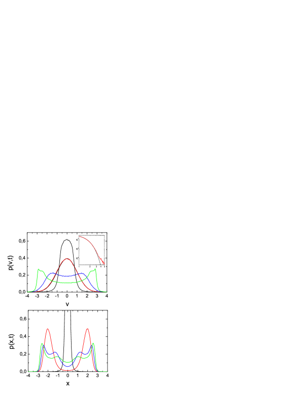
Figure 1: The time-evolution of the probability density distributions obtained from Eq.(9) for $\theta=2$, $\lambda=1$, $T=1$ and $m=1$. Upper part: the velocity distribution for the following times: 2 (green), 10 (blue), 50 (red) and 1 (black) (from left to right on the left-hand side of the figure). The black line which coincides with the case $t=50$ marks the function $\exp(-v^{2}/2)$. Inset: the case $t=50$ in the log-log scale. Lower part: the position distribution for the following times: 5 (green), 10 (blue), 40 (red) and 1 (black).

In order to make the physical meaning of the results more transparent, we rescale the variables to their dimensionless form. The characteristic length is given by the potential size, $L=\sqrt{A/B}$, and the characteristic time $\tau_{0}$ follows from the force balance $mL/\tau_{0}^{2}=\Delta V/L$ lucz where $\Delta V=A^{2}/4B$ is the barrier height; then we have $\tau_{0}=2\sqrt{m/A}$. The dimensionless quantities are the following: $\bar{x}=x/L$, $\bar{v}=\tau_{0}v/L$, $\bar{t}=t/\tau_{0}$, $\bar{\xi}=\xi/AL$, $\bar{w}=mw/AL$, $\bar{\eta}=\eta/AL$, $\bar{\lambda}=\tau_{0}\lambda$, $\bar{\gamma}=\tau_{0}\gamma$, $\bar{c}_{1}=c_{1}/\sqrt{\tau_{0}}$, $\bar{\cal C}={\cal C}/(AL)^{2}$ and $\bar{D}=AL\tau_{0}D$. Eq.(4) takes the form $\bar{\eta}=\bar{K}^{-1}/(1+\theta)|\bar{\xi}|^{1+\theta}\hbox{sgn}(\bar{\xi})$, where $\bar{K}=K/(AL)^{\theta}$. In the following analysis, we use the dimensionless quantities and drop the bar sign. Eq.(II) assumes the form

$$\dot{v}(t) = 4(x-x^{3}-w(t)+c_{1}\sqrt{\lambda}\xi(t))$$

$$\dot{w}(t) = -\lambda w(t)+AL^{2}c_{1}^{2}{\cal C}(0)\lambda v(t)/T$$

$$\dot{x}(t) = v(t)$$

$$\dot{\eta}(t) = -\gamma(1+\theta)\eta(t)+L(t);$$ (12)

moreover, $[m]=$g and $[T]=$g $\hbox{cm}^{2}/\hbox{sec}^{2}$.

III Jumping over a potential barrier

Transport properties of the dynamical systems with the multiplicative noise are different than those for the additive noise. The variance, which always is finite for the Gaussian processes, may rise with time not only linearly but also slower and faster than that, indicating the anomalous diffusion. If the stochastic driving obeys the general Lévy stable statistics, different from the Gaussian, the dynamics with the additive noise implies the accelerated diffusion since the variance is infinite. This rule may not be valid if one introduces the multiplicative factor (2) to the Langevin equation. In the Stratonovich interpretation, the asymptotic form of the probability density distribution is not the same as for the driving noise, in contrast to the Itô interpretation, and depends on $\theta$, $p_{S}(x)\sim|x|^{-1-\alpha-\theta}$. As a consequence, variance may be finite and the system subdiffusive sro09 .

On the other hand, one can ask how long a particle abides in a given area before it finally escapes. This physically important problem has been extensively studied for the Gaussian and Markovian processes and, in particular, a transition rate in the double-well potential was calculated mod . The jumping over a barrier for the case of the Lévy stable noise was analysed in terms of a first passage time distribution in Ref. dyb . MFPT monotonically rises with $\alpha$ for the symmetric noise if both a reflecting and absorbing barrier are assumed. Predictions of the Langevin equation with the multiplicative Lévy stable noise depend, in addition, on the parameter $\theta$ and on a specific interpretation of the stochastic integral sro10 ; sro12b . MFPT initially falls with $\theta$ and then rises which behaviour means – for the Stratonovich interpretation – that the dependence on the effective barrier width is stronger than on the barrier height.

We evaluate the time the particle needs to pass from the right to the left well assuming the initial condition $p(x,0)=\delta(x-x_{m})$. To exclude events of reentering the right well, the point $x=-x_{m}$ is set as an absorbing barrier. However, in the presence of jumps particle may skip the barrier position without hitting it and then the boundary condition must be assumed as nonlocal dyb : $p(x<-x_{m},t)=0$. Moreover, the particle is reflected from the right flank of the potential. The density distribution with the boundary condition, $p(x,t)$, allows us to determine time characteristics of the barrier penetration. The survival probability, i.e. the probability that particle has not yet reached the absorbing barrier, is given by $S(t)=\int_{-x_{m}}^{\infty}p(x,t)dx$. From this quantity the first passage time density distribution directly follows, $f(t)=-dS(t)/dt$, and the averaging over that distribution produces the MFPT:

$$T_{p}=\int_{0}^{\infty}tf(t)dt=\int_{-x_{m}}^{\infty}dx\int_{0}^{\infty}p(x,t)dt.$$ (13)

In the following, we demonstrate how passage statistics depends on the model parameters. Fig.2 presents the survival probability for a fixed temperature and some values of $\lambda$, $\theta$ and $m$. The shape is exponential for all the cases but the rate strongly depends on the parameters, rising with $\lambda$ and diminishing with $m$. Dependence on $\theta$ for small $T$, like the case shown in the figure, is rather complicated. The slope rises with $\theta$ when $\theta$ is large but it becomes very small for small values of this parameter. The exponential shape of $S(t)$ ensures that MFPT is always finite.

Figure 2: The survival probability for $T=1$. The following cases are presented: 1. $\lambda=0.632$, $\theta=2$ and $m=0.1$; 2. $\lambda=0.316$, $\theta=2$ and $m=0.1$; 3. $\lambda=0.316$, $\theta=4$ and $m=0.1$, 4. $\lambda=0.316$, $\theta=2$ and $m=0.5$; 5. $\lambda=0.316$, $\theta=1.2$ and $m=0.1$ (from left to right).

One can expect that MFPT diminishes with the temperature which effect is presented in Fig.3 for some values of $\lambda$ and a fixed $\theta$ ($\gamma$ is different for each value of $\lambda$). MFPT is very large for small values of $T$ and then rapidly falls. Finally it stabilises when the average kinetic energy is sufficiently large to make possible an easy passage above the barrier. The case of the largest memory time, $1/\lambda$, is characterised by a large MFPT and, on the other hand, MFPT becomes small in the white-noise limit. This result may be attributed to a large noise intensity for a large $\lambda$. The function $T_{p}(\theta)$ behaves similarly to $T_{p}(\lambda)$ – the largest $T_{p}$ is observed for small $\theta$ – and that dependence is presented in Fig.4. MFPT decreases with $\theta$ for a given $T$ but only if $\theta$ is relatively small; then it saturates. This behaviour reflects the cosine dependence of the noise intensity on $\theta$: small values of $\theta$ correspond to small noise intensity which approaches zero in the limit $\theta\to 1$. The above observation does not strictly hold in the region of small $T$ since there large values of $\theta$ may lead to relatively large $T_{p}$. This effect is visible also in the next figure.

Figure 3: MFPT as a function of the temperature for $\theta=2$ and $m=0.1$.

Figure 4: MFPT as a function of the temperature for $\lambda=0.316$ and $m=0.1$.

Fig.5 comprises the dependences on all parameters. Since the sensitivity on the potential structure is particularly pronounced at the small temperature, a relatively low value, $T=1$, was chosen. As one may expect, MFPT monotonically increases with the mass and is large for large memory, in agreement with Fig.3. The dependence on $\theta$ for a given $m$ is more complicated. MFPT is largest for a small $\theta$ but then this trend turns to the opposite: the minimum of MFPT corresponds to $\theta=2$ and then its value rises again. Though most of the curves falls monotonically with $\lambda$ and saturates for its large value, the case $\theta=4$ exhibits a clear minimum at $\lambda=1.2$. This non-trivial behaviour may reflect a different dependence of the noise intensity and the damping on both parameters.

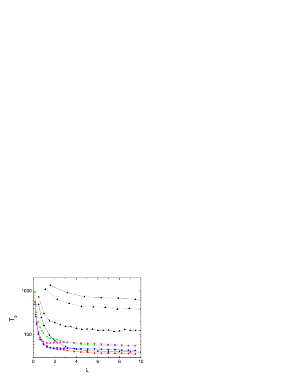
Figure 5: MFPT as a function of $\lambda$ for $T=1$ and different sets of parameters: 1. $\theta=2$ with $m=10,5,1,0.1$ (triangles, from top to bottom), 2. $m=0.1$ with $\theta=4$ (magenta), 1.2 (green), 3 (blue), 1.5 (red) (points, from top to bottom on the right hand side).

IV Stochastic resonance

The possibility that a weak signal may be strengthened by a random perturbation makes the stochastic resonance problem interesting from the point of view of applications. That phenomenon benz consists in matching the noise-induced rate of jumping between the potential wells and the frequency of an external periodic force. It was extensively discussed for the Gaussian noise gamm1 and generalised to the Lévy flights kos ; dybr ; dybr1 . SR is observed also in systems characterised by a multiplicative noise with long jumps sro12b .

Studies of SR are not restricted to the Markovian processes. The non-Markovian features of the dynamics in the context of SR were observed in the framework of a two-state bistable model goy which was a generalisation of the well-known McNamara and Wiesenfeld theory mcn . The residence time distribution appears non-exponential for the non-Markovian case: its shape assumes a stretched-exponential, or even a power-law, form. The SR strength becomes strongly suppressed by the non-Markovian effects goy . This strength used to be measured by a spectral amplification or a signal-to-noise ratio as a function of the temperature. SR was observed in the non-Markovian dynamics for an external, instantaneous noise ful and was studied also for GLE jun1 ; hae ; nei . Properties of SR are strongly influenced by the memory strength (the noise intensity) and time. SR is suppressed by the memory in the overdamped limit but if the coloured noise is induced by inertia, which leads to the Kramers equation, one obtains an enhancement of SR hae . Similar results were obtained in Ref. nei where the kernel comprised an instantaneous friction term and the exponential function. It has been demonstrated that, if the memory time is large, the power amplification rises with both the memory strength and time.

We shall demonstrate that GLE involving jumps also predicts emergence of SR. We consider Eq.(9) where the deterministic force $F(x,t)$ consists of the bistable part (11) and a time-dependent oscillatory force:

$$F(x,t)=-\partial V(x)/\partial x+A_{0}\cos(\omega_{0}t),$$ (14)

where the amplitude $A_{0}$ and the frequency $\omega_{0}$ are constant and dimensionless. The density distribution $p(x,t)$ follows from GLE and can be determined by solving the equations (II). SR emerges if the GLE solution, $x(t)$, is correlated with the periodic stimulation in such a way that the asymptotic amplitude of the output signal, $\bar{x}$, exhibits a maximum when plotted as a function of the noise intensity. This quantity can be expressed in terms of the first Fourier coefficient of the correlation function in the form jun

$$\bar{x}=Re\frac{\omega_{0}}{\pi}\int_{-\infty}^{\infty}dx\int_{0}^{T}xp_{as}(x,t)\exp(i\omega_{0}t)dt,$$ (15)

where $T=2\pi/\omega_{0}$. The distribution $p_{as}(x,t)$ is a long-time limit of $p(x,t)$ and corresponds to the periodic asymptotic solution of GLE. Then, $\bar{x}$ allows us to define the spectral amplification, $\eta=4(\bar{x}/A_{0})^{2}$, which represents a ratio of the integrated power stored in spikes of the power spectrum to the total power carried by the oscillatory force gamm1 .

Figure 6: The spectral amplification for $m=0.1$, $\theta=2$, $\lambda=0.316$ and the following values of $A_{0}$: 1.1, 1.15, 1.225, 1.35, 1.5, 1.65, 1.85, 2, 2.15 and 2.25 (from left to right).

Since response of the system is nonlinear in respect to the system parameters, the spectral amplification depends on the forcing amplitude $A_{0}$; $\eta$ decreases with $A_{0}$ and when it becomes large, the resonance vanishes. On the other hand, for a small $A_{0}$, $\eta$ approaches a value which follows from the linear response theory. However, if the driving frequency $\omega_{0}$ exceeds the Kramers rate, $\eta(A_{0})$ exhibits a maximum gamm1 . Results for our system are presented in Fig.6. In all the calculations we assume $\omega_{0}=5\tau_{0}$ which quantity is relatively large to make the averaging interval small and then to reduce the computation time. Since $\eta$ decreases with $\omega_{0}$ gamm1 , one can expect a moderate amplification. The averaging was started after $t=50/\tau_{0}$ to reach the convergence of $p(x,t)$ to $p_{as}(x,t)$ and to ensure that transients are not present. Results shown in Fig.6 indicate that the amplification decreases with $A_{0}$ for large values of this parameter, the peak shifts toward large $T$ and finally, for $A_{0}>2.2$, the resonant behaviour is no longer observed. The function $\eta(A_{0})$ reaches a maximum at $A_{0}=1.35$, it decreases when $A_{0}$ gets smaller and the resonance vanishes at about $A_{0}=1.1$. From now on, we assume $A_{0}=1.5$.

In the following, we demonstrate how the presence and properties of SR, represented by the function $\eta(T)$, depend on the system parameters. Fig.7 presents $\eta(T)$ for some values of $\lambda$. A peak, indicating a presence of SR, is observed in all the cases and the figure demonstrates that the power amplification is a decreasing function of $\lambda$ in agreement with the Gaussian case in the regime of the large memory time hae ; nei . When $\lambda$ becomes small, the curves acquire an oscillatory structure and the peak finally disintegrates. This phenomenon is observed in the figure for a very large memory time, $\lambda=0.158$. On the other hand, the oscillations vanish in the white-noise limit (large $\lambda$). The position of the peak shifts to the right with increasing $\lambda$.

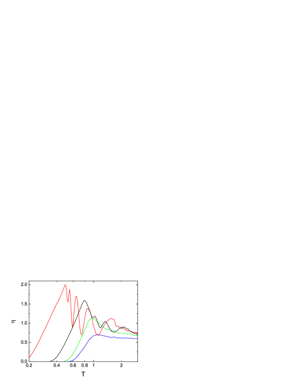
Figure 7: The spectral amplification for $m=0.1$, $\theta=2$ and the following values of $\lambda$: 0.158, 0.316, 0.474 and 0.632 (from left to right).

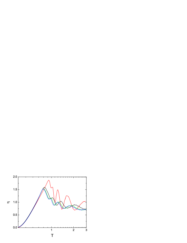
Figure 8: The spectral amplification for $m=0.1$, $\lambda=0.316$ and the following values of $\theta$: 1.2, 2, 3 and 4 (from top to bottom).

The parameter $\theta$ is responsible for the slope of the noise distribution, namely a large $\theta$ makes it steeper and reduces the variance of $\xi(t)$. Moreover, it influences the memory time $\lambda$. The dependence of the power amplification on $\theta$ for a fixed $\lambda$, which means that $\gamma$ depends on $\theta$, is presented in Fig.8. The results are sensitive on $\theta$ when it approaches the value $\theta=1$, corresponding to the vanishing noise intensity; then $\eta$ is largest and oscillations are strong. For larger $\theta$, dependence of $\eta(T)$ on $\theta$ is very weak.

Figure 9: The spectral amplification for $\lambda=0.316$, $\theta=2$ and the following values of $m$: 0.09, 0.1, 0.12, 0.15 and 0.2 (from right to left).

Finally, we consider the dependence of the spectral amplification of the inertia and those results are presented in Fig.9. Large values of $m$ correspond to a small intensity of SR and smooth peaks with a sharp cut-off at the left-hand side. For simple systems, the slopes of the peaks on the right-hand side are determined by the potential: they fall to zero if it is asymptotically strong and may rise for soft potentials hei . In the present case, the slopes stabilise at a constant value. For a smaller mass, the peaks are wider and their height rises when $m$ decreases but finally it saturates. The SR position shifts to the left with the increasing $m$.

V Summary and conclusions

The characteristic features of the generalised Ornstein-Uhlenbeck process $\xi(t)$, including the multiplicative Cauchy noise, are long tails of the distribution, a finite variance and a finite correlation time. Those properties are typical for the complex systems and the multiplicative noise reflects a dependence of the random force on the process value, which may result, in particular, from a nonhomogeneity of the space. The process $\xi(t)$ is defined by two parameters: the damping $\gamma$ and the multiplicative noise parameter $\theta$. Both of them determine the relaxation rate $\lambda$, as well as the variance which decreases with $\theta$ and $\gamma$. If $\xi(t)$ represents an internal effective noise in a dynamical system, its finite correlation time requires a retarded friction to satisfy the fluctuation-dissipation theorem. We discussed the dynamics governed by GLE in which, beside $\xi(t)$, the double-well potential was included. The solutions of GLE produce the velocity density distributions which converge to a distribution resembling the Gaussian. However, it possesses the power-law tails, similarly to the case without any potential. In the latter case, when the system is linear, this apparent violation of the central limit theorem is an effect of large higher moments.

The transport properties, quantified in terms of MFPT, were discussed for all model parameters. MFPT declines with $T$ and $\lambda$ whereas it rises with $m$. The dependence on $\theta$ is not monotonic and complicated for large $\theta$ being different for the low and high temperature. The survival probability always reveals the exponential form.

When the deterministic potential is supplemented by a time-dependent oscillatory force, the stochastic resonance emerges. It was studied by evaluating the spectral amplification $\eta$ as a function of the temperature. Both the intensity of SR and its position strongly depend on the memory parameter $\lambda$: the smaller $\lambda$ the stronger amplification and the peak positioned at a lower temperature. The variability of the above quantities with $\theta$, in turn, is less pronounced and actually restricted to a region of small values of this parameter where the amplification is large. A striking feature of the curves corresponding to small values of either $\lambda$ or $\theta$ is their oscillatory structure which is observed neither for GLE in the Gaussian case nei nor for the Langevin equation with the multiplicative noise with jumps sro12b . This structure emerges when the noise intensity is small and memory long, i.e. when trajectories are trapped in the well for a long time (large MFPT). The dependence of the SR properties on the inertia is simple and the intensity of SR rises when the mass becomes smaller but finally $\eta$ stabilises at a relatively large value.

References

- (1) T. Srokowski, Phys. Rev. E 80, 051113 (2009)
- (2) T. Srokowski, Phys. Rev. E 87, 032104 (2013)
- (3) H. Mori, Prog. Theor. Phys. 33, 423 (1965); ibid 34, 399 (1965)
- (4) R. Kubo, Rep. Prog. Phys. 29, 255 (1966)
- (5) W. Feller, An introduction to probability theory and its applications (John Wiley and Sons, New York, 1966), Vol.II.
- (6) W. T. Coffey, Yu. P. Kalmykov, J. T. Waldron, The Langevin Equation (World Scientific, Singapore, 2004)
- (7) M. Kostur, J. Łuczka, P. Hänggi, Phys. Rev. E 80, 051121 (2009)
- (8) L. Machura, J. Łuczka, Phys. Rev. E 82, 031133 (2010)
- (9) R. L. S. Farias, R. O. Ramos, L. A. da Silva, Phys. Rev. E 80, 031143 (2009)
- (10) P. Siegle, I. Goychuk, P. Hänggi, Europh. Lett. 93, 20002 (2011)
- (11) P. Hänggi, P. Talkner, M. Borkovec, Rev. Mod. Phys. 62, 251 (1990)
- (12) B. Dybiec, E. Gudowska-Nowak, P. Hänggi, Phys. Rev. E 75, 021109 (2007)
- (13) T. Srokowski, Phys. Rev. E 81, 051110 (2010)
- (14) T. Srokowski, Eur. Phys. J. B 85, 65 (2012)
- (15) R. Benzi, A. Sutera, A. Vulpiani, J. Phys. A 14, L453 (1981)
- (16) L. Gammaitoni, P. Hänggi, P. Jung, F. Marchesoni, Rev. Mod. Phys. 70, 223 (1998)
- (17) B. Kosko, S. Mitaim, Phys. Rev. E 64, 051110 (2001)
- (18) B. Dybiec, E. Gudowska-Nowak, J. Stat. Mech., P05004 (2009)
- (19) B. Dybiec, Phys. Rev. E 80, 041111 (2009)
- (20) I. Goychuk, P. Hänggi, Phys. Rev. E 69, 021104 (2004)
- (21) B. McNamara, K. Wiesenfeld, Phys. Rev. A 39, 4854 (1989)
- (22) A. Fuliński, Phys. Rev. E 52, 4253 (1995)
- (23) P. Jung, P. Hänggi, Phys. Rev. A 41, 2977 (1990)
- (24) P. Hänggi, P. Jung, C. Zerhe, F. Moss, J. Stat. Phys. 70, 25 (1993)
- (25) A. Neiman, W. Sung, Phys. Lett. A 223, 341 (1996)
- (26) P. Jung, P. Hänggi, Phys. Rev. A 44, 8032 (1991)
- (27) E. Heinsalu, M. Patriarca, F. Marchesoni, Eur. Phys. J. B 69, 19 (2009)