Soft-gluon Resummation for High-$p_{T}$ Inclusive-Hadron Production at COMPASS

Abstract

We study the cross section for the photoproduction reaction $\gamma N\rightarrow hX$ in fixed-target scattering at COMPASS, where the hadron $h$ is produced at large transverse momentum. We investigate the role played by higher-order QCD corrections to the cross section. In particular we address large logarithmic “threshold” corrections to the rapidity dependent partonic cross sections, which we resum to all orders at next-to-leading accuracy. In our comparison to the experimental data we find that the threshold contributions are large and improve the agreement between data and theoretical predictions significantly.

I Introduction

Photoproduction processes in fixed-target lepton-nucleon scattering are important probes of nucleon structure. Cross sections for high-transverse-momentum ($p_{T}$) final states typically receive sizable or even dominant contributions from the photon-gluon fusion subprocess $\gamma g\to q\bar{q}$, offering access to the nucleon’s gluon distribution that is otherwise hard to obtain in lepton scattering. Notably, the fixed target lepton scattering experiment COMPASS at CERN uses the process $\gamma N\rightarrow hX$ (where $h$ denotes a high-$p_{T}$ final-state hadron) in polarized scattering in order to determine the nucleon’s gluon helicity distribution $\Delta g$ Silva (2011). Earlier measurements were made by the SLAC E155 experiment Anthony et al. (1999). Such measurements may provide information complementary to that obtained in polarized $pp$-scattering at RHIC Aschenauer et al. (2013).

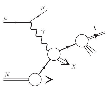
Figure 1: Photoproduction in lepton-nucleon scattering. The virtual photon is required experimentally to have low virtuality.

At COMPASS, photoproduction $\gamma N\rightarrow hX$ is accessed in the lepton-nucleon scattering process $\mu N\to\mu^{\prime}hX$ by selecting events with low virtuality of the exchanged photon (see Fig. 1), typically $Q^{2}=-q^{2}\leq 0.1\,{\rm GeV}^{2}$. Such a selection is favored over deep-inelastic scattering at large $Q^{2}$ in terms of statistics since most of the events in lepton scattering are clustered at low $Q^{2}$. As long as the produced hadron’s transverse momentum is large, the reaction can still be considered a hard-scattering reaction. From a theoretical point of view, however, the framework for the process $\gamma N\rightarrow hX$ in fixed-target scattering is relatively complex. While the radiation of the quasi-real photon from the incident lepton can be straightforwardly treated by the Weizsäcker-Williams equivalent photon method, the interaction of the photon with the nucleon requires additional input as compared to usual deep-inelastic scattering. First, it is well known that a quasi-real photon does not always interact in an elementary “direct” way, but may also resolve into its own hadronic structure, described by parton distributions of the photon. Although some of these resolved contributions also involve the nucleon’s gluon distribution, they will overall tend to dilute the sensitivity of photoproduction to the gluon density somewhat. For unpolarized photons, measurements at HERA and LEP have provided a fair amount of information on the photon’s parton distributions (for review, see Klasen (2002)), so that the resolved components in the cross section may be computed relatively reliably. In the polarized case, very little is known about the photon’s parton content. Estimates based on next-to-leading order calculations have shown here Jäger et al. (2005); Jäger et al. (2003a) (see also Afanasev et al. (1998)) that the process remains a good probe of $\Delta g$ even in the presence of resolved contributions.

The other reason why theoretical calculations are quite involved is due to the fixed-target kinematics employed in experiment. Typically transverse momenta are such that the variable $x_{T}=2p_{T}/\sqrt{s}$ (with $\sqrt{s}$ the center-of-mass energy) is relatively large, say, $x_{T}\gtrsim 0.1$. It turns out that the partonic hard-scattering cross sections relevant for $\gamma N\rightarrow hX$ are then largely probed in the “threshold”-regime, where the initial photon and parton have just enough energy to produce the high-transverse momentum parton that subsequently fragments into the hadron, and its recoiling counterpart. Relatively little phase space is then available for additional radiation of partons. In particular, gluon radiation is inhibited and mostly constrained to the emission of soft and/or collinear gluons. The cancellation of infrared singularities between real and virtual diagrams then leaves behind large double- and single-logarithmic corrections to the partonic cross sections. These logarithms appear for the first time in the next-to-leading order (NLO) expressions for the partonic cross sections, where (for the rapidity-integrated cross section) they arise as terms of the form $\alpha_{s}\ln^{2}(1-x_{T}^{2})$, with $\alpha_{s}$ the strong coupling constant. At yet higher ($k$th) order of perturbation theory, the double-logarithms are of the form $\alpha_{s}^{k}\ln^{2k}(1-x_{T}^{2})$. When the threshold regime dominates, it is essential to take into account the large logarithms to all orders in the strong coupling, a technique known as “threshold resummation”. For single-hadron production in $pp\to hX$ in the fixed-target regime, the resummation has been carried out in de Florian and Vogelsang (2005), and substantial effects were observed that lead to an enhancement of the cross section. The same was found for the related process $pp\to h_{1}h_{2}X$ Almeida et al. (2009). It is therefore to be expected that threshold resummation effects are also relevant for the process $\gamma N\rightarrow hX$.

In the present paper we will address this issue and investigate the resummation effects on the spin-averaged cross section for $\gamma N\rightarrow hX$ in the COMPASS kinematic regime. Resummation affects the direct and the resolved contributions to the cross section differently, which makes photoproduction a particularly interesting process from the point of view of resummation. Our results are directly relevant for comparison to recent COMPASS data Adolph et al. (2012); Höppner (2012). We note that we also extend the previous work de Florian and Vogelsang (2005) by including rapidity dependence in resummation, following the techniques developed in Almeida et al. (2009). In our phenomenological studies we find that the threshold logarithms play an important role for COMPASS kinematics, yielding essential higher-order corrections. Thus, resummation turns out to be a vital ingredient for comparisons between theory and experimental data.

The paper is organized as follows. In Sec. II we recall the basic framework for photoproduction of a hadron. In Section III we present details of threshold resummation and describe the technique that enables us to get a resummed expression for fixed rapidity of the observed hadron. Section IV is devoted to a phenomenological analysis, focusing on the kinematics of the COMPASS experiment. We briefly conclude in Sec. V.

II Technical framework

We consider the unpolarized cross section for the semi-inclusive process

$$\ell N\rightarrow\ell^{\prime}h^{\pm}X,$$ (1)

where a lepton beam scatters off a nucleon target $N$ producing a hadron $h$ with transverse momentum $p_{T}$ and pseudorapidity $\eta$ in the final state. The basic concept that links the experimentally measurable quantities to theoretical predictions made from perturbative calculations is the factorization theorem. It states that large momentum-transfer reactions may be split into long-distance pieces, the universal parton distribution functions, and short-distance contributions reflecting the hard interactions of the partons. Thus we may write the unpolarized rapidity dependent differential cross section for the process in Eq. (1) as the following convolution Collins et al. (1985); Sterman (1987):

$$\frac{p_{T}^{3}d\sigma}{dp_{T}d\eta}=\sum_{a,b,c}\int_{x_{\ell}^{{\mathrm{min}}}}^{1}dx_{\ell}\int_{x_{n}^{{\mathrm{min}}}}^{1}dx_{n}\int_{x}^{1}dz\frac{\hat{x}_{T}^{4}z^{2}}{8v}$$

$$\times f_{a/\ell}(x_{\ell},\mu_{fi})f_{b/N}(x_{n},\mu_{fi})D_{h/c}(z,\mu_{ff})\frac{\hat{s}d\hat{\sigma}_{ab\rightarrow cX}}{dvdw}\,.$$ (2)

The sum in Eq. (2) extends over all possible partonic channels with $\hat{\sigma}_{ab\rightarrow cX}$ denoting the associated partonic hard scattering cross section. In addition to the renormalization scale $\mu_{r}$, the factorization of the hadronic cross section requires the introduction of two further scales: the factorization scales $\mu_{fi},\mu_{ff}$ for the initial and final states, respectively. All scales are arbitrary but should be of the order of the hard scale. One usually chooses them to be equal, typically $\mu_{r}=\mu_{fi}=\mu_{ff}=p_{T}$. The parton distributions of the lepton and the nucleon, $f_{a/\ell}(x_{\ell},\mu_{fi}),f_{b/N}(x_{n},\mu_{fi})$, are evolved to the factorization scale and depend on the respective momentum fractions $x_{\ell,n}$ carried by partons $a$ and $b$. $D_{h/c}(z,\mu_{ff})$ denotes the parton-to-hadron fragmentation function. The lower bounds in the integrations over the various momentum fractions in Eq. (2) read:

$$x_{\ell}^{{\mathrm{min}}}=\frac{x_{T}e^{\eta}}{2-{x_{T}}e^{-\eta}},~{}x_{n}^{{\mathrm{min}}}=\frac{x_{T}e^{-\eta}}{2-\frac{x_{T}}{x_{\ell}}e^{\eta}},~{}x=\frac{x_{T}\cosh\hat{\eta}}{\sqrt{x_{n}x_{\ell}}}.$$ (3)

Here $\hat{\eta}$ and $\hat{x}_{T}$ are the partonic counterparts to the pseudorapidity $\eta$ and the hadronic scaling variable $x_{T}=2p_{T}/\sqrt{s}$,

$$\hat{\eta}=\eta+\frac{1}{2}\ln{\frac{x_{n}}{x_{\ell}}},~{}\hat{x}_{T}=\frac{x_{T}}{z\sqrt{x_{\ell}x_{n}}}\,.$$ (4)

It is common convention to introduce two variables $v$ and $w$,

$$v=1-\frac{\hat{x}_{T}}{2}e^{-\hat{\eta}},~{}w=\frac{1}{v}\frac{\hat{x}_{T}}{2}e^{\hat{\eta}}\,,$$ (5)

and to rewrite the partonic cross section in terms of this new set of variables. Furthermore we introduce the Mandelstam variables

$$\hat{s} =x_{n}x_{\ell}s,~{}~{}\hat{t}=(p_{a}-p_{c})^{2}=-\hat{s}\hat{x}_{T}e^{-\hat{\eta}}/2,$$

$$\hat{u} =(p_{b}-p_{c})^{2}=-\hat{s}\hat{x}_{T}e^{\hat{\eta}}/2.$$ (6)

The invariant mass of the unobserved partonic final state is

$$s_{4}=\hat{s}+\hat{t}+\hat{u}=\hat{s}v(1-w)=\hat{s}(1-\hat{x}_{T}\cosh\hat{\eta}).$$ (7)

The partonic hard-scattering functions $\hat{\sigma}_{ab\rightarrow cX}$ can be evaluated in QCD perturbation theory. They may each be written as an expansion in the strong coupling constant $\alpha_{s}(\mu_{r})$ of the form

$$\hat{\sigma}_{ab\rightarrow cX}(v,w)=\hat{\sigma}_{ab\rightarrow cX}^{(0)}(v,w)+{\alpha_{s}(\mu_{r})}\hat{\sigma}_{ab\rightarrow cX}^{(1)}(v,w)+\mathcal{O}(\alpha_{s}^{2}).$$ (8)

Whenever a photon takes part in a hard scattering process as initial particle, one generally distinguishes two contributions, the so-called “direct” and “resolved” photon contributions,

$$d\sigma=d\sigma_{\rm dir}+d\sigma_{\rm res}.$$ (9)

Applying the Weizsäcker-Williams equivalent photon method to the lepton-to-parton distribution functions, $f_{a/\ell}$ in Eq. (2) may be written as a convolution of a lepton-to-photon splitting function $P_{\gamma\ell}$ and a parton distribution function $f_{a/\gamma}$ of a photon:

$$f_{a/\ell}(x_{\ell},\mu_{f})=\int_{x_{\ell}}^{1}\frac{dy}{y}P_{\gamma\ell}(y)f_{a/\gamma}(x_{\gamma}=\frac{x_{\ell}}{y},\mu_{f}).$$ (10)

In the unpolarized case the splitting function is given by Frixione et al. (1993); de Florian and Frixione (1999)

$$\begin{aligned} P_{\gamma\ell}(y)=\frac{\alpha}{2\pi}\left[\frac{1+(1-y^{2})}{y}\ln\frac{Q^{2}_{\rm max}(1-y)}{m_{\ell}^{2}y^{2}}\right.\\ +\left.2m_{\ell}^{2}y\left(\frac{1}{Q^{2}_{\rm max}}-\frac{1-y}{m_{\ell}^{2}y^{2}}\right)\right],\end{aligned}$$ (11)

and describes the collinear emission of a quasi-real photon with momentum fraction $y$ off a lepton $\ell$ of mass $m_{\ell}$. The virtuality of the radiated photon is restricted to be less than $Q_{\rm max}$, which is in turn constrained by the experimental setup.

In the direct case, the photon participates as a whole and parton $a$ in Eq. (2) is an elementary photon. Consequently, we here have simply

$$f_{\gamma/\gamma}(x_{\gamma},\mu_{f})=\delta(1-x_{\gamma}).$$ (12)

There are two basic partonic subprocesses in lowest order (LO), in which a photon and a parton from the initial nucleon give rise to the production of a hadron: photon-gluon-fusion $\gamma g\to q\bar{q}$ and Compton scattering $\gamma q\to qg$. For each process, either of the final-state partons may hadronize into the observed hadron. As the processes are partly electromagnetic and partly due to strong interaction their cross sections are proportional to $\alpha\alpha_{s}(\mu_{r})$, where $\alpha$ represents the electromagnetic fine structure constant.

In addition to that the photon exhibits also a hadronic structure in the framework of QCD. This is described by the resolved process. Unlike hadronic parton distributions, photonic densities may be decomposed into a purely perturbatively calculable “pointlike” contribution and a nonperturbative “hadron-like” part. While the pointlike contribution dominates at large momentum fractions $x_{\gamma}$, the latter dominates in the low-to-mid $x_{\gamma}$ region and may be estimated via the vector-meson-dominance model Schuler and Sjostrand (1996); Glück et al. (1999). At lowest order there are the following resolved subprocesses:

$$qq^{\prime}\rightarrow qq^{\prime},~{}~{}q\bar{q}^{\prime}\rightarrow q\bar{q}^{\prime},~{}~{}q\bar{q}\rightarrow q^{\prime}\bar{q}^{\prime},~{}~{}qq\rightarrow qq,~{}~{}q\bar{q}\rightarrow q\bar{q},$$

$$q\bar{q}\rightarrow gg,~{}~{}gq\rightarrow qg,~{}~{}qg\rightarrow gq,~{}~{}gg\rightarrow gg,~{}~{}gg\rightarrow q\bar{q}.$$ (13)

Each of these is a pure QCD-process and therefore has a cross section quadratic in $\alpha_{s}(\mu_{r})$. However, as the photon parton distributions are formally of order $\alpha/\alpha_{s}(\mu_{f})$, the perturbative expansion of the direct and resolved contributions starts at the same order.

At LO where one has $2\rightarrow 2$ kinematics, $w\equiv 1$, and therefore,

$$\frac{\hat{s}d\hat{\sigma}^{(0)}_{ab\rightarrow cX}(v,w)}{dvdw}=\frac{\hat{s}d\hat{\sigma}^{(0)}_{ab\rightarrow cd}(v)}{dv}\delta(1-w).$$ (14)

The numerous partonic NLO cross sections $\hat{\sigma}^{(1)}_{ab\rightarrow cX}(v,w)$ have been computed in Aversa et al. (1989); Jäger et al. (2003b). They can be cast into the form

$$\frac{\hat{s}d\hat{\sigma}^{(1)}_{ab\rightarrow cX}(v,w)}{dvdw}= A(v)\delta(1-w)+B(v)\left(\frac{\ln(1-w)}{1-w}\right)_{+}$$

$$+C(v)\left(\frac{1}{1-w}\right)_{+}+F(v,w).$$ (15)

Here the “+”-distributions are defined as follows:

$$\int_{0}^{1}f(w)[g(w)]_{+}dw=\int_{0}^{1}[f(w)-f(1)]g(w)dw.$$ (16)

The function $F(v,w)$ collects all remaining terms that do not contain any distributions. The terms in Eq. (15) associated with “+”-distributions yield large logarithmic first order corrections close to the threshold. These terms can be traced back to soft gluon emission and will also show up in all higher order corrections. For each new order of perturbations theory one is faced with two more powers of leading logarithmic contributions. To be specific, in the $k$th order in perturbation theory $d\hat{\sigma}^{(k)}_{ab\rightarrow cX}(v,w)/dvdw$ contains logarithms of the form $\alpha_{s}^{k}[\ln^{2k-1}(1-w)/(1-w)]_{+}$, plus subleading terms with fewer logarithms. Depending on kinematics, these logarithmic terms have to be resummed order-by-order.

III Resummed cross section

In this section we will provide the resummed differential cross section as a function of transverse momentum $p_{T}$ and pseudorapidity $\eta$ of the produced hadron.

III.1 Mellin moments and threshold region

Threshold resummation of soft gluon emissions is performed in Mellin-$N$ moment space. Taking Mellin moments transforms a convolution of a parton distribution function and the partonic cross section into a product of moments of the corresponding quantities. The threshold region $w\rightarrow 1$ corresponds to large Mellin moments. Under this transformation, the large soft-gluon corrections showing up as “+”-distributions are translated into powers of logarithms $\ln N$. This logarithmic behavior colludes with the $N$-dependence of the parton distribution functions and the fragmentation function, which in moment space typically fall off as $1/N^{4}$ or faster at large $N$.

The single-inclusive cross section we are interested in here depends on two kinematic variables, $p_{T}$ and $\eta$. If the cross section is integrated over all rapidities, it becomes a function of $x_{T}^{2}$, and a single Mellin moment in $x_{T}^{2}$ suffices to factorize it in terms of moments of parton distributions, fragmentation functions, and partonic cross sections de Florian and Vogelsang (2005). After resummation the full Mellin expression is inverted, directly giving the desired hadronic cross section. If, on the other hand, one is interested in the rapidity dependence of the resummed cross section, the integrations of the various functions in Eq. (2) are no longer convolutions in a strict sense, and a different technique needs to be used. A convenient possibility Almeida et al. (2009) is to use Mellin moments for only a part of the terms in Eq. (2). That is, one takes Mellin moments only of the product of fragmentation functions and the resummed partonic cross sections, performs a Mellin inverse, and convolutes the result with the parton distributions in $x$-space. Inclusion of the fragmentation functions in the Mellin moment expression guarantees that the integrand for the inverse Mellin transform falls off fast enough for the integral to show good numerical convergence. On the other hand, performing the convolution with the parton distributions in $x$-space provides full control over rapidity, since the partonic and hadronic rapidities are related by a boost along the collision axis that involves only the momentum fractions of the initial-state partons.

To be specific, starting from Eq. (2), we consider only the last integral and take moments in $x^{2}$ (where $x$ is the lower bound of the $z$-integral). The integral then factorizes into a product of moments:

$$\int_{0}^{1}dx^{2}\,(x^{2})^{N-1}\int_{x}^{1}dz\frac{\hat{x}_{T}^{4}z^{2}}{8v}D_{h/c}(z,\mu_{ff})\frac{\hat{s}d\hat{\sigma}_{ab\rightarrow cX}}{dvdw}$$

$$\equiv\,D_{h/c}^{2N+3}(\mu_{ff})\tilde{w}^{2N}(\hat{\eta}),$$ (17)

where the Mellin moments $D_{h/c}^{N}(\mu_{ff})$ of the fragmentation function are defined as usual by

$$D_{h/c}^{N}(\mu_{ff})=\int_{0}^{1}dzz^{N-1}D_{h/c}(z,\mu_{ff}),$$ (18)

and where the hard scattering function $\tilde{w}^{N}(\hat{\eta})$ is given in Mellin-$N$ moment space by

$$\tilde{w}^{N}(\hat{\eta})=2\int_{0}^{1}d\frac{s_{4}}{\hat{s}}\left(1-\frac{s_{4}}{\hat{s}}\right)^{N-1}\frac{\hat{x}_{T}^{4}z^{2}}{8v}\frac{\hat{s}d\hat{\sigma}_{ab\rightarrow cX}}{dvdw}.$$ (19)

We next take the Mellin inverse of the expression in Eq. (17) which is then convoluted with the parton distributions:

$$\frac{p_{T}^{3}d\sigma}{dp_{T}d\eta}= \sum_{a,b,c}\int_{0}^{1}dx_{\ell}\int_{0}^{1}dx_{n}f_{a/\ell}(x_{\ell},\mu_{fi})f_{b/N}(x_{n},\mu_{fi})$$

$$\times\int_{\cal{C}}\frac{dN}{2\pi i}(x^{2})^{-N}D_{h/c}^{2N+3}(\mu_{ff})\tilde{w}^{2N}(\hat{\eta}).$$ (20)

This is mathematically equivalent to using Eq. (2) in the first place. However, once one uses a resummed hard-scattering function, it is much better from a computational point of view to use the procedure in (20) since the moments of the fragmentation functions tame the large-$N$ behavior of the $\tilde{w}^{2N}$ so that the Mellin integral converges rapidly. In contrast, to carry out a convolution over $z$ as in Eq. (2) would become very difficult for a resummed hard-scattering function, since the latter contains “+”-distributions with any power of a logarithm.

III.2 Rapidity-dependent resummation to next-to-leading logarithm

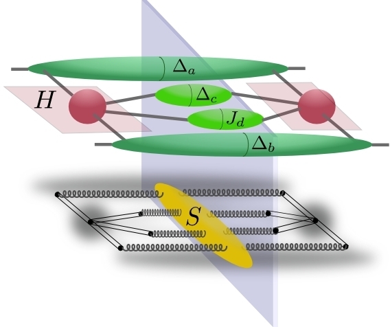
Figure 2: Schematic illustration of the factorization of the cross section close to threshold. The plane symbolizes the cut, which separates the amplitude and its complex conjugte. For each of the initial- and final-state partons there is a function ($\Delta_{a,b,c},J_{d}$) describing soft-gluon emissions off these partons. The hard-scattering part $H$ is depicted as amplitude and its complex conjugate. It can be completely separated from the soft function $S$, shown in the lower part of the figure. The double lines represent eikonal lines.

It turns out that multigluon QCD amplitudes factorize to logarithmic accuracy. Furthermore, in Mellin space, also the phase space including the constraint of energy conservation factorizes. The resummed cross section in moment space factorizes into functions for each single participating parton, a function describing the hard scattering, and a soft function. This factorization is illustrated in Fig. 2. The resummed cross section is given by Kidonakis and Sterman (1997); Kidonakis et al. (1998a, b); Bonciani et al. (2003):

$$\tilde{w}^{{\mathrm{resum}},N}_{ab\rightarrow cd}(\hat{\eta})= \Delta_{a}^{N_{a}}(\hat{s},\mu_{fi})\Delta_{b}^{N_{b}}(\hat{s},\mu_{fi})\Delta_{c}^{N}(\hat{s},\mu_{ff})$$

$$\times J_{d}^{N}(\hat{s}){\mathrm{Tr}}\left\{H\mathcal{S}_{N}^{\dagger}S\mathcal{S}_{N}\right\}_{ab\rightarrow cd},$$ (21)

where $N_{a}=(-\hat{u}/\hat{s})N$ and $N_{b}=(-\hat{t}/\hat{s})N$. The resummed exponents for the initial-state partons ${a,b=q,\bar{q},g}$ in Eq. (21) read, in the $\overline{\text{MS}}$ scheme:

$$\ln\Delta_{i}^{N}(M_{i}^{2},\mu_{fi})= -\int_{0}^{1}dz\frac{z^{N-1}-1}{1-z}$$

$$\times\left\{\int_{(1-z)^{2}}^{1}\frac{dt}{t}A_{i}\left[\alpha_{s}\left(tM_{i}^{2}\right)\right]\right.$$

$$+\left.\bar{B}_{i}\left(\nu_{i},\frac{M_{i}^{2}}{\hat{s}},\alpha_{s}\left((1-z)^{2}M_{i}^{2}\right)\right)\right\}$$

$$-2\int_{\mu_{r}}^{M_{i}}\frac{d\mu^{\prime}}{\mu^{\prime}}\gamma_{i}\left(\alpha_{s}(\mu^{\prime 2})\right)$$

$$+2\int_{\mu_{fi}}^{M_{i}}\frac{d\mu^{\prime}}{\mu^{\prime}}\gamma_{ii}\left(N,\alpha_{s}(\mu^{\prime 2})\right).$$ (22)

Here $M_{i}$ is a scale of order $\sqrt{\hat{s}}$. It was shown that the exponent is in fact independent of $M_{i}$ at next-to-leading logarithmic (NLL) accuracy Sterman and Vogelsang (2001). Furthermore, we have

$$A_{i}(\alpha_{s})=C_{i}[{\alpha_{s}}/{\pi}+({K}/2)\left({\alpha_{s}}/{\pi}\right)^{2}],$$

$$\bar{B}_{i}(\nu_{i},M_{i}^{2}/\hat{s},\alpha_{s})=C_{i}(\alpha_{s}/\pi)[1-\ln(2\nu_{i})+\ln(M_{i}^{2}/\hat{s})],$$ (23)

where $K=C_{A}[{67}/{18}-{\pi^{2}}/{6}]-5/9N_{f}$, $C_{i}=C_{q}=C_{F}=4/3$ for an incoming quark, and $C_{i}=C_{g}=C_{A}=3$ for a gluon. $N_{f}$ denotes the number of flavors. The $\nu_{i}$ are defined as

$$\nu_{i}\equiv\frac{(\beta_{i}\cdot n)^{2}}{|n^{2}|},$$ (24)

with the parton velocity $\beta_{i}^{\mu}=p^{\mu}_{i}\sqrt{2/\hat{s}}$ and an axial gauge vector $n$. The $\nu_{i}$ were introduced to make the factorization of the cross section manifest Laenen et al. (1998). The gauge-dependence they express will cancel in the final resummed cross section. The last two terms in Eq. (22) match the exponent to the chosen renormalization and factorization scale, respectively. The $\gamma_{i}$ are the anomalous dimensions of the quark and gluon fields, and the $\gamma_{ii}$ correspond to the logarithmic and constant terms of the moments of the diagonal Altarelli-Parisi splitting functions. To one loop order, one has

$$\gamma_{q}(\alpha_{s})=\frac{3}{4}C_{F}\frac{\alpha_{s}}{\pi},~{}~{}\gamma_{qq}(N,\alpha_{s})=-\left(\ln N-\frac{3}{4}\right)C_{F}\frac{\alpha_{s}}{\pi},$$

$$\gamma_{g}(\alpha_{s})=b_{0}\alpha_{s},~{}~{}~{}~{}~{}~{}\gamma_{gg}(N,\alpha_{s})=-\left(C_{A}\ln N-\pi b_{0}\right)\frac{\alpha_{s}}{\pi},$$ (25)

where $b_{0}=4\pi\beta_{0}=(11C_{A}-4T_{R}N_{f})/(12\pi)$, with $T_{R}=1/2$ and the one-loop coefficient of the $\beta$-function, $\beta_{0}$. We note that the large-$N$ behavior of the diagonal splitting functions and anomalous dimensions links the various terms in the exponent in Eq. (22) to each other,

$$\gamma_{ii}(N,\alpha_{s})=-\ln\bar{N}A_{i}(\alpha_{s})+\gamma_{i}(\alpha_{s}),$$ (26)

where $\bar{N}=Ne^{\gamma_{E}}$ with the Euler constant $\gamma_{E}$.

For the direct processes, parton $a$ is a photon and we have simply $\Delta_{\gamma}^{N_{a}}(\hat{s},\mu_{fi})=1$. For the fragmenting parton $c$ one has the same exponent as for the incoming partons $\Delta_{i}^{N}(M_{i}^{2})$ in Eq. (22), but with the final state factorization scale $\mu_{ff}$ in place of the initial-state one.

The exponential function $J_{d}^{N}$ in Eq. (21) contains collinear emission, both soft and hard, by the unobserved final-state jet that recoils against the observed parton. It is independent of factorization scale and is given by

$$\ln J_{d}^{N}(\hat{s})= \int_{0}^{1}dz\frac{z^{N-1}-1}{1-z}\left\{\int_{(1-z)^{2}}^{(1-z)}\frac{dt}{t}A_{d}[\alpha_{s}(t\hat{s})]\right.$$

$$-\gamma_{d}[\alpha_{s}((1-z)\hat{s})]-\bar{B}_{d}[\nu_{d},1,\alpha_{s}((1-z)^{2}\hat{s})]{\bigg{\}}}$$

$$+2\int_{\mu_{r}}^{\sqrt{\hat{s}}}\frac{d\mu^{\prime}}{\mu^{\prime}}\gamma_{d}(\alpha_{s}(\mu^{\prime 2})),$$ (27)

where $A_{d}$, $\gamma_{d}$ and $\bar{B}_{d}$ are defined as in Eq. (23).

Finally, coherent soft gluon radiation among the jets is treated by the last term in Eq. (21). The functions $H_{ab\rightarrow cd}$, $\mathcal{S}_{N,{ab\rightarrow cd}}$ and $S_{ab\rightarrow cd}$ are matrices in a space of color exchange operators Kidonakis and Sterman (1997); Kidonakis et al. (1998a, b), and the trace is taken in this color space. The $H_{ab\rightarrow cd}$ are the hard-scattering functions. They are perturbative series in $\alpha_{s}$,

$$H_{ab\rightarrow cd}(\hat{\eta},\alpha_{s})=H_{ab\rightarrow cd}^{(0)}(\hat{\eta})+\frac{\alpha_{s}}{\pi}H_{ab\rightarrow cd}^{(1)}(\hat{\eta})+\mathcal{O}(\alpha_{s}^{2}).$$ (28)

The LO contributions to the hard-scattering functions in the resolved-photon case are known with their full color dependence Kidonakis and Sterman (1997); Kidonakis et al. (1998a, b); Kidonakis and Owens (2001), and the NLO terms have been obtained in Kelley and Schwartz (2011); Catani et al. (2013). The $S_{ab\rightarrow cd}$ are soft functions and may be expanded as

$$S_{ab\rightarrow cd}(\hat{\eta},\alpha_{s})=S_{ab\rightarrow cd}^{(0)}+\frac{\alpha_{s}}{\pi}S_{ab\rightarrow cd}^{(1)}(\hat{\eta},\alpha_{s},\frac{\sqrt{\hat{s}}}{N})+\mathcal{O}(\alpha_{s}^{2}).$$ (29)

Here, the Mellin-$N$ moment enters only in the argument of the running coupling Kidonakis and Sterman (1997). Therefore, the $N$-dependence of the soft functions will show up at next-to-next-to-leading logarithmic order for the first time. The LO terms $S_{ab\rightarrow cd}^{(0)}$ for the resolved contribution may be taken from Kidonakis and Sterman (1997); Kidonakis et al. (1998a, b), while the $S_{ab\rightarrow cd}^{(1)}$ are not yet available in closed form. Contributions by soft gluons emitted at wide angles are resummed by the exponentials $\mathcal{S}_{ab\rightarrow cd}(\hat{\eta},\alpha_{s})$, which are evolved via the soft anomalous dimension matrices $\Gamma_{ab\rightarrow cd}$:

$$\mathcal{S}_{N,ab\rightarrow cd}(\hat{\eta},\alpha_{s})=\mathcal{P}\exp\left[\int_{\mu_{r}}^{\sqrt{\hat{s}}/N}\frac{d\mu^{\prime}}{\mu^{\prime}}\Gamma_{ab\rightarrow cd}(\hat{\eta},\alpha_{s}(\mu^{\prime}))\right],$$ (30)

with $\mathcal{P}$ denoting path ordering, and the soft anomalous dimensions expanded as follows:

$$\Gamma_{ab\rightarrow cd}(\hat{\eta},\alpha_{s})=\frac{\alpha_{s}}{\pi}\Gamma_{ab\rightarrow cd}^{(1)}(\hat{\eta})+\mathcal{O}(\alpha_{s}^{2}).$$ (31)

The first-order terms may be found in Kidonakis and Sterman (1997); Kidonakis et al. (1998a, b) and have the structure

$$\left(\Gamma_{ab\rightarrow cd}^{(1)}(\hat{\eta})\right)_{mn} =\left(\tilde{\Gamma}_{ab\rightarrow cd}^{(1)}(\hat{\eta})\right)_{mn}$$

$$+\delta_{mn}\sum_{k=a,b,c,d}\frac{C_{k}}{2}[-\ln(2\nu_{k})+1-\pi i],$$ (32)

where one may see the gauge-dependent diagonal elements explicitly. As mentioned before, gauge-dependence cancels in the above expressions for the resummed cross section to next-to-leading-logarithmic accuracy.

Let us take a look at the first-order expansion of the trace part in Eq. (21) (see Almeida et al. (2009)):

$${\mathrm{Tr}}\left\{H\mathcal{S}_{N}^{\dagger}S\mathcal{S}_{N}\right\}_{ab\rightarrow cd}={\mathrm{Tr}}\left\{H^{(0)}S^{(0)}\right\}_{ab\rightarrow cd}$$

$$+\frac{\alpha_{s}}{\pi}{\mathrm{Tr}}\{-[H^{(0)}(\Gamma^{(1)})^{\dagger}S^{(0)}+H^{(0)}S^{(0)}\Gamma^{(1)}]\ln N$$

$$+H^{(1)}S^{(0)}+H^{(0)}S^{(1)}\}_{ab\rightarrow cd}+\mathcal{O}(\alpha_{s}^{2}).$$ (33)

The trace of the product of the matrices $H$ and $S$ at lowest order reproduces the Born cross sections. As discussed in Almeida et al. (2009); Catani et al. (2013), in order to obtain ${\mathrm{Tr}}\left\{H\mathcal{S}_{N}^{\dagger}S\mathcal{S}_{N}\right\}$ fully to NLL accuracy one would need to implement the contributions from $H^{(1)}$ and $S^{(1)}$, which is beyond the scope of this work. Following the approach of de Florian and Vogelsang (2005); Almeida et al. (2009), we use the approximation

$${\mathrm{Tr}}\left\{H\mathcal{S}_{N}^{\dagger}S\mathcal{S}_{N}\right\}_{ab\rightarrow cd}\approx \left(1+\frac{\alpha_{s}}{\pi}C_{ab\rightarrow cd}^{(1)}\right)$$

$$\times{\mathrm{Tr}}\left\{H^{(0)}\mathcal{S}_{N}^{\dagger}S^{(0)}\mathcal{S}_{N}\right\}_{ab\rightarrow cd},$$ (34)

where the so-called “$C$-coefficients” are defined as

$$C_{ab\rightarrow cd}^{(1)}(\hat{\eta})\equiv\frac{{\mathrm{Tr}}\{H^{(1)}S^{(0)}+H^{(0)}S^{(1)}\}_{ab\rightarrow cd}}{\mathrm{Tr}\{H^{(0)}S^{(0)}\}}.$$ (35)

This approximation becomes exact for color-singlet cases, and therefore in particular for the direct subprocesses which have only one color structure at Born level. The $C$-coefficients are constructed in such a way that the first order expansion of the resummed cross section reproduces all terms $\propto\delta(1-w)$ in the NLO result.

III.3 Rapidity-dependent NLL exponents

The expression for the resummed partonic cross section in Eq. (21) is formally ill-defined for any value of $N$, as its exponents involve integrations of the running coupling over the Landau pole. However, it was shown that the divergencies showing up in Eq. (21) are subleading in $N$ Catani et al. (1996). In return, a NLL expansion of the resummed formula is finite up to $N$ reaching the first Landau pole at $N_{L}=\exp(1/(2\alpha_{s}b_{0}))$. We will return to this point later. We now rewrite the resummed exponents for soft gluon radiation off the incoming and outcoming partons in Eq. (21) as expansions to NLL accuracy using the perturbative expansions given in (23):

$$A_{i}(\alpha_{s}) =\frac{\alpha_{s}}{\pi}A_{i}^{(1)}+\left(\frac{\alpha_{s}}{\pi}\right)^{2}A_{i}^{(2)}+\mathcal{O}(\alpha_{s}^{3}),$$ (36)

$$B_{i}(\alpha_{s}) =\frac{\alpha_{s}}{\pi}B_{i}^{(1)}+\mathcal{O}(\alpha_{s}^{2}),$$ (37)

$$\bar{B}_{i}(\alpha_{s}) =\frac{\alpha_{s}}{\pi}\bar{B}_{i}^{(1)}+\mathcal{O}(\alpha_{s}^{2}),$$ (38)

where $B_{i}^{(1)}=-2\gamma_{i}^{(1)}$ with $\gamma_{i}(\alpha_{s})=\gamma_{i}^{(1)}\alpha_{s}/\pi+\mathcal{O}(\alpha_{s}^{2})$. The resulting exponents do not depend on the specific subprocess, but only on the type of parton and thus may be seen in this sense as ’universal’ functions. The leading terms in the exponent are leading logarithms (LL) of the form $\alpha_{s}^{k}\ln^{k+1}N$, while subleading terms are down at least by one power of $\ln N$. We adopt the formalism of Catani et al. (1998) and organize the logarithms in the exponentials in a way such that all leading logarithmic terms are collected in functions $h_{i}^{(1)}$ and $f_{i}^{(1)}$ for the observed and the unobserved partons, respectively. These functions are rapidity independent and hence are identical to the analogous functions in the rapidity-integrated exponents. Rapidity dependent terms first appear at NLL accuracy, where they yield additional terms when compared to the well-known rapidity integrated exponents of de Florian and Vogelsang (2005).

We further expand the resummed exponents for the observed partons $i=a,b,c$ and unobserved partons $d$ to NLL accuracy:

$$\Delta_{i}^{2N_{i}} (\hat{\eta},\hat{s},\mu_{fi})=\ln Nh_{i}^{(1)}(\lambda)+h_{i}^{(2)}(\lambda,\frac{\hat{s}}{\mu_{r}^{2}},\frac{\hat{s}}{\mu_{fi}^{2}})$$

$$-\frac{A_{i}^{(1)}}{\pi b_{0}}\ln\left(\frac{2N_{i}}{N}\right)\ln(1-2\lambda)-\frac{\bar{B}_{i}^{(1)}}{2\pi b_{0}}\ln(1-2\lambda),$$ (39)

$$J_{d}^{2N}(\hat{s}) =\ln Nf_{d}^{(1)}(\lambda)+f_{d}^{(2)}(\lambda,\frac{\hat{s}}{\mu_{r}^{2}})-\frac{\bar{B}_{d}^{(1)}}{2\pi b_{0}}\ln(1-2\lambda)$$

$$-\frac{A_{d}^{(1)}}{\pi b_{0}}\ln(2)\left(\ln(1-\lambda)-\ln(1-2\lambda)\right),$$ (40)

where $\lambda=\alpha_{s}b_{0}\ln N$ and, as before, $N_{a}=(-\hat{u}/\hat{s})N$ and $N_{b}=(-\hat{t}/\hat{s})N$. For the observed final-state parton we simply have $N_{c}=N$. Note that due to the NLL expansion of terms like $\ln(1-\alpha_{s}b_{0}\ln(N_{i}))\approx\ln(1-2\lambda)-\frac{2\alpha_{s}b_{0}}{1-2\lambda}\ln\left(N_{i}/N\right)$ explicit dependence on $\hat{\eta}$ appears in Eq. (39). The functions $h_{i}^{(k)},f_{i}^{(k)}$ are known from resummation for the rapidity-integrated cross sections and are given by

$$h_{i}^{(1)} (\lambda)=\frac{A_{i}^{(1)}}{2\pi b_{0}\lambda}\left[2\lambda+(1-2\lambda)\ln(1-2\lambda)\right],$$ (41)

$$h_{i}^{(2)}(\lambda, \frac{Q^{2}}{\mu_{r}^{2}},\frac{Q^{2}}{\mu_{a}^{2}})=-\frac{A_{i}^{(2)}}{2\pi^{2}b_{0}^{2}}\left[2\lambda+\ln(1-2\lambda)\right]$$

$$-\frac{A_{i}^{(1)}\gamma_{E}}{\pi b_{0}}\ln(1-2\lambda)-\frac{A_{i}^{(1)}}{\pi b_{0}}\lambda\ln\frac{Q^{2}}{\mu_{a}^{2}}$$

$$+\frac{A_{i}^{(1)}b_{1}}{2\pi b_{0}^{3}}\left[2\lambda+\ln(1-2\lambda)+\frac{1}{2}\ln^{2}(1-2\lambda)\right]$$

$$+\frac{A_{i}^{(1)}}{2\pi b_{0}}[2\lambda+\ln(1-2\lambda)]\ln\frac{Q^{2}}{\mu_{r}^{2}},$$ (42)

and for the unobserved final-state parton

$$f_{i}^{(1)}(\lambda)= -\frac{A_{i}^{(1)}}{2\pi b_{0}\lambda}\left[(1-2\lambda)\ln(1-2\lambda)\right.$$

$$\left.-2(1-\lambda)\ln(1-\lambda)\right],$$ (43)

$$f_{i}^{(2)} (\lambda,\frac{Q^{2}}{\mu_{r}^{2}})=-\frac{A_{i}^{(1)}b_{1}}{2\pi b_{0}^{3}}\bigg{[}\ln(1-2\lambda)-2\ln(1-\lambda)$$

$$\left.+\frac{1}{2}\ln^{2}(1-2\lambda)-\ln^{2}(1-\lambda)\right]+\frac{B_{i}^{(1)}}{2\pi b_{0}}\ln(1-\lambda)$$

$$-\frac{A_{i}^{(1)}\gamma_{E}}{\pi b_{0}}\left[\ln(1-\lambda)-\ln(1-2\lambda)\right]$$

$$-\frac{A_{i}^{(2)}}{2\pi^{2}b_{0}^{2}}\left[2\ln(1-\lambda)-\ln(1-2\lambda)\right]$$

$$+\frac{A_{i}^{(1)}}{2\pi b_{0}}[2\ln(1-\lambda)-\ln(1-2\lambda)]\ln\frac{Q^{2}}{\mu_{r}^{2}}.$$ (44)

As before, $b_{0}=(11C_{A}-4T_{R}N_{f})/12\pi$, and

$$b_{1}=\frac{1}{24\pi^{2}}\left(17C_{A}^{2}-5C_{A}N_{f}-3C_{F}N_{f}\right),$$ (45)

correspond to the first two coefficients of the QCD $\beta$-function.

The path-ordered matrix exponentiation of the soft anomalous dimension contribution in Eqs. (30),(31) proceeds as described in Almeida et al. (2009). We use a numerical approach, iterating the exponentiation to a very high order. Finally, when all terms in the exponent are combined, the LL terms $\alpha_{s}^{k}\ln^{k+1}N$ and the NLL terms $\alpha_{s}^{k}\ln^{k}N$ in the exponent of Eq. (21) reproduce the three towers of logarithms $\alpha_{s}^{k}\ln^{2k}N$, $\alpha_{s}^{k}\ln^{2k-1}N$, and $\alpha_{s}^{k}\ln^{2k-2}N$ in the cross sections, up to the approximation concerning the $C$-coefficients discussed earlier. The $C$-coefficients for the direct part are given in the next subsection. As those for the resolved part are rather lengthy, we do not present them here; they can be obtained upon request.

III.4 The direct contribution

Our discussion so far directly applies to the resolved-photon contributions. In the direct case, the resummation framework simplifies thanks to the fact that the LO processes have only three colored particles and hence only one specific color configuration. Nevertheless, a few remarks about the resummation for the direct part are in order, since this case has not been discussed in the previous literature in any detail.

For the direct processes the hard-scattering functions $H_{\gamma b\rightarrow cd}$, the soft functions $S_{\gamma b\rightarrow cd}$, and the anomalous dimensions are scalars in color space. This allows us to simplify Eq. (21):

$$\tilde{w}^{{\mathrm{resum},N}}_{\gamma b\rightarrow cd}(\hat{\eta})=\left(1+\frac{\alpha_{s}}{\pi}C^{(1)}_{\gamma b\rightarrow cd}\right)\Delta_{b}^{N_{b}}(\hat{s},\mu_{fi})\Delta_{c}^{N}(\hat{s},\mu_{ff})$$

$$\times J_{d}^{N}(\hat{s})\hat{\sigma}^{(0)}_{\gamma b\rightarrow cd}(N,\hat{\eta})$$

$$\times\exp\left[\int_{\mu_{r}}^{\sqrt{\hat{s}}/N}\frac{d\mu^{\prime}}{\mu^{\prime}}2Re\Gamma_{\gamma b\rightarrow cd}(\hat{\eta},\alpha_{s}(\mu^{\prime}))\right],$$ (46)

where we have defined the Mellin-$N$ moment of the Born cross sections as

$$\hat{\sigma}^{(0)}_{\gamma b\rightarrow cd}(N,\hat{\eta})\equiv 2\int_{0}^{1}d\frac{s_{4}}{\hat{s}}\left(1-\frac{s_{4}}{\hat{s}}\right)^{N-1}\frac{\hat{x}_{T}^{4}z^{2}}{8v}\frac{\hat{s}d\hat{\sigma}^{(0)}_{ab\rightarrow cX}}{dvdw}.$$ (47)

The partonic Born cross sections for the three direct processes are given by

$$\frac{\hat{s}d\hat{\sigma}_{\gamma q\rightarrow qg}^{(0)}(v)}{\pi\alpha\alpha_{s}e_{q}^{2}dv}=\frac{\hat{s}d\hat{\sigma}_{\gamma q\rightarrow gq}^{(0)}(1-v)}{\pi\alpha\alpha_{s}e_{q}^{2}dv}=2C_{F}\frac{1+(1-v)^{2}}{1-v},$$ (48)

$$\frac{\hat{s}d\hat{\sigma}_{\gamma g\rightarrow q\bar{q}}^{(0)}(v)}{\pi\alpha\alpha_{s}e_{q}^{2}dv}=\frac{v^{2}+(1-v)^{2}}{v(1-v)}.$$ (49)

The soft anomalous dimensions for the direct processes may be derived from those for the prompt-photon production processes $qg\rightarrow\gamma q$, and $q\bar{q}\rightarrow\gamma g$ Sterman and Vogelsang (2001); Kidonakis and Owens (2000); Laenen et al. (1998); Catani et al. (1998, 1999). The rapidity-dependent anomalous dimensions then read to first order:

$$\Gamma_{\gamma q\rightarrow qg}^{(1)}(\hat{\eta}) =\frac{C_{F}}{2}\left[2\ln\left(\frac{-\hat{u}}{\hat{s}}\right)-\ln(4\nu_{q_{a}}\nu_{q_{c}})+2\right]$$

$$+\frac{C_{A}}{2}\left[\ln\left(\frac{\hat{t}}{\hat{u}}\right)-\ln(2\nu_{g})+1-\pi i\right],$$ (50)

$$\Gamma_{\gamma q\rightarrow gq}^{(1)}(\hat{\eta}) =\left.\Gamma_{\gamma q\rightarrow qg}^{(1)}(\hat{\eta})\right|_{\hat{t}\leftrightsquigarrow\hat{u}},$$ (51)

$$\Gamma_{\gamma g\rightarrow q\bar{q}}^{(1)}(\hat{\eta}) =\frac{C_{F}}{2}\Big{[}-\ln(4\nu_{q}\nu_{\bar{q}})+2-2\pi i\Big{]}$$

$$+\frac{C_{A}}{2}\left[\ln\left(\frac{\hat{t}\hat{u}}{\hat{s}^{2}}\right)+1-\ln(2\nu_{g})+\pi i\right].$$ (52)

With the first order terms of the anomalous dimensions at hand, the integral in Eq. (46) can be written explicitly as an expansion to NLL accuracy:

$$\int_{\mu_{r}}^{\sqrt{\hat{s}}/2N}\frac{d\mu^{\prime}}{\mu^{\prime}}2Re\Gamma_{\gamma b\rightarrow cd}(\hat{\eta},\alpha_{s}(\mu^{\prime}))=\frac{\Gamma_{\gamma b\rightarrow cd}^{(1)}(\hat{\eta})}{\pi b_{0}}\ln(1-2\lambda).$$ (53)

We recall that with only one color configuration present at Born level, the approximation in Eq. (34) becomes exact, and the $C$-coefficients for the direct processes may be derived by comparing the exact NLO calculation Jäger et al. (2003a) to the first-order expansion of Eq. (46). Moreover, it can be checked that all double- and single-logarithmic terms $\alpha_{s}\ln^{2}N$, $\alpha_{s}\ln N$ (including the rapidity-dependence of the latter) are correctly reproduced by the resummation formula. For quark production via Compton scattering, one finds:

$$C_{\gamma q\rightarrow qg}(\hat{\eta})=\frac{C_{F}}{2(1-v)}\Bigg{\{}(C_{A}-2C_{F})$$

$$\left.\left[(3-2v)\left(\ln^{2}\frac{1-v}{v}+\pi^{2}\right)\right.\right.$$

$$+\left.\left.(1-2v)\ln^{2}(v)+2(1-v)\ln\frac{1-v}{v^{2}}\right]+6C_{F}\ln(1-v)\right\}$$

$$+\frac{1}{4}S_{\gamma g}\left\{C_{F}\left[6\ln^{2}\frac{1-v}{v}+\frac{1}{2}(\rho_{q\gamma}^{(F)})^{2}-6\ln[v(1-v)]\right.\right.$$

$$+\rho_{q\gamma}^{(F)}\left(3-2\ln[v(1-v)]\right)+8\ln v\ln(1-v)$$

$$\left.\left.+\rho_{q\gamma}^{(F)}\ln\frac{\mu_{fi}^{2}}{\hat{s}}+[-3+4(\gamma_{E}+\ln 2)]\ln\frac{\mu_{ff}^{2}}{\hat{s}}+\frac{16}{3}\pi^{2}-\frac{19}{2}\right]\right.$$

$$\left.-C_{A}\left[3\ln^{2}\frac{1-v}{v}+\frac{1}{8}(\rho_{q\gamma}^{(A)})^{2}+\rho_{q\gamma}^{(A)}\ln\frac{1-v}{v}+2\pi^{2}-\frac{4}{3}\right]\right.$$

$$\left.+4\pi b_{0}\left(\frac{5}{3}+\gamma_{E}+\ln 2+\ln\frac{\mu_{r}^{2}}{\hat{s}}\right)\right\},$$ (54)

where $S_{\gamma g}=2C_{F}(1+(1-v)^{2})/({1-v})$ and

$$\rho_{q\gamma}^{(F)} =-3+4(\gamma_{E}+\ln[2(1-v)]),$$ (55)

$$\rho_{q\gamma}^{(A)} =4(\gamma_{E}+\ln 2).$$ (56)

The $C$-coefficients are subject to LO-kinematics and therefore we have

$$v =1+\frac{\hat{t}}{\hat{s}}=\frac{e^{\hat{\eta}}}{2\cosh\hat{\eta}}.$$ (57)

The $C$-coefficient for the production of a gluon, which then fragments into the observed hadron, reads:

$$C_{\gamma q\rightarrow gq}(\hat{\eta})=\frac{C_{F}}{2v}\left\{(C_{A}-2C_{F})\left[(1+2v)\left(\pi^{2}+\ln^{2}\frac{v}{1-v}\right)\right.\right.$$

$$\left.\left.-(1-2v)\ln^{2}(1-v)+2v\ln\frac{v}{(1-v)^{2}}\right]+6C_{F}\ln v\right\}$$

$$+\frac{1}{4}{\tilde{S}_{\gamma g}}\left\{C_{F}\left[4\ln^{2}\frac{1-v}{v}+2(\ln(1-v)-3)\ln(1-v)\right.\right.$$

$$+\left.\rho_{q\gamma}^{(F)}\ln\frac{\mu_{fi}^{2}}{\hat{s}(1-v)}+\frac{1}{8}(\rho_{q\gamma}^{(F)})^{2}+\frac{3}{2}\rho_{q\gamma}^{(F)}+\frac{11}{3}\pi^{2}-\frac{29}{8}\right]$$

$$\left.-C_{A}\left[\ln^{2}\frac{1-v}{v}-\rho_{q\gamma}^{(A)}\ln\frac{\mu_{ff}^{2}}{\hat{s}}-\frac{1}{4}(\rho_{q\gamma}^{(A)})^{2}\right.\right.$$

$$\left.\left.-\rho_{q\gamma}^{(A)}\ln\frac{1-v}{v}+\frac{\pi^{2}}{3}\right]\right.$$

$$\left.-4\pi b_{0}\ln\frac{\mu_{ff}^{2}}{\mu_{r}^{2}}\right\},$$ (58)

where $\tilde{S}_{\gamma g}=2C_{F}(1+v^{2})/{v}$. Finally, for the photon-gluon fusion process, one finds

$$C_{\gamma g\rightarrow q\bar{q}}(\hat{\eta})=-\frac{1}{8v(1-v)}\left\{(C_{A}-2C_{F})\left[(1+2v)\ln^{2}v\right.\right.$$

$$\left.+(3-2v)\ln^{2}(1-v)+2\ln[v(1-v)]\right]$$

$$+6C_{F}(1-2v)\ln\frac{1-v}{v}+\frac{1}{4}S_{\gamma g}\left\{-4\pi b_{0}\ln\frac{\mu_{fi}^{2}}{\mu_{r}^{2}}\right.$$

$$+C_{F}\left[\frac{1}{8}(\rho_{g\gamma}^{(F)})^{2}+\ln[v(1-v)]\left(1+\ln[v(1-v)]\right)\right.$$

$$\left.-2\ln(1-v)\ln v+\frac{3}{2}\rho_{g\gamma}^{(F)}+\rho_{g\gamma}^{(F)}\ln\frac{\mu_{ff}^{2}}{\hat{s}}+\frac{5}{3}\pi^{2}-\frac{29}{8}\right]$$

$$+C_{A}\left[\frac{1}{2}\ln^{2}[v(1-v)]+\ln[v(1-v)]\left(1-\rho_{g\gamma}^{(A)}\right)\right.$$

$$\left.\left.-\ln v\ln(1-v)+\rho_{g\gamma}^{(A)}\ln\frac{\mu_{fi}^{2}}{\hat{s}}+\frac{1}{4}(\rho_{g\gamma}^{(A)})^{2}+\frac{2}{3}\pi^{2}\right]\right\},$$ (59)

where now $S_{\gamma g}=\left(v^{2}+(1-v)^{2}\right)/(v(1-v))$ and

$$\rho_{g\gamma}^{(F)} =-3+4(\gamma_{E}+\ln 2),$$ (60)

$$\rho_{g\gamma}^{(A)} =4(\gamma_{E}+\ln[2(1-v)]).$$ (61)

III.5 Inverse Mellin Transform and Matching Procedure

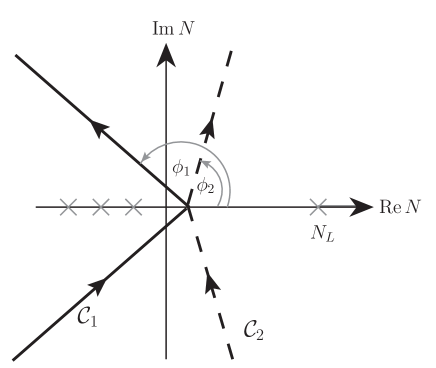
Figure 3: The two contours in Mellin-$N$ space for inverting the product of moments of the resummed partonic cross sections and the fragmentation functions. The crosses symbolize the poles of the fragmentation functions and LO cross sections on the real axis. $N_{L}$ is the position of the leftmost Landau pole.

Resummation takes place in Mellin-$N$ moment space, and one therefore needs an inverse Mellin transform to translate the result back into the physical space. As described in Sec. III.1 (see Eq. (20)), our approach has been to place the Mellin-$N$ transformation in between the convolutions over the parton distribution functions and the fragmentation and hard scattering functions. Therefore, the inverse Mellin transform that we need is given by

$$\sigma_{D}(x,\hat{\eta})\equiv\int_{\cal{C}}\frac{dN}{2\pi i}(x^{2})^{-N}D_{h/c}^{2N+3}(\mu_{ff})\tilde{w}^{{\mathrm{resum}},2N}(\hat{\eta}).$$ (62)

The NLL expanded forms, Eqs. (39), (40), have singularities for $\lambda=1/2$ and $\lambda=1$, known as Landau poles and corresponding to moments $N_{L}=\exp(1/(2\alpha_{s}b_{0}))$ and $N_{L}=\exp(1/(\alpha_{s}b_{0}))$, respectively, that are located on the positive real axis in moment space. Therefore a prescription has to be found for dealing with these singularities. We follow the minimal prescription Catani et al. (1996), according to which the contour for the inverse transformation runs between the first Landau pole $N_{L}$ and the rightmost of all other poles of the integrand. This choice ensures that the perturbative expansion is an asymptotic series that has no factorial divergence Catani et al. (1996). Because of the branch cuts starting at the Landau poles to the right of the contour, the inverted $\sigma_{D}(x,\hat{\eta})$ has support at $x>1$ Catani et al. (1996); Almeida et al. (2009). Although the contribution from this unphysical region decreases exponentially with $x$, we find that it is not negligible for the kinematics of interest for phenomenology, even after subsequent convolution with the parton distributions. This possibly points to significant non-perturbative effects for the cross section and kinematic regime we consider here.

For our numerical computations, we choose the inverse Mellin contours ${\cal{C}}_{1}$ (for $x<1$) and ${\cal{C}}_{2}$ (for $x>1$) illustrated in Fig. 3 in the complex-$N$ plane. Bending the contours at non-zero angles with respect to the imaginary axis improves the numerical convergence of the integrals. The contour ${\cal{C}}_{2}$ is still chosen to be rather steep, in order to avoid strong oscillations resulting from the branch cuts.

When using resummation to provide theoretical predictions of cross sections, one wants to make use of the best fixed-order theoretical calculation available, which in this case is NLO. Therefore, we “match” our resummed cross section to the NLO one. This is achieved by expanding the partonic cross sections to the first non-trivial order in $\alpha_{s}$ ($\mathcal{O}(\alpha_{s}^{2})$ for the direct case, $\mathcal{O}(\alpha_{s}^{3})$ for the resolved one), subtracting the expanded result from the resummed one, and adding the full NLO cross section:

$$\frac{p_{T}^{3}d\sigma^{{\mathrm{matched}}}}{dp_{T}d\eta}=\sum_{a,b,c}\int_{0}^{1}dx_{\ell}\int_{0}^{1}dx_{n}$$

$$\times f_{a/\ell}(x_{\ell},\mu_{fi})f_{b/N}(x_{n},\mu_{fi})$$

$$\times\int_{\cal{C}}\frac{dN}{2\pi i}(x^{2})^{-N}D_{h/c}^{2N+3}(\mu_{ff})$$

$$\times\left[\tilde{w}^{{\mathrm{resum}},2N}_{ab\rightarrow cd}(\hat{\eta})-\left.\tilde{w}^{{\mathrm{resum}},2N}_{ab\rightarrow cd}(\hat{\eta})\right|_{{\mathrm{first-order}}}\right]$$

$$+\frac{p_{T}^{3}d\sigma^{{\mathrm{NLO}}}}{dp_{T}d\eta}.$$ (63)

This procedure allows to take into account the NLO calculation in full. The soft-gluon contributions beyond NLO are resummed to NLL.

IV Phenomenological Results

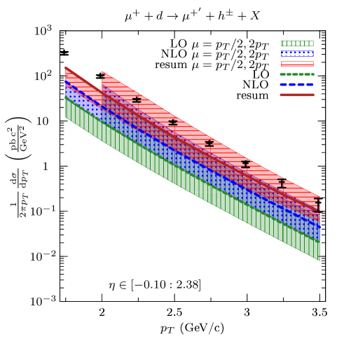
Figure 4: Comparison of the LO, NLO and resummed (“resum”) calculations to COMPASS data. The error bars shown for the experimental data are the quadratic sums of statistical and systematic uncertainties. In addition, there is a 10% normalization uncertainty due to the luminosity determination. For scale $\mu=p_{T}/2$ we only show results for $p_{T}\geq 2\,$GeV.

Starting from Eq. (63) we now compare the resummed cross section to experimental hadron production data measured at the COMPASS experiment at CERN Adolph et al. (2012). In this fixed-target experiment muons at a beam energy of $E_{\mu}=160\,$GeV were scattered off a deuteron target, corresponding to a lepton-nucleon center-of-mass energy of $\sqrt{s}=17.4\,$GeV. Due to a detector area cut the fraction $y$ of the lepton momentum carried by the photon is restricted to the range $0.2\leq y\leq 0.8$. For the COMPASS photoproduction studies the maximally allowed virtuality $Q^{2}_{{\mathrm{max}}}$ of the photons was $Q^{2}_{{\mathrm{max}}}=0.1\,{\rm GeV}^{2}$. The measured hadrons $h^{\pm}$ were subject to the following kinematic cuts: the fraction $z_{{\mathrm{cut}}}$ of the virtual photon energy carried by the detected hadron had to be within the range $0.2\leq z_{{\mathrm{cut}}}\leq 0.8$. In addition, the scattering angle $\theta$ of the observed hadron was constrained by $10\leq\theta\leq 120\,$mrad, corresponding to $2.38\geq\eta\geq-0.1$ in pseudo-rapidity in the lepton-nucleon center-of-mass system.

In our calculations we use the CTEQ6M5 set of parton distribution functions for the nucleon Tung et al. (2007) and the “Glück-Reya-Schienbein” (GRS) parton distribution functions of the photon Glück et al. (1999). For the fragmentation functions we use the “de Florian-Sassot-Stratmann” (DSS) set de Florian et al. (2007). All scales in Eq. (63) are set equal, $\mu=\mu_{r}=\mu_{fi}=\mu_{ff}=p_{T}$. In order to investigate the scale dependence of our results, we will also show the results for $\mu=p_{T}/2$ and $\mu=2p_{T}$.

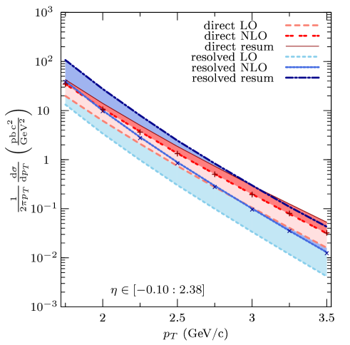
Figure 5: The direct contribution versus the resolved one in the $\overline{\text{MS}}$ scheme for the photon’s parton distributions. The crosses denote the first-order expansions of the direct and resolved resummed cross sections.

Figure 6: Soft-gluon “$K$-factors” relative to NLO, as defined in Eq. (64), for COMPASS kinematics. The numbers labeling the curves refer to the superscript $n$ in $K^{(n)}$ in Eq. (64).

In Fig. 4 we present our results for the matched resummed cross section for photoproduction in $\mu d\to h^{\pm}X$ for COMPASS kinematics and compare it to the experimental data Adolph et al. (2012). Note that the data are available down to low transverse momentum $p_{T}=1.2\,$GeV, while we start our theoretical cross sections at $p_{T}=1.75\,$GeV to make sure that application of perturbative methods is sensible. For all our calculations we have applied the cuts on the momentum fraction $y$ in the Weizsäcker-Williams photon and on the photon’s maximal virtuality given above. Moreover, thanks to our rapidity-dependent resummed approach, we are able to take into account the proper pseudo-rapidity cuts $2.38\geq\eta\geq-0.1$ as well as $0.2\leq z_{{\mathrm{cut}}}\leq 0.8$ directly. Fig. 4 also shows the LO and the NLO cross section. One observes that the LO one is far below the data. The NLO corrections are huge, which indicates the importance of going beyond NLO and taking into account the threshold logarithms to all orders. The matched resummed cross section gives again a sizeable correction to the NLO result, enhancing the latter by a factor of about two. One observes that the resummed results agree with the data within the (admittedly, large) systematic error. Note that unfortunately for the kinematics discussed here the scale uncertainty of the resummed result is not really smaller than that of the LO or the NLO one.

Even if neither the direct contribution $d\sigma_{{\mathrm{dir}}}$ nor the resolved one $d\sigma_{{\mathrm{res}}}$ are individually measurable quantities as both of them depend on the scheme chosen for the factorization of singular collinear parton emissions, it is instructive to consider both parts separately. The direct processes will generally dominate at high $p_{T}$. On the other hand, in contrast to the direct processes, the resolved ones have an additional intermediate particle generated by the photon. As this carries only a fraction $x_{\gamma}$ of the photon momentum, less phase space is available for producing a high-momentum hadron. Therefore the resolved processes are on average closer to the partonic threshold, and thus we expect the threshold logarithms to have more impact than for the direct contribution. In addition, the resolved processes involve four colored partons, making them more likely to radiate soft gluons. Fig. 5 compares the direct and resolved contributions and the resummation effects on them. At lowest order the direct contribution exceeds the resolved one over the whole $p_{T}$-range considered. This changes already at NLO: Because of the large size of the NLO corrections in the resolved case, the resolved NLO cross section exceeds the direct NLO one at $p_{T}\leq 2\,$GeV. This trend continues for the resummed cross sections.

In order to see whether the large effects from soft-gluon resummation correctly give the dominant part of the cross section, we perform a consistency check. For each subprocess the resummed cross section (not the matched one) is expanded to NLO and compared to the corresponding full fixed-order NLO result. We find that these expansions reproduce the NLO results very well for all processes, except for $gg\rightarrow q\bar{q}$ which, however, only makes a small contribution to the full cross section. We have not been able to identify the reason for the discrepancy in this particular case, except that we found that it is due to terms not related to “+”-distributions. Figure  5 also shows these comparisons, again separately for the direct and resolved contributions, where for each of the two we have combined all relevant subprocesses. As can be observed, the agreement of the expansion and the NLO result is excellent. This implies that the terms that are formally suppressed by an inverse power of the Mellin moment $N$ near threshold indeed are insignificant. Thus one may safely assume that this will also be the case for higher-order corrections, so that the resummed cross section yields a good approximation to the all-order perturbative cross section.

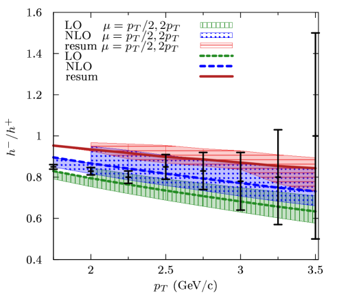
Figure 7: Ratio of production cross sections for $h^{-}$ over $h^{+}$: $d\sigma_{\mu^{+}d\rightarrow\mu^{+^{\prime}}+h^{-}}/d\sigma_{\mu^{+}d\rightarrow\mu^{+^{\prime}}+h^{+}}$. The error bars of the experimental data are statistical only.

Figure 8: Ratios of the $y$-dependent resummed and NLO cross sections, integrated over various $p_{T}$ bins. The cross sections are averaged over the ranges $[y-0.05:y+0.05]$.

We now investigate how the large enhancement of the NLL resummed cross section that we observed in Fig. 4 builds up order by order. We therefore expand the matched resummed formula beyond NLO and define the “soft-gluon $K$-factors”

$$K^{(n)}\equiv\frac{\left.d\sigma^{{\mathrm{matched}}}/dp_{T}\right|_{\mathcal{O}(\alpha_{s}^{1+n})}}{d\sigma^{{\mathrm{NLO}}}/dp_{T}}.$$ (64)

In addition, $K^{{\mathrm{resum}}}\equiv K^{(\infty)}$ is defined as the ratio of the matched resummed cross section to the NLO one. Because of the matching procedure given by Eq. (63), the first-order expansion of the matched resummed cross section is identical to the full fixed order NLO result, and we have $K^{(1)}=1$. Figure  6 shows $K^{{\mathrm{resum}}}$ along with the six lowest soft-gluon $K$-factors. One can see that they are almost flat for $p_{T}\leq 3.5\,$GeV but exhibit a dramatic enhancement for higher transverse momenta. Figure  6 also indicates that the series $K^{(1)},K^{(2)},K^{(3)}\ldots$ converges towards $K^{{\mathrm{resum}}}$, which may be regarded as further evidence for the importance of resummation.

Next, we study the ratio of the production cross section for negatively charged hadrons over the one for positively charged hadrons. This ratio is also accessible at COMPASS. Figure  7 shows our calculation compared to the data. As expected, the production of positively charged mesons is preferred. This effect mostly stems from the QCD-Compton process $\gamma q\to qg$ in the direct channel which couples to up quarks four times as strongly as to down quarks. This tendency is most distinct for LO and softens when going to NLO and to the NLL resummed cross section, since resolved higher-order contributions are gaining importance. Figure  7 shows that the resummed cross section somewhat overpredicts the charge ratio measured in experiment. We note, however, that we have obtained the scale uncertainty bands in the figure by simply dividing the $h^{-}$ and $h^{+}$ cross sections for a given scale. The true scale uncertainty on the ratio will likely be larger as one could, in principle, choose different scales in the computation of the two cross sections.

Finally, in Fig. 8 we investigate the dependence of the cross section on the photon energy fraction $y$ in the Weizsäcker-Williams spectrum. We consider the double differential cross section $d^{2}\sigma/(dp_{T}dy)$ integrated over $p_{T}$ bins and averaged over the ranges $[y-0.05:y+0.05]$,

$$\frac{1}{0.1}\int_{y-0.05}^{y+0.05}dy^{\prime}\int_{p_{T},a}^{p_{T},b}\frac{d^{2}\sigma}{dp_{T}dy^{\prime}}dp_{T}.$$ (65)

At fixed transverse momentum the phase space available for the production of additional partons is smaller, the smaller the photon energy fraction $y$. Therefore, for decreasing $y$ one gets closer to partonic threshold, and one expects an increase of the cross section due to the impact of soft gluon emissions. This behavior is more pronounced at higher $p_{T}$. As $y$ is directly accessible in experiment, the $y$-dependence of the cross section may give information about whether hadron production at this kinematics is well-described by perturbative methods.

V Conclusions

We have studied the effects of next-to-leading logarithmic threshold logarithms on the direct- and resolved-photon cross sections for the process $\mu^{+}d\rightarrow\mu^{+^{\prime}}+h+X$ at high transverse momentum of the hadron $h$. As a new technical ingredient to resummation, we were able to fully include the rapidity dependence of the cross section in the resummed calculation and to account for all relevant experimental cuts. This was achieved by treating only the partonic cross sections and the fragmentation functions in Mellin-$N$ moment space, but keeping the convolutions with the parton distribution functions in $x$-space.

For COMPASS kinematics, we have found large higher-order soft-gluon QCD corrections. These are due to the fact that one is overall rather close to the threshold region, as shown by the relatively large value of the hadron’s transverse momentum over the available center-of-mass energy, typically $2p_{T}/\sqrt{s}\gtrsim 0.1$. The threshold logarithms addressed by resummation strongly dominate the higher-order corrections. We have verified this by comparing the first-order expansion of our resummed cross section with the full NLO one, finding excellent agreement of the two. We have observed a significant enhancement of the resummed cross section over the next-to-leading order one, showing that the NLO calculations are likely not fully sufficient. Resummation also significantly improves the agreement between the data and theoretical predictions. It will be interesting to extend our calculations to the case of helicity asymmetries for this process, which are used at COMPASS to access the nucleon’s spin-dependent gluon distribution.