Non-linear Dimensionality Reduction: Riemannian Metric Estimation and the Problem of Geometric Recovery

Abstract

In recent years, manifold learning has become increasingly popular as a tool for performing non-linear dimensionality reduction. This has led to the development of numerous algorithms of varying degrees of complexity that aim to recover manifold geometry using either local or global features of the data.

Building on the Laplacian Eigenmap and Diffusionmaps framework, we propose a new paradigm that offers a guarantee, under reasonable assumptions, that any manifold learning algorithm will preserve the geometry of a data set. Our approach is based on augmenting the output of embedding algorithms with geometric information embodied in the Riemannian metric of the manifold. We provide an algorithm for estimating the Riemannian metric from data and demonstrate possible applications of our approach in a variety of examples.

1 Introduction

When working with large sets of high-dimensional data, one is regularly confronted with the problem of tractability and interpretability of the data. An appealing approach to this problem is the method of dimensionality reduction: finding a low-dimensional representation of the data that preserves all or most of the important “information”. One popular idea for Euclidean data is to appeal to the manifold hypothesis, whereby the data is assumed to lie on a low-dimensional smooth manifold embedded in the high dimensional space. The task then becomes to recover the low-dimensional manifold so as to perform any statistical analysis on the lower dimensional representation of the data.

A common technique for performing dimensionality reduction is Principal Component Analysis, which assumes that the low-dimenisional manifold is an affine space. The affine space requirement is generally violated in practice and this has led to the development of more general techniques which perform non-linear dimensionality reduction. Although not all non-linear dimensionality reduction techniques are based on the manifold hypothesis, manifold learning has been a very popular approach to the problem. This is in large part due to the easy interpretability and mathematical elegance of the manifold hypothesis.

The popularity of manifold learning has led to the development of numerous algorithms that aim to recover the geometry of the low-dimensional manifold $\mathcal{M}$ using either local or global features of the data. These algorithms are of varying degrees of complexity, but all have important shortcomings that have been documented in the literature (Goldberg et al., 2008; Wittman, 2005, retrieved 2010). Two important criticisms are that 1) the algorithms fail to recover the geometry of the manifold in many instances and 2) no coherent framework yet exists in which the multitude of existing algorithms can easily be compared and selected for a given application.

It is customary to evaluate embedding algorithms by how well they “recover the geometry”, i.e. preserve the important information of the data manifold, and much effort has been devoted to finding embedding algorithms that do so. While there is no uniformly accepted definition of what it means to “recover the geometry” of the data, we give this criterion a mathematical interpretation, using the concepts of Riemannian metric and isometry. The criticisms noted above reflect the fact that the majority of manifold learning algorithms output embeddings that are not isometric to the original data except in special cases.

Assuming that recovering the geometry of the data is an important goal, we offer a new perspective: rather than contributing yet another embedding algorithm that strives to achieve isometry, we provide a way to augment any reasonable embedding so as to allow for the correct computation of geometric values of interest in the embedding’s own coordinates.

The information necessary for reconstructing the geometry of the manifold is embodied in its Riemannian metric, defined in Section 4. We propose to recover a Riemannian manifold $(\mathcal{M},g)$ from the data, that is, a manifold and its Riemannian metric $g$, and express $g$ in any desired coordinate system. Practically, for any given mapping produced by an existing manifold learning algorithm, we will add an estimation of the Riemannian metric $g$ in the new data coordinates, that makes the geometrical quantities like distances and angles of the mapped data (approximately) equal to their original values, in the raw data.

We start with a brief discussion of the literature and an introduction to the Riemannian metric in Sections 2 and  3. The core of our paper is the demonstration of how to obtain the Riemannian metric from the mathematical, algorithmic and statistical points of view. These are presented in Sections 4 and 5. Finally, we offer some examples and applications in Section 6 and conclude with a discussion in Section 7.

2 The Task of Manifold Learning

In this section, we present the problem of manifold learning. We focus on formulating coherently and explicitly a two properties that cause a manifold learning algorithm to “work well”, or have intuitively desirable properties.

The first desirable property is that the algorithm produces a smooth map, and Section 3 defines this concept in differential geometry terms. This property is common to a large number of algorithms, so it will be treated as an assumption in later sections.

The second property is the preservation of the intrinsic geometry of the manifold. This property is of central interest to this article.

We begin our survey of manifold learning algorithms by discussing a well-known method for linear dimensionality reduction: Principal Component Analysis. PCA is a simple but very powerful technique that projects data onto a linear space of a fixed dimension that explains the highest proportion of variability in the data. It does so by performing an eigendecomposition of the data correlation matrix and selecting the eigenvectors with the largest eigenvalues, i.e. those that explain the most variation. Since the projection of the data is linear by construction, PCA cannot recover any curvature present in the data.

In contrast to linear techniques, manifold learning algorithms assume that the data lies near or along a non-linear, smooth, submanifold of dimension $d$ called the data manifold $\mathcal{M}$, embedded in the original high-dimensional space ${\mathbb{R}}^{r}$ with $d\ll r$, and attempt to uncover this low-dimensional ${\mathcal{M}}$. If they succeed in doing so, then each high-dimensional observation can accurately be described by a small number of parameters, its embedding coordinates $f(p)$ for all $p\in\mathcal{M}$.

Thus, generally speaking, a manifold learning or manifold embedding algorithm is a method of non-linear dimension reduction. Its input is a set of points $\mathcal{P}=\{p_{1},\ldots p_{n}\}\subset{\mathbb{R}}^{r}$, where $r$ is typically high. These are assumed to be sampled from a low-dimensional manifold $\mathcal{M}\subset{\mathbb{R}}^{r}$ and are mapped into vectors $\{f(p_{1}),\ldots f(p_{n})\}\subset{\mathbb{R}}^{s}$, with $s\ll r$ and $d\leq s$. This terminology, as well as other differential geometry terms used in this section, will later be defined formally.

2.1 Nearest Neighbors Graph

Existing manifold learning algorithms pre-process the data by first constructing a neighborhood graph $\mathcal{G}=(V,E)$, where $V$ are the vertices and $E$ the edges of $\mathcal{G}$. While the vertices are generally taken to be the observed points $V=\{p_{1},\dots,p_{n}\}$, there are three common approaches for constructing the edges.

The first approach is to construct the edges by connecting the $k$ nearest neighbors for each vertex. Specifically, $(p_{i},p_{j})\in E_{k}$ if $p_{i}$ is one of the k-nearest neighbors of $p_{j}$ or if $p_{j}$ is one of the k-nearest neighbors of $p_{i}$. $\mathcal{G}_{k}=(V,E_{k})$ is then known as the $k-$nearest neighbors graph. While it may be relatively easy to choose the neighborhood parameter $k$ with this method, it is not very intuitive in a geometric sense.

The second approach is to construct the edges by finding all the neighborhoods of radius $\sqrt{\epsilon}$ so that $E_{\epsilon}=\{\mathbf{1}[||p_{i}-p_{j}||^{2}\leq\epsilon]:i,j=1,\dots,n\}$. This is known as the $\epsilon$-neighborhood graph $\mathcal{G}_{\epsilon}=(V,E_{\epsilon})$. The advantage of this method is that it is geometrically motivated; however, it can be difficult to choose $\sqrt{\epsilon}$, the bandwidth parameter. Choosing a $\sqrt{\epsilon}$ that is too small may lead to disconnected components, while choosing a $\sqrt{\epsilon}$ that is too large fails to provide locality information - indeed, in the extreme limit, we obtain a complete graph. Unfortunately, this does not mean that the range of values between these two extremes necessarily constitutes an appropriate middle ground for any given learning task.

The third approach is to construct a complete weighted graph where the weights represent the closeness or similarity between points. A popular approach for constructing the weights, and the one we will be using here, relies on kernels Ting et al. (2010). For example, weights defined by the heat kernel are given by

$$w_{\epsilon}(i,j)=\exp{\left(\frac{-\left|\left|p_{i}-p_{j}\right|\right|^{2}}{\epsilon}\right)}$$ (1)

such that $E_{w_{\epsilon}}=\{w_{\epsilon}(i,j):i,j=1,\dots,n\}$. The weighted neighborhood graph $G_{w_{\epsilon}}$ has the same advantage as the $\epsilon$-neighborhood graph in that it is geometrically motivated; however, it can be difficult to work with given that any computations have to be performed on a complete graph. This computational complexity can partially be alleviated by truncating for very small values of $w$ (or, equivalently, for a large multiple of $\sqrt{\epsilon}$), but not without reinstating the risk of generating disconnected components. However, using a truncated weighted neighborhood graph compares favorably with using an $\epsilon^{\prime}$-neighborhood graph with large values of $\epsilon^{\prime}$ since the truncated weighted neighborhood graph $G_{w_{\epsilon}}$ - with $\epsilon<\epsilon^{\prime}$ - preserves locality information through the assigned weights.

In closing, we note that some authors distinguish between the step of creating the nearest neighbors graph using any one of the methods we discussed above, and the step of creating the similarity graph (Belkin and Niyogi (2002)). In practical terms, this means that one can improve on the $k$ nearest neighbors graph by applying the heat kernel on the existing edges, generating a weighted $k$ nearest neighbors graph.

2.2 Existing Algorithms

Without attempting to give a thorough overview of the existing manifold learning algorithms, we discuss two main categories. One category uses only local information, embodied in $\mathcal{G}$ to construct the embedding. Local Linear Embedding (LLE) (Saul and Roweis (2003)), Laplacian Eigenmaps (LE) (Belkin and Niyogi (2002)), Diffusion Maps (DM) (Coifman and Lafon (2006)), and Local Tangent Space Alignment (LTSA) (Zhang and Zha (2004)) are in this category.

Another approach is to use global information to construct the embedding, and the foremost example in this category is Isomap (Tenenbaum et al. (2000)). Isomap estimates the shortest path in the neighborhood graph $\mathcal{G}$ between every pair of data points $p,p^{\prime}$, then uses the Euclidean Multidimensional Scaling (MDS) algorithm (Borg and Groenen (2005)) to embed the points in $s$ dimensions with minimum distance distortion all at once.

We now provide a short overview of each of these algorithms.

• LLE: Local Linear Embedding is one of the algorithms that constructs $\mathcal{G}$ by connecting the $k$ nearest neighbors of each point. In addition, it assumes that the data is linear in each neighborhood $\mathcal{G}$, which means that any point $p$ can be approximated by a weighted average of its neighbors. The algorithm finds weights that minimize the cost of representing the point by its neighbors under the $L_{2}$-norm. Then, the lower dimensional representation of the data is achieved by a map of a fixed dimension that minimizes the cost, again under the $L_{2}$-norm, of representing the mapped points by their neighbors using the weights found in the first step.

• LE: The Laplacian Eigenmap is based on the random walk graph Laplacian, henceforth referred to as graph Laplacian, defined formally in Section 5 below. The graph Laplacian is used because its eigendecomposition can be shown to preserve local distances while maximizing the smoothness of the embedding. Thus, the LE embedding is obtained simply by keeping the first $s$ eigenvectors of the graph Laplacian in order of ascending eigenvalues. The first eigenvector is omitted, since it is necessarily constant and hence non-informative.

• DM: The Diffusion Map is a variation of the LE that emphasizes the deep connection between the graph Laplacian and heat diffusion on manifolds. The central idea remains to embed the data using an eigendecomposition of the graph Laplacian. However, DM defines an entire family of graph Laplacians, all of which correspond to different diffusion processes on $\mathcal{M}$ in the continuous limit. Thus, the DM can be used to construct a graph Laplacian whose asymptotic limit is the Laplace-Beltrami operator, defined in (4), independently of the sampling distribution of the data. This is the most important aspect of DM for our purposes.

• LTSA: The Linear Tangent Space Alignment algorithm, as its name implies, is based on estimating the tangent planes of the manifold $\mathcal{M}$ at each point in the data set using the $k$-nearest neighborhood graph $\mathcal{G}$ as a window to decide which points should be used in evaluating the tangent plane. This estimation is acheived by performing a singular value decomposition of the data matrix for the neighborhoods, which offers a low-dimensional parameterization of the tangent planes. The tangent planes are then pieced together so as to minimize the reconstruction error, and this defines a global low-dimensional parametrization of the manifold provided it can be embedded in ${\mathbb{R}}^{d}$. One aspect of the LTSA is worth mentioning here even though we will not make use of it: by obtaining a parameterization of all the tangent planes, LTSA effectively obtains the Jacobian between the manifold and the embedding at each point. This provides a natural way to move between the embedding $f(\mathcal{M})$ and $\mathcal{M}$. Unfortunately, this is not true for all embedding algorithms: more often then not, the inverse map for out-of-sample points is not easy to infer.

• MVU: Maximum Variance Unfolding (also known as Semi-Definite Embedding) (Weinberger and Saul (2006)) represents the input and output data in terms of Gram matrices. The idea is to maximize the output variance, subject to exactly preserving the distances between neighbors. This objective can be expressed as a semi-definite program.

• ISOMAP: This is an example of a non-linear global algorithm. The idea is to embed $\mathcal{M}$ in ${\mathbb{R}}^{s}$ using the minimizing geodesics between points. The algorithm first constructs $\mathcal{G}$ by connecting the $k$ nearest neighbors of each point and computes the distance between neighbors. Dijkstra’s algorithm is then applied to the resulting local distance graph in order to approximate the minimizing geodesics between each pair of points. The final step consists in embedding the data using Multidimensional Scaling (MDS) on the computed geodesics between points. Thus, even though Isomap uses the linear MDS algorithm to embed the data, it is able to account for the non-linear nature of the manifold by applying MDS to the minimizing geodesics.

• MDS: For the sake of completeness, and to aid in understanding the Isomap, we also provide a short description of MDS. MDS is a spectral method that finds an embedding into ${\mathbb{R}}^{s}$ using dissimilarities (generally distances) between data points. Although there is more than one flavor of MDS, they all revolve around minimizing an objective function based on the difference between the dissimilarities and the distances computed from the resulting embedding.

2.3 Manifolds, Coordinate Charts and Smooth Embeddings

Now that we have explained the task of manifold learning in general terms and presented the most common embedding algorithms, we focus on formally defining manifolds, coordinate charts and smooth embeddings. These formal definitions set the foundation for the methods we will introduce in Sections 3 and 4, as well as in later sections.

We first consider the geometric problem of manifold and metric representation, and define a smooth manifold in terms of coordinate charts.

Definition 1 (Smooth Manifold with Boundary )

A $d$-dimensional manifold $\mathcal{M}$ with boundary is a topological (Hausdorff) space such that every point has a neighborhood homeomorphic to an open subset of $\mathbb{H}^{d}\equiv\{(x^{1},...,x^{d})\in{\mathbb{R}}^{d}|x^{1}\geq 0\}$. A chart $(U,x)$, or coordinate chart, of manifold $\mathcal{M}$ is an open set $U\subset\mathcal{M}$ together with a homeomorphism $x:U\rightarrow V$ of $U$ onto an open subset $V\subset\mathbb{H}^{d}$. A $C^{\infty}$-Atlas $\mathcal{A}$ is a collection of charts,

$$\mathcal{A}\equiv\cup_{\alpha\in I}\{(U_{\alpha},x_{\alpha})\}\,,$$

where $I$ is an index set, such that $\mathcal{M}=\cup_{\alpha\in I}U_{\alpha}$ and for any $\alpha,\beta\in I$ the corresponding transition map,

$$x_{\beta}\circ x_{\alpha}^{-1}:x_{\alpha}(U_{\alpha}\cap U_{\beta})\rightarrow{\mathbb{R}}^{d}\,,$$ (2)

is continuously differentiable any number of times. Finally, a smooth manifold $\mathcal{M}$ with boundary is a manifold with boundary with a $C^{\infty}$-Atlas.

Note that to define a manifold without boundary, it suffices to replace $\mathbb{H}^{d}$ with ${\mathbb{R}}^{d}$ in Definition 1 . For simplicity, we assume throughout that the manifold is smooth, but it is commonly sufficient to have a $\mathcal{C}^{2}$ manifold, i.e. a manifold along with a $\mathcal{C}^{2}$ atlas. Following Lee (2003), we will identify local coordinates of an open set $U\subset\mathcal{M}$ by the image coordinate chart homeomorphism. That is, we will identify $U$ by $x(U)$ and the coordinates of point $p\in U$ by $x(p)=(x^{1}(p),...,x^{d}(p))$.

This definition allows us to reformulate the goal of manifold learning: assuming that our (high-dimensional) data set $\mathcal{P}=\{p_{1},\ldots p_{n}\}\subset{\mathbb{R}}^{r}$ comes from a smooth manifold with low $d$, the goal of manifold learning is to find a corresponding collection of $d$-dimensional coordinate charts for these data.

The definition also hints at two other well-known facts. First, the coordinate chart(s) are not uniquely defined, and there are infinitely many atlases for the same manifold $\mathcal{M}$ (Lee (2003)). Thus, it is not obvious from coordinates alone whether two atlases represent the same manifold or not. In particular, to compare the outputs of a manifold learning algorithm with the original data, or with the result of another algorithm on the same data, one must resort to intrinsic, coordinate-independent quantities. As we shall see later in this chapter, the framework we propose takes this observation into account.

The second remark is that a manifold cannot be represented in general by a global coordinate chart. For instance, the sphere is a 2-dimensional manifold that cannot be mapped homeomorphically to ${\mathbb{R}}^{2}$; one needs at least two coordinate charts to cover the 2-sphere. It is also evident that the sphere is naturally embedded in ${\mathbb{R}}^{3}$.

One can generally circumvent the need for multiple charts by mapping the data into $s>d$ dimensions as in this example. Mathematically, the grounds for this important fact are centered on the concept of embedding, which we introduce next.

Let $\mathcal{M}$ and $\mathcal{N}$ be two manifolds, and $f:\mathcal{M}\rightarrow\mathcal{N}$ be a $C^{\infty}$ (i.e smooth) map between them. Then, at each point $p\in\mathcal{M}$, the Jacobian $df_{p}$ of $f$ at $p$ defines a linear mapping between the tangent plane to $\mathcal{M}$ at $p$, denoted $T_{p}(\mathcal{M})$, and the tangent plane to $\mathcal{N}$ at $f(p)$, denoted $T_{f(p)}(\mathcal{N})$.

Definition 2 (Rank of a Smooth Map)

A smooth map $f:\mathcal{M}\rightarrow\mathcal{N}$ has rank $k$ if the Jacobian $df_{p}:T_{p}\mathcal{M}\rightarrow T_{f(p)}\mathcal{N}$ of the map has rank $k$ for all points $p\in\mathcal{M}$. Then we write $rank\left(f\right)=k$.

Definition 3 (Embedding )

Let $\mathcal{M}$ and $\mathcal{N}$ be smooth manifolds and let $f:\mathcal{M}\rightarrow\mathcal{N}$ be a smooth injective map with $rank(f)=dim(\mathcal{M})$, then $f$ is called an immersion. If $f$ is a homeomorphism onto its image, then $f$ is an embedding of $\mathcal{M}$ into $\mathcal{N}$.

The Strong Whitney Embedding Theorem (Lee (2003)) states that any $d$-dimensional smooth manifold can be embedded into ${\mathbb{R}}^{2d}$. It follows from this fundamental result that if the intrinsic dimension $d$ of the data manifold is small compared to the observed data dimension $r$, then very significant dimension reductions can be achieved, namely from $r$ to $s\leq 2d$ with a single map $f:\mathcal{M}\rightarrow{\mathbb{R}}^{s}$.

Whitney’s result is tight, in the sense that some manifolds, such as real projective spaces, need all $2d$ dimensions. However, the $r=2d$ upper bound is probably pessimistic for most data sets. Even so, the important point is that the existence of an embedding of $\mathcal{M}$ into ${\mathbb{R}}^{d}$ cannot be relied upon; at the same time, finding the optimal $s$ for an unknown manifold might be more trouble than it is worth if the dimensionality reduction from the original data is already significant, i.e. $2d\ll r$.

In light of these arguments, for the purposes of our work, we set the objective of manifold learning to be the recovery of an embedding of $\mathcal{M}$ into ${\mathbb{R}}^{s}$ subject to $d\leq s\leq 2d$ and with the additional assumption that $s$ is sufficiently large to allow a smooth embedding. That being said, the choice of $s$ will only be discussed tangentially in this article and even then, the constraint $s\leq 2d$ will not be enforced.

Original data	LE	LLE
$r=3$	$s=2$	$s=3$
LTSA	Isomap $k=12$	Isomap $k=8$
$s=2$	$s=2$	$s=2$

Figure 1: Manifold learning algorithms distort the geometry of the data. The classical “Swiss roll” example is shown here embedded via a variety of manifold learning algorithms. For clarity, the original data is in $r=3$ dimensions; it is obvious that adding extra dimensions does not affect the resulting embeddings.

2.4 Consistency

The previous section defined smoothness of the embedding in the ideal, continuous case, when the “input data” covers the whole manifold $\mathcal{M}$ and the algorithm is represented by the map $f:\mathcal{M}\rightarrow\mathbb{R}^{s}$. This analysis is useful in order to define what is mathematically possible in the limit.

Naturally, we would hope that a real algorithm, on a real finite data set $\mathcal{P}$, behaves in a way similar to its continuous counterpart. In other words, as the sample size $n=|\mathcal{P}|\rightarrow\infty$, we want the output of the algorithm $f_{n}(\mathcal{P})$ to converge to the output $f(\mathcal{M})$ of the continous algorithm, irrespective of the particular sample, in a probabilistic sense. This is what is generally understood as consistency of the algorithm.

Proving consistency of various manifold-derived quantities has received considerable attention in the literature ((Bernstein et al., 2000), (von Luxburg et al., 2008)). However, the meaning of consistency in the context of manifold learning remains unclear. For example, in the case of the Isomap algorithm, the convergence proof focuses on establishing that the graph that estimates the distance between two sampled points converges to the minimizing geodesic distance on the manifold $\mathcal{M}$ (Bernstein et al. (2000)). Unfortunately, the proof does not address the question of whether the empirical embedding $f_{n}$ is consistent for $f$ or whether $f$ defines a proper embedding.

Similarly, proofs of consistency for other popular algorithms do not address these two important questions, but instead focus on showing that the linear operators underpinning the algorithms converge to the appropriate differential operators (Coifman and Lafon (2006); Hein et al. (2007); Giné and Koltchinskii (2006); Ting et al. (2010)). Although this is an important problem in itself, it still falls short of establishing that $f_{n}\rightarrow f$. The exception to this are the results in von Luxburg et al. (2008); Belkin and Niyogi (2007) that prove the convergence of the eigendecomposition of the graph Laplacian to that of the Laplace-Beltrami operator (defined in Section 4) for a uniform sampling density on $\mathcal{M}$. These results also allow us to assume, by extension, the consistency of the class of algorithms that use the eigenvectors of the Laplace-Beltrami operator to construct embeddings - Laplacian Eigenmaps and Diffusion Maps.Though incomplete in some respects, these results allow us to assume when necessary that an embedding algorithm is consistent and in the limit produces a smooth embedding.

We now turn to the next desirable property, one for which negative results abound.

2.5 Manifold Geometry Preservation

Having a consistent smooth mapping from $f:\mathcal{M}\;\rightarrow\;{\mathbb{R}}^{s}$ guarantees that neighborhoods in the high dimensional ambient space will be mapped into neighborhoods in the embedding space with some amount of “stretching”, and vice versa. A reasonable question, therefore, is whether we can reduce this amount of “stretching” to a minimum, even to zero. In other words, can we preserve not only neighborhood relations, but also distances within the manifold? Or, going one step further, could we find a way to simultaneously preserve distances, areas, volumes, angles, etc. - in a word, the intrinsic geometry - of the manifold?

Manifold learning algorithms generally fail at preserving the geometry, even in simple cases. We illustrate this with the well-known example of the “Swiss-roll with a hole” (Figure 1), a two dimensional strip with a rectangular hole, rolled up in three dimensions, sampled uniformly. Of course, no matter how the original sheet is rolled without stretching, lengths of curves within the sheet will be preserved. So will areas, angles between curves, and other geometric quantities. However, when this data set is embedded using various algorithms, this does not occur. The LTSA algorithm recovers the original strip up to an affine coordinate transformation (the strip is turned into a square); for the other algorithms, the “stretching” of the original manifold varies with the location on the manifold. As a consequence, distances, areas, angles between curves - the intrinsic geometric quantities - are not preserved between the original manifold and the embeddings produced by these algorithms.

These shortcomings have been recognized and discussed in the literature ((Goldberg et al., 2008; Zha and Zhang, 2003)). More illustrative examples can easily be generated with the software in (Wittman, 2005, retrieved 2010).

The problem of geometric distortion is central to this article: the main contribution is to offer a constructive solution to it. The definitions of the relevant concepts and the rigorous statement of the problem we will be solving is found in the next section.

We conclude this section by stressing that the consistency of an algorithm, while being a necessary property, does not help alleviate the geometric distortion problem, because it merely guarantees that the mapping from a set of points in high dimensional space to a set of points in $s$-space induced by a manifold learning algorithm converges. It will not guarantee that the mapping recovers the correct geometry of the manifold. In other words, even with infinite data, the distortions observed in Figure 1 will persist.

3 Riemannian Geometry

In this section, we will formalize what it means for an embedding $f:\mathcal{M}\rightarrow{\mathbb{R}}^{m}$ to preserve the geometry of $\mathcal{M}$.

3.1 The Riemannian Metric

The extension of Euclidean geometry to a manifold $\mathcal{M}$ is defined mathematically via the Riemannian metric.

Definition 4 (Riemannian Metric)

A Riemannian metric $g$ is a symmetric and positive definite tensor field which defines an inner product $<,>_{g}$ on the tangent space $T_{p}\mathcal{M}$ for every $p\in\mathcal{M}$.

Definition 5 (Riemannian Manifold)

A Riemannian manifold $(\mathcal{M},g)$ is a smooth manifold $\mathcal{M}$ with a Riemannian metric $g$ defined at every point $p\in\mathcal{M}$.

The inner product $<u,v>_{g}=g_{ij}u^{i}v^{j}$ (with the Einstein summation convention) for $u,v\in T_{p}\mathcal{M}$ is used to define usual geometric quantities such as the norm of a vector$||u||=\sqrt{<u,v>_{g}}$ and the angle between two vectors $\cos(\theta)=\frac{<u,v>_{g}}{||u||||v||}$. Thus, in any coordinate representation of $\mathcal{M}$, $g$ at point $p$ is represented as a $d\times d$ symmetric positive definite matrix.

The inner product $g$ also defines infinitesimal quantities such as the line element $dl^{2}=g_{ij}dx^{i}dx^{j}$ and the volume element $dV_{g}=\sqrt{\det(g)}dx^{1}\dots dx^{d}$, both expressed in local coordinate charts. The length $l$ of a curve $c:[a,b]\rightarrow\mathcal{M}$ parametrized by $t$ then becomes

$$l(c)\;=\;\int_{a}^{b}\sqrt{g_{ij}\frac{dx^{i}}{dt}\frac{dx^{j}}{dt}}dt,$$ (3)

where $(x^{1},...,x^{d})$ are the coordinates of chart $(U,\mathbf{x})$ with $c([a,b])\subset U$. Similarly, the volume of $W\subset U$ is given by

$$\text{Vol}(W)=\int_{W}\sqrt{\det(g)}dx^{1}\dots dx^{d}\,.$$ (4)

Obviously, these definitions are trivially extended to overlapping charts by means of the transition map (2). For a comprehensive treatement of calculus on manifolds, the reader is invited to consult (Lee, 1997).

3.2 Isometry and the Pushforward Metric

Having introduced the Riemannian metric, we can now formally discuss what it means for an embedding to preserve the geometry of $\mathcal{M}$.

Definition 6 (Isometry)

Let $f:\mathcal{M}\rightarrow{\cal N}$ be a diffeomorphism between two Riemannian manifolds $(\mathcal{M},g),\,({\cal N},h)$ is called an isometry iff for all $p\in\mathcal{M}$ and all $u,w\in T_{p}(\mathcal{M})$

$$<u,w>_{g(p)}\;=\;<df_{p}u,d_{p}fw>_{h(f(p))}$$

In the above, $df_{p}$ denotes the Jacobian of $f$ at $p$, i.e. the map $df_{p}:T_{p}\mathcal{M}\rightarrow T_{f(p)}\mathcal{N}$. An embedding will be isometric if $(f(\mathcal{M}),h|_{f(\mathcal{M})})$ is isometric to $(\mathcal{M},g)$, where $h|_{f(\mathcal{M})}$ is the restriction of $h$, the metric of the embedding space $\mathcal{N}$, to the tangent space $T_{f(p)}f(\mathcal{M})$. An isometric embedding obviously preserves path lengths, angles, areas and volumes. It is then natural to take isometry as the strictest notion of what it means for an algorithm to “preserve geometry”.

We also formalize what it means to carry the geometry over from a Riemannian manifold $(\mathcal{M},g)$ via an embedding $f$.

Definition 7 (Pushforward Metric)

Let $f$ be an embedding from the Riemannian manifold $(\mathcal{M},g)$ to another manifold ${\mathcal{N}}$. Then the pushforward $h=\varphi^{*}g$ of the metric $g$ along $\varphi\equiv f^{-1}$ is given by

$$\left\langle u,v\right\rangle_{\varphi^{*}g_{p}} = \left\langle df_{p}^{-1}u,df_{p}^{-1}v\right\rangle_{g_{p}}\,,$$

for $u,v\in T_{f(p)}{\mathcal{N}}$ and where $df_{p}^{-1}$ denotes the Jacobian of $f^{-1}$.

This means that, by construction, $({\mathcal{N}},h)$ is isometric to $(\mathcal{M},g)$.

As the defintion implies, the superscript $-1$ also refers to the fact that $df_{p}^{-1}$ is the matrix inverse of the jacobian $df_{p}$. This inverse is well-defined since $f$ has full rank $d$. In the next section, we will extend this definition by considering the case where $f$ is no longer full-rank.

3.3 Isometric Embedding vs. Metric Learning

Now consider a manifold embedding algorithm, like Isomap or Laplacian Eigenmaps. These algorithms take points $p\in{\mathbb{R}}^{r}$ and map them through some function $f$ into ${\mathbb{R}}^{s}$. The geometries in the two representations are given by the induced Euclidean scalar products in ${\mathbb{R}}^{r}$ and ${\mathbb{R}}^{s}$, respectively, which we will denote by $\delta_{r},\,\delta_{s}$. In matrix form, these are represented by unit matrices. In view of the previous definitions, the algorithm will preserve the geometry of the data only if the new manifold $(f(\mathcal{M}),\delta_{s})$ is isometric to the original data manifold $(\mathcal{M},\delta_{r})$.

The existence of an isometric embedding of a manifold into ${\mathbb{R}}^{s}$ for some $s$ large enough is guaranteed by Nash’s theorem ((Nash, 1956)), reproduced here for completeness.

Theorem 8

If $\mathcal{M}$ is a given $d$-dimensional Riemannian manifold of class $C^{k},\,3\leq k\leq\infty$ then there exists a number $s\leq d(3d+11)/2$ if $\mathcal{M}$ is compact, or $s\leq d(d+1)(3d+11)/2$ if $\mathcal{M}$ is not compact, and an injective map $f:\mathcal{M}\,\longrightarrow\,{\mathbb{R}}^{s}$ of class $C^{k}$, such that

$$<u,v>\,=\,<df_{p}(v),\,df_{p}(v)>$$

for all vectors $u,\,v$ in $T_{p}\mathcal{M}$.

The method developed by Nash to prove the existence of an isometric embedding is not practical when it comes to finding an isometric embedding for a data manifold. The problem is that the method involves tightly wrapping the embedding around extra dimensions, which, as observed by (Dreisigmeyer and Kirby, 2007, retrieved June 2010), may not be stable numerically.

Practically, however, as it was shown in Section 2.5, manifold learning algorithms do not generally define isometric embeddings. The popular approach to resolving this problem is to try to correct the the resulting embeddings as much as possible ((Goldberg and Ritov, 2009; Dreisigmeyer and Kirby, 2007, retrieved June 2010; Behmardi and Raich, 2010; Zha and Zhang, 2003)).

We believe that there is a more elegant solution to this problem, which is to carry the geometry over along with $f$ instead of trying to correct $f$ itself. Thus, we will take the coordinates $f$ produced by any reasonable embedding algorithm, and augment them with the appropriate (pushforward) metric $h$ that makes $(f(\mathcal{M}),h)$ isometric to the original manifold $(\mathcal{M},g)$. We call this procedure metric learning.

4 Recovering the Riemannian Metric: The Mathematics

We now establish the mathematical results that will allow us to estimate the Riemannian metric $g$ from data. The key to obtaining $g$ for any $C^{\infty}$-Atlas is the Laplace-Beltrami operator $\Delta_{\mathcal{M}}$ on $\mathcal{M}$, which we introduce below. Thereafter, we extend the solution to manifold embeddings, where the embedding dimension $s$ is, in general, greater than the dimension of $\mathcal{M}$, $d$.

4.1 The Laplace-Beltrami Operator and $g$

Definition 9 (Laplace-Beltrami Operator)

The Laplace-Beltrami operator $\Delta_{\mathcal{M}}$ acting on a twice differentiable function $f:\mathcal{M}\rightarrow{\mathbb{R}}$ is defined as $\Delta_{\mathcal{M}}f\equiv\text{div}\cdot\nabla f$.

In local coordinates, for chart $(U,x)$, the Laplace-Beltrami operator $\Delta_{\mathcal{M}}$ is expressed by means of $g$ as per Rosenberg (1997)

$$\Delta_{\mathcal{M}}f=\frac{1}{\sqrt{\det(g)}}\frac{\partial}{\partial x^{l}}\left(\sqrt{\det(g)}g^{lk}\frac{\partial}{\partial x^{k}}f\right)\,.$$ (5)

In (5), $g^{lk}$ denotes the $l,k$ component of the inverse of $g$ and Einstein summation is assumed.

The Laplace-Beltrami operator has been widely used in the context of manifold learning, and we will exploit various existing results about its properties. We will present those results when they become necessary. For more background, the reader is invited to consult Rosenberg (1997). In particular, methods for estimating $\Delta_{\mathcal{M}}$ from data exist and are well studied (Coifman and Lafon (2006); Hein et al. (2007); Belkin et al. (2009)). This makes using (5) ideally suited to recover $g$. The simple but powerful proposition below is the key to achieving this.

Proposition 10

Given a coordinate chart $(U,x)$ of a smooth Riemannian manifold $\mathcal{M}$ and $\Delta_{\mathcal{M}}$ defined on $\mathcal{M}$, then the $g(p)^{-1}$, the inverse of the Riemannian metric, or dual metric, at point $p\in U$ as expressed in local coordinates $x$, can be derived from

$$g^{ij}\;=\;\frac{1}{2}\Delta_{\mathcal{M}}\left(x^{i}-x^{i}(p)\right)\left(x^{j}-x^{j}(p)\right)|_{x^{i}=x^{i}(p),x^{j}=x^{j}(p)}$$ (6)

with $i,j=1,\dots,d$.

Proof  This follows directly from (5). Applying $\Delta_{\mathcal{M}}$ to the coordinate products of $x^{i}$ and $x^{j}$ centered at $x(p)$, i.e. $\frac{1}{2}\left(x^{i}-x^{i}(p)\right)\left(x^{j}-x^{j}(p)\right)$, and evaluating this expression at $x=x(p)$ using (5) gives

$$g^{lk}\frac{\partial{}}{\partial{x^{l}}}\left(x^{i}-x^{i}(p)\right)\times\frac{\partial{}}{\partial{x^{k}}}\left(x^{j}-x^{j}(p)\right)|_{x^{i}=x^{i}(p),x^{j}=x^{j}(p)}\;=\;g^{ij}\,,$$

since all the first order derivative terms vanish. The superscripts $i,j$ in the equation above and in (6) refer to the fact that $g^{ij}$ is the inverse, i.e. dual metric, of $g$ for coordinates $x^{i}$ and $x^{j}$.  
With all the components of $g^{-1}$known, it is straightforward to compute its inverse and obtain $g(p)$. The power of Proposition 10 resides in the fact that the coordinate chart is arbitrary. Given a coordinate chart (or embeddding, as will be shown below), one can apply the coordinate-free Laplace-Beltrami operator as in (6) to recover $g$ for that coordinate chart.

4.2 Recovering a Rank-Deficient Embedding Metric

In the previous section, we have assumed that we are given a coordinate chart $(U,x)$ for a subset of $\mathcal{M}$, and have shown how to obtain the Riemannian metric of $\mathcal{M}$ in that coordinate chart via the Laplace-Beltrami operator.

Here, we will extend the method to work with any embedding of $\mathcal{M}$. The main change will be that the embedding dimension $s$ may be larger than the manifold dimension $d$. In other words, there will be $s\geq d$ embedding coordinates for each point $p$, while $g$ is only defined for a vector space of dimension $d$. An obvious solution to this is to construct a coordinate chart around $p$ from the embedding $f$. This is often unnecessary, and in practice it is simpler to work directly from $f$ until the coordinate chart representation is actually required. In fact, once we have the correct metric for $f(\mathcal{M})$, it becomes relatively easy to construct coordinate charts for $\mathcal{M}$.

Working directly with the embedding $f$ means that at each embedded point $f_{p}$, there will be a corresponding $s\times s$ matrix $h_{p}$ defining a scalar product. The matrix $h_{p}$ will have rank $d$, and its null space will be orthogonal to the tangent space $T_{f(p)}f(\mathcal{M})$. We define $h$ so that $(f(\mathcal{M}),h)$ is isometric with $(\mathcal{M},g)$. Obviously, the tensor $h$ over $T_{f(p)}f(\mathcal{M})\bigoplus T_{f(p)}f(\mathcal{M})^{\perp}\cong{\mathbb{R}}^{s}$ that achieves this is an extension of the pushforward of the metric $g$ of $\mathcal{M}$.

Definition 11 (Embedding (Pushforward) Metric)

For all

$$u,v\in T_{f(p)}f(\mathcal{M})\bigoplus T_{f(p)}f(\mathcal{M})^{\perp},$$

the embedding pushforward metric $h$, or shortly the embedding metric, of an embedding $f$ at point $p\in\mathcal{M}$ is defined by the inner product

$$<u,v>_{h(f(p))} \equiv <df_{p}^{\dagger}\left(u\right),df_{p}^{\dagger}\left(v\right)>_{g(p)}\,,$$ (7)

where

$$df_{p}^{\dagger}:T_{f(p)}f(\mathcal{M})\bigoplus T_{f(p)}f(\mathcal{M})^{\perp}\rightarrow T_{p}\mathcal{M}$$

is the pseudoinverse of the Jacobian $df_{p}$ of $f:\mathcal{M}\rightarrow{\mathbb{R}}^{s}$

In matrix notation, with $df_{p}\equiv J$, $g\equiv G$ and $h\equiv H$, (7) becomes

$$u^{t}J^{t}HJv\;=\;u^{t}Gv$$ (8)

Hence,

$$H\;\equiv\;\left(J^{t}\right)^{\dagger}GJ^{\dagger}$$ (9)

In particular, when $\mathcal{M}\subset{\mathbb{R}}^{r}$, with the metric inherited from the ambient Euclidean space, as is often the case for manifold learning, we have that $G=\Pi^{t}I_{r}\Pi$, where $I_{r}$ is the Euclidean metric in ${\mathbb{R}}^{r}$ and $\Pi$ is the orthogonal projection of $v\in{\mathbb{R}}^{r}$ onto $T_{p}\mathcal{M}$. Hence, the embedding metric $h$ can then be expressed as

$$H(p)=\left(J^{t}\right)^{\dagger}\Pi(p)^{t}I_{r}\Pi(p)J^{\dagger}\,.$$ (10)

The constraints on $h$ mean that $h$ is symmetric semi-positive definite (positive definite on $T_{p}f(\mathcal{M})$ and null on $T_{p}f(\mathcal{M})^{\perp}$, as one would hope), rather than symmetric positive definite like $g$.

One can easily verify that $h$ satisfies the following proposition:

Proposition 12

Let $f$ be an embedding of $\mathcal{M}$ into ${\mathbb{R}}^{s}$; then $(\mathcal{M},g)$ and $(f(\mathcal{M}),h)$ are isometric, where $h$ is the embedding metric $h$ defined in Definition 11. Furthermore, $h$ is null over $T_{f(p)}f(\mathcal{M})^{\perp}$.

Proof  Let $u\in T_{p}\mathcal{M}$, then the map $df_{p}^{\dagger}\circ df_{p}:T_{p}\mathcal{M}\rightarrow T_{p}\mathcal{M}$ satisfies $df_{p}^{\dagger}\circ df_{p}(u)=u$, since $f$ has rank $d=dim(T_{p}\mathcal{M})$. So $\forall u,v\in T_{p}\mathcal{M}$ we have

$$<df_{p}(u),df_{p}(v)>_{h(f(p))}\;=\;<df_{p}^{\dagger}\circ df_{p}(u),df_{p}^{\dagger}\circ df_{p}(v)>_{g(p)}\;=\;<u,v>_{g(p)}$$ (11)

Therefore, $h$ ensures that the embedding is isometric. Moreover, the null space of the pseudoinverse is ${\rm Null}(df_{p}^{\dagger})={\rm Im}(df_{p})^{\perp}=T_{p}f\left(\mathcal{M}\right)^{\perp}$, hence $\forall u\in T_{p}f\left(\mathcal{M}\right)^{\perp}$ and $v$ arbitrary, the inner product defined by $h$ satisfies

$$<u,v>_{h(f(p))}\;=\;<df_{p}^{\dagger}\left(u\right),df_{p}^{\dagger}\left(v\right)>_{g(p)}\;=\;<0,df_{p}^{\dagger}\left(v\right)>_{g(p)}\;=\;0\,.$$ (12)

By symmetry of $h$, the same holds true if $u$ and $v$ are interchanged.  

Having shown that $h$, as defined, satisfies the desired properties, the next step is to show that it can be recovered using $\Delta_{\mathcal{M}}$, just as $g$ was in Section 4.1.

Proposition 13

Let $f$ be an embedding of $\mathcal{M}$ into ${\mathbb{R}}^{s}$, and $df$ its Jacobian. Then, the embedding metric $h(p)$ is given by the pseudoinverse of $\tilde{h}$, where

$$\tilde{h}^{ij}\;=\;\Delta_{\mathcal{M}}\frac{1}{2}\left(f^{i}-f^{i}(p)\right)\left(f^{j}-f^{j}(p)\right)|_{f^{i}=f^{i}(p),f^{j}=f^{j}(p)}$$ (13)

Proof  We express $\Delta_{\mathcal{M}}$ in a coordinate chart $(U,x)$. $\mathcal{M}$ being a smooth manifold, such a coordinate chart always exists. Applying $\Delta_{\mathcal{M}}$ to the centered product of coordinates of the embedding, i.e. $\frac{1}{2}\left(f^{i}-f^{i}(p)\right)\left(f^{j}-f^{j}(p)\right)$, then (5) means that

$$\Delta_{\mathcal{M}}\frac{1}{2}\left(f^{i}-f^{i}(p)\right)\left(f^{j}-f^{j}(p)\right)|_{f^{i}=f^{i}(p),f^{j}=f^{j}(p)} = g^{lk}\frac{\partial}{\partial x^{l}}\left(f^{i}-f^{i}(p)\right)$$

$$\times\frac{\partial}{\partial x^{k}}\left(f^{j}-f^{j}(p)\right)|_{f^{i}=f^{i}(p),f^{j}=f^{j}(p)}$$

$$= g^{kl}\frac{\partial f^{i}}{\partial x^{l}}\frac{\partial f^{j}}{\partial x^{k}}$$

Using matrix notation as before, with $J\equiv df_{p},\,G\equiv g(p),\,H\equiv h$, $\tilde{H}\equiv\tilde{h}$, the above results take the form

$$g^{kl}\frac{\partial f^{i}}{\partial x^{l}}\frac{\partial f^{j}}{\partial x^{k}}=(JG^{-1}J^{t})_{ij}=\tilde{H}_{ij}\,.$$ (14)

Hence, $\tilde{H}=JG^{-1}J^{t}$ and it remains to show that $H\;=\;\tilde{H}^{\dagger}$, i.e. that

$$\left(J^{t}\right)^{\dagger}GJ^{\dagger}=\left(JG^{-1}J^{t}\right)^{\dagger}.$$ (15)

This is obviously straightforward for square invertible matrices, but if $d<s$, this might not be the case. Hence, we need an additional technical fact: guaranteeing that

$$\left(AB\right)^{\dagger}=B^{\dagger}A^{\dagger}$$ (16)

requires $C=AB$ to constitute a full-rank decomposition of $C$, i.e. for $A$ to have full column rank and $B$ to have full row rank (Ben-Israel and Greville (2003)). In the present case, $G^{-1}$ has full rank, $J$ has full column rank, and $J^{t}$ has full row rank. All these ranks are equal to $d$ by virtue of the fact that $dim(\mathcal{M})=d$ and $f$ is an embedding of $\mathcal{M}$. Therefore, applying (16) repeatedly to $JG^{-1}J^{t}$, implicitly using the fact that $\left(G^{-1}J^{t}\right)$ has full row rank since $G^{-1}$ has full rank and $J$ has full row rank, proves that $h$ is the pseudoinverse of $\tilde{h}$.  

Discussion

Computing the pseudoinverse of $\tilde{h}$ generally means performing a Singular Value Decomposition (SVD). It is interesting to note that this decomposition offers very useful insight into the embedding. Indeed, we know from Proposition 12 that $h$ is positive definite over $T_{f(p)}f(\mathcal{M})$ and null over $T_{f(p)}f(\mathcal{M})^{\perp}$. This means that the singular vector(s) with non-zero singular value(s) of $h$ at $f(p)$ define an orthogonal basis for $T_{f(p)}f(\mathcal{M})$, while the singular vector(s) with zero singular value(s) define an orthogonal basis for $T_{f(p)}f(\mathcal{M})^{\perp}$ (not that the latter is of particular interest). Having an orthogonal basis for $T_{f(p)}f(\mathcal{M})$ provides a natural framework for constructing a coordinate chart around $p$. The simplest option is to project a small neighborhood $f(U)$ of $f(p)$ onto $T_{f(p)}f(\mathcal{M})$, a technique we will use in Section 6 to compute areas or volumes. An interesting extension of our approach would be to derive the exponential map for $f(U)$. However, computing all the geodesics of $f(U)$ is not practical unless the geodesics themselves are of interest for the application. In either case, computing $h$ allows us to achieve our set goal for manifold learning, i.e. construct a collection of coordinate charts for $\mathcal{P}$. We note that it is not always necessary, or even wise, to construct an Atlas of coordinate charts explicitly; it is really a matter of whether charts are required to perform the desired computations.

Another fortuitous consequence of computing the pseudoinverse is that the non-zero singular values yield a measure of the distortion induced by the embedding. Indeed, if the embedding were isometric to $\mathcal{M}$ with the metric inherited from ${\mathbb{R}}^{s}$, then the embedding metric $h$ would have non-zero singular values equal to 1. This can be used in many ways, such as getting a global distortion for the embedding, and hence as a tool to compare various embeddings. It can also be used to define an objective function to minimize in order to get an isometric embedding, should such an embedding be of interest. From a local perspective, it gives insight into what the embedding is doing to specific regions of the manifold and it also prescribes a simple linear transformation of the embedding $f$ that makes it locally isometric to $\mathcal{M}$ with respect to the inherited metric $\delta_{s}$. This latter attribute will be explored in more detail in Section 6.

5 Recovering the Riemannian Metric: The Algorithm

The results in the previous section apply to any embedding of $\mathcal{M}$ and can therefore be applied to the output of any embedding algorithm, leading to the estimation of the corresponding $g$ if $d=s$ or $h$ if $d<s$. In this section, we present our algorithm for the estimation procedure, called LearnMetric. Throughout, we assume that an appropriate embedding dimension $s\geq d$ is already selected and $d$ is known.

5.1 Discretized Problem

Prior to explaining our method for estimating $h$ for an embedding algorithm, it is important to discuss the discrete version of the problem.

As briefly explained in Section 2, the input data for a manifold learning algorithm is a set of points $\mathcal{P}=\{p_{1},\dots,p_{n}\}\subset\mathcal{M}$ where $\mathcal{M}$ is a compact Riemannian manifold. These points are assumed to be an i.i.d. sample with distribution $\pi$ on $\mathcal{M}$, which is absolutely continuous with respect to the Lebesgue measure on $\mathcal{M}$. From this sample, manifold learning algorithms construct a map $f_{n}:\mathcal{P}\rightarrow{\mathbb{R}}^{s}$, which, if the algorithm is consistent, will converge to an embedding $f:\mathcal{M}\rightarrow{\mathbb{R}}^{s}$.

Once the map is obtained, we go on to define the embedding metric $h_{n}$. Naturally, it is relevant to ask what it means to define the embedding metric $h_{n}$ and how one goes about constructing it. Since $f_{n}$ is defined on the set of points $\mathcal{P}$, $h_{n}$ will be defined as a positive semidefinite matrix over $\mathcal{P}$. With that in mind, we can hope to construct $h_{n}$ by discretizing equation (13). In practice, this is acheived by replacing $f$ with $f_{n}$ and $\Delta_{\mathcal{M}}$ with some discrete estimator $\tilde{\mathcal{L}}_{\epsilon,n}$ that is consistent for $\Delta_{\mathcal{M}}$.

We still need to clarify how to obtain $\tilde{\mathcal{L}}_{\epsilon,n}$. The most common approach, and the one we favor here, is to start by considering the “diffusion-like” operator $\tilde{\mathcal{D}}_{\epsilon,\lambda}$ defined via the heat kernel $w_{\epsilon}$ (see (1)):

$$\tilde{\mathcal{D}}_{\epsilon,\lambda}(f)(x) = \int_{\mathcal{M}}\frac{\tilde{w}_{\epsilon,\lambda}(x,y)}{\tilde{t}_{\epsilon,\lambda}})f(y)\pi(y)dV_{g}(y)\,,\,\,\text{with }x\in\mathcal{M}\text{ and where}$$ (17)

$$\tilde{t}_{\epsilon,\lambda}(x) = \int_{\mathcal{M}}\tilde{w}_{\epsilon,\lambda}(x,y))\pi(y)dV_{g}(y)\,,\,\,\text{and}\,\,w_{\epsilon,\lambda}=\frac{w_{\epsilon}(x,y)}{t_{\epsilon}^{\lambda}(x)t_{\epsilon}^{\lambda}(y)}\,,\,\,\text{while}$$

$$\,\,t_{\epsilon}(x) = \int_{\mathcal{M}}w_{\epsilon}(x,y)\pi(y)dV_{g}(y)\,,$$

Coifman and Lafon (2006) showed that $\tilde{\mathcal{D}}_{\epsilon,\lambda}(f)=f+\epsilon c\Delta_{\mathcal{M}}f+\mathcal{O}(\epsilon^{2})$ provided $\lambda=1$, $f\in\mathcal{C}^{3}(\mathcal{M})$, and where $c$ is a constant that depends on the choice of kernel $w_{\epsilon}$. Here, $\lambda$ is introduced to guarantee the appropriate limit in cases where the sampling density $\pi$ is not uniform on $\mathcal{M}$.

Now that we have obtained an operator that we know will converge to $\Delta_{\mathcal{M}}$, i.e.

$$\tilde{\mathcal{L}}_{\epsilon,1}(f)\equiv\frac{\tilde{\mathcal{D}}_{\epsilon,1}(f)-f}{c\epsilon}=\Delta_{\mathcal{M}}f+\mathcal{O}(\epsilon)\,,$$ (18)

we turn to the discretized problem, since we are dealing with a finite sample of points from $\mathcal{M}$.

Discretizing (17) entails using the finite sample approximation:

$$\tilde{\mathcal{D}}_{\epsilon,n}(f)(x) = \sum_{p_{i}\in\mathcal{P}}\frac{w_{\epsilon,\lambda}(x,p_{i})}{\tilde{t}_{\epsilon,\lambda,n}(x)}f(p_{i})\,,\,\,\text{with }x\in\mathcal{M}\text{ and where}$$ (19)

$$\tilde{t}_{\epsilon,\lambda,n}(x) = \sum_{p_{i}\in\mathcal{P}}\tilde{w}_{\epsilon,\lambda}(x,p_{i})\,,\,\,\text{and}\,\,\tilde{w}_{\epsilon,\lambda}=\frac{w_{\epsilon}(x,y)}{t_{\epsilon}^{\lambda}(x)d_{\epsilon}^{\lambda}(y)}\,,\,\,\text{while}$$

$$\,\,t_{\epsilon}(x) = \sum_{p_{i}\in\mathcal{P}}w_{\epsilon}(x,p_{i})\,,$$

and (18) now takes the form

$$\tilde{\mathcal{L}}_{\epsilon,n}(f)\equiv\frac{\tilde{\mathcal{D}}_{\epsilon,1}(f)-f}{c\epsilon}=\Delta_{\mathcal{M}}f+\mathcal{O}(\epsilon)\,.$$ (20)

Operator $\tilde{\mathcal{L}}_{\epsilon,n}$ is known as the geometric graph Laplacian (Zhou and Belkin (2011)). We will refer to it simply as graph Laplacian in our discussion, since it is the only type of graph Laplacian we will need.

Note that since is $\mathcal{M}$ unknown, it is not clear when $x\in\mathcal{M}$ and when $x\in{\mathbb{R}}^{r}\setminus\mathcal{M}$. The need to define $\tilde{\mathcal{L}}_{\epsilon,n}(f)$ for all $x$ in $\mathcal{M}$ is mainly to study its asymptotic properties. In practice however, we are interested in the case of $x\in\mathcal{P}$. The kernel $w_{\epsilon}(x,y)$ then takes the form of weighted neighborhood graph $\mathcal{G}_{w_{\epsilon}}$, which we denote by the weight matrix $W_{i,j}=w_{\epsilon}(p_{i},p_{j}),\,p_{i},p_{j}\in\mathcal{P}$. In fact, (19) and (20) can be expressed in terms of matrix operations when $x\in\mathcal{P}$ as done in Algorithm 1.

Algorithm 1 GraphLaplacian

  Input: Weight matrix $W$, bandwidth $\sqrt{\epsilon}$, and $\lambda$

  $D\leftarrow\text{diag}(W\mathbf{1})$

  $\tilde{W}\leftarrow D^{-\lambda}WD^{-\lambda}$

  $\tilde{D}\leftarrow\text{diag}(\tilde{W}\mathbf{1})$

  $L\leftarrow(c\epsilon)^{-1}(\tilde{D}^{-1}\tilde{W}-I_{n})$

  Return $L$

With $\tilde{\mathcal{L}}_{\epsilon,n}$, the discrete analogue to (5), clarified, we are now ready to introduce the central algorithm of this article.

5.2 The LearnMetric  Algorithm

The input data for a manifold learning algorithm is a set of points $\mathcal{P}=\{p_{1},\dots,p_{n}\}\subset\mathcal{M}$ where $\mathcal{M}$ is an unknown Riemannian manifold. Our LearnMetric  algorithm takes as input, along with dataset $\mathcal{P}$, an embedding dimension $s$ and an embedding algorithm, chosen by the user, which we will denote by GenericEmbed. LearnMetric  proceeds in four steps, the first three being preparations for the key fourth step.

1. construct a weighted neighborhood graph $\mathcal{G}_{w_{\epsilon}}$

2. calculate the graph Laplacian $\tilde{\mathcal{L}}_{\epsilon,n}$

3. map the data $p\in\mathcal{P}$ to $f_{n}(p)\in{\mathbb{R}}^{s}$ by GenericEmbed

4. apply the graph Laplacian $\tilde{\mathcal{L}}_{\epsilon,n}$ to the coordinates $f_{n}$ to obtain the embedding metric $h$

Figure 3 contains the LearnMetric  algorithm in pseudocode. The subscript $n$ in the notation indicates that these are discretized, “sample” quantities, (i.e. $f_{n}$ is a vector and $\tilde{\mathcal{L}}_{\epsilon,n}$ is a matrix) as opposed to the continuous quantities (functions, operators) that we were considering in the previous sections. We now move to describing each of the steps of the algorithm.

The first two steps, common to many manifold learning algorithms, have already been described in subsections 2.1 and 5.1 respectively. The third step calls for obtaining an embedding of the data points $p\in\mathcal{P}$ in ${\mathbb{R}}^{s}$. This can be done using any one of the many existing manifold learning algorithms (GenericEmbed), such as the Laplacian Eigenmaps, Isomap or Diffusion Maps.

At this juncture, we note that there may be overlap in the computations involved in the first three steps. Indeed, a large number of the common embedding algorithms, including Laplacian Eigenmaps, Diffusion Maps, Isomap, LLE, and LTSA use a neighborhood graph and/or similarities in order to obtain an embedding. In addition, Diffusion Maps and Eigemaps obtain an embedding for the eigendecomposition $\tilde{\mathcal{L}}_{\epsilon,n}$ or a similar operator. While we define the steps of our algorithm in their most complete form, we encourage the reader to take advantage of any efficiencies that may result from avoiding to compute the same quantities multiple times.

The fourth and final step of our algorithm consists of computing the embedding metric of the manifold in the coordinates of the chosen embedding. Step 4, applies the $n\times n$ Laplacian matrix $\tilde{\mathcal{L}}_{\epsilon,n}$ obtained in Step 2 to pairs $f^{i}_{n},\,f^{j}_{n}$ of embedding coordinates of the data obtained in Step 3. We use the symbol $\cdot$ to refer to the elementwise product between two vectors. Specfically, for two vectors $x,y\in{\mathbb{R}}^{n}$ denote by $x\cdot y$ the vector $z\in{\mathbb{R}}^{n}$ with coordinates $z=(x_{1}y_{1},\dots,x_{n}y_{n})$. This product is simply the usual function multiplication on $\mathcal{M}$ restricted to the sampled points $\mathcal{P}\subset\mathcal{M}$. Hence, equation (21) is equivalent to applying equation (13) to all the points of $p\in\mathcal{P}$ at once. The result are the vectors $\tilde{h}_{n}^{ij}$, each of which is an $n$-dimensional vector, with an entry for each $p\in\mathcal{P}$. Then, in Step 4, b, at each embedding point $f(p)$ the embedding metric $h_{n}(p)$ is computed as the matrix (pseudo) inverse of $[\tilde{h}_{n}^{ij}(p)]^{ij=1:s}$.

If the embedding dimension $s$ is larger than the manifold dimension $d$, we will obtain the rank $d$ embedding metric $h_{n}$; otherwise, we will obtain the Riemannian metric $g_{n}$. For the former, $h_{n}^{\dagger}$ will have a theoretical rank $d$, but numerically it might have rank between $d$ and $s$. As such, it is important to set to zero the $s-d$ smallest singular values of $h_{n}^{\dagger}$ when computing the pseudo-inverse. This is the key reason why $s$ and $d$ need to be known in advance. Failure to set the smallest singular values to zero will mean that $h_{n}$ will be dominated by noise. Although estimating $d$ is outside the scope of this work, it is interesting to note that the singular values of $h_{n}^{\dagger}$ may offer a window into how to do this by looking for a “singular value gap”.

In summary, the principal novelty in our LearnMetric  algorithm is its last step: the estimation of the embedding metric $h$. The embedding metric establishes a direct correspondence between geometric computations performed using $(f(\mathcal{M}),h)$ and those performed directly on $(\mathcal{M},g)$ for any embedding $f$. Thus, once augmented with their corresponding $h$, all embeddings become geometrically equivalent to each other, and to the orginal data manifold $(\mathcal{M},g)$.

Algorithm 2 PseudoInverse

  Input: Embedding metric $\tilde{h}_{n}(p)$ and intrinsic dimension $d$

  $[U,\Lambda]\leftarrow$ EigenDecomposition($\tilde{h}_{n}(p)$) where $U$ is the matrix of column eigenvectors of $\tilde{h}_{n}(p)$ ordered by their eigenvalues $\Lambda$ from largest to smallest.

  $\Lambda\leftarrow\Lambda(1:d)$ (keep $d$ largest eigenvalues)

  $\Lambda^{\dagger}\leftarrow\text{diag}(1/{\Lambda})$

  $h_{n}(p)\leftarrow U\Lambda^{\dagger}U^{t}$ (obtain rank $d$ pseudo-inverse of $\tilde{h}_{n}(p)$)

  Return $h_{n}(p)$

Algorithm 3 LearnMetric

  Input: $\mathcal{P}$ as set of $n$ data points in ${\mathbb{R}}^{r}$, $s$ the number of dimensions of the embedding, $d$ the intrinsic dimension of the manifold, $\sqrt{\epsilon}$ the bandwidth parameter, and GenericEmbed$(\mathcal{P},\,s,\sqrt{\epsilon})$ a manifold learning algorithm, that outputs $s$ dimensional embedding coordinates

1. Construct the weighted neighborhood graph with weight matrix $W$ given by $W_{i,j}=\exp{(-\frac{1}{\epsilon}||p_{i}-p_{j}^{\prime}||^{2})}$ for every points $p_{i},p_{j}\in\mathcal{P}$.

2. Construct the Laplacian matrix $\tilde{\mathcal{L}}_{\epsilon,n}$ using Algorithm 1 with input $W$, $\sqrt{\epsilon}$, and $\lambda=1$.

3. Obtain the embedding coordinates $f_{n}(p)=(f^{1}_{n}(p),\ldots,f^{s}_{n}(p))$ of each point $p\in\mathcal{P}$ by

   $$[f_{n}(p)]_{p\in\mathcal{P}}\;=\;\mbox{{\sc GenericEmbed}}(\mathcal{P},s,d,\sqrt{\epsilon})$$

4. Calculate the embedding metric $h_{n}$ for each point

   1. For $i$ and $j$ from 1 to $s$ calculate the column vector $\tilde{h}_{n}^{ij}$ of dimension $n=|\mathcal{P}|$ by

      $$\tilde{h}_{n}^{ij}\;=\;\frac{1}{2}\left[\tilde{\mathcal{L}}_{\epsilon,n}(f^{i}_{n}\cdot f^{j}_{n})-f^{i}_{n}\cdot(\tilde{\mathcal{L}}_{\epsilon,n}f^{j}_{n})-f^{j}_{n}\cdot(\tilde{\mathcal{L}}_{\epsilon,n}f^{i}_{n})\right]$$ (21)

   2. For each data point $p\in\mathcal{P}$, form the matrix $\tilde{h}_{n}(p)=[\tilde{h}_{n}^{ij}(p)]_{i,j\in{1,\dots,s}}$. The embedding metric at $p$ is then given by $h_{n}(p)=\mbox{{\sc PseudoInverse}}(\tilde{h}_{n}(p),d)$

5. Return $(f_{n}(p),h_{n}(p))_{p\in\mathcal{P}}$

5.3 Computational Complexity

Obtaining the neighborhood graph involves computing $n^{2}$ distances in $r$ dimensions. If the data is high- or very high-dimensional, which is often the case, and if the sample size is large, which is often a requirement for correct manifold recovery, this step could be by far the most computationally demanding of the algorithm. However, much work has been devoted to speeding up this task, and approximate algorithms are now available, which can run in linear time in $n$ and have very good accuracy (Ram et al. (2009)). In any event, this computationally intensive preprocessing step is required by all of the well known embedding algorithms, and would remain necessary even if one’s goal were solely to embed the data, and not to compute the Riemannian metric.

Step 2 of the algorithm operates on a sparse $n\times n$ matrix. If the neighborhood size is no larger than $k$, then it will be of order $\mathcal{O}(nk)$, and $\mathcal{O}(n^{2})$ otherwise.

The computation of the embedding in Step 3 is algorithm-dependent. For the most common algorithms, it will involve eigenvector computations. These can be performed by Arnoldi iterations that each take $\mathcal{O}(n^{2}s)$ computations, where $n$ is the sample size, and $s$ is the embedding dimension or, equivalently, the number of eigenvectors used. This step, or a variant thereof, is also a component of many embedding algorithms.

Finally, the newly introduced Step 4 involves obtaining an $s\times s$ matrix for each of the $n$ points, and computing its pseudoinverse. Obtaining the $\tilde{h}_{n}$ matrices takes $\mathcal{O}(n^{2})$ operations ($\mathcal{O}(nk)$ for sparse $\tilde{\mathcal{L}}_{\epsilon,n}$ matrix) times $s\times s$ entries, for a total of $s^{2}n^{2}$ operations. The $n$ SVD and pseudoinverse calculations take order $s^{3}$ operations.

Thus, finding the Riemannian metric makes a small contribution to the computational burden of finding the embedding. The overhead is quadratic in the data set size $n$ and embedding dimension $s$, and cubic in the intrinsic dimension $d$.

6 Experiments 

The following experiments on simulated data demonstrate the LearnMetric  algorithm and highlight a few of its immediate applications.

6.1 Embedding Metric as a Measure of Local Distortion

The first set of experiments is intended to illustrate the output of the LearnMetric  algorithm. Figure 2 shows the embedding of a 2D hourglass-shaped manifold. Diffusion Maps, the embedding algorithm we used (with $s=3$, $\lambda=1$) distorts the shape by excessively flattening the top and bottom. LearnMetric  outputs a $s\times s$ quadratic form for each point $p\in\mathcal{P}$, represented as ellipsoids centered at $p$. Practically, this means that the ellipsoids are flat along one direction $T_{f_{n}(p)}f_{n}(\mathcal{M})^{\perp}$, and two-dimensional because $d=2$, i.e. $h_{n}$ has rank 2. If the embedding correctly recovered the local geometry, $h_{n}(p)$ would equal $I_{3}|_{f_{n}(\mathcal{M})}$, the identity matrix restricted to $T_{f_{n}(p)}f_{n}(\mathcal{M})$: it would define a circle in the tangent plane of $f_{n}(\mathcal{M})$, for each $p$. We see that this is the case in the girth area of the hourglass, where the ellipses are circular. Near the top and bottom, the ellipses’ orientation and elongation points in the direction where the distortion took place and measures the amount of (local) correction needed.

The more the space is compressed in a given direction, the more elongated the embedding metric “ellipses” will be, so as to make each vector “count for more”. Inversely, the more the space is stretched, the smaller the embedding metric will be. This is illustrated in Figure 2.

Original data	Embedding with $h$ estimates
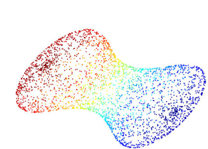
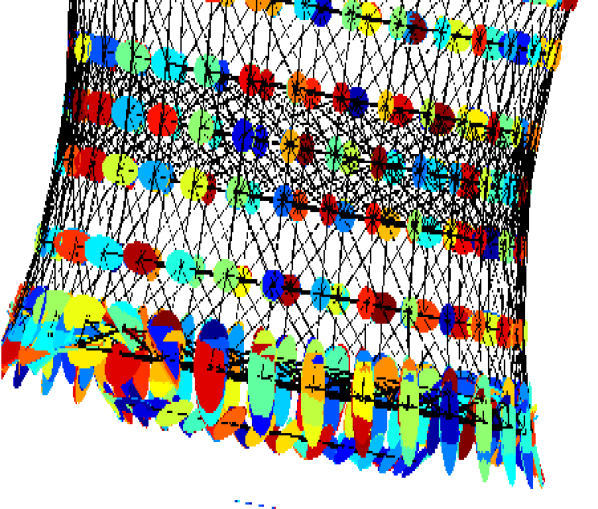
$h$ estimates, detail

Figure 2: Estimation of $h$ for a 2D hourglass-shaped manifold in 3D space. The embedding is obtained by Diffusion Maps. The ellipses attached to each point represent the embedding metric $h_{n}$ estimate for this embedding. At each data point $p\in\mathcal{P}$, $h_{n}(p)$ is a $3\times 3$ symmetric semi-positive definite matrix of rank 2. Near the “girth” of the hourglass, the ellipses are round, showing that the local geometry is recovered correctly. Near the top and bottom of the hourglass, the elongation of the ellipses indicates that distances are larger along the direction of elongation than the embedding suggests. For clarity, in the embedding displayed, the manifold was sampled regularly and sparsely. The black edges show the neigborhood graph $\mathcal{G}$ that was used. For all images in this figure, the color code has no particular meaning.

We constructed the next example to demonstrate how our method applies to the popular Sculpture Faces data set. This data set was introduced by Tenenbaum et al. (2000) along with Isomap as a prototypical example of how to recover a simple low dimensional manifold embedded in a high dimensional space. Specifically, the data set consists of $n=698$ $64\times 64$ gray images of faces. The faces are allowed to vary in three ways: the head can move up and down; the head can move right to left; and finally the light source can move right to left. With only three degrees of freedom, the faces define a three-dimensional manifold in the space of all $64\times 64$ gray images. In other words, we have a three-dimensional manifold $\mathcal{M}$ embedded in $[0,1]^{4096}$.

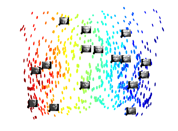
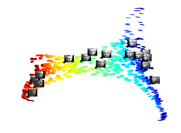
(a)	(b)
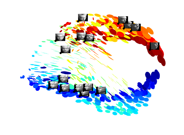
(c)

Figure 3: Two-dimensional visualization of the faces manifold, along with embedding. The color scheme corresponds to the left-right motion of the faces. The embeddings shown are: (a) Isomap, (b) LTSA, and Diffusion Maps ($\lambda=1$) (c).

As expected given its focus on preserving the geodesic distances, the Isomap seems to recover the simple rectangular geometry of the data set, as Figure 3 shows. LTSA, on the other hand, distorts the original data, particularly in the corners, where the Riemannian metric takes the form of thin ellipses. Diffusion Maps distorts the original geometry the most. The fact that the embedding for which we have theoretical guarantees of consistency causes the most distortion highlights, once more, that consistency provides no information about the level of distortion that may be present in the embedding geometry.

Our next example, Figure 4, shows an almost isometric reconstruction of a common example, the Swiss roll with a rectangular hole in the middle. This is a popular test data set because many algorithms have trouble dealing with its unusual topology. In this case, the LTSA recovers the geometry of the manifold up to an affine transformation. This is evident from the deformation of the embedding metric, which is parallel for all points in Figure 4 (b).

One would hope that such an affine transformation of the correct geometry would be easy to correct; not surprisingly, it is. In fact, we can do more than correct it: for any embedding, there is a simple transformation that turns the embedding into a local isometry. Obviously, in the case of an affine transformation, locally isometric implies globally isometric. We describe these transformations along with a few two-dimensional examples in the context of data visualization in the following section.

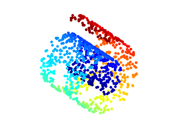
(a)	(b)

Figure 4: (a) Swissroll with a hole in ${\mathbb{R}}^{3}$. (b) LTSA embedding of the manifold in ${\mathbb{R}}^{2}$ along with metric.

6.2 Locally Isometric Visualization

Visualizing a manifold in a way that preserves the manifold geometry means obtaining an isometric embedding of the manifold in 2D or 3D. This is obviously not possible for all manifolds; in particular, only flat manifolds with intrinsic dimension below 3 can be “correctly visualized” according to this definition. This problem has been long known in cartography: a wide variety of cartographic projections of the Earth have been developed to map parts of the 2D sphere onto a plane, and each aims to preserve a different family of geometric quantities. For example, projections used for navigational, meteorological or topographic charts focus on maintaining angular relationships and accurate shapes over small areas; projections used for radio and seismic mapping focus on maintaining accurate distances from the center of the projection or along given lines; and projections used to compare the size of countries focus on maintaining accurate relative sizes (Snyder (1987)).

While the LearnMetric  algorithm is a general solution to preserving intrinsic geometry for all purposes involving calculations of geometric quantities, it cannot immediately give a general solution to the visualization problem described above.

However, it offers a natural way of producing locally isometric embeddings, and therefore locally correct visualizations for two- or three-dimensional manifolds. The procedure is based on the transformation of the points that will guarantee that the embedding is the identity matrix.

Given $(f_{n}(\mathcal{P}),h_{n}(\mathcal{P}))$ Metric Embedding of $\mathcal{P}$ 1. Select a point $p\in\mathcal{P}$ on the manifold 2. Transform coordinates $\tilde{f}_{n}(p^{\prime})\,\leftarrow\,h_{n}^{-1/2}(p)f_{n}(p^{\prime})$ for all $p^{\prime}\in\mathcal{P}$ Display $\mathcal{P}$ in coordinates $\tilde{f}_{n}$

As mentioned above, the transformation $\tilde{f}_{n}$ ensures that the embedding metric of $\tilde{f}_{n}$ is given by $\tilde{h}_{n}(p)=I_{s}$, i.e. the unit matrix at $p$. As $h$ varies smoothly on the manifold, $\tilde{h}_{n}$ should be close to $I_{s}$ at points near $p$, and therefore the embedding will be approximately isometric in a neighborhood of $p$.

Figures 5, 6 and 7 exemplify this procedure for the Swiss roll with a rectangular hole of Figure 4 embedded respectively by LTSA, Isomap and Diffusion Maps. In these figures, we use the Procrustes method (Goldberg and Ritov (2009)) to align the original neighborhood of the chosen point $p$ with the same neighborhood in an embedding. The Procrustes method minimizes the sum of squared distances between corresponding points between all possible rotations, translations and isotropic scalings. The residual sum of squared distances is what we call the Procrustes dissimilarity. Its value is close to zero when the embedding is locally isometric around $p$.

$\bullet$ original	$\bullet$ embedding
$\bullet$	$\bullet$

Figure 5: Locally isometric visualization for the Swiss roll with a rectangular hole, embedded in $d=2$ dimensions by LTSA. Top left: LTSA embedding with selected point $p$ (red) and its neighbors (blue). Top right: locally isometric embedding. Middle left: Neighborhood of $p$ for the LTSA embedding. Middle right: Neighborhood of $p$ for the locally isometric embedding. Bottom left: Procrustes between the neighborhood of $p$ for the LTSA embedding and the original manifold projected on $T_{p}\mathcal{M}$; dissimilarity measure: $D=0.30$. Bottom right: Procrustes between the locally isometric embedding and the original manifold; dissimilarity measure: $D=0.02$.

$\bullet$ original	$\bullet$ embedding

Figure 6: Locally isometric visualization for the Swiss roll with a rectangular hole, embedded in $d=2$ dimensions by Isomap. Top left: Isomap embedding with selected point $p$ (red), and its neighbors (blue). Top right: locally isometric embedding. Middle left: Neighborhood of $p$ for the Isomap embedding. Middle right: Neighborhood of $p$ for the locally isometric embedding. Bottow left: Procrustes between the neighborhood of the $p$ for the Isomap embedding and the original manifold projected on $T_{p}\mathcal{M}$; dissimilarity measure: $D=0.21$. Bottom right: Procrustes between the locally isometric embedding and the original manifold; dissimilarity measure: $D=0.06$.

$\bullet$ original	$\bullet$ embedding

Figure 7: Locally isometric visualization for the Swiss roll with a rectangular hole, embedded in $d=2$ dimensions by Diffusion Maps ($\lambda=1$). Top left: DM embedding with selected point $p$ (red), and its neighbors (blue). Top right: locally isometric embedding. Middle left: Neighborhood of $p$ for the DM embedding. Middle right: Neighborhood of $p$ for the locally isometric embedding. Bottow left: Procrustes between the neighborhood of the $p$ for the DM embedding and the original manifold projected on $T_{p}\mathcal{M}$; dissimilarity measure: $D=0.10$. Bottom right: Procrustes between the locally isometric embedding and the original manifold; dissimilarity measure: $D=0.07$.

6.3 Estimation of Geodesic Distances

The geodesic distance $d_{\mathcal{M}}(p,p^{\prime})$ between two points $p,p^{\prime}\in\mathcal{M}$ is defined as the length of the shortest curve from $p$ to $p^{\prime}$ along manifold $\mathcal{M}$, which in our example is a half sphere of radius 1. The geodesic distance $d$ being an intrinsic quantity, it should evidently not change with the parametrization.

We performed the following numerical experiment. First, we sampled $n=1000$ points uniformly on a half sphere. Second, we selected two reference points $p,p^{\prime}$ on the half sphere so that their geodesic distance would be $\pi/2$. We then proceeded to run three manifold learning algorithms on $\mathcal{P}$, obtaining the Isomap, LTSA and DM embeddings. All the embeddings used the same 10-nearest neighborhood graph $G$.

For each embedding, and for the original data, we calculated the naive distance $||f_{n}(p)-f_{n}(p^{\prime})||$. In the case of the original data, this represents the straight line that connects $p$ and $p^{\prime}$ and crosses through the ambient space. For Isomap, $||f_{n}(p)-f_{n}(p^{\prime})||$ should be the best estimator of $d_{\mathcal{M}}(p,p^{\prime})$, since Isomap embeds the data by preserving geodesic distances using MDS. As for LTSA and DM, this estimator has no particular meaning, since these algorithms are derived from eigenvectors, which are defined up to a scale factor.

We also considered the graph distance, by which we mean the shortest path between the points in $G$, where the distance is given by $||f_{n}(q_{i})-f_{n}(q_{i-1}^{\prime})||$:

$${d}_{\mathcal{G}}(p,p^{\prime})\;=\;\underset{\text{paths}}{\min}\{\sum_{i=1}^{l}||f_{n}(q_{i})-f_{n}(q_{i-1})||,\,(q_{0}=p,\,q_{1},\,q_{2},\ldots\,q_{l}=p^{\prime})\,\mbox{\rm path in}\;\mathcal{G}\}.$$ (22)

Note that although we used the same graph $\mathcal{G}$ to generate all the embeddings, the shortest path between points may be different in each embedding since the distances between nodes will generally not be preserved.

The graph distance $d_{\mathcal{G}}$ is a good approximation for the geodesic distance $d$ in the original data and in any isometric embedding, as it will closely follow the actual manifold rather then cross in the ambient space.

Finally, we computed the discrete minimizing geodesic as:

$$\hat{d}_{\mathcal{M}}(p,p^{\prime})\;=\;\underset{\text{paths}}{\min}\{\sum_{i=1}^{l}\mathcal{H}(q_{i},q_{i-1}),\,(q_{0}=p,\,q_{1},\,q_{2},\ldots\,q_{l}=p^{\prime})\,\mbox{\rm path in}\;\mathcal{G}\}$$ (23)

where

$$\mathcal{H}(q_{i},q_{i-1}) = \frac{1}{2}\sqrt{(f_{n}(q_{i})-f_{n}(q_{i-1}))^{t}h_{n}(q_{i})(f_{n}(q_{i})-f_{n}(q_{i-1}))}$$ (24)

$$+\frac{1}{2}\sqrt{(f_{n}(q_{i})-f_{n}(q_{i-1}))^{t}h_{n}(q_{i-1})(f_{n}(q_{i})-f_{n}(q_{i-1}))}$$

is the discrete analog of the path-length formula (3) for the Voronoi tesselation of the space. By Voronoi tesselation, we mean the partition of the space into sets based on $\mathcal{P}$ such that each set consists of all points closest to a single point in $\mathcal{P}$ than any other. Figure 8 shows the manifolds that we used in our experiments, and Table 1 displays the estimated distances.

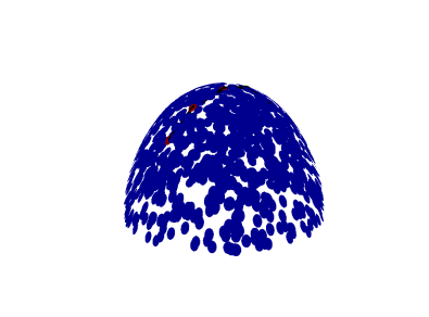
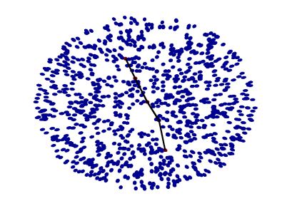
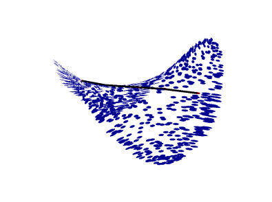
(a)	(b)	(c)

Figure 8: Manifold and embeddings (black) used to compute the geodesic distance. Points that were part of the geodesic, including endpoints, are shown in red, while the path is shown in black. The LTSA embedding is not shown here: it is very similar to the Isomap. (a) Original manifold (b) Diffusion Maps (c) Isomap.

		Shortest
Embedding	$||f_{n}(p)-f_{n}(p^{\prime})||$	Path $d_{\mathcal{G}}$	Metric $\hat{d}$	$\hat{d}$ Relative Error
Original data	1.412	1.565 $\pm$ 0.003	1.582 $\pm$ 0.006	0.689 %
Isomap $s=2$	1.738 $\pm$ 0.027	1.646 $\pm$ 0.016	1.646 $\pm$ 0.029	4.755%
LTSA $s=2$	0.054 $\pm$ 0.001	0.051 $\pm$ 0.0001	1.658 $\pm$ 0.028	5.524%
DM $s=3$	0.204 $\pm$ 0.070	0.102 $\pm$ 0.001	1.576 $\pm$ 0.012	0.728%

Table 1: Distance estimates (mean and standard deviation) for a sample size of $n=2000$ points was used for all embeddings while the standard deviations were estimated by repeating the experiment 5 times. The relative errors in the last column were computed with respect to the true distance $d=\pi/2\simeq$1.5708.

As expected, for the original data, $||p-p^{\prime}||$ necessarily underestimates $d_{\mathcal{M}}$, while $d_{\mathcal{G}}$ is a very good approximation of $d_{\mathcal{M}}$, since it follows the manifold more closely. Meanwhile, the opposite is true for Isomap. The naive distance $||f_{n}(p)-f_{n}(p^{\prime})||$ is close to the geodesic by construction, while $d_{\mathcal{G}}$ overestimates $d_{\mathcal{M}}$ since $d_{\mathcal{G}}\geq||f_{n}(p)-f_{n}(p^{\prime})||$ by the triangle inequality. Not surprisingly, for LTSA and Diffusion Maps, the estimates $||f_{n}(p)-f_{n}(p^{\prime})||$ and $d_{\mathcal{G}}$ have no direct correspondence with the distances of the original data since these algorithms make no attempt at preserving absolute distances.

However, the estimates $\hat{d}$ are quite similar for all embedding algorithms, and they provide a good approximation for the true geodesic distance. It is interesting to note that $\hat{d}$ is the best estimate of the true geodesic distance even for the Isomap, whose focus is specifically to preserve geodesic distances. In fact, the only estimate that is better than $\hat{d}$ for any embedding is the graph distance on the original manifold.

6.4 Volume Estimation

The last set of our experiments demonstrates the use of the Riemannian metric in estimating two-dimensional volumes: areas. We used an experimental procedure similar to the case of geodesic distances, in that we created a two-dimensional manifold, and selected a set $W$ on it. We then estimated the area of this set by generating a sample from the manifold, embedding the sample, and computing the area in the embedding space using a discrete form of (4).

One extra step is required when computing areas that was optional when computing distances: we need to construct coordinate chart(s) to represent the area of interest. Indeed, to make sense of the Euclidean volume element $dx^{1}\ldots dx^{d}$, we need to work in ${\mathbb{R}}^{d}$. Specifically, we resort to the idea expressed at the end of Section 4.2, which is to project the embedding on its tangent at the point $p$ around which we wish to compute $dx^{1}\ldots dx^{d}$. This tangent plane $T_{f(p)}f(\mathcal{M})$ is easily identified from the SVD of $h_{n}(p)$ and its singular vectors with non-zero singular values. It is then straightforward to use the projection $\Pi$ of an open neighborhood $f(U)$ of $f(p)$ onto $T_{f(p)}f(\mathcal{M})$ to define the coordinate chart $(U,x=\Pi\circ f)$ around $p$. Since this is a new chart, we need to recompute the embedding metric ${h_{n}}$ for it.

By performing a tessellation of $(U,x=\Pi\circ f)$ (we use the Voronoi tesselation for simplicity), we are now in position to compute $\triangle x^{1}\ldots\triangle x^{d}$ around $p$ and multiply it by $\sqrt{\det{({h_{n}})}}$ to obtain $\triangle\text{Vol}\simeq d\text{Vol}$. Summing over all points of the desired set gives the appropriate estimator:

$$\hat{\text{Vol}}(W)=\sum_{p\in W}\sqrt{\det{({h_{n}(p)})}}\triangle x^{1}(p)\ldots\triangle x^{d}(p)\,.$$ (25)

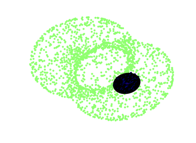
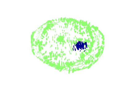
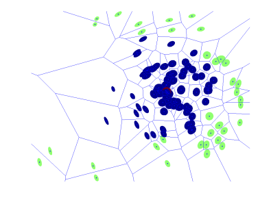
(a)	(b)	(c)

Figure 9: (a) Manifold along with $W$, the computed area in black. (b) Diffusion Maps ($\lambda=1$) embedding with embedding metric $h$. (c) A locally isometric coordinate chart constructed from the Diffusion Maps along with the Voronoi tessellation. For Figures (b) and (c), the point at the center of $W$ is in red, the other points in $W$ are in blue and the points not in $W$ are in green.The sample size is $n=1000$.

Embedding	Naive Area of $W$	$\hat{\text{Vol}}(W)$	$\hat{\text{Vol}}(W)$ Relative Error
Original data	2.63 $\pm$ 0.10†	2.70 $\pm$ 0.10	2.90%
Isomap	6.53 $\pm$ 0.34†	2.74 $\pm$ 0.12	3.80%
LTSA	8.52e-4 $\pm$ 2.49e-4	2.70 $\pm$ 0.10	2.90 %
DM	6.70e-4 $\pm$ 0.464e-04†	2.62 $\pm$ 0.13	4.35 %

Table 2: Estimates of the volume of $W$ on the hourglass depicted in Figure 9, based on 1000 sampled points. The experiment was repeated five times to obtain a variance for the estimators. ^†The naive area/volume estimator is obtained by projecting the manifold or embedding on $T_{p}\mathcal{M}$ and $T_{f(p)}f(\mathcal{M})$, respectively. This requires manually specifying the correct tangent planes, except for LTSA, which already estimates $T_{f(p)}f(\mathcal{M})$. Similarly to LTSA, $\hat{\text{Vol}}(W)$ is constructed so that the embedding is automatically projected on $T_{f(p)}f(\mathcal{M})$. Here, the true area is $2.658$

Table 2 reports the results of our comparison of the performance of $\hat{\text{Vol}}(W)$, described in 25 , and a “naive” volume estimator that computes the area on the Voronoi tessellation once the manifold is projected onto the tangent plane. We find that $\hat{\text{Vol}}(W)$ performs better for all embeddings, as well as for the original data. The latter is explained by the fact that when we project the set $W$ onto the tangent plane $T_{f(p)}f(\mathcal{M})$, we induce a fair amount of distortion, and the naive estimator has no way of correcting for it.

The relative error for LTSA is similar to that for the original data and larger than for the other methods. One possible reason for this is the error in estimating the tangent plane ${\cal T}_{p}\mathcal{M}$, which, in the case of these two methods, is done by local PCA.

7 Conclusion and Discussion

In this article, we have described a new method for preserving the important geometrical information in a data manifold embedded using any embedding algorithm. We showed that the Laplace-Beltrami operator can be used to augment any reasonable embedding so as to allow for the correct computation of geometric values of interest in the embedding’s own coordinates.

Specifically, we showed that the Laplace-Beltrami operator allows us to recover a Riemannian manifold $(\mathcal{M},g)$ from the data and express the Riemannian metric $g$ in any desired coordinate system. We first described how to obtain the Riemannian metric from the mathematical, algorithmic and statistical points of view. Then, we proceeded to describe how, for any mapping produced by an existing manifold learning algorithm, we can estimate the Riemannian metric $g$ in the new data coordinates, which makes the geometrical quantities like distances and angles of the mapped data (approximately) equal to their original values, in the raw data. We conducted several experiments to demonstrate the usefulness of our method.

Our work departs from the standard manifold learning paradigm. While existing manifold learning algorithms, when faced with the impossibility of mapping curved manifolds to Euclidean space, choose to focus on distances, angles, or specific properties of local neighborhoods and thereby settle for trade-offs, our method allows for dimensionality reduction without sacrificing any of these data properties. Of course, this entails recovering and storing more information than the coordinates alone. The information stored under the Metric Learning algorithm is of order $s^{2}$ per point, while the coordinates only require $s$ values per point.

Our method essentially frees users to select their preferred embedding algorithm based on considerations unrelated to the geometric recovery; the metric learning algorithm then obtains the Riemannian metric corresponding to these coordinates through the Laplace-Beltrami operator. Once these are obtained, the distances, angles, and other geometric quantities can be estimated in the embedded manifold by standard manifold calculus. These quantities will preserve their values from the original data and are thus embedding-invariant in the limit of $n\rightarrow\infty$.

Of course, not everyone agrees that the original geometry is interesting in and of itself; sometimes, it should be discarded in favor of a new geometry that better highlights the features of the data that are important for a given task. For example, clustering algorithms stress the importance of the dissimilarity (distance) between different clusters regardless of what the original geometry dictates. This is in fact one of the arguments advanced by Nadler et al. (2006) in support of spectral clustering which pulls points towards regions of high density.

Even in situations where the new geometry is considered more important, however, understanding the relationship between the original and the new geometry using Metric Learning - and, in particular, the pullback metric Lee (2003) - could be of value and offer further insight. Indeed, while we explained in Section 6 how the embedding metric $h$ can be used to infer how the original geometry was affected by the map $f$, we note at this juncture that the pullback metric, i.e. the geometry of $(f(\mathcal{M}),\delta_{s})$ pulled back to $\mathcal{M}$ by the map $f$, can offer interesting insight into the effect of the transformation/embedding. In fact, this idea has already been considered by Burges (1999) in the case of kernel methods where one can compute the pullback metric directly from the definition of the kernel used. In the framework of Metric Learning, this can be extended to any transformation of the data that defines an embedding.

References

- Behmardi and Raich (2010) B. Behmardi and R. Raich. Isometric correction for manifold learning. In AAAI Symposium on Manifold Learning, 2010.
- Belkin and Niyogi (2002) M. Belkin and P. Niyogi. Laplacian eigenmaps for dimensionality reduction and data representation. Neural Computation, 15:1373–1396, 2002.
- Belkin and Niyogi (2007) M. Belkin and P. Niyogi. Convergence of laplacians eigenmaps. In Advances in Neural Information Processing Systems (NIPS), 2007.
- Belkin et al. (2009) M. Belkin, J. Sun, and Y. Wang. Constructing laplace operator from point clouds in rd. In ACM-SIAM Symposium on Discrete Algorithms, pages 1031–1040, 2009.
- Ben-Israel and Greville (2003) A. Ben-Israel and T. N. E. Greville. Generalized inverses: Theory and applications. Springer, New York, 2003.
- Bernstein et al. (2000) M. Bernstein, V. deSilva, J. C. Langford, and J. Tennenbaum. Graph approximations to geodesics on embedded manifolds, 2000. URL http://web.mit.edu/cocosci/isomap/BdSLT.pdf.
- Borg and Groenen (2005) I. Borg and P. Groenen. Modern Multidimensional Scaling: Theory and Applications. Springer-Verlag, 2nd edition, 2005.
- Burges (1999) C. J. C. Burges. Geometry and invariance in kernel based methods. Advances in Kernel Methods - Support Vector Learning, 1999.
- Coifman and Lafon (2006) R. R. Coifman and S. Lafon. Diffusion maps. Applied and Computational Harmonic Analysis, 21(1):6–30, 2006.
- Dreisigmeyer and Kirby (2007, retrieved June 2010) D. W. Dreisigmeyer and M. Kirby. A pseudo-isometric embedding algorithm, 2007, retrieved June 2010. URL http://www.math.colostate.edu/~thompson/whit_embed.pdf.
- Giné and Koltchinskii (2006) E. Giné and V. Koltchinskii. Empirical Graph Laplacian Approximation of Laplace-Beltrami Operators: Large Sample results. High Dimensional Probability, pages 238–259, 2006.
- Goldberg and Ritov (2009) Y. Goldberg and Y. Ritov. Local procrustes for manifold embedding: a measure of embedding quality and embedding algorithms. Machine Learning, 77(1):1–25, 2009.
- Goldberg et al. (2008) Y. Goldberg, A. Zakai, D. Kushnir, and Y. Ritov. Manifold Learning: The Price of Normalization. Journal of Machine Learning Research, 9:1909–1939, 2008.
- Hein et al. (2007) M. Hein, J.-Y. Audibert, and U. von Luxburg. Graph Laplacians and their Convergence on Random Neighborhood Graphs. Journal of Machine Learning Research, 8:1325–1368, 2007.
- Lee (1997) J. M. Lee. Riemannian Manifolds: An Introduction to Curvature. Springer, New York, 1997.
- Lee (2003) J. M. Lee. Introduction to Smooth Manifolds. Springer, New York, 2003.
- Nadler et al. (2006) B. Nadler, S. Lafon, and R. R. Coifman. Diffusion maps, spectral clustering and eigenfunctions of fokker-planck operators. In Advances in Neural Information Processing Systems (NIPS), 2006.
- Nash (1956) J. Nash. The imbedding problem for Riemannian manifolds. Annals of Mathematics, 63:20–63, 1956.
- Ram et al. (2009) P. Ram, D. Lee, W. March, and A. G. Gray. Linear-time algorithms for pairwise statistical problems. In Advances in Neural Information Processing Systems (NIPS), 2009.
- Rosenberg (1997) S. Rosenberg. The Laplacian on a Riemannian Manifold. Cambridge University Press, 1997.
- Saul and Roweis (2003) L. Saul and S. Roweis. Think globally, fit locally: unsupervised learning of low dimensional manifold. Journal of Machine Learning Research, 4:119–155, 2003.
- Snyder (1987) J. P. Snyder. Map Projections: A Working Manual. United States Government Printing, 1987.
- Tenenbaum et al. (2000) J. Tenenbaum, V. deSilva, and J. C. Langford. A global geometric framework for nonlinear dimensionality reduction. Science, 290:2319–2323, 2000.
- Ting et al. (2010) D. Ting, L Huang, and M. I. Jordan. An analysis of the convergence of graph laplacians. In International Conference on Machine Learning, pages 1079–1086, 2010.
- von Luxburg et al. (2008) U. von Luxburg, M. Belkin, and O. Bousquet. Consistency of spectral clustering. Annals of Statistics, 36(2):555–585, 2008.
- Weinberger and Saul (2006) K.Q. Weinberger and L.K. Saul. Unsupervised learning of image manifolds by semidefinite programming. International Journal of Computer Vision, 70:77–90, 2006.
- Wittman (2005, retrieved 2010) T. Wittman. Manifold learning matlab demo, 2005, retrieved 2010. URL http://www.math.umn.edu/~wittman/mani/.
- Zha and Zhang (2003) H. Zha and Z. Zhang. Isometric embedding and continuum isomap. In International Conference on Machine Learning, pages 864–871, 2003.
- Zhang and Zha (2004) Z. Zhang and H. Zha. Principal manifolds and nonlinear dimensionality reduction via tangent space alignment. Society for Industrial and Applied Mathematics Journal of Scientific Computing, 26(1):313–338, 2004.
- Zhou and Belkin (2011) X. Zhou and M. Belkin. Semi-supervised learning by higher order regularization. In The 14th International Conference on Artificial Intelligence and Statistics, 2011.