Abstract

We study a probabilistic numerical method for the solution of both boundary and initial value problems that returns a joint Gaussian process posterior over the solution. Such methods have concrete value in the statistics on Riemannian manifolds, where non-analytic ordinary differential equations are involved in virtually all computations. The probabilistic formulation permits marginalising the uncertainty of the numerical solution such that statistics are less sensitive to inaccuracies. This leads to new Riemannian algorithms for mean value computations and principal geodesic analysis. Marginalisation also means results can be less precise than point estimates, enabling a noticeable speed-up over the state of the art. Our approach is an argument for a wider point that uncertainty caused by numerical calculations should be tracked throughout the pipeline of machine learning algorithms.

1 Introduction

Systems of ordinary differential equations (ODEs), defined here as equations of the form

$$c^{(n)}(t)=f(c(t),c^{\prime}(t),\dots,c^{(n-1)}(t),t)$$ (1)

with $c:\mathbb{R}\operatorname*{\rightarrowtriangle}\mathbb{R}^{D}$ and $f:\mathbb{R}^{nD}\times\mathbb{R}\operatorname*{\rightarrowtriangle}\mathbb{R}^{D}$ are essential tools of numerical mathematics. In machine learning and statistics, they play a role in the prediction of future states in dynamical settings, but another area where they have a particularly central role are statistical computations on Riemannian manifolds. On such manifolds, the distance between two points is defined as the length of the shortest path connecting them, and calculating this path requires solving ordinary differential equations. Distances are elementary, so virtually all computations in Riemannian statistics involve numerical ODE solvers (Sec. 2). Just calculating the mean of a dataset of $P$ points, trivial in Euclidean space, requires optimisation of $P$ geodesics, thus the repeated solution of $P$ ODEs. Errors introduced by this heavy use of numerical machinery are structured and biased, but hard to quantify, mostly because numerical solvers do not return sufficiently structured error estimates.

The problem of solving ordinary differential equations is very well studied (Hairer et al. (1987, §1) give a historical overview), and modern ODE solvers are highly evolved. But at their core they are still based on the seminal work of Runge (1895) and Kutta (1901), a carefully designed process of iterative extrapolation. In fact, ODE solvers, like other numerical methods, can be interpreted as inference algorithms (Diaconis, 1988; O’Hagan, 1992), in that they estimate an intractable quantity (the ODE’s solution) given “observations” of an accessible quantity (values of $f$). Like all estimators, these methods are subject to an error between estimate and truth. Modern solvers can estimate this error (Hairer et al., 1987, §II.3 & §II.4), but generally only as a numerical bound at the end of each local step, not in a functional form over the space of solutions. In this paper we study and extend an idea originally proposed by John Skilling (1991) to construct (Sec. 3) a class of probabilistic solvers for both boundary value problems (BVPs) and initial value problems (IVPs). Our version of Skilling’s algorithm returns nonparametric posterior probability measures over the space of solutions of the ODE. This kind of structured uncertainty improves Riemannian statistics, where the solution of the ODE is a latent “nuisance” variable. As elsewhere, it is beneficial to replace point estimates over such variables with probability distributions and marginalise over them (Sec. 4). A second, remarkable result is that, although the probabilistic solver presented here provides additional functionality, when applied to concrete problems in Riemannian statistics, it can actually be faster than standard boundary value problem solvers (as implemented in Matlab). One reason is that the answers returned by the probabilistic solver can be less precise, because small errors are smoothed out when marginalised over the posterior uncertainty. As the cost of Riemannian statistics is dominated by that of solving ODEs, time saved by being “explicitly sloppy” in the probabilistic sense is of great value. Sec. 5 offers some empirical evaluations. A Matlab implementation of the solver is published alongside this manuscript.

The focus of this text is on the concrete case of Riemannian statistics and ODEs. But we believe it to be a good example for the value of probabilistic numerical methods to machine learning and statistics more generally. Treating numerical algorithms as black boxes ignores their role as error sources and can cause unnecessary computational complexity. Our results show that algorithms designed with probabilistic calculations in mind can offer qualitative and quantitative benefits. In particular, they can propagate uncertainty through a numerical computation, providing a joint approximate distribution between input and output of the computation.

2 Riemannian Statistics

Statistics on Riemannian manifolds is becoming increasingly acknowledged as it allows for statistics in constrained spaces, and in spaces with a smoothly changing metric. Examples include analysis of shape (Freifeld and Black, 2012; Fletcher et al., 2004), human poses (Hauberg et al., 2012b) and image features (Porikli et al., 2006). Here we focus on Riemannian statistics in metric learning, where a smoothly changing metric locally adapts to the data (Hauberg et al., 2012a).

Let $M(x)\in\mathbb{R}^{D\times D}$ denote a positive definite, smoothly changing, metric tensor function at $x\in\mathbb{R}^{D}$. It locally defines a norm $\|y\|^{2}_{M(x)}=y^{\intercal}M(x)y$. This norm in turn defines (Berger, 2007) the length of a curve $c:[0,1]\operatorname*{\rightarrowtriangle}\mathbb{R}^{D}$ as $\mathrm{Length}(c):=\int_{0}^{1}\|c^{\prime}(t)\|_{M(c(t))}\mathrm{d}t$. For two points $a$, $b$, the shortest connecting curve, $c=\operatorname*{arg\>min}_{\hat{c}}\mathrm{Length}(\hat{c})$ is known as a geodesic, and defines the distance between $a$ and $b$ on the manifold. Using the Euler-Lagrange equation, it can be shown (Hauberg et al., 2012a) that geodesics must satisfy the system of homogenous second-order boundary value problems

$$c^{\prime\prime}(t) =-\frac{1}{2}M^{-1}(c(t))\left[\frac{\partial\vv{M}(c(t))}{\partial c(t)}\right]^{\intercal}[c^{\prime}(t)\otimes c^{\prime}(t)$$

$$=:f(c(t),c^{\prime}(t)),\text{ with }c(0)=a,c(1)=b.$$ (2)

where the notation $\vv{M}$ indicates the vectorization operation returning a vector $\in\mathbb{R}^{D^{2}}$, formed by stacking the elements of the $D\times D$ matrix $M$ row by row, and $\otimes$ is the Kronecker product, which is associated with the vectorization operation (van Loan, 2000). The short-hand $f(c(t),c^{\prime}(t))$ is used throughout the paper. For simple manifolds this BVP can be solved analytically, but most models of interest require numerical solutions.

The geodesic starting at $a$ with initial direction $v$ is given by the initial value problem

$$c^{\prime\prime}(t)=f(c(t),c^{\prime}(t)),\quad c(0)=a\quad\mathrm{and}\quad c^{\prime}(0)=v.$$ (3)

By the Picard–Lindelöf theorem (Tenenbaum and Pollard, 1963), this curve exists and is locally unique. As $v$ is the derivative of a curve on the manifold at $a$, it belongs to the tangent space of the manifold at $a$. Eq. (3) implies that geodesics can be fully described by their tangent $v$ at $c(0)$. This observation is a corner-stone of statistical operations on Riemannian manifolds, which typically start with a point $\mu$ (often the mean), compute geodesics from there to all data points, and then perform Euclidean statistics on the tangents $v_{1:P}$ at $\mu$. This implicitly gives statistics of the geodesics.

These concepts are formalised by the exponential and logarithm maps, connecting the tangent space and the manifold. The exponential map $\mathrm{Exp}_{a}(v)$ returns the end-point of the geodesic $c$ satisfying Eq. (3) such that $\mathrm{Length}(c)=\|v\|$. The logarithm map $\mathrm{Log}_{a}(b)$ is the inverse of the exponential map. It returns the initial direction of the geodesic from $a$ to $b$, normalised to the length of the geodesic, i.e.

$$\mathrm{Log}_{a}(b)=\frac{c^{\prime}(0)}{\|c^{\prime}(0)\|}\mathrm{Length}(c).$$ (4)

The following paragraphs give examples for how this theory is used in statistics, and how the use of numerical solvers in these problems affect the results and their utility, thus motivating the use of a probabilistic solver.

Means on Manifolds

The most basic statistic of interest is the mean, which is defined as the minimiser of the sum of squared distances on the manifold. A global minimiser is called the Frechét mean, while a local minimiser is called a Karcher mean (Pennec, 1999). In general, closed-form solutions do not exist and gradient descent is applied; the update rule of $\mu_{k}$ with learning rate $\alpha$ is (Pennec, 1999)

$$\mu_{k+1}=\mathrm{Exp}_{\mu_{k}}\left(\alpha\frac{1}{P}\sum_{i=1}^{P}\mathrm{Log}_{\mu_{k}}(x_{i})\right).$$ (5)

One practical issue is that, in each iteration, the exponential and logarithm maps need to be computed numerically. Each evaluation of Eq. (5) requires the solution of $P$ BVPs and one IVP. Practitioners thus perform only a few iterations rather than run gradient descent to convergence. Intuitively, it is clear that these initial steps of gradient descent do not require high numerical precision. The solver should only control their error sufficiently to find a rough direction of descent.

Principal Geodesic Analysis

A generalisation of principal component analysis (PCA) to Riemannian manifolds is principal geodesic analysis (PGA) (Fletcher et al., 2004). It performs ordinary PCA in the tangent space at the mean, i.e. the principal directions are found as the eigenvectors of $\mathrm{Log}_{\mu}(x_{1:P})$, where $\mu$ is the mean as computed by Eq. (5). The principal direction $v$ is then mapped back to the manifold to form principal geodesics via the exponential map, i.e. $\gamma(t)=\mathrm{Exp}_{\mu}(tv)$.

Again, this involves solving for $P$ geodesics: one from each $x_{i}$ to the mean. As the statistics are performed on the (notoriously unstable) derivatives of the numerical solutions, here, high-accuracy solvers are required. These computational demands only allow for low-sample applications of PGA.

Applications in Metric Learning

The original appeal of Riemannian statistics is that many types of data naturally live on known Riemannian manifolds (Freifeld and Black, 2012; Fletcher et al., 2004; Porikli et al., 2006), for example certain Lie groups. But a recent generalisation is to estimate a smoothly varying metric tensor from the data, using metric learning, and perform Riemannian statistics on the manifold implied by the smooth metric (Hauberg et al., 2012a). The idea is to regress a smoothly changing metric tensor from learned metrics $M_{1:R}$ as

$$M(x) =\sum_{r=1}^{R}\frac{\tilde{w}_{r}(x)}{\sum_{j=1}^{R}\tilde{w}_{j}(x)}M_{r},\qquad\mathrm{where}$$ (6)

$$\tilde{w}_{r}(x) =\exp\left(-\frac{\rho}{2}(x-\mu_{r})^{\intercal}M_{r}(x-\mu_{r})\right).$$ (7)

As above, geodesics on this manifold require numeric solutions; hence this approach is currently only applicable to fairly small problems. The point estimates returned by numerical solvers, and their difficult to control computational cost, are both a conceptual and computational roadblock for the practical use of Riemannian statistics. A method returning explicit probabilistic error estimates, at low cost, is needed.

3 Solving ODEs with Gaussian process priors

Writing in 1991, John Skilling proposed treating initial value problems as a recursive Gaussian regression problem: Given a Gaussian estimate for the solution of the ODE, one can evaluate a linearization of $f$, thus construct a Gaussian uncertain evaluation of the derivative of $c$, and use it to update the belief on $c$. The derivations below start with a compact introduction to this idea in a contemporary notation using Gaussian process priors, which is sufficiently general to be applicable to both boundary and initial values. Extending Skilling’s method, we introduce a way to iteratively refine the estimates of the method similar to implicit Runge-Kutta methods, and a method to infer the hyperparameters of the algorithm.

The upshot of these derivations is a method returning a nonparametric posterior over the solution of both boundary and initial value problems. Besides this more expressive posterior uncertainty, another functional improvement over contemporary solvers is that these kind of algorithms allow for Gaussian uncertainty on the boundary or initial values, an essential building block of probabilistic computations.

In parallel work, Chkrebtii et al. (2013) have studied several theoretical aspects of Skilling’s method thoroughly. Among other things, they provide a proof of consistency of the probabilistic estimator and argue for the uniqueness of Gaussian priors on ODE and PDE solutions. Here, we focus on the use of such probabilistic numerical methods within a larger (statistical) computational pipeline, to demonstrate the strengths of this approach, argue for its use, and highlight open research questions. We also offer a minor theoretical observation in Section 3.5, to highlight a connection between Skilling’s approach and the classic Runge-Kutta framework that has previously been overlooked.

Conceptually, the algorithm derived in the following applies to the general case of Eq. (42). For concreteness and simplicity of notation, though, we focus on the case of a second-order ODE. All experiments will be performed in the Riemannian context, where the object to be inferred is the geodesic curve $c:t\in\mathbb{R}\mapsto c(t)\in\mathbb{R}^{D}$ consistent with Eqs. (43) or (3): Distance calculations between two points are boundary value problems of the form $c(0)=a$, $c(1)=b$. Shifts of variables along geodesics are initial value problems of the form $c(0)=a$, $c^{\prime}(0)=v$ where $v$ is the length of the geodesic. The probabilistically uncertain versions of these are

$$p(c(0),c(1)) =\mathcal{N}(c(0);a,\Delta_{a})\mathcal{N}(c(1);b,\Delta_{b}),\text{ or}$$ (8)

$$p(c(0),c^{\prime}(0)) =\mathcal{N}(c(0);a,\Delta_{a})\mathcal{N}(c^{\prime}(0);v,\Delta_{v}).$$ (9)

with positive semidefinite covariance matrices $\Delta_{a},\Delta_{b},\Delta_{v}\in\mathbb{R}^{D\times D}$.

3.1 Prior

We assign a joint Gaussian process prior over the elements of the geodesic, with a covariance function factorizing between its input and output dependence ($c_{i}(t)$ is the $i$-th element of $c(t)\in\mathbb{R}^{D}$):

$$p(c(t))=\mathcal{GP}(c;\mu_{c},V\otimes k),\qquad\text{that is,}$$ (10)

$$\operatorname{cov}(c_{i}(t_{1}),c_{j}(t_{2}))=V_{ij}k(t_{1},t_{2}),$$

with a positive semidefinite matrix $V$ – the covariance between output dimensions, and a positive semidefinite kernel $k:\mathbb{R}\times\mathbb{R}\operatorname*{\rightarrowtriangle}\mathbb{R}$ defining the covariance between scalar locations along the curve. The geodesic problem only involves values $t\in[0,1]$, but this restriction is not necessary in general. The mean functions $\mu_{c}:\mathbb{R}\operatorname*{\rightarrowtriangle}\mathbb{R}^{D}$ have only minor effects on the algorithm. For BVPs and IVPs, we choose linear functions $\mu(t)=a+(b-a)t$ and $\mu(t)=a+vt$, respectively. There is a wide space of covariance functions available for Gaussian process regression (Rasmussen and Williams, 2006, §4). In principle, every smooth covariance function can be used for the following derivations (more precisely, see Eq. (46) below). For our implementation we use the popular square-exponential (aka. radial basis function, Gaussian) kernel $k(t_{1},t_{2})=\exp\left[-(t_{1}-t_{2})^{2}/(2\lambda^{2})\right]$. This amounts to the prior assumption that geodesics are smooth curves varying on a length scale of $\lambda$ along $t$, with output covariance $V$. Sec. 3.4 below explains how to choose these hyperparameters.

Gaussian processes are closed under linear transformations. For any linear operator $A$, if $p(x)=\mathcal{GP}(x;\mu,k)$ then $p(Ax)=\mathcal{GP}(Ax;A\mu,AkA^{\intercal})$. In particular, a Gaussian process prior on the geodesics $c$ thus also implies a Gaussian process belief over any derivative $\partial^{n}c(t)/\partial t^{n}$ (see Rasmussen and Williams (2006, §9.4)), with mean function $\partial^{n}\mu(t)/\partial t^{n}$ and covariance function

$$\operatorname{cov}\left(\frac{\partial^{n}c_{i}(t_{1})}{\partial t_{1}^{n}},\frac{\partial^{n}c_{j}(t_{2})}{\partial t^{n}_{2}}\right)=V_{ij}\frac{\partial^{2n}k(t_{1},t_{2})}{\partial t_{1}^{n}\partial t_{2}^{n}},$$ (11)

provided the necessary derivatives of $k$ exist, as they do for the square-exponential kernel $\forall n\in\mathbb{N}$. Explicit algebraic forms for the square-exponential kernel’s case can be found in the supplements.

The boundary or initial values $a,b$ or $a,v$, can be incorporated into the Gaussian process belief over $c$ analytically via the factors defined in Eqs. (48) and (9). For the case of boundary value problems, this gives a Gaussian process conditional over $c$ with mean and covariance functions (c.f. supplements)

$$\mu_{c\,|\,a,b}(t) =\mu_{c}(t)+\left[V\otimes\begin{pmatrix}k_{t0}&k_{t1}\end{pmatrix}\right]$$ (12)

$$\cdot \underbrace{\left[V\otimes\begin{pmatrix}k_{00}&k_{01}\\ k_{10}&k_{11}\end{pmatrix}+\begin{pmatrix}\Delta_{a}&0\\ 0&\Delta_{b}\end{pmatrix}\right]^{-1}}_{=:G^{-1}}\begin{pmatrix}a-\mu_{c}(0)\\ b-\mu_{c}(1)\end{pmatrix}$$

$$\text{and }\operatorname{cov}(c(t_{1}),c(t_{2})\,|\,a,b)=V\otimes k_{t_{1},t_{2}}\\ -\left[V\otimes\begin{pmatrix}k_{t_{1}0}&k_{t_{1}1}\end{pmatrix}\right]G^{-1}\left[V\otimes\begin{pmatrix}k_{0t_{2}}\\ k_{1t_{2}}\end{pmatrix}\right].$$ (14)

For IVPs, $k_{t_{1}1},k_{1t_{2}}$ have to be replaced with $k^{\prime}_{t_{1}0},k^{\prime}_{0t_{2}}$, $b$ with $v$ and $\mu_{c}(1)$ with $\mu^{\prime}_{c}(0)$.

3.2 Likelihood

At this point we pick up Skilling’s idea: Select a sequence $t_{1},\dots,t_{N}\in[0,1]$ of representer points. The algorithm now moves iteratively from $t_{1}$ to $t_{N}$. At point $t_{i}$, construct estimates $[\hat{c}_{i},\hat{c}^{\prime}_{i}$] for the solution of the ODE and its derivative. The mean (and simultaneously the most probable) estimate under the Gaussian process belief on $c$ is the mean function, so we choose $\hat{c}_{i}=\mu_{c\,|\,a,b}(t_{i})$, $\hat{c}^{\prime}_{i}=\partial_{t}\mu_{c\,|\,a,b}(t_{i})$. This estimate can be used to construct an “observation” $y_{i}:=f(\hat{c}_{i},\hat{c}^{\prime}_{i})\approx c^{\prime\prime}(t_{i})$ of the curvature of $c$ along the solution. For our application we use the $f$ defined in Eq. (43). This is homogeneous, so $t_{i}$ does not feature as a direct input to $f$, but other $f$’s, including inhomogeneous ones, can be treated in the exact same way. The idea of constructing such approximately correct evaluations of $f$ along the solution is also at the heart of classic ODE solvers such as the Runge-Kutta family (see Section 3.5). Skilling’s idea, however, is to probabilistically describe the error of this estimation by a Gaussian distribution: Assume that we have access to upper bounds $U,U^{\prime}\in\mathbb{R}^{D}$ on the absolute values of the elements of the Jacobians of $f$ with respect to $c$ and $c^{\prime}$:

$$\left|\frac{\partial f_{j}(c(t),c^{\prime}(t))}{\partial c_{i}(t)}\right|<U_{ij}\quad\text{and}\quad\left|\frac{\partial f_{j}(c(t),c^{\prime}(t))}{\partial c^{\prime}_{i}(t)}\right|<U^{\prime}_{ij}$$ (15)

for all $t\in[0,1];i,j\in(1,\dots,D)$. In the specific case of the Riemannian problem on learned metrics, these bounds arise from analysis of Eq. (7). The uncertainty on $c,c^{\prime}$ around $\hat{c}_{i}$, $\hat{c}_{i}^{\prime}$ is Gaussian, with covariance (see also supplements)

$$\begin{pmatrix}\Sigma^{cc}_{i}&\Sigma^{cc^{\prime}}_{i}\\ \Sigma^{c^{\prime}c}_{i}&\Sigma^{c^{\prime}c^{\prime}}_{i}\end{pmatrix}:=V\otimes\begin{pmatrix}k_{t_{i}t_{i}}&k^{\prime}_{t_{i},t_{i}}\\ k^{\prime}_{t_{i}t_{i}}&k^{\prime\prime}_{t_{i}t_{i}}\end{pmatrix}$$ (16)

$$-\left[V\otimes\begin{pmatrix}k_{t_{i}0}&k_{t_{i}1}\\ k^{\prime}_{t_{i}0}&k^{\prime}_{t_{i}1}\\ \end{pmatrix}\right]G^{-1}\left[V\otimes\begin{pmatrix}k_{0t_{i}}&k^{\prime}_{0t_{i}}\\ k_{1t_{i}}&k^{\prime}_{1t_{i}}\end{pmatrix}\right]\in\mathbb{R}^{2D\times 2D}.$$

Considering this prior uncertainty on $c,c^{\prime}$ to first order, the error caused by the estimation of $c,c^{\prime}$ used to construct the observation $y_{i}$ is bounded by a zero-mean Gaussian, with covariance (in $\mathbb{R}^{D\times D}$)

$$\Lambda_{i}=U^{\intercal}\Sigma_{i}^{cc}U+\left|{U^{\prime}}^{\intercal}\Sigma_{i}^{c^{\prime}c}U\right|+\left|U^{\intercal}\Sigma_{i}^{cc^{\prime}}U^{\prime}\right|+{U^{\prime}}^{\intercal}\Sigma_{i}^{c^{\prime}c^{\prime}}U^{\prime}.$$ (17)

This uncertain observation $y_{i}$ of $c^{\prime\prime}(t_{i})$ is included into the belief over $c$ as the likelihood factor

$$p(y_{i}\,|\,c)=\mathcal{N}(y_{i};c^{\prime\prime}(t_{i}),\Lambda_{i}).$$ (18)

The algorithm now moves to $t_{i+1}$ and repeats.

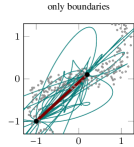
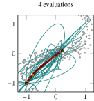
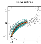
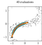
Figure 1: Convergence of probabilistic ODE solver as number of evaluation points increases. Each panel shows a dataset (grey points) whose distribution determines a Riemannian manifold. The algorithm infers the geodesic connecting two points (black) on this manifold. Mean of inferred Gaussian process posterior in red. Evaluation points of the ODE in orange. Green lines are samples drawn from the posterior belief over geodesics. Left-most panel: no ODE evaluations (only boundary values). The supplements contain an animated version of this figure.

3.3 Posterior

After $N$ steps, the algorithm has collected $N$ evaluations $y_{i}=f(\hat{c}_{i},\hat{c}^{\prime}_{i})$, and constructed equally many uncertainty estimates $\Lambda_{i}$. The marginal distribution over the $y_{i}$ under the prior (45) is Gaussian with mean $[\partial^{2}\mu_{c}(t_{1})/\partial t^{2},\dots,\partial^{2}\mu_{c}(t_{N})/\partial t^{2}]^{\intercal}$ and covariance

$$\Gamma :=V\otimes k^{(4)}_{TT}+\Lambda$$ (19)

$$\text{where}\quad k^{(4)}_{TT} \in\mathbb{R}^{N\times N}\quad\text{with}\quad k^{(4)}_{TT,ij}=\frac{\partial^{4}k(t_{i},t_{j})}{\partial t_{i}^{2}\partial t_{j}^{2}}.$$

The matrix $\Lambda\in\mathbb{R}^{DN\times DN}$ is a rearranged form of the block diagonal matrix whose $N$-th block diagonal element is the matrix $\Lambda_{i}\in\mathbb{R}^{D\times D}$. The posterior distribution over $c$, and the output of the algorithm, is thus a Gaussian process with mean function

$$\mu_{c\,|\,a,b,Y}(t)=\mu_{c}(t)+\left[V\otimes\begin{pmatrix}k_{t0}&k_{t1}&k^{\prime\prime}_{tT}\end{pmatrix}\right]\cdot\\ \underbrace{\left[V\otimes\begin{pmatrix}k_{00}&k_{01}&k^{\prime\prime}_{0T}\\ k_{10}&k_{11}&k^{\prime\prime}_{1T}\\ k^{\prime\prime}_{T0}&k^{\prime\prime}_{T1}&k^{(4)}_{TT}\end{pmatrix}+\begin{pmatrix}\Delta_{a}&0&0\\ 0&\Delta_{b}&0\\ 0&0&\Lambda\end{pmatrix}\right]^{-1}}_{=:\Gamma^{-1}}\\ \cdot\begin{bmatrix}a-\mu_{c}(0)&b-\mu_{c}(1)&Y-\mu^{\prime\prime}_{c}(T)\end{bmatrix}^{\intercal}$$ (23)

(where $k^{\prime\prime}_{0t_{j}}=\partial k(0,t_{j})/\partial t_{j}^{2}$, etc.) and covariance function (see also supplements)

$$\operatorname{cov}(c(t_{1}),c(t_{2})\,|\,a,b,Y)=V\otimes k_{t_{1},t_{2}}\\ -\left[V\otimes\begin{pmatrix}k_{t0}&k_{t1}&k^{\prime\prime}_{tT}\end{pmatrix}\right]\Gamma^{-1}\left[V\otimes\begin{pmatrix}k_{0t_{2}}\\ k_{1t_{2}}\\ k^{\prime\prime}_{Tt_{2}}\end{pmatrix}\right].$$ (26)

Fig. 1 shows conceptual sketches. Crucially, this posterior is a joint distribution over the entire curve, not just about its value at a particular value along the curve. This sets it apart from the error bounds returned by classic ODE solvers, and means it can be used directly for Riemannian statistics (Sec. 4).

3.3.1 Iterative Refinements

We have found empirically that the estimates of the method can be meaningfully (albeit not drastically) improved by a small number of iterations over the estimates $\hat{c}_{i},\hat{c}^{\prime}_{i}$ after the first round, without changing the Gram matrix $\Gamma$. In other words, we update the mean estimates used to construct $\hat{c},\hat{c}^{\prime}$ based on the posterior arising from later evaluations. This idea is related to the idea behind implicit Runge-Kutta methods (Hairer et al., 1987, §II.7). It is important not to update $\Gamma$ based on the posterior uncertainty in this process; this would lead to strong over-fitting, because it ignores the recursive role earlier evaluation play in the construction of later estimates.

3.4 Choice of Hyperparameters and Evaluation Points

The prior definitions of Eq. (45) rely on two hyperparameters $V$ and $\lambda$. The output covariance $V$ defines the overall scale on which values $c(t)$ are expected to vary. For curves within a dataset $x_{1:P}\in\mathbb{R}^{D}$, we assume that the curves are typically limited to the Euclidean domain covered by the data, and that geodesics connecting points close within the dataset typically have smaller absolute values than those geodesics connecting points far apart within the dataset. For curves between $a,b$, we thus set $V$ in an empirical Bayesian fashion to $V=\left[(a-b)^{\intercal}S_{x}(a-b)\right]\cdot S_{x}\in\mathbb{R}^{D\times D}$, where $S_{x}$ is the sample covariance of the dataset $x_{1:P}$. For IVPs, we replace $(a-b)$ in this expression by $v$.

The width $\lambda$ of the covariance function controls the regularity of the inferred curve. Values $\lambda\ll 1$ give rise to rough estimates associated with high posterior uncertainty, while $\lambda\gg 1$ gives regular, almost-straight curves with relatively low posterior uncertainty. Following a widely adapted approach in Gaussian regression (Rasmussen and Williams, 2006, §5.2), we choose $\lambda$ to maximise its marginal likelihood under the observations $Y$. This marginal is Gaussian. Using the Gram matrix $\Gamma$ from Eq. (36), its logarithm is

$$-2\log p(Y,a,b\,|\,\lambda)=\begin{pmatrix}a-\mu_{c}(0)\\ b-\mu_{c}(1)\\ Y-\mu^{\prime\prime}_{c}(T)\end{pmatrix}^{\intercal}\Gamma^{-1}\begin{pmatrix}a-\mu_{c}(0)\\ b-\mu_{c}(1)\\ Y-\mu^{\prime\prime}_{c}(T)\end{pmatrix}\\ +\log|\Gamma|+(2+N)\log 2\pi.$$ (29)

A final design choice is the location of the evaluation points $t_{i}$. The optimal choice of the grid points depends on $f$ and is computationally prohibitive, so we use a pre-determined grid. For BVP’s, we use sigmoid grids such as $t_{i}=0.5(1+\operatorname{erf}(-1.5+3i/N))$ as they emphasise boundary areas; for IVP’s we use linear grids. But alternative choices give acceptably good results as well.

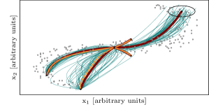
Figure 2: Solving five BVPs within a dataset (grey points). Orange: solutions found by Matlab’s bvp5c. For the probabilistic solver, 30 posterior samples (thin green), and mean as thick red line. Simpler short curves lead to confident predictions, while the challenging curve to the bottom left has drastic uncertainty. Top right curve demonstrates the ability, not offered by classic methods, to deal with uncertain boundary values (the black ellipse represents two standard deviations).

Cost

Because of the inversion of the $((N+2)D)\times((N+2)D)$ matrix $\Gamma$ in Eq. (36), the method described here has computational cost $\mathcal{O}(D^{3}N^{3})$. This may sound costly. However, both $N$ and $D$ are usually small numbers for problems in Riemannian statistics. Modern ODE solvers rely on a number of additional algorithmic steps to improve performance, which lead to considerable computational overhead. Since point estimates require high precision, the computational cost of existing methods is quite high in practice. We will show below that, since probabilistic estimates can be marginalised within statistical calculations, our algorithm in fact improves computation time.

3.5 Relationship to Runge-Kutta methods

The idea of iteratively constructing estimates for the solution and using them to extrapolate may seem ad hoc. In fact, the step from the established Runge-Kutta (RK) methods to this probabilistic approach is shorter than one might think. RK methods proceed in extrapolation steps of length $h$. Each such step consists of $N$ evaluations $y_{i}=f(\hat{c}_{i},t_{i})$. The estimate $\hat{c}_{i}$ is constructed by a linear combination of the previous evaluations and the initial values: $\hat{c}_{i}=w_{0}c_{0}+\sum_{j=1}^{i-1}w_{j}y_{j}$. This is exactly the structure of the mean prediction of Eq. (36). The difference lies in the way the weights $w_{j}$ are constructed. For RK, they are constructed carefully such that the error between the true solution of the ODE and the estimated solution is $\mathcal{O}(h^{-N})$. Ensuring this is highly nontrivial, and often cited as a historical achievement of numerical mathematics (Hairer et al., 1987, §II.5). In the Gaussian process framework, the $w_{i}$ arise much more straightforwardly, from Eq. (36), the prior choice of kernel, and a (currently ad hoc) exploration strategy in $t$. The strength of this is that it naturally gives a probabilistic generative model for solutions, and thus various additional functionality. The downside is that, in this simplistic form, the probabilistic solver can not be expected to give the same local error bounds as RK methods. In fact one can readily construct examples where our specific form of the algorithm has low order. It remains a challenging research question whether the frameworks of nonparametric regression and Runge-Kutta methods can be unified under a consistent probabilistic concept.

4 Probabilistic Calculations on Riemannian Manifolds

We briefly describe how the results from Sec. 3 can be combined with the concepts from Sec. 2 to define tools for Riemannian statistics that marginalise numerical uncertainty of the solver.

Exponential maps

Given an initial point $a\sim\mathcal{N}(\bar{a},\Sigma_{a})$ and initial direction $v\sim\mathcal{N}(\bar{v},\Sigma_{v})$, the exponential map can be computed by solving an IVP (3) as described in Sec. 3. This makes direct use of the ability of the solver to deal with uncertain boundary and initial values.

Logarithm maps

The logarithm map (4) is slightly more complicated to compute as the length of a geodesic cannot be computed linearly. We can, however, sample from the logarithm map as follows. Let $a\sim\mathcal{N}(\bar{a},\Sigma_{a})$ and $b\sim\mathcal{N}(\bar{b},\Sigma_{b})$ and construct the geodesic Gaussian process posterior. Sample $c_{s}$ and $c_{s}^{\prime}$ from this process and compute the corresponding logarithm map using Eq. (4). The length of $c_{s}$ is evaluated using standard quadrature. The mean and covariance of the logarithm map can then be estimated from the samples. Resorting to a sampling method might seem expensive, but in practice the runtime is dominated by the BVP solver.

Computing Means

The mean of $x_{1:P}$ is computed using gradient descent (5), so we need to track the uncertainty through this optimisation. Let $\mu_{k}\sim\mathcal{N}(\bar{\mu}_{k},\Sigma_{\mu_{i}})$ denote the estimate of the mean at iteration $i$ of the gradient descent scheme. First, compute the mean and covariance of

$$v=\frac{1}{P}\sum_{i}\mathrm{Log}_{\mu_{k}}(x_{i})$$ (30)

by sampling as above. Assuming $v$ follows a Gaussian distribution with the estimated mean and covariance, we then directly compute the distribution of

$$\mu_{k+1}=\mathrm{Exp}_{\mu_{k}}(\alpha v).$$ (31)

Probabilistic optimisation algorithms (Hennig, 2013), which can directly return probabilistic estimates for the shape of the gradient (5), are a potential alternative.

Computing Principal Geodesics

Given a mean $\mu\sim\mathcal{N}(\bar{\mu},\Sigma_{\mu})$, estimate the mean and covariance of $\mathrm{Log}_{\mu}(x_{1:P})$ and use these to estimate the mean and covariance of the principal direction $v$. The principal geodesic can then be computed as $\gamma=\mathrm{Exp}_{\mu}(v)$.

5 Experiments

        

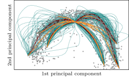
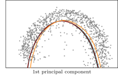
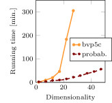
Figure 3: Results on 1000 images of the digit 1 from the MNIST handwritten digits data set, projected into its first two principal components. Left: Several geodesics from the mean computed using the probabilistic solver (red mean predictions, green samples) as well as Matlab’s bvp5c (orange). Middle: The principal geodesics estimated using the same two solvers. Right: Running time of a mean value computation using different solvers as a function of the dimensionality.

This section reports on experiments with the suggested algorithms. It begins with an illustrative experiment on the well-known MNIST handwritten data set, followed by a study of the running time of the algorithms on the same data. Finally, we use the algorithms for visualising changes in human body shape.

5.1 Handwritten Digits

Fig. 3 (next page, for layout reasons), left and centre, show 1000 images of the digit 1 expressed in the first two principal components of the data. This data roughly follows a one-dimensional nonlinear structure, which we estimate using PGA. To find geodesics that follow the local structure of the data, we learn local metric tensors as local inverse covariance matrices, and combine them to form a smoothly changing metric using Eq. 7. The local metric tensors are learned using a standard EM algorithm for Gaussian mixtures (McLachlan and Krishnan, 1997).

For comparison, we consider a state-of-the-art BVP solver as implemented in Matlab in bvp5c (a four-stage implicit Runge-Kutta method (Hairer et al., 1987, §II.7)). This does not provide an uncertain output, so we resort to the deterministic Riemannian statistics algorithms (Sec. 2). Fig. 3, left, shows a few geodesics from the mean computed by our solver as well as bvp5c. The geodesics provided by the two solvers are comparable and tend to follow the structure of the data. Fig. 3, centre, shows the principal geodesics of the data computed using the different solvers; the results are comparable. This impression is supported by a more close comparison of the results: Figure 4 shows curve lengths achieved by the two solvers. While bvp5c tends to perform slightly better, in particular for long curves, the error estimates of the probabilistic solvers reflect the algorithm’s imprecision quite well.

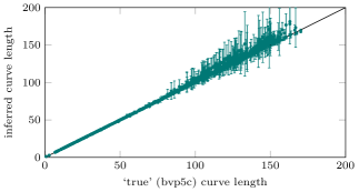
Figure 4: Inferred curve lengths for the 1000 geodesics from Figure 3. The probabilistic estimates for the lengths (mean $\pm$ 2 standard deviations) are plotted against the (assumed reliable) point estimates of Matlab’s bvp5c.

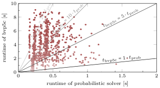
Figure 5: Runtime of bvp5c against that of the probabilistic solver for the same geodesics (note differing abscissa and ordinate scales). The color of points encodes the length of the corresponding curve, from 0 (white) to 200 (dark red), for comparison with Fig. 4.

Even within this simple two-dimensional setting, the running times of the two different solvers can diverge considerably. Figure 5 plots the two runtimes against each other (along with the corresponding curve length, in color). The probabilistic solvers’ slight decrease in precision is accompanied by a decrease in computational cost by about an order of magnitude. Due to its design, the computational cost of the probabilistic solver is almost unaffected by the complexity of the problem (length of the curve). Instead, harder problems simply lead to larger uncertainty. As dimensionality increases, this advantage grows. Fig. 3, right, shows the running time for computations of the mean for an increasing number of dimensions. For this experiment we use 100 images and 5 iterations of the gradient descent scheme. As the plot shows, the probabilistic approach is substantially faster in this experiment.

5.2 Human Body Shape

$\mu-3\sigma$	$\mu$	$\mu+3\sigma$

Figure 6: Samples from the posterior over the principal geodesic through the body shape dataset, estimated under a metric learned to emphasise belly circumference. Six samples each at the inferred manifold mean (centre) and three standard deviations of the dataset in either direction (left, right). The variation is shown in the supplementary video.

We also experimented with human body shape data, using $1191$ laser scans and anthropometric measurements of the belly circumference of female subjects (Robinette et al., 1999). Body shape is represented using a $50$-dimensional SCAPE model (Anguelov et al., 2005), such that each scan is a vector in $\mathbb{R}^{50}$. Following Hauberg et al. (2012a), we partition the subjects in $7$ clusters by belly circumferences, learn a diagonal Large Margin Nearest Neighbour (LMNN) metric (Weinberger and Saul, 2009) for each cluster, and form a smoothly changing metric using Eq. 7. Under this metric variance is inflated locally along directions related to belly circumference. We visualise this increased variance using PGA. Based on the timing results above, we only consider the probabilistic algorithm here, which achieved a runtime of $\sim$10 minutes.

Fig. 6 shows the first principal geodesic under the learned metric, where we show bodies at the mean as well as $\pm$ three standard deviations from the mean. Uncertainty is visualised by six samples from the principal geodesic at each point; this uncertainty is not described by other solvers (this is more easily seen in the supplementary video). In general, the principal geodesic shows an increasing belly circumference (again, see supplementary video).

6 Conclusion

We have studied a probabilistic solver for ordinary differential equations in the context of Riemannian statistics. The method can deal with uncertain boundary and initial values, and returns a joint posterior over the solution. The theoretical performance of such methods is currently not as tightly bounded as that of Runge-Kutta methods, but their structured error estimates allow a closed probabilistic formulation of computations on Riemannian manifolds. This includes marginalisation over the solution space, which weakens the effect of numerical errors. This, in turn, means computational precision, and thus cost, can be lowered. The resulting improvement in computation time and functionality is an example for the conceptual and applied value of probabilistically designed numerical algorithms for computational statistics.

Acknowledgements

S. Hauberg is supported in part by the Villum Foundation as well as an AWS in Education Machine Learning Research Grant award from Amazon.com.

— Supplementary Material —

Appendix A Gaussian Process Posteriors

Equations (10), (12), (18) and (19) in the main paper are Gaussian process posterior distributions over the curve $c$ arising from observations of various combinations of derivatives of $c$. These forms arise from the following general result. Consider a Gaussian process prior distribution

$$p(c)=\mathcal{GP}(c;\mu,k)$$ (34)

over the function $c$, and observations $y$ with the likelihood

$$p(y\,|\,c,A)=\mathcal{N}(y;Ac,\Lambda),$$ (35)

with a linear operator $A$. This includes the special cases of the selection operator $A=\delta(x-x_{i})$ which selects function values $Ac=\int\delta(x-x_{i})c(x)\mathrm{d}x=c(x_{i})$, and the special case of derivative operators $\partial_{x}^{n}\delta(x-x_{i})$ which give $Ac=\int\partial_{x}\delta(x-x_{i})c(x)\mathrm{d}x=c^{(n)}(x_{i})$. Then the posterior over any linear map $Bc$ of the curve $c$ (including $B=\delta(x-x_{j})$, giving $Bc=c(x_{j})$) is

$$p(Bc\,|\,y,A)=\mathcal{GP}(Bc;B\mu+BkA^{\intercal}(AkA^{\intercal}+\Lambda)^{-1}(y-A\mu),BkB-BkA^{\intercal}(AkA^{\intercal}+\Lambda)^{-1}AkB^{\intercal}).$$ (36)

And the marginal probability for $y$ is

$$p(y\,|\,A)=\int p(y\,|\,c,A)p(c)\,dc=\mathcal{N}(y;A\mu,AkA^{\intercal}+\Lambda)$$ (37)

The classic example is that of the marginal posterior at $c(x_{*})$ arising from noisy observations at $[c(x_{1}),\dots,c(x_{N})]^{\intercal}$. This is the case of $B=\delta(x-x_{*})$ and $A=[\delta(x-x_{1}),\dots,\delta(x-x_{N})]^{\intercal}$, which gives

$$B\mu =\mu(x_{*})$$ (38)

$$A\mu =[\mu(x_{1}),\dots\mu(x_{N})]^{\intercal}$$ (39)

$$BkA^{\intercal} =\left[\iint\delta(a-x_{*})k(a,b)\delta(b-x_{i})\,da\,db\right]_{i=1,\dots,N}=[k(x_{*},x_{1}),\dots k(x_{*},x_{N})]$$ (40)

$$AkA^{\intercal} =\begin{pmatrix}k(x_{1},x_{1})&\cdots&k(x_{1},x_{N})\\ \vdots&\ddots&\vdots\\ k(x_{N},x_{1})&\cdots&k(x_{N},x_{N})\end{pmatrix}$$ (41)

and so on. All the Gaussian forms in the paper are special cases with various combinations of $A$ and $B$.

Appendix B Covariance Functions

The models in the paper assume a squared-exponential (aka. radial basis function, Gaussian) covariance function between values of the function $\boldsymbol{f}:\mathbb{R}\operatorname*{\rightarrowtriangle}\mathbb{R}^{N}$, of the form

$$\operatorname{cov}(f_{i}(t),f_{j}(t^{\prime}))=V_{ij}\exp\left(-\frac{(t-t^{\prime})^{2}}{2\lambda^{2}}\right)\equalscolon V_{ij}k_{tt^{\prime}}$$ (42)

The calculations require the covariance between various combinations of derivatives of the function. For clear notation, we’ll use the operator $\partial\colonequals\partial/\partial t$, and the abbreviation $\delta_{tt^{\prime}}\colonequals(t-t^{\prime})/\lambda^{2}$

$$\operatorname{cov}(f_{i}(t),\dot{f}_{j}(t^{\prime})) =V_{ij}k_{tt^{\prime}}\partial^{\intercal}=V_{ij}\frac{t-t^{\prime}}{\lambda^{2}}k_{tt^{\prime}}=V_{ij}\delta_{tt^{\prime}}k_{tt^{\prime}}=-\operatorname{cov}(\dot{f}_{i}(t),f_{j}(t^{\prime}))$$ (43)

$$\operatorname{cov}(\dot{f}_{i}(t),\dot{f}_{j}(t^{\prime})) =V_{ij}\partial k_{tt^{\prime}}\partial^{\intercal}=V_{ij}\left(\frac{1}{\lambda^{2}}-\left(\frac{t-t^{\prime}}{\lambda^{2}}\right)^{2}\right)k_{tt^{\prime}}=V_{ij}\left(\frac{1}{\lambda^{2}}-\delta^{2}_{tt^{\prime}}\right)k_{tt^{\prime}}$$ (44)

$$\operatorname{cov}(f_{i}(t),\ddot{f}_{j}(t^{\prime})) =V_{ij}k_{tt^{\prime}}\partial^{\intercal}\partial^{\intercal}=V_{ij}\left(\left(\frac{t-t^{\prime}}{\lambda^{2}}\right)^{2}-\frac{1}{\lambda^{2}}\right)k_{tt^{\prime}}=V_{ij}\left(\delta^{2}_{tt^{\prime}}-\frac{1}{\lambda^{2}}\right)k_{tt^{\prime}}=-\operatorname{cov}(\dot{f}_{i}(t),\dot{f}_{j}(t^{\prime}))$$ (45)

$$\operatorname{cov}(\dot{f}_{i}(t),\ddot{f}_{j}(t^{\prime})) =V_{ij}\partial k_{tt^{\prime}}\partial^{\intercal}\partial^{\intercal}=V_{ij}\left(\frac{2}{\lambda^{2}}\frac{t-t^{\prime}}{\lambda^{2}}-\frac{t-t^{\prime}}{\lambda^{2}}\left(\left(\frac{t-t^{\prime}}{\lambda^{2}}\right)^{2}-\frac{1}{\lambda^{2}}\right)\right)k_{tt^{\prime}}=V_{ij}\left(-\delta^{3}_{tt^{\prime}}+\frac{3}{\lambda^{2}}\delta_{tt^{\prime}}\right)k_{tt^{\prime}}$$ (46)

$$\operatorname{cov}(\ddot{f}_{i}(t),\ddot{f}_{j}(t^{\prime})) =V_{ij}\partial\partial k_{tt^{\prime}}\partial^{\intercal}\partial^{\intercal}=V_{ij}\left(\delta^{4}_{tt^{\prime}}-\frac{6}{\lambda^{2}}\delta^{2}_{tt^{\prime}}+\frac{3}{\lambda^{4}}\right)k_{tt^{\prime}}$$ (47)

Of course, all those derivatives retain the Kronecker structure of the original kernel, because $\partial(V\otimes k)=V\otimes\partial k$.

Appendix C Inferring Hyperparameters

Perhaps the most widely used way to learn hyperparameters for Gaussian process models it type-II maximum likelihood estimation, also known as evidence maximisation: The marginal probability for the observations $y$ is $p(y\,|\,\lambda)=\int p(y\,|\,c)p(c\,|\,\lambda)\>dc=\mathcal{N}(y;\ddot{\mu}_{T},\partial\partial k_{TT}(\lambda)\partial\partial+\Lambda)$. Using the shorthand $G:=(\partial\partial k_{TT}(\lambda)\partial\partial+\Lambda)$, its logarithm is

$$-2\log p(y\,|\,\lambda)=(y-\ddot{\mu}_{T})^{\intercal}G^{-1}(y-\ddot{\mu}_{T})+\log|G|+N\log 2\pi$$ (48)

To optimise this expression with respect to the length scale $\lambda$, we use

$$-2\frac{\partial\log p(y\,|\,\lambda)}{\partial\lambda^{2}}=-(y-\ddot{\mu}_{T})^{\intercal}G^{-1}\frac{\partial G}{\partial\lambda^{2}}G^{-1}(y-\ddot{\mu}_{T})+\operatorname{tr}(G^{-1}\frac{\partial G}{\partial\lambda^{2}}).$$ (49)

From Equation (47), and using

$$\frac{\partial\delta_{tt^{\prime}}}{\partial\lambda^{2}}=-\frac{\delta_{tt^{\prime}}}{\lambda^{2}}\qquad\qquad\frac{\partial k_{tt^{\prime}}}{\partial\lambda^{2}}=k_{tt^{\prime}}\frac{\delta^{2}_{tt^{\prime}}}{2}$$ (50)

we find

$$\frac{\partial G^{ij}_{tt^{\prime}}}{\partial\lambda^{2}} =V_{ij}\left[\left(-\frac{4}{\lambda^{2}}\delta^{4}_{tt^{\prime}}+\frac{18}{\lambda^{4}}\delta^{2}_{tt^{\prime}}+\frac{6}{\lambda^{6}}\right)k_{tt^{\prime}}+\partial\partial k_{tt^{\prime}}\partial^{\intercal}\partial^{\intercal}\frac{\delta_{tt^{\prime}}^{2}}{2}\right]$$ (51)

$$=V_{ij}\left(\frac{\delta^{6}}{2}-\frac{7}{\lambda^{2}}\delta^{4}_{tt^{\prime}}+\frac{39}{2\lambda^{4}}\delta^{2}_{tt^{\prime}}+\frac{6}{\lambda^{6}}\right)k_{tt^{\prime}}$$ (52)

It is also easy to evaluate the second derivative, giving

$$-2\frac{\partial^{2}\log p(y\,|\,\lambda)}{(\partial\lambda^{2})^{2}} =2(y-\ddot{\mu}_{T})^{\intercal}G^{-1}\frac{\partial G}{\partial\lambda^{2}}G^{-1}\frac{\partial G}{\partial\lambda^{2}}G^{-1}(y-\ddot{\mu}_{T})-\operatorname{tr}\left[\frac{\partial G}{\partial\lambda^{2}}G^{-1}\frac{\partial G}{\partial\lambda^{2}}G^{-1}\right]$$ (53)

$$-(y-\ddot{\mu}_{T})^{\intercal}G^{-1}\frac{\partial^{2}G}{(\partial\lambda^{2})^{2}}G^{-1}(y-\ddot{\mu}_{T})+\operatorname{tr}\left[G^{-1}\frac{\partial^{2}G}{(\partial\lambda^{2})^{2}}\right]$$ (54)

$$\text{where}\qquad\frac{\partial^{2}G^{ij}_{tt^{\prime}}}{(\partial\lambda^{2})^{2}} =V_{ij}\left(-\frac{3}{\lambda^{2}}\delta_{tt^{\prime}}^{6}+\frac{35}{\lambda^{4}}\delta_{tt^{\prime}}^{4}-\frac{78}{\lambda^{6}}\delta_{tt^{\prime}}^{2}+\frac{18}{\lambda^{8}}\right)k_{tt^{\prime}}+\frac{\delta^{2}}{2}\frac{\partial G_{tt^{\prime}}^{ij}}{\partial\lambda^{2}}$$ (55)

This allows constructing a Newton-Raphson optimisation scheme for the length scale of the algorithm.

References

- Anguelov et al. [2005] D. Anguelov, P. Srinivasan, D. Koller, S. Thrun, J. Rodgers, and J. Davis. Scape: shape completion and animation of people. ACM Transactions on Graphics, 24(3):408–416, 2005.
- Berger [2007] M. Berger. A Panoramic View of Riemannian Geometry. Springer, 2007.
- Chkrebtii et al. [2013] O. Chkrebtii, D.A. Campbell, M.A. Girolami, and B. Calderhead. Bayesian uncertainty quantification for differential equations. arXiv, stat.ME 1306.2365, June 2013.
- Diaconis [1988] P. Diaconis. Bayesian numerical analysis. Statistical decision theory and related topics, IV(1):163–175, 1988.
- Fletcher et al. [2004] P.T. Fletcher, C. Lu, S.M. Pizer, and S. Joshi. Principal Geodesic Analysis for the study of Nonlinear Statistics of Shape. IEEE Transactions on Medical Imaging, 23(8):995–1005, 2004.
- Freifeld and Black [2012] O. Freifeld and M.J. Black. Lie bodies: A manifold representation of 3D human shape. In A. Fitzgibbon et al., editor, European Conf. on Computer Vision (ECCV), Part I, LNCS 7572, pages 1–14. Springer-Verlag, oct 2012.
- Hairer et al. [1987] E. Hairer, S.P. Nørsett, and G. Wanner. Solving Ordinary Differential Equations I – Nonstiff Problems. Springer, 1987.
- Hauberg et al. [2012a] S. Hauberg, O. Freifeld, and M.J. Black. A geometric take on metric learning. In P. Bartlett, F.C.N. Pereira, C.J.C. Burges, L. Bottou, and K.Q. Weinberger, editors, Advances in Neural Information Processing Systems (NIPS) 25, pages 2033–2041. MIT Press, 2012a.
- Hauberg et al. [2012b] S. Hauberg, S. Sommer, and K.S. Pedersen. Natural metrics and least-committed priors for articulated tracking. Image and Vision Computing, 30(6-7):453–461, 2012b.
- Hennig [2013] P. Hennig. Fast probabilistic optimization from noisy gradients. In Proceedings of the 30th International Conference on Machine Learning (ICML), 2013.
- Kutta [1901] W. Kutta. Beitrag zur näherungsweisen Integration totaler Differentialgleichungen. Zeitschrift für Mathematik und Physik, 46:435–453, 1901.
- McLachlan and Krishnan [1997] G.J. McLachlan and T. Krishnan. The EM Algorithm and its Extensions. Wiley, 1997.
- O’Hagan [1992] A. O’Hagan. Some Bayesian numerical analysis. Bayesian Statistics, 4:345–363, 1992.
- Pennec [1999] X. Pennec. Probabilities and statistics on Riemannian manifolds: Basic tools for geometric measurements. In Proceedings of Nonlinear Signal and Image Processing, pages 194–198, 1999.
- Porikli et al. [2006] F. Porikli, O. Tuzel, and P. Meer. Covariance tracking using model update based on Lie algebra. In IEEE Computer Society Conference on Computer Vision and Pattern Recognition (CVPR), volume 1, pages 728–735. IEEE, 2006.
- Rasmussen and Williams [2006] C.E. Rasmussen and C.K.I. Williams. Gaussian Processes for Machine Learning. MIT Press, 2006.
- Robinette et al. [1999] K.M. Robinette, H. Daanen, and E. Paquet. The CAESAR project: a 3-D surface anthropometry survey. In 3-D Digital Imaging and Modeling, pages 380–386, 1999.
- Runge [1895] C. Runge. Über die numerische Auflösung von Differentialgleichungen. Mathematische Annalen, 46:167–178, 1895.
- Skilling [1991] J. Skilling. Bayesian solution of ordinary differential equations. Maximum Entropy and Bayesian Methods, Seattle, 1991.
- Tenenbaum and Pollard [1963] M. Tenenbaum and H. Pollard. Ordinary Differential Equations. Dover Publications, 1963.
- van Loan [2000] C.F. van Loan. The ubiquitous Kronecker product. J of Computational and Applied Mathematics, 123:85–100, 2000.
- Weinberger and Saul [2009] K.Q. Weinberger and L.K. Saul. Distance metric learning for large margin nearest neighbor classification. The Journal of Machine Learning Research, 10:207–244, 2009.