SEJONG OPEN CLUSTER SURVEY (SOS).
0. TARGET SELECTION AND DATA ANALYSIS

Abstract

Star clusters are superb astrophysical laboratories containing cospatial and coeval samples of stars with similar chemical composition. We have initiated the Sejong Open cluster Survey (SOS) - a project dedicated to providing homogeneous photometry of a large number of open clusters in the SAAO Johnson-Cousins’ $UBVI$ system. To achieve our main goal, we have paid much attention to the observation of standard stars in order to reproduce the SAAO standard system.
Many of our targets are relatively small, sparse clusters that escaped previous observations. As clusters are considered building blocks of the Galactic disk, their physical properties such as the initial mass function, the pattern of mass segregation, etc. give valuable information on the formation and evolution of the Galactic disk. The spatial distribution of young open clusters will be used to revise the local spiral arm structure of the Galaxy. In addition, the homogeneous data can also be used to test stellar evolutionary theory, especially concerning rare massive stars. In this paper we present the target selection criteria, the observational strategy for accurate photometry, and the adopted calibrations for data analysis such as color-color relations, zero-age main sequence relations, Sp - M_V relations, Sp - T_eff relations, Sp - color relations, and T_eff - BC relations. Finally we provide some data analysis such as the determination of the reddening law, the membership selection criteria, and distance determination.

1 INTRODUCTION

Open clusters are stellar systems containing a few (100 – 1000) coeval stars with nearly the same chemical composition. They are ideal targets to test stellar evolution theory. As open clusters are stellar systems, they provide valuable information on the distance and age of stars in the cluster, information that is very difficult to obtain from field stars. In contrast to globular clusters, open clusters have a wide range of ages. As they are important building blocks of the Galactic disk, the distribution of age and abundance of open clusters provide information on the star formation history in the Galaxy. In addition, the stellar initial mass function (IMF) from open clusters is one of the basic ingredients in constructing the star formation history of the Galaxy as well as the population synthesis of unresolved remote galaxies.

The number of known open clusters is about 1700, but some seem to be not real clusters (Cheon et al. 2010) and some may be remnants of disrupted clusters. Owing to several all sky surveys such as Hipparcos, Tycho, 2MASS, etc, many new open clusters or associations were identified (Bica et al. 2003; Dutra et al. 2003; Karachenko et al. 2005). Open clusters can be classified into three groups according to their age (Sung 1995) – young (age $\mathrel{\hbox{\hbox to0.0pt{\hbox{\lower 4.0pt\hbox{$\sim$}}\hss}\hbox{$<$}}}10^{7}$ yrs), intermediate-age (age: $10^{7}$ – $7\times 10^{8}$ yrs), and old (age $\mathrel{\hbox{\hbox to0.0pt{\hbox{\lower 4.0pt\hbox{$\sim$}}\hss}\hbox{$>$}}}7\times 10^{8}$ yrs). Young open clusters can give information on the stellar evolution of massive stars (Conti et al. 1983; Massey 2003; Kook et al. 2010; Lim et al. 2013) as well as on low-mass pre-main sequence (PMS) stars (Sung et al. 1997; Luhman 2012). As massive stars are still in the main sequence (MS) or in evolved stages, young open clusters are ideal targets for studying the stellar IMF in a wide mass range (Sung & Bessell 2004; Sung et al. 2004; Sung & Bessell 2010). In addition, as they are still in or near their birthplace, the spiral arm structure of the Galaxy can be derived from the spatial distribution of young open clusters. Typical young open clusters are the Trapezium cluster (or the Orion Nebula Cluster, ONC), NGC 2264 and NGC 2244 in Moncerotis, IC 1805 and IC 1848 in Cassiopeia, NGC 6231 in Scorpius, NGC 6530 (M8) and M20 (the Trifid nebula) in Sagittarius, NGC 6611 (the Eagle nebula) in Serpens, Trumpler 14 (Tr 14), Tr 15, Tr 16, Collinder 228 (Cr 228), and Cr 232 in the $\eta$ Carina nebula. The double cluster h & $\chi$ Per is slightly older than the clusters listed above, but they are still classified as young open clusters.

As old open clusters are considered representative of the first generation of stars in the Galactic disk, they can give information on the star formation history in the Galactic disk and the chemical evolution of the Galaxy (Kim et al. 2003). As an open cluster is a stellar system, stars in the cluster are subject to dynamical evolution (Sung et al. 1999). As their age is older than the typical relaxation time scale of open clusters, intermediate-age and old open clusters are good laboratories for testing the dynamical evolution of multi-mass systems. Typical intermediate-age open clusters are the Pleiades and Hyades in Taurus, Praesepe in Cancer, M35 in Gemini, and M11 in Scutum. Typical old clusters are M67, NGC 188, and NGC 6971.

Lada & Lada (2003) and Porras et al. (2003) found that about 80% of the stars in star forming regions in the Solar neighborhood are in clusters with at least 100 members. As small clusters or groups are dynamically unbound, the stars in small clusters and groups will disperse and become the field stars in the Galactic disk. Unfortunately, as most observations are mainly focused on relatively rich open clusters, we have not much information on these small clusters. In addition, the number of stars in such small clusters is insufficient to test reliably stellar evolution theory, as well as dynamical evolution models. These obstacles can be overcome by combining data for several open clusters with a similar age. This is the importance of the open cluster survey project.

Many photometric surveys of open clusters have been conducted up to now. Among them “Photometry of stars in Galactic cluster field” (Hoag et al. 1961) was the first comprehensive photoelectric and photographic photometry of open clusters in the Northern hemisphere. In the 1970s, N. Vogt and A. F. J. Moffat performed $UBV$ & H$\beta$ photoelectric photometry of many young open clusters in the Southern hemisphere (Vogt & Moffat 1972, 1973; Moffat & Vogt 1973a, 1975a, 1975b, 1975c) and in the l = 135^∘ region (Moffat & Vogt 1973b).

As the photon collecting area of CCDs increased rapidly in the 2000s, several photometric surveys of open clusters based on CCD photometry were started. Photometric surveys of open clusters in the 1990s were performed by several researchers (see Ann et al. (1999) for a summary). K. A. Janes and R. L. Phelps performed photometric surveys of open clusters in the Northern hemisphere (janes93; phelps94). Ann et al. (1999, 2002) started the BOAO Photometric Atlas of Open Clusters with the Bohyun-san Optical Astronomy Observatory (BOAO) 1.8m telescope to understand the structure of clusters and of the Galactic disk. They selected 343 target clusters and ambitiously started the project, but because of poor weather conditions in Korea, only two papers (photometric data for 16 clusters) were published from the survey project. The CFHT Open Star Cluster Survey (Kalirai et al. 2001a, b, c) selected and observed 19 intermediate-age open clusters, but the survey team published deep photometric data for only 4 open clusters. The WIYN Open Cluster Study (WOCS) (Mathieu 2000) is the most successful open cluster survey program up to now. The WOCS team selected cluster members from deep photometry, spectroscopic radial velocity surveys, and proper motion studies. They studied binarity, stellar activity, chemical composition as well as observational tests of stellar evolution theory. The Bologna Open Cluster Chemical Evolution Project (Bragaglia & Tosi 2006) published photometric data for 16 open clusters obtained with 1m to 4m-class telescopes. Recently Maciejewski & Niedzielski (2007) published $BV$ photometric data for 42 open clusters, but their data are very shallow due to the small aperture size of the telescope and shows a large scatter probably due to bad weather.

We have started the Sejong Open cluster Survey (hereafter SOS) (Lim et al. 2011), a project dedicated to provide homogeneous photometry of a large number of open clusters in the Johnson-Cousins’ $UBVI$ system which is tightly matched to the SAAO standard $UBVRI$ system. To achieve our main goal we will pay much attention to the observation of standard stars in order to reproduce the SAAO standard system (Menzies et al. 1989, 1991; Kilkenny et al. 1998). We have already derived the standard transformation relations for the AZT-22 1.5m telescope at Maidanak Astronomical Observatory (MAO) in Uzbekistan (Lim et al. 2009), for the Kuiper 61^′′ on Mount Bigelow, Arizona, USA (Lim et al. 2013, in preparation), as well as for the 1m telescope at Siding Spring Observatory (SSO) (Sung & Bessell 2000).

The homogeneous photometric data from this project can be used in the study of
(1) the local spiral arm structure of the Galaxy
(2) the observational test of stellar evolution theory
(3) the stellar IMF
(4) the dynamical evolution of star clusters
(5) the star formation history of the Galaxy
(6) the chemical evolution of the Galaxy

In Section 2, we will describe the target selection criteria, and the spatial distribution of target clusters. In Section 3, we describe our strategy for accurate photometry such as determination of the atmospheric extinction coefficients, transformation coefficients, and correction for the other factors affecting photometry. In Section 4, we adopt several calibrations required for the analysis of photometric data such as the intrinsic color relations, zero-age main sequence (ZAMS) relations, the Spectral Type (Sp) - M_V relation, the Sp - T_eff relation, etc. In Section 5, we present some data analysis such as the determination of the reddening law, the membership selection criteria, and distance determination. We summarize our main results in Section 6.

2 TARGET SELECTION

2.1 Status of Open Cluster Data

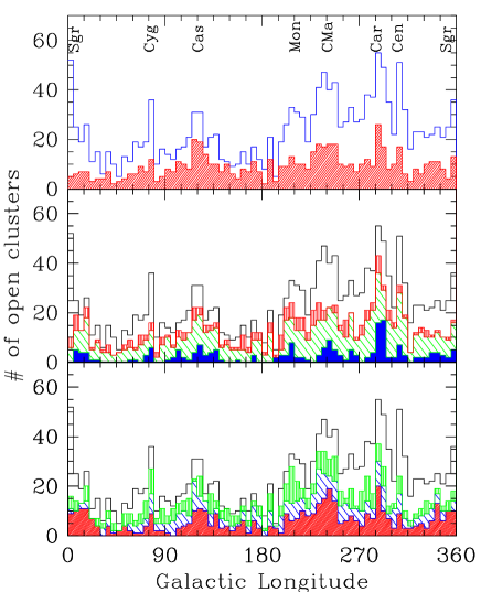
Fig. 1.—: Distribution of open clusters with Galactic longitude. (Top) Open histogram: number of all open clusters at a given longitude bin. Red hatched histogram: number of open clusters observed in the $UBV$ photometric system. (Middle) Distribution of open clusters according to their age – blue: young open clusters, green: intermediate-age open clusters, red: old open clusters, white: unknown. (Bottom) Distribution of open clusters according to the survey priority (see Section 2.2). – red: priority 1, blue: priority 2, green: priority 3, white: priority 4.

After the introduction of CCDs in astronomy, most observations were focused on densely populated clusters, globular clusters, or external galaxies, and the observational status of relatively poor open clusters was largely neglected. Among 1686 open clusters listed in the open cluster data base WEBDA, about 550 clusters were observed either by means of $UBV$ photoelectric photometry or modern CCD photometry, i.e. two thirds of the listed open clusters have still not been observed even in the $UBV$ system. Firstly, we checked photometric data of all the open clusters in WEBDA. The spatial distribution and the observational status of open clusters versus Galactic longitude are shown in Figure 1.

Until now several open cluster survey projects have been performed or are in progress. In order to derive meaningful results from the combined photometric data of open clusters with a similar age, the most important factor is the homogeneity of the photometry. Unfortunately, some photometric data show large deviations (see Mermilliod & Paunzen (2003) or Figure 2). The size of the deviations is much larger than the expected errors from uncertainty in atmospheric extinction correction. The large systematic differences shown in Figure 2 seem to be caused by errors, either in the atmospheric extinction correction or in the transformation to the standard system, or both.

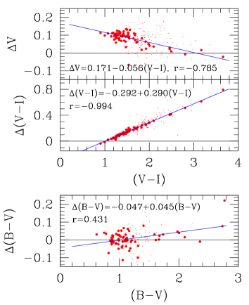
Fig. 2.—: Comparison of the photometry presented by Kook et al. (2010) with that of Piatti & Clariá (2001) for the stars in the young open cluster Hogg 15. Large and small dots represent bright ($V\leq 17$ mag) and faint stars ($V>17$ mag), respectively. There are large systematic differences in $V$ and $V-I$ between Kook et al. (2010) and Piatti & Clariá (2001), but the difference in $B-V$ is not so pronunced.

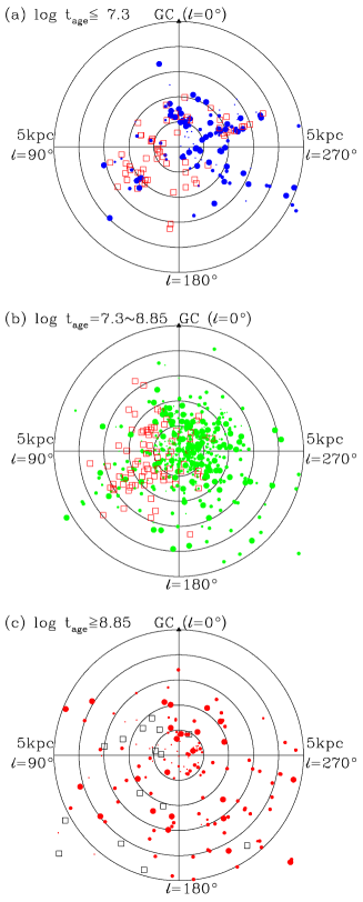
Fig. 3.—: Distribution of target clusters projected on the Galactic plane. The size of dots represents the priority of observation, and the square represents the open clusters already observed. (Upper) Distribution of young open clusters. (Middle) Distribution of intermediate-age open clusters. (Lower) Distribution of old open clusters.

We started a project to observe a large number of open clusters in both the Southern and northern hemispheres. We observed several open clusters in the nouthern hemisphere with the 1m telescope at SSO, and observed more open clusters with the 1m telescope at CTIO in 2011. In addition, we have obtained the images of many Northern open clusters using the AZT-22 1.5m telescope at MAO in Uzbekistan over 5 years from August 2004. We discovered that the atmospheric extinction coefficients at MAO are very high during the summer season due to dust from the desert. Those in fall and winter are normal. We are observing more open clusters in the northern hemisphere with the Kuiper 61^′′ telescope in Arizona, USA from October 2011.

2.2 Target Selection Criteria

We downloaded a $\sim 15^{\prime}\times 15^{\prime}$ image for most of the open clusters from the STSci Digitized Sky Survey, and checked all the images visually. The target selection criteria are
- priority 1 : young open clusters or dense open clusters with no $UBVI$ data
- priority 2 : relatively dense open clusters without $UBVI$ data or well-observed open clusters for the homogeneity of photometry
- priority 3 : sparse open clusters
- priority 4 : no clustering of stars.

We have selected 455, 318, 318, and 604 clusters with priority 1, 2, 3, and 4, respectively. Among them, 125 priority 1 targets, 47 priority 2 targets, 15 priority 3 targets, and 10 priority 4 targets have been observed with the telescopes listed above (up to February 2013). The spatial distributions of selected clusters with Galactic longitude is in the bottom panel of Figure 1. We also plotted the spatial distribution of open clusters projected onto the Galactic plane for three age groups in Figure 3. In the upper panel, we limited the open clusters to those younger than 20 Myr because the age of many young open clusters was assigned to be about 10 Myr. The local spiral arm structure can clearly be seen in the upper panel, and is barely visible in the middle panel. The old open clusters are distributed evenly in the plane. Currently more than half of the priority 1 targets in the Northern hemisphere have been observed, and we are now searching for a 1m-class telescope in the Southern hemisphere.

3 OBSERVATION STRATEGY

To perform accurate photometry, we should pay as much attention to the preparation of the observations as to the observation of standard stars. It is well-known that there are some systematic differences between the Landolt standard $UBVRI$ system (Landolt 1992) and the SAAO $UBVRI$ system (Menzies et al. 1989, 1991; Bessell 1995). Hence, it is important to have some knowledge of the photometric system. Without knowledge of the characteristics of an observing site and of the photometric system, it is impossible to achieve 1% error levels in photometry.

3.1 Standard Stars

The selection of standard stars is one of the most important aspects within the standard system photometry. We found the necessity of a non-linear correction term in the transformation to the Landolt (1992) $U$ system (Sung et al. 1998; Sung & Bessell 2000). To avoid this and to obtain accurate standardized data in $U-B$, we observed the SAAO secondary standard Equatorial stars (Menzies et al. 1991) and the extremely blue and red stars from Kilkenny et al. (1998). Unfortunately, most of these stars are very bright, and we have to use short exposure times for them. We carefully check for uneven illumination patterns or systematic differences in the effective exposure time for the images obtained with short exposures ($\tau_{exp}\mathrel{\hbox{\hbox to0.0pt{\hbox{\lower 4.0pt\hbox{$\sim$}}\hss}\hbox{$<$}}}10$ s, see for example Lim et al. (2008)).

3.2 Extinction Coefficients

Atmospheric extinction is caused by absorption and scattering by air molecules or other particles in the Earth’s atmosphere. Most of the extinction in the visual window is due to Rayleigh scattering ($\propto{1\over\lambda^{4}}$) by air molecules. Another important and variable contributor to the extinction is the scattering and absorption by small liquid or solid particles of various sizes called aerosols (Cousins & Caldwell 1998). The total extinction value depends primarily on the line-of-sight length through the Earth’s atmosphere (air mass). In addition, since the extinction varies with wavelength, the mean value of the extinction measured across a wide filter pass band will differ depending on the spectral energy distribution of the stars. We correct for these effects by looking for a primary or first extinction coefficient that depends on air mass but is independent of color, and on a secondary extinction coefficient that depends also on color.

The magnitude corrected for atmospheric extinction is given by

$$m_{\lambda,0}=m_{\lambda}-(k_{1\lambda}-k_{2\lambda}C)X,$$ (1)

where $m_{\lambda,0}$, $m_{\lambda}$, $k_{1\lambda}$, $k_{2\lambda}$, $C$, and $X$ are the extinction-corrected magnitude, observed instrumental magnitude, primary extinction coefficient, secondary extinction coefficient, relevant color index, and air mass, respectively. In general, we observe many standard regions several times at various air masses. To get a long baseline in air mass we often observe standard stars near the meridian and again at zenith distances of $\approx 60^{\circ}$. The secondary extinction coefficients for $VRI$ are very small and normally ignored.

The atmospheric extinction coefficients at SSO are presented in Sung & Bessell (2000), and those at MAO in Lim et al. (2009). At MAO there are obvious seasonal variations in the primary extinction coefficients for all filters. The coefficients are larger in summer, but smaller in winter. In addition, the extinction coefficients in summer show a large scatter. The mean extinction coefficients are slightly larger at MAO in $V$ and $R$ than those at SSO, but those in $U$, $B$, and $I$ are slightly smaller at MAO. In addition, we find about 10% or more real fluctuations in the extinction coefficients. It is better to determine the extinction coefficients every night unless the standard stars and program objects are observed and interspersed at similar zenith distances.

3.3 Transformation Coefficients

All photometric systems are defined by the filters and detectors used in the observations. Slight deviations between standard magnitudes and atmospheric-extinction-corrected natural instrumental magnitudes are to be expected, and need to be corrected for to achieve the highest accuracy. Such differences are tracked and corrected through the observation of many standard stars with the largest possible range of colors. The correction terms between two systems are called transformation coefficients, and are related as

$$M_{\lambda}=m_{\lambda,0}+\eta_{\lambda}C+\zeta_{\lambda},$$ (2)

where $M_{\lambda}$, $m_{\lambda,0}$, $\eta_{\lambda}$, $C$, $\zeta_{\lambda}$ represent the standard magnitude, atmospheric extinction-corrected instrumental magnitude as defined in Equation (1), transformation coefficient, relevant color index, and photometric zero point, respectively. Normally, the transformation relation against a relevant color is a single straight line or a combination of several straight lines (see Sung et al. (2008a)). The final transformation relations can be determined using all the standard stars observed for several years after correcting for daily differences, such as extinction and photometric zero points.

3.4 Time Variation of Photometric Zero Points

The photometric zero points depend primarily on the light gathering power of the photometric system, i.e. the size and state of the primary mirror and the quantum efficiency of the detector. In addition, changes in atmospheric conditions such as a change in aerosol, water vapor or dust content in the atmosphere or a variation in the ozone layer in the upper atmosphere also affect the zero points. It is known that changes in water vapor content affect the extinction at longer wavelengths (mostly $I$ and near-IR), while changes in the aerosol content affect the extinction at all optical wavelengths. Changes in the ozone layer mainly affect $U$, $V$ and $R$. At MAO the time variation in many cases started at evening twilight and ended around midnight (Lim et al. 2009). Such a variation at MAO may be related to the change in the content of water vapor.

3.5 Spatial Variation

In some cases we have to consider a spatial term in the transformation relations due to the uneven illumination of the focal plane. We initially tried to determine standard transformation relations for the CFH12K CCD of CFHT using Stetson’s extensive photometry of standard star regions (Stetson 2000), but we were unable to do so with a reasonable error. Later, we found that a star’s position on the chip influenced the transformation (Sung et al. 2008a). Such an effect has now been identified on all wide-field imagers and results from the non-uniform illumination of the mosaic plane that cannot be corrected by normal flat field exposures, due to scattered light. Recently we also found similar corrections for the CTIO 4m MOSAIC II CCDs (Lim et al. 2013).

3.6 General Form of the Transformation Relation

Now we can write a general form of the extinction and transformation relation as follow (see Sung et al. (2008a)).

$$M_{\lambda}=m_{\lambda,0}+\eta_{\lambda}C+\alpha_{\lambda}\hat{UT}+\beta_{\lambda}\hat{x}_{CCD}+\gamma_{\lambda}\hat{y}_{CCD}+\zeta_{\lambda}$$ (3)

where $\alpha_{\lambda}$, $\hat{UT}$, $\beta_{\lambda}$, $\gamma_{\lambda}$, $\hat{x}_{CCD}$, and $\hat{y}_{CCD}$ denote the time-variation coefficient, the time difference relative to midnight, the spatial variation coefficient in the x- and y- coordinate, CCD x- and y-coordinates in units of 1,000 pixels, respectively. If the CCD used in the observations is a 2K-single chip, the spatial term may also be neglected. We found a non-negligible spatial term in the transformation of the Kuiper 61^′′ telescope.

3.7 Sequence of Observations

The extinction coefficients differ from night to night and often within a night. Therefore, it would be better to observe as many standard regions/stars as possible to determine the extinction coefficients as well as the time variation of the photometric zero points (see Sung & Bessell (2000) or Lim et al. (2009)).

We observe three or four standard stars/regions at various air masses just after the evening twilight and midnight, and observe one or more standard stars/regions just before the morning twilight. The observations near the evening twilight or midnight give the instantaneous extinction coefficients. A temporary value of the transformation coefficients for the $VRI$ filters ($\eta_{\lambda}C+\zeta_{\lambda}^{\prime}$) can be determined from the plot of $M_{\lambda}-m_{\lambda}$ against the relevant color $C$. For $U$ or $B$ the slope obtained above is $k_{2\lambda}X+\eta_{\lambda}$. By applying these temporary values for extinction and transformation coefficients to all the data observed at different times we can calculate the time variation of the photometric zero points. After correcting for the time variation, we can calculate the transformation coefficients using all the data observed during the night. Then, we recalculate the extinction coefficient using all the data.

4 ADOPTED CALIBRATIONS

To analyze the photometric data from this survey, we have to use various relations. Many investigators studied and adopted various relations used in the data analysis such as the ZAMS relation, the color - temperature relation, the Sp - temperature relation, etc. In many cases, we are confronted with the situation in which the physical quantity determined from one relation differs from that derived from the other relations, e.g. the effective temperature (T_eff) of a star from the T_eff versus $B-V$ relation, and that from the T_eff versus $U-B$ relation. Such a discrepancy may be caused by the different resolution at a given T_eff range between colors, but in some cases it is caused by the lack of internal consistency between relations.

In this section we describe all the relations used in the data analysis. To get reliable and self-consistent quantities, we choose the spectral type (Sp) as the primary calibrator. In addition, to derive internally consistent relations, we make use of the intrinsic color relations between colors because such relations are relatively well known. Therefore, we first derive the intrinsic color relations in Section 4.1. The other basic relations, such as the ZAMS relation and the Sp - $M_{V}$ relations, are presented in the subsequent sections. We then adopt the Sp - T_eff relation, the Sp - color relation, and the T_eff - bolometric correction (BC) relation for a given luminosity class (LC) from Section 4.5.

4.1 Intrinsic Color Relations

Table 1. : The Intrinsic Color Relations for Optical Colors

$B-V$	$U-B$				$V-I$
L. C.	V	III	Ib	Ia	V	III
-.325	-1.18	-1.20	-1.18	-1.18	-.355	-0.34
-0.30	-1.06	-1.10	-1.15	-1.15	-0.33	-0.32
-.275	-0.99	-1.00	-1.12	-1.12	-.305	-.304
-0.25	-0.89	-0.90	-1.08	-1.09	-0.28	-0.27
-.225	-0.79	-0.79	-1.04	-1.05	-0.25	-0.23
-0.20	-0.70	-0.68	-1.00	-1.01	-0.22	-0.20
-.175	-0.60	-0.57	-0.95	-0.97	-0.19	-0.17
-0.15	-0.50	-0.47	-0.88	-0.92	-0.16	-0.14
-.125	-0.40	-0.37	-0.80	-0.86	-0.13	-0.11
-0.10	-0.30	-0.28	-0.74	-0.81	-0.11	-0.08
-.075	-0.20	-0.20	-0.66	-0.76	-0.08	-.053
-0.05	-0.11	-0.11	-0.58	-0.71	-.056	-.026
-.025	-0.05	-.055	-0.48	-0.65	-0.03	0.00
0.00	0.00	0.00	-0.35	-0.59	-.003	.027
0.05	.055	.065	-0.15	-0.33	.054	0.08
0.10	.085	0.11	0.01	-0.06	0.11	0.13
0.15	.095	0.12	0.08	0.06	0.17	0.19
0.20	.085	0.11	0.16	0.15	0.23	.244
0.25	0.06	.095	0.23	0.23	.294	0.30
0.30	.035	.075	0.27	.275	.353	.356
0.35	.005	0.07	0.30	0.30	0.41	0.41
0.40	-0.01	0.07	.325	0.33	0.47	.467
0.45	-0.02	.075	0.35	0.35	.525	0.52
0.50	0.00	0.09	.375	.375	.575	0.57
0.60	0.09	0.16	0.42	0.42	0.66	0.67
0.70	0.23	0.28	0.45	0.45	0.74	0.76
0.80	0.41	0.44	0.49	0.49	0.84	0.83
0.90	0.65	0.62	0.63	0.63	0.95	0.89
1.00	0.86	0.84	0.81	0.81	1.08	0.96
1.10	1.04	1.04	0.98	0.98	1.22	1.045
1.20	1.13	1.24	1.15	1.15	1.375	1.14
1.30	1.20	1.44	1.33	1.33	1.555	1.253
1.40	1.22	1.64	1.51	1.51	1.775	1.386
1.50	1.17	1.81	1.68	1.68	2.25	1.57
1.60	1.19	1.89	1.86	1.86	2.60	1.80

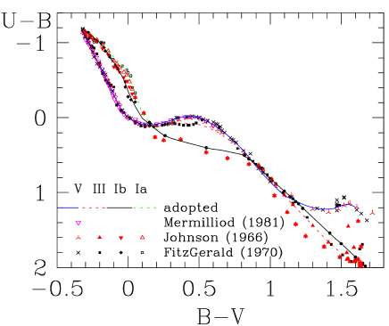
Fig. 4.—: The ($U-B,~{}B-V$) color-color diagram. Solid and dashed lines represent the adopted relations. The meaning of the symbols is explained in the figure.

The interstellar reddening can be determined from the two-color diagrams (hereinafter TCDs) using the difference in the color excess ratios between colors. Although several TCDs are used in the reddening estimate, the ($U-B,~{}B-V$) TCD is the most popular and a well-established one. To derive the reddening $E(B-V)$, we should adopt two relations: (1) the intrinsic color relation for the MS (or ZAMS) stars in the ($U-B,~{}B-V$) diagram , and (2) the slope of the reddening vector in the TCD.

The intrinsic color relation in the ($U-B,~{}B-V$) diagram was investigated by several researchers after the introduction of the $UBV$ photometric system. Among them, the relations derived by Johnson (1966), Mermilliod (1981), Schmidt-Kaler (1982), and FitzGerald (1970) are most frequently used. We compared their relations in Figure 4 and presented the adopted relation in Table 1. While Johnson (1966) and FitzGerald (1970) derived and presented the relations for all the luminosity classes, Mermilliod (1981) presented the relation only for MS stars derived from a comparative study of several well-observed open clusters. For early-type stars we adopt mainly the relation presented by Mermilliod (1981) for MS stars and the one of Johnson (1966) for the other LCs. For late-type stars we adopt the data by FitzGerald (1970) and smoothed the relations.

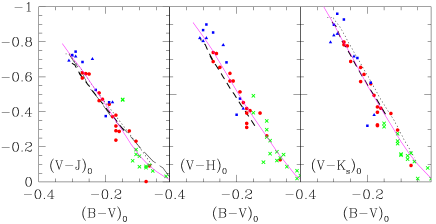
Fig. 5.—: The intrinsic color relation between ($B-V$)₀ and 2MASS colors. Red dot, green cross, blue square and blue triangle represent respectively, the star in NGC 2362, the Pleiades, NGC 2264, and the ONC, while the thick dashed, thin long dashed, dotted, and solid lines denote the synthetic color from Tlusty non-LTE model atmosphere, Johnson (1966)’s relation for supergiants, Johnson (1966)’s relation for MS, and the adopted relation, respectively.

The color excess in other colors, for e.g. $E(V-I)$, $E(V-J)$, $E(V-H)$, or $E(V-K_{s})$, cannot be easily determined from the TCD. The color excess can be determined from the intrinsic color relations between color and ($B-V$)₀. In addition, as the near- and mid-infrared color excess ratios are very sensitive to the reddening law (Guetter & Vrba 1989), i.e. the total to selective extinction ratio $R_{V}\equiv A_{V}/E(B-V)$, we derived the intrinsic color relations between ($B-V$)₀ and ($V-\lambda$)₀ for the 2MASS pass bands (Skrutskie et al. 2006).

To derive those relations, we chose 2MASS data for the Pleiades, NGC 2362, NGC 2264, and the ONC. In addition, we also calculated the synthetic colors in 2MASS and Spitzer IRAC bands using the Tlusty non-LTE model atmosphere of O- and B-type stars (Lanz & Hubeny 2003, 2007) by one of the authors (MSB). As these clusters are relatively less reddened, the uncertainty due to the reddening correction can be minimized. We assumed $E(B-V)$ = 0.10 and 0.04 mag for NGC 2362 and the Pleiades, respectively. The $E(B-V)$ of individual stars is estimated and corrected for the stars in NGC 2264 and the ONC. In correcting for the color excess for each color, we used the relation between the color excess ratio and the value of $R_{V}$ of Guetter & Vrba (1989) for 2MASS colors. We present the intrinsic color relations in Figure 5 and Table 2.

Table 2. : Intrinsic color relations for 2MASS colors

$B-V$	$V-J$	$V-H$	$V-Ks$
-0.33	-0.79	-0.91	-1.00
-0.30	-0.71	-0.83	-0.90
-.275	-0.65	-0.76	-0.81
-0.25	-0.58	-0.68	-0.73
-.225	-0.51	-0.60	-0.64
-0.20	-0.44	-0.52	-0.55
-.175	-0.36	-0.44	-0.47
-0.15	-0.29	-0.37	-0.39
-.125	-.215	-0.30	-0.31
-0.10	-0.15	-0.23	-0.23
-.075	-0.10	-0.16	-0.16
-0.05	-0.06	-0.10	-0.10
-.025	-0.03	-0.04	-0.05
0.00	0.00	0.00	0.00

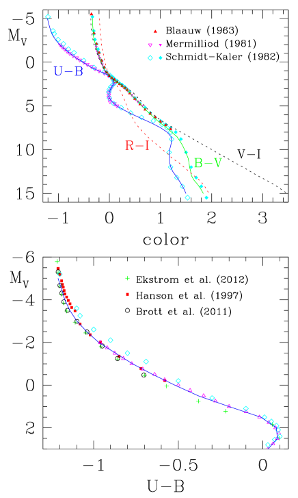
Fig. 6.—: Zero-Age Main Sequence relations. The solid and dashed lines represent the adopted ZAMS relations for the given color indices. Open circles, open diamonds and triangles represent the ZAMS relations by Mermilliod (1981), Schmidt-Kaler (1982), and Blaauw (1963), respectively.

4.2 Zero-Age Main-Sequence Relations

Table 3. : Zero-Age Main Sequence relations

$M_{V}$	$B-V$	$U-B$	$V-I$	$R-I$
-5.0	-0.33	-1.21	-0.36	-0.19
-4.5	-0.33	-1.19	-0.36	-0.19
-4.0	-.325	-1.17	-.355	-0.18
-3.5	-0.32	-1.15	-0.35	-0.18
-3.0	-0.31	-1.10	-0.33	-0.17
-2.5	-.295	-1.04	-0.32	-0.16
-2.0	-0.27	-0.97	-0.30	-0.15
-1.5	-.245	-0.87	-0.27	-0.14
-1.0	-0.22	-0.77	-0.24	-0.12
-0.5	-.185	-0.65	-.205	-.105
0.0	-.155	-0.52	-0.17	-.085
0.5	-0.12	-0.38	-0.13	-0.06
1.0	-.075	-0.20	-0.08	-0.04
1.5	-0.01	-0.01	-.015	-.005
2.0	.085	0.08	0.09	0.06
2.5	0.20	.085	0.23	0.13
3.0	0.31	0.03	.365	0.19
3.5	.395	-0.01	.465	.235
4.0	.475	-0.01	0.55	.275
4.5	0.56	0.05	0.63	0.31
5.0	0.64	0.15	0.69	0.34
5.5	0.72	0.29	0.77	0.37
6.0	0.81	0.47	0.86	0.42
6.5	0.90	0.65	0.97	0.47
7.0	1.01	0.84	1.10	0.51
7.5	1.12	1.00	1.25	0.58
8.0	1.22	1.13	1.40	0.66
8.5	1.32	1.21	1.56	.745
9.0	1.38	1.22	1.70	0.84
9.5	1.43	1.20	1.86	0.95
10.0	1.47	1.18	2.00	1.04
11.0	1.54	1.17	2.31	1.23
12.0	1.57	1.20	2.61	1.46
13.0	1.61	1.30	2.90	1.66
14.0	1.73	1.41	3.22	1.84
15.0	1.84	1.50	3.48	1.95

The ZAMS relation is the basic tool used to estimate the distance to open clusters. As noticed by Johnson & Hiltner (1956), the distance to an open cluster may have a large error if the effect of evolution during the MS phase is neglected. They introduced the standard main sequence for age “zero”. Sandage (1957) used the term “zero-age main sequence”. There are several standard clusters used in deriving the ZAMS relation. The primary cluster is the Hyades, which was the only cluster having a reliable distance at that time. The Pleiades is the second cluster which can provide the ZAMS relation up to A-type stars. Unfortunately there are no young open clusters within 1kpc from the Sun (apart for some unsuitable extremely young clusters), which makes it difficult to extend the relation to the upper MS. The young open clusters are, in general, highly reddened, show a differential reddening across the cluster, and have an anomalous reddening law in many cases. In addition, the metallicity of stars in the Perseus arm is known to be lower than that of the stars in the Solar neighborhood. The ZAMS relation of Schmidt-Kaler (1982) is nearly identical to that of Blaauw (1963) which is very similar to that of Johnson & Hiltner (1956) or Sandage (1957). Mermilliod (1981) published a new ZAMS relation from the analysis of photometric data for many open clusters. His ZAMS relation is slightly fainter than the others (Blaauw 1963; Schmidt-Kaler 1982).

Sung & Bessell (1999) presented the ZAMS relation in $V-I$ color which is less sensitive to the metallicity difference. We adopt the ZAMS relations used in the data analysis. The upper part of the ZAMS is taken from the reddening corrected color-magnitude diagrams (CMDs) of the young open clusters in the $\eta$ Carina nebula (Hur et al. 2012) and NGC 6611. By the definition of “zero” age for single stars, we took the lower ridge line of the MS band as the ZAMS. For B- to G-type stars, we adopt the ZAMS relation of Mermilliod (1981). For faint stars we adopted the relation of Schmidt-Kaler (1982). The ZAMS relations for $V-I$ and $R-I$ are derived using the intrinsic color relations in Table 1.

Table 4. : Spectral type-$M_{V}$ relation

Sp	V	III	II	Ib	Iab	Ia
O3	-5.45	-5.90	-5.95	-6.05	-6.25	-6.45
O4	-5.35	-5.85	-5.95	-6.05	-6.35	-6.60
O5	-5.25	-5.80	-5.90	-6.05	-6.40	-6.75
O6	-5.10	-5.70	-5.85	-6.05	-6.45	-6.85
O7	-4.90	-5.55	-5.80	-6.05	-6.45	-6.95
O8	-4.70	-5.35	-5.70	-6.00	-6.50	-7.00
O9	-4.40	-5.10	-5.55	-6.00	-6.50	-7.00
B0	-3.85	-4.70	-5.35	-5.95	-6.50	-7.05
B1	-3.20	-4.20	-5.20	-5.90	-6.50	-7.05
B2	-2.50	-3.60	-5.00	-5.85	-6.50	-7.05
B3	-1.70	-3.00	-4.80	-5.80	-6.50	-7.05
B4	-1.25	-2.55	-4.60	-5.75	-6.50	-7.05
B5	-1.00	-2.15	-4.40	-5.70	-6.50	-7.05
B6	-0.70	-1.85	-4.20	-5.65	-6.50	-7.05
B7	-0.40	-1.50	-3.95	-5.55	-6.50	-7.07
B8	-0.15	-1.20	-3.65	-5.50	-6.50	-7.10
B9	0.30	-0.90	-3.40	-5.40	-6.55	-7.15
A0	0.65	-0.70	-3.20	-5.30	-6.55	-7.20
A2	1.30	-0.40	-2.90	-5.20	-6.65	-7.40
A5	1.95	0.05	-2.70	-5.00	-6.75	-7.80
A8	2.40	0.40	-2.50	-4.85	-6.75	-8.15
F0	2.70	0.60	-2.50	-4.75	-6.70	-8.30
F2	3.00	0.80	-2.50	-4.70	-6.60	-8.30
F5	3.50	1.00	-2.30	-4.60	-6.55	-8.20
F8	4.00	1.00	-2.30	-4.55	-6.45	-8.00
G0	4.40	0.95	-2.30	-4.50	-6.40	-8.00
G2	4.70	0.90	-2.30	-4.50	-6.30	-8.00
G5	5.10	0.85	-2.30	-4.50	-6.20	-7.95
G8	5.50	0.75	-2.30	-4.45	-6.15	-7.85
K0	5.90	0.60	-2.30	-4.40	-6.10	-7.75
K2	6.30	0.30	-2.30	-4.40	-6.00	-7.70
K5	7.30	-0.10	-2.30	-4.40	-5.90	-7.50
M0	8.80	-0.40	-2.40	-4.60	-5.70	-7.10
M1	9.40	-0.45	-2.40	-4.65	-5.65	-7.00
M2	10.1	-0.45	-2.40	-4.75	-5.60	-6.95
M3	10.7	-0.50	-2.45	-4.80	-5.60	-6.90

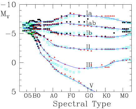
Fig. 7.—: Spectral type - M_V relation. Solid lines represent the adopted relations. Triangles, squares, dots, and open circles represent the relations by Blaauw (1963), Schmidt-Kaler (1982), Humphreys & McElroy (1984), and Conti et al. (1983), respectively.

The adopted ZAMS relations for several colors are presented in Figure 6. The ZAMS relations by Blaauw (1963), Mermilliod (1981), and Schmidt-Kaler (1982) are compared in the figure. In the lower panel, the ZAMS relation of the upper MS band is compared with those of Hanson et al. (1997), Brott et al. (2011), and Ekström et al. (2012) which are transformed using the Sp - color relations of Figure 12. For Brott et al. (2011), we took 10 models with the Milky Way abundance and nearly the same initial surface velocity for a given mass as those in Table 2 of Ekström et al. (2012). The ZAMS of Hanson et al. (1997) is slightly brighter than the adopted ZAMS, while that of Brott et al. (2011) and Ekström et al. (2012) is slightly fainter.

4.3 Spectral Type - M_V Relation

One may determine $R_{V}$ from the [$V-M_{V}$, $E(B-V)$] diagram. The absolute magnitude of a star can be determined from the ZAMS relation or from the Sp - $M_{V}$ relation for a given LC. In addition, one has to decide the membership of rare evolved stars in open clusters (see Lim et al. (2013) for example). For these reasons we have to adopt the Sp - $M_{V}$ relation. The usefulness of this relation is very limited because of the uncertainty in the LC. For O-type stars or evolved supergiant stars the scatter of $M_{V}$ is very large for a given Sp and LC because of their rarity and intrinsic variety of their characteristics.

Although there are several uncertainties, we adopt the Sp - $M_{V}$ relation in order to have a constraint for the membership of supergiant stars and early-type stars. We present the adopted Sp - $M_{V}$ relation in Figure 7 and in Table 4. The results from Blaauw (1963), Schmidt-Kaler (1982), Conti et al. (1983), and Humphreys & McElroy (1984) are compared in the figure. The $M_{V}$ value of A – F giants of Schmidt-Kaler (1982) is somewhat fainter than the values of Blaauw (1963), probably because of the uncertainty of LC or the inclusion of subgiants, or both. The $M_{V}$ of Humphreys & McElroy (1984) is slightly brighter for M-type supergiants (LC: Ib). We mainly adopt the Sp - $M_{V}$ relation of Blaauw (1963) for late-type stars.

4.4 Spectral Type - Temperature Relations

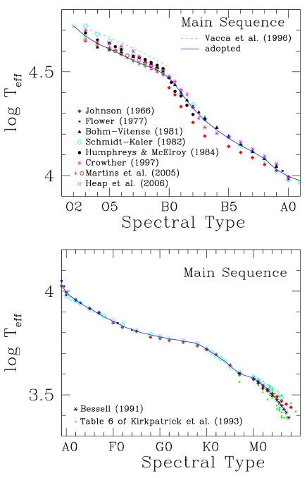
Fig. 8.—: Spectral type-effective temperature relation for MS stars. Solid lines represent the adopted relations.

One important aim of the SOS is to test observationally the stellar evolution theory. There are two observational tests - one is to compare observations with theoretical isochrones in the observational CMDs, the other is to compare the Hertzsprung-Russell diagrams (HRDs). In the first case, we have to use synthetic colors from model atmospheres, such as Bessell et al. (1998). For the second case, we need to transform observational quantities into physical parameters, such as T_eff and BC. Another important aim of the SOS is to address whether the stellar IMF is universal or not. To derive the IMF of an open cluster, one can directly determine the mass of the star in the HRD or rely on the mass-luminosity relation from the theoretical isochrones. As many young open clusters show a non-negligible spread in stellar age, the use of theoretical mass-luminosity relations may be limited to the intermediate-age or old open clusters. To construct the HRD of an open cluster, we should adopt the relations between Sp and T_eff, and between T_eff and BC. In this section, we describe the relation between Sp and T_eff for a given LC.

4.4.1 Main Sequence Stars

The color - T_eff relation has been studied by several authors. As shown in Figure 8, the T_eff scales are well consistent with each other for A – K stars, but shows a large scatter for hot or cool stars. For early-type stars, $B-V$ changes by only about 0.3 mag for O- and B-type stars (T_eff = 10,000 – 50,000 K) while $U-B$ changes by about 1.2 mag for the same T_eff range, but only shows a small change for O-type stars (Massey 1985). Therefore, although there is about 1 subclass uncertainty in spectral classification for O-type stars, Sp is the most important indicator of T_eff for them. We first derive the Sp - T_eff relation for MS stars. T_eff for a given O-type is generally lower for recent determinations than for older. For example, the T_eff scale of Crowther (1997) of O-type stars is slightly lower than that of Vacca et al. (1996), but higher than that of Martins et al. (2005) or Heap et al. (2006). We adopt the recent T_eff scale of Martins et al. (2005) (their observational T_eff scale) and that of Heap et al. (2006) for O-type stars.

The T_eff scales of B-type stars, especially for early B-type stars show a large scatter. The relation of Johnson (1966) gives the lowest T_eff, while others indicate a slightly higher T_eff. In addition, there is a large change in T_eff for early B-type stars. Unfortunately, the T_eff scale of these stars did not attract recent studies. We adopt the mean value of all the determinations except for Johnson (1966) for B-type stars.

The T_eff scales of M-type stars also show a large scatter. The T_eff scale of Johnson (1966) or Schmidt-Kaler (1982) is slightly higher, and that of Bessell (1991) slightly lower. The T_eff of Bessell (1991) is well-consistent with that of Kirkpartick et al. (1993). We adopt the T_eff scale of Bessell (1991) for M-type stars. For A – K-type stars, we take the mean value of Johnson (1966), Flower (1977), and Schmidt-Kaler (1982). The adopted T_eff scale for MS stars is shown with a solid line in Figure 8, and reported in Table 5.

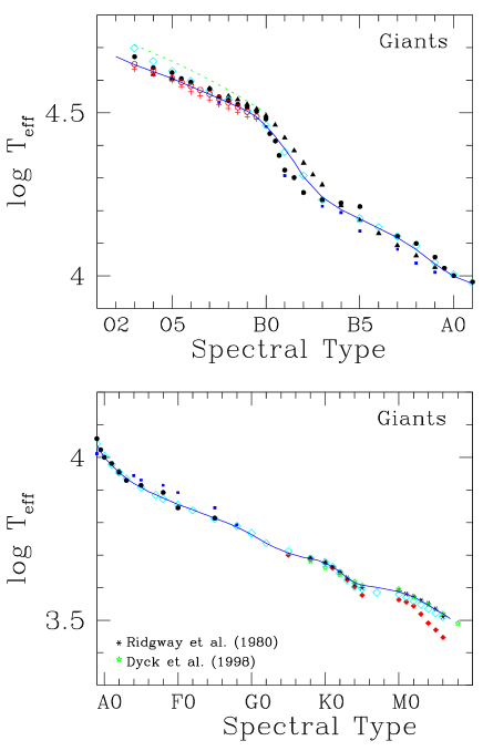
Fig. 9.—: Spectral-type-effective temperature relation for giant stars. Solid lines represent the adopted relations. Symbols are the same as in Figure 8 except for those in the lower panel.

4.4.2 Giant Stars

The T_eff scales of O-type giants show the same trend - lower T_eff for recent determinations. As for the case of MS stars, we choose the T_eff scale of Martins et al. (2005) for O-type stars. For B-type stars, the T_eff scale of Schmidt-Kaler (1982) is intermediate between Böhm-Vitense (1981) and Humphreys & McElroy (1984) or Flower (1977). We adopt the T_eff scale of Schmidt-Kaler (1982) for B-type stars.

For late-K and M-type stars, the T_eff scale of Johnson (1966) is lower than the others. We take the T_eff scale of Ridgway et al. (1980) for K and M-type stars. For A – K-type stars, Flower (1977) gives slightly higher T_eff. We mainly take Schmidt-Kaler (1982) for A – K-type stars. The adopted Sp - T_eff relation for giants is presented in Figure 9 and in Table 5.

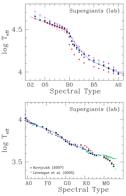
Fig. 10.—: Spectral type-effective temperature relation for supergiant stars. Solid lines represent the adopted relations. Symbols are the same as in Figure 8 except for those in the lower panel.

4.4.3 Supergiant Stars

The T_eff scale of early-type stars shows a large scatter as presented in Figure 10. The T_eff of B-type stars of Johnson (1966) is lower than the others. As is in the previous sections, we take the T_eff scale of Martins et al. (2005) for O-type stars, that of Crowther (1997) for early B stars, and that of Böhm-Vitense (1981) or Schmidt-Kaler (1982) for late B stars.

For A – G-type stars, the T_eff of Humphreys & McElroy (1984) is well consistent with that of Schmidt-Kaler (1982). We take the average of their relations. Recently Levesque et al. (2005) showed that there is a lower limit in the T_eff of M-type supergiants, and their T_eff scale of M-type is much higher than the others. We adopt the T_eff scale of Levesque et al. (2005) for M-type supergiants. The adopted Sp - T_eff relation is shown in Figure 10 and reported in Table 5.

4.5 Spectral Type - Color and Color - Temperature Relations

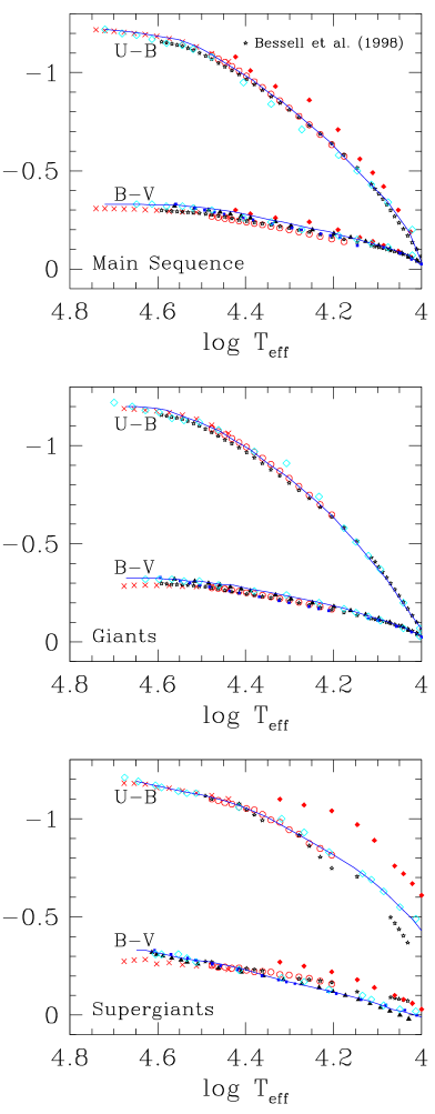
Fig. 11.—: Color - temperature relations for OB stars. Open circles, crosses, and star symbols represent the synthetic color from Tlusty O-type star models, Tlusty B-type star models, and Bessell et al. (1998) for MS stars (upper panel), for giant stars (middle panel), and for supergiant stars (LC = Iab, lower panel), respectively. The T_eff - $\log~{}g$ relation for a given LC is taken from Sung (1995). The other symbols are the same as those in Figure 8. Solid lines represent the adopted relations.

There are several studies on the Sp - color relations. Among them, FitzGerald (1970) analyzed extensive data in the $UBV$ photoelectric catalogue of Blanco et al. (1968). In general, these results are well-consistent with each other, as shown in Figure 12. However, in some cases, such as for B- and K-type stars where $U-B$ changes rapidly, it is not easy to take the intrinsic color for a given Sp. For such cases, we inevitably use the color-color relations adopted in Section 4.1. In addition, as the intrinsic color of early-type stars is still uncertain, we use the T_eff - color relations for early-type stars subsidarily (see Figure 11).

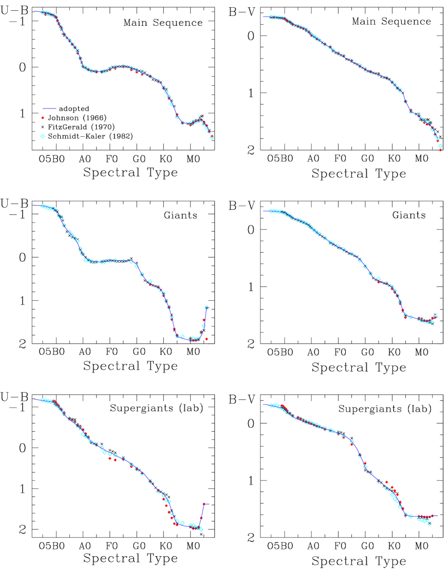
Fig. 12.—: Spectral type-color relations. Solid lines represent the adopted relations.

The $U-B$ colors from Tlusty models are in general well-consistent with the empirical relations, but the $B-V$ colors are slightly redder than the adopted relation by about 0.02 mag for MS and giants. The same is true for Bessell et al. (1998). In addition, the $U-B$ of Bessell et al. (1998) is slightly redder than the synthetic colors from Tlusty models for O- and early B-type stars. The color - T_eff relation of supergiant stars shows a large scatter. Nevertheless, the synthetic $U-B$ colors from Tlusty models are well-consistent with the $U-B$ versus T_eff relation of Schmidt-Kaler (1982). We adopt the $B-V$ versus T_eff relation using the color - color relation in Figure 4 for supergiant stars (Iab). The adopted relation is well-consistent with the empirical relation by Böhm-Vitense (1981) or Schmidt-Kaler (1982), but shows a different trend relative to the synthetic $B-V$ from the Tlusty models. The $U-B$ of Bessell et al. (1998) shows a large scatter due to the current limitation in models with $\log~{}g$ appropriate to supergiant stars (see Sung (1995) for the T_eff versus $\log~{}g$ relation). The adopted Sp - color relations are presented in Figure 12 and in Table 5.

4.6 Temperature - Bolometric Correction

Table 5. : Spectral type-T_eff-color relation

L.C.	V				III				Iab
Sp. Type	Teff	$B-V$	$U-B$	B.C.	Teff	$B-V$	$U-B$	B.C.	Teff	$B-V$	$U-B$	B.C.
O2	4.720	-0.33	-1.22	-4.52	4.672	-.325	-1.20	-4.22	4.648	-0.33	-1.19	-4.06
O3	4.672	-0.33	-1.21	-4.19	4.647	-.325	-1.20	-4.02	4.628	-0.33	-1.18	-3.90
O4	4.636	-0.33	-1.20	-3.94	4.626	-.325	-1.19	-3.88	4.607	-0.32	-1.17	-3.73
O5	4.610	-.325	-1.19	-3.77	4.605	-.325	-1.19	-3.72	4.585	-0.31	-1.16	-3.57
O6	4.583	-.325	-1.18	-3.58	4.580	-0.32	-1.18	-3.54	4.565	-0.30	-1.15	-3.43
O7	4.554	-.325	-1.17	-3.39	4.556	-0.32	-1.16	-3.39	4.544	-0.29	-1.14	-3.29
O8	4.531	-0.32	-1.15	-3.23	4.531	-0.31	-1.14	-3.21	4.519	-0.28	-1.13	-3.11
O9	4.508	-.315	-1.13	-3.03	4.505	-0.31	-1.12	-3.05	4.498	-.275	-1.12	-2.96
B0	4.470	-.305	-1.08	-2.84	4.459	-.295	-1.07	-2.73	4.445	-.255	-1.09	-2.66
B1	4.400	-.275	-0.98	-2.40	4.389	-0.27	-0.98	-2.41	4.353	-0.20	-1.01	-2.13
B2	4.325	-0.24	-0.87	-2.02	4.304	-.235	-0.84	-1.95	4.272	-.155	-0.91	-1.70
B3	4.265	-0.21	-0.75	-1.62	4.240	-.205	-0.72	-1.56	4.203	-0.12	-0.82	-1.31
B5	4.180	-0.17	-0.58	-1.22	4.175	-0.17	-0.57	-1.19	4.117	-0.07	-0.69	-0.87
B6	4.145	-0.15	-0.50	-1.02	4.146	-0.15	-0.50	-1.02	4.090	-0.05	-0.64	-0.73
B7	4.115	-0.13	-0.43	-0.85	4.117	-0.13	-0.42	-0.86	4.067	-0.03	-0.59	-0.60
B8	4.080	-0.11	-0.35	-0.66	4.080	-.105	-0.32	-0.66	4.044	-0.02	-0.54	-0.49
B9	4.028	-0.07	-0.19	-0.39	4.037	-0.07	-0.18	-0.44	4.021	-.005	-0.49	-0.38
A0	3.995	-0.01	-0.01	-0.24	3.998	-0.03	-0.06	-0.25	3.993	.015	-0.41	-0.26
A1	3.974	0.02	0.03	-0.15	3.976	0.01	0.01	-0.15	3.977	.035	-0.32	-0.20
A2	3.958	0.05	0.06	-0.08	3.954	0.05	0.06	-0.07	3.960	0.05	-0.23	-0.12
A3	3.942	0.08	0.08	-0.03	3.935	0.09	0.08	0.00	3.946	0.07	-0.15	-0.05
A5	3.915	0.15	0.10	0.00	3.907	0.15	0.10	0.05	3.928	0.10	-0.07	0.00
A6	3.902	0.18	0.10	0.01	3.895	0.19	0.11	0.06	3.920	0.11	-0.03	0.03
A7	3.889	0.21	0.09	0.02	3.885	0.22	0.11	0.06	3.910	.125	0.01	0.05
A8	3.877	0.25	0.08	0.02	3.875	0.25	0.10	0.06	3.902	0.14	0.05	0.07
F0	3.855	0.31	0.05	0.01	3.855	0.31	0.08	0.05	3.885	0.17	0.11	0.10
F1	3.843	0.34	0.02	0.01	3.847	0.33	0.07	0.04	3.875	0.19	0.14	0.11
F2	3.832	0.37	0.00	0.00	3.839	0.36	0.07	0.04	3.867	0.21	0.19	0.12
F3	3.822	0.40	-0.01	0.00	3.830	0.38	0.07	0.03	3.858	0.24	0.22	0.12
F5	3.806	0.45	-0.02	-0.01	3.813	0.43	0.08	0.02	3.836	0.32	0.28	0.11
F6	3.800	0.48	-0.01	-0.02	3.805	0.46	0.09	0.01	3.822	0.38	0.31	0.10
F7	3.794	0.50	0.00	-0.02	3.796	0.48	0.07	0.00	3.807	0.45	0.35	0.08
F8	3.789	0.53	0.02	-0.03	3.785	0.52	0.07	-0.01	3.790	0.55	0.40	0.05
G0	3.780	0.59	0.07	-0.04	3.763	0.64	0.17	-0.05	3.750	0.78	0.50	-0.05
G1	3.775	0.61	0.09	-0.04	3.750	0.70	0.30	-0.08	3.734	0.84	0.55	-0.09
G2	3.770	0.63	0.13	-0.05	3.737	0.77	0.41	-0.11	3.718	0.88	0.60	-0.16
G3	3.767	0.65	0.15	-0.06	3.725	0.85	0.49	-0.15	3.705	0.92	0.66	-0.21
G5	3.759	0.68	0.21	-0.07	3.706	0.90	0.62	-0.22	3.685	1.00	0.82	-0.32
G6	3.755	0.70	0.23	-0.08	3.700	0.92	0.65	-0.25	3.679	1.04	0.90	-0.35
G7	3.752	0.72	0.26	-0.09	3.693	0.94	0.67	-0.28	3.675	1.08	0.98	-0.37
G8	3.745	0.74	0.30	-0.10	3.689	0.96	0.70	-0.30	3.670	1.12	1.04	-0.40
K0	3.720	0.81	0.45	-0.18	3.675	1.01	0.87	-0.37	3.648	1.20	1.14	-0.54
K1	3.705	0.86	0.54	-0.24	3.664	1.08	1.02	-0.44	3.635	1.24	1.22	-0.65
K2	3.690	0.91	0.65	-0.32	3.648	1.16	1.16	-0.54	3.619	1.32	1.34	-0.80
K3	3.675	0.96	0.77	-0.41	3.630	1.26	1.36	-0.68	3.602	1.42	1.54	-0.98
K5	3.638	1.15	1.06	-0.65	3.607	1.50	1.83	-0.92	3.589	1.60	1.85	-1.14
M0	3.580	1.40	1.23	-1.18	3.588	1.57	1.92	-1.14	3.579	1.63	1.94	-1.27
M1	3.562	1.47	1.21	-1.39	3.580	1.59	1.92	-1.25	3.573	1.64	1.98	-1.35
M2	3.544	1.49	1.18	-1.64	3.572	1.60	1.92	-1.37	3.563	1.64	1.98	-1.53
M3	3.525	1.53	1.15	-2.02	3.559	1.60	1.90	-1.64	3.557	1.64	1.96	-1.64
M4	3.498	1.56	1.14	-2.55	3.547	1.60	1.81	-1.90	3.547	1.64	1.72	-1.82
M5	3.477	1.61	1.19	-3.05	3.533	1.57	1.65	-2.22	3.538	1.62	1.38	-2.05

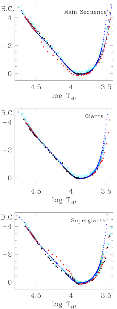
Fig. 13.—: Temperature-bolometric correction relations. Solid lines represent the adopted relations.

To construct the HRD, we need to correct for the amount of radiation emitted in the ultraviolet and in the infrared pass band. Johnson (1966) assumed BC = 0.00 for the Sun, and presented relatively smaller BC as shown in Figure 13. On the other hand, Schmidt-Kaler (1982) adopted BC = -0.19 for the Sun based on the Kurucz (1979) model atmospheres, and published relatively larger BC for all cases. Most astronomers now adopt $M_{bol}$ = 4.75 and BC = -0.07 for the Sun. Bessell et al. (1998) discussed this issue in detail.

As can be seen in Figure 13, BC is a function of T_eff for a given LC. Vacca et al. (1996) mentioned that BC for O-type stars is essentially a function of T_eff only, i.e. independent of surface gravity. Martins et al. (2005) presented a slightly smaller correction than that of Vacca et al. (1996), but BC is independent of surface gravity for O-type stars. Balona (1994) presented the relation between T_eff and BC for from O9 to G5 stars. Flower (1996) gave the same BC scale for MS and giant stars. Bessell et al. (1998) also calculated BC for a model atmosphere with various surface gravities, but there are non-negligible differences in BC among different LCs.

We assume that BC for O stars is independent of surface gravity, but that for B – M stars differs for different LCs. For M stars, we adopt the BC scale of Bessell (1991) for MS stars, Schmidt-Kaler (1982) for giant stars, and Levesque et al. (2005) for supergiant stars. For B – K stars, we adopt the BC scale of Bessell et al. (1998). The adopted BC scales are presented in Figure 13 and in Table 5.

5 DATA ANALYSIS TOOLS

5.1 Reddening Law

To determine the physical parameters of stars and clusters accurately, we should know the correct interstellar reddening. Many investigators determine the total extinction $A_{V}$ by assuming the total-to-selective extinction ratio $R_{V}$ to be 3.1. However, the interstellar reddening law $R_{V}$ is known to be different for different sightlines (Fitzpatrick & Massa 2009). In addition, many young open clusters are known to show an abnormal reddening law. Recently Sung et al. (2013, in preparation) confirmed the variation of the reddening law with Galactic longitude from an analysis of optical and 2MASS data for about 200 young open clusters.

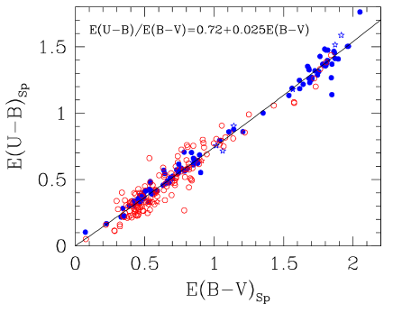
Fig. 14.—: Color excess ratio between $E(B-V)_{sp}$ and $E(U-B)_{sp}$ for O- and early B- (Sp $\leq$ B2.5) type stars in young open clusters. Dots and circles represent O- and B-type MS stars, respectively, while star symbols denote evolved stars.

Before determining the color excess ratio, we should determine the reddening $E(B-V)$ from the ($U-B,~{}B-V$) TCD. The slope of the reddening vector in the TCD is known to depend both on the amount of reddening and on the intrinsic color (see Golay (1974)). We determined $E(B-V)$ and $E(U-B)$ for about 255 OB-stars in the young open clusters (NGC 6530, $\eta$ Car, NGC 6611, NGC 6231, NGC 6823, IC 1805, Westerlund 2, NGC 2244, NGC 2264, and the ONC) using the relation between spectral type and intrinsic color (see Section 4.5), and this is shown in Figure 14. From the figure, we could not find any difference between O-type stars and B-type stars, which implies that the relation between $E(B-V)$ and $E(U-B)$ depends only on the amount of reddening. We adopt the excess ratio as follow;

$$E(U-B)/E(B-V)=0.72+0.025E(B-V).$$ (4)

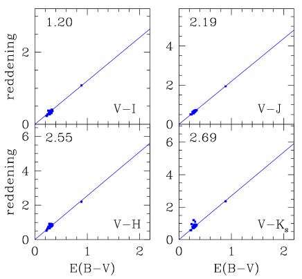
Fig. 15.—: Color excess ratios for NGC 6531. The color excess of each color is calculated using the relation between intrinsic colors (see Figure 5 and Table 2). The $UBVI$ CCD data are from Park et al. (2001). All four color excess ratios imply that $R_{V}$ = 2.96 $\pm$ 0.03 for NGC 6531.

Cardelli et al. (1989) showed that the total extinction $A_{\lambda}$ could be described as a simple function of $R_{V}$. If we assume their expression, the color excess can also be expressed as $E(U-B)/E(B-V)=0.859-0.045R_{V}$. If so, the ratio should be much smaller for young open clusters with an abnormal reddening law, e.g. the young open clusters in the $\eta$ Car nebula (Hur et al. 2012). We could not find any difference in color excess ratios among O-type stars in the $\eta$ Car nebula, and therefore we neglect the effect of $R_{V}$ on $E(U-B)/E(B-V)$.

Knowledge of the reddening law, especially the total-to-selective extinction ratio $R_{V}\equiv A_{V}/E(B-V)$, is very important in estimating the distance to the object. In general, $R_{V}$ can be determined from the color excess ratio (Guetter & Vrba 1989). We will determine the $R_{V}$ of target clusters using their relations,

$$R_{V}=2.45E(V-I)/E(B-V)$$ (5)

$$~{}=1.33E(V-J)/E(B-V)$$ (6)

$$~{}=1.17E(V-H)/E(B-V)$$ (7)

$$~{}=1.10E(V-K_{s})/E(B-V).$$ (8)

The reddening $E(B-V)$ of individual early-type stars is calculated from the ($U-B,~{}B-V$) TCD, and the color excess of each color is calculated using the relation between intrinsic colors described in Section 4.1. Figure 15 shows that the $R_{V}$ of NGC 6531 is 2.96 $\pm$ 0.03 from all the four colors.

5.2 Membership Selection Criteria

As open clusters are in the Galactic plane, we can expect many field interlopers in the foreground and background. Therefore, membership selection is crucial in the studies of a cluster. There are several different membership criteria for different clusters or for different age groups.

Proper motion studies are a classical membership criterion for cluster studies. To obtain reliable proper motions for the stars in the cluster field, a long baseline in time is very important. As old photographic plates have very low sensitivity, their limiting magnitude is about $V$ = 15 mag, which is far shallower than the limiting magnitude obtainable from a small telescope and from a modern CCD camera. The currently available CCD-based proper motion catalog from the US Naval Observatory, UCAC-3 (Zacharias et al. 2010) is in most cases useless for the membership selection of open clusters at 1 kpc or farther, because there is nearly no difference in proper motion between cluster members and field stars. The 10 $\mu as$ astrometric data from the Gaia astrometric satellite (Lindegren et al. 2007; Turon et al. 2012) will revolutionize the study of stellar astrophysics in the 2020s.

5.2.1 Early-Type Stars

Early-type members (Sp $\mathrel{\hbox{\hbox to0.0pt{\hbox{\lower 4.0pt\hbox{$\sim$}}\hss}\hbox{$<$}}}$ B5) in young or intermediate-age open clusters can be selected from the ($U-B$, $B-V$) TCD without any ambiguity. Unfortunately there is nearly no membership criterion for late-B or A – F-type stars in reddened clusters. In such cases we have to estimate the number of members in a statistical way, but it is impossible to assign a membership individually.

5.2.2 Young Open Clusters

Several membership criteria are used to select the low-mass PMS stars in young open clusters. Sung et al. (1997) introduced H$\alpha$ photometry as a membership criterion for low-mass PMS stars in the young open cluster NGC 2264, and successfully selected many PMS members in the T Tauri stage. H$\alpha$ photometry as a membership criterion is restricted to the extremely young open clusters with ages younger than about 5 Myr. Another method of membership selection in the optical pass bands is to study the variability because most young stars show variability due to mass accretion.

An important characteristic of young PMS stars is an IR excess emission from their circumstellar disks. Unfortunately most PMS stars do not show any appreciable emission in the near-IR pass bands. Therefore, the usefulness of near-IR $JHK$ photometry is very limited. An IR excess in the mid-IR pass bands, such as the Spitzer IRAC bands, is an important membership criterion for extreme young open clusters (Sung et al. 2009). The probability of membership selection from a mid-IR excess is very similar to that from H$\alpha$ photometry in the optical, but mid-IR excess is very useful for highly reddened embedded clusters.

While only classical T Tauri stars show very strong H$\alpha$ emission and an IR excess, both classical and weak-line T Tauri stars are very bright in X-rays. Therefore, X-ray emission is the most important membership criterion for low-mass PMS stars in young open clusters. Only a few PMS stars with edge-on disks do not show any appreciable emission or lack of emission (Sung et al. 2004). One weak point is that X-ray activity prolongs for a long time (Sung et al. 2008b). Hence, we need to pay attention to remove field interlopers with strong X-ray emission.

5.2.3 Intermediate-Age and Old Open Clusters

There is no reliable membership criterion for intermediate-age or old open clusters, except the CMD. For nearby clusters, Sung & Bessell (1999) devised a photometric membership criterion using the merit of multicolor photometry. Most intermediate-age or old open clusters do not show any appreciable amount of differential reddening across the cluster. In addition, the effect of reddening differs for different colors. The distance modulus from the ($V,~{}B-V$) CMD should be the same value [($V_{0}-M_{V})_{cl}$] as that from the ($V,~{}V-I$) CMD if the star is a member of the cluster. As photometric errors, binarity and other effects such as chromospheric activity (Sung et al. 2002) or metallicity difference (Sung & Bessell 1999) can also affect the ZAMS relation the criterion for membership selection should be relaxed - (i) the average value of the distance modulus should be in the range [($V_{0}-M_{V})_{cl}-0.75-2\sigma_{V_{0}-M_{V}}$] and [($V_{0}-M_{V})_{cl}+2\sigma_{V_{0}-M_{V}}$], and (ii) the difference in the distance moduli should be smaller than $2.5\sigma_{V_{0}-M_{V}}$.

For open clusters at 1 kpc or farther, we can expect many field interlopers with similar photometric characteristics. For such cases we should statistically estimate the number of field interlopers in the field region and subtract them (Kook et al. 2010).

5.3 Distance

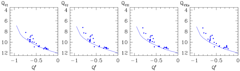
Fig. 16.—: The reddening-independent color-magnitude diagrams of NGC 6531 (Park et al. 2001). The distance modulus of 10.5 mag is applied for all CMDs. See the main text for details.

In general the distance to an open cluster is estimated using the ZAMS relation in the reddening-corrected CMDs. Before 1990, most observations were performed in $UBV$, and therefore the distance to an open cluster was estimated using the ZAMS relation in the ($M_{V},~{}B-V$) diagram. As the earlier CCDs were sensitive to longer wavelength, many $VRI$ or $BVRI$ CCD observations were performed in the 1990s. Although the flux measured at longer wavelength is less sensitive to the stellar parameters, the $RI$ pass bands have their own merits. They are less affected by the interstellar reddening and less sensitive to the difference in metallicity. The ZAMS relations in the optical pass bands, especially the $U$ and $B$ filters, can be affected by the difference in metallicity (Sung & Bessell 1999) as well as the chromospheric activity (Sung et al. 2002).

Sung & Bessell (2004) introduced a reddening-independent quantity Q${}_{VI}\equiv V-2.45(V-I)$ to estimate the distance to the starburst cluster NGC 3603. We introduce four reddening-independent quantities Q^′, Q_VJ, Q_VH, and Q${}_{VK_{s}}$.

$$Q^{\prime}\equiv(U-B)-0.72(B-V)-0.25E(B-V)^{2}$$ (9)

$$Q_{VJ}\equiv V-1.33(V-J)$$ (10)

$$Q_{VH}\equiv V-1.17(V-H)$$ (11)

$$Q_{VK_{s}}\equiv V-1.10(V-K_{s})$$ (12)

The parameter Q^′ is a modification of Johnson’s Q to take into account the effect of $E(B-V)$ on $E(U-B)/E(B-V)$, which is a non-negligible effect for highly reddened stars. The other three parameters are derived from the relation between $R_{V}$ and color excess ratios (see Section 5.1 or Guetter & Vrba (1989)). We determine the distance to an open cluster in the CMDs composed of Q^′ and Q_VI, Q_VJ, Q_VH, or Q${}_{VK_{s}}$ as shown in Figure 16.

The advantages of these quantities are (i) they are independent of interstellar reddening, (ii) homogeneous $JHK_{s}$ data are available from 2MASS, and (iii) they are less affected by differences in metallicity. In most cases we determine the distance to the cluster using the data for O and B-type stars, and so all the quantities are nearly free from metallicity differences. In addition, we can check for differences or errors in the photometric zero points from four CMDs, as shown in Figure 16. The photometric zero point of Park et al. (2001) is well consistent with those of 2MASS.

5.4 Age and Initial Mass Function

To determine the age and the IMF of an open cluster, we have to construct the HRD of the cluster using the calibrations adopted in Section 4. In addition, we need to adopt stellar evolution models to estimate the age and mass of a star. For a long time we have used the evolution models by the Geneva group (Schaller et al. 1992). Recently, Brott et al. (2011) and Ekström et al. (2012) published new stellar evolution models with stellar rotation. The results (age and the IMF) are very similar to each other (see for details Hur et al. (2012); Sung et al. (2013)).

As our survey is to observe a wide range of cluster ages, we will use the stellar evolution models by the Geneva group (Ekström et al. 2012) because their models cover a wide range of initial masses.

The importance of PMS stars in young open clusters is that their age and mass can be determined using PMS evolutionary models. The age distribution of a cluster represents the star formation history in the cluster. In addition, because many of our target clusters are relatively sparse, it is not easy to determine the age of a young open cluster with one or two O- or early B-type stars. On the other hand, as the low-mass PMS stars are relatively rich, it is easy to determine the age and the age spread of the cluster using low-mass PMS stars. We determine the age and mass of PMS stars in young open clusters using the PMS evolutionary models of Siess et al. (2000) since their models cover a relatively large mass range.

6 SUMMARY

Open clusters are the most important objects to test observationally stellar evolution theory which is a basic step toward an understanding of the Universe. We started the Sejong Open cluster Survey (SOS) dedicated to provide homogeneous photometry of a large number of open clusters in the Johnson-Cousins’ $UBVI$ system which is tightly matched to the SAAO standard system. The goals of this survey project are to study the various aspects of star formation and stellar evolution, and the structure, formation history and evolution of the Galactic disk.

In this paper, we also described the target selection criteria and the spatial distribution of targets based on the analysis of the open cluster database. In addition, we presented our strategy to achieve accurate and precise photometry.

To fulfill the goals of this project, we adopt and propose various calibrations and tools required for the analysis of photometric data. We described and compared various calibrations, and presented the adopted relations. These include the intrinsic color relations between various colors, the zero-age main sequence relations, the spectral type versus absolute magnitude relations, the spectral type versus effective temperature relations, the spectral type versus color relations, the color - temperature relations, and the temperature versus bolometric correction relations. In addition, we presented methods to determine the reddening law $R_{V}$ and the distance to the cluster.

ACKNOWLEDGMENTS H.S. acknowledges the support of the National Research Foundation of Korea (NRF) funded by the Korea Government (MEST) (Grant No.20120005318).

References

- Ann et al. (1999) Ann, H. B., Lee, M. G., Chun, M. Y., Kim, S.-L., Jeon, Y.-B., Park, B.-G., Yuk, I.-S., Sung, H., & Lee, S. H. 1999, BOAO Photometric Survey of Galactic Open Clusters. I. Berkeley 14 Collinder 74, Biurakan 9, and NGC 2355, JKAS, 32, 7
- Ann et al. (2002) Ann, H. B., Lee, S. H., Sung, H., Lee, M. G., Kim, S.-L., Chun, M.-Y., Jeon, Y. B., Park, B.-G., & Yuk, I, S. 2002, BOAO Photometric Survey of Galactic Open Clusters. II. Physical Parameters of 12 Open Clusters, AJ, 123, 905
- Balona (1994) Balona, L. A. 1994, Effective temperature, bolometric correction and mass calibration for O – F stars, MNRAS, 268, 119
- Bessell (1991) Bessell, M. S. 1991, The Late-M Dwarfs, AJ, 101, 662
- Bessell (1995) Bessell, M. S. 1995, UBVRI Systems: Resolving Different Versions, PASP, 107, 672
- Bessell et al. (1998) Bessell, M. S., Castelli, F., & Plez, B. 1998, Model atmospheres broad-band colors, bolometric corrections and temperature calibrations for O-M stars, A&A, 333, 231
- Bica et al. (2003) Bica, E., Dutra, C. M., Soares, J., & Barbuy, B. 2003, New infrared star clusters in the Northern and Equatorial Milky Way with 2MASS, A&A, 404, 223
- Blaauw (1963) Blaauw, A. 1963, in Basic Astronomical Data, Stars and Stellar Systems, Vol. 2, ed. by K. A. Strand (Chicago, Univ. of Chicago Press), p383
- Blanco et al. (1968) Blanco, V. M., Demers, S., Douglass, G. G., & FitzGerald, M. P. 1968, Photoelectric catalogue : magnitude and colors of stars in the , , , and , , systems, Pub. USNO, 21, 1
- Böhm-Vitense (1981) Böhm-Vitense, E. 1981, The Effective Temperature Scale, ARA&A, 19, 295
- Bragaglia & Tosi (2006) Bragaglia, A., & Tosi, M. 2006, The Bologna Open Cluster Chemical Evolution Project: Midterm Results from the Photometric Sample, AJ, 131, 1544
- Brott et al. (2011) Brott, I., de Mink, S. E., Cantiello, M., Langer, N., de Koter, A., Evans, C. J., Hunter, I., Trundle, C., & Vink, J. S. 2011, Rotating massive main-sequence stars. I. Grids of evolutionary models and isochrones, A&A, 530, 115
- Cardelli et al. (1989) Cardelli, J. A., Clayton, G. C., & Mathis, J. S. 1989, The relationship between infrared, optical, and ultraviolet extinction, ApJ, 345, 245
- Cheon et al. (2010) Cheon, S., Sung, H., & Bessell, M. S. 2010, No Open Cluster in the Ruprecht 93 Region, JKAS, 42, 115
- Conti et al. (1983) Conti, P. S., Garmany, C. D., de Loore, C., & Vanberen, D. 1983, The Evolution of Massive Stars: The Numbers and Distribution of O Stars and Wolf-Rayet Stars, ApJ, 274, 302
- Cousins & Caldwell (1998) Cousins, A. W. J. & Caldwell, J. A. R. 1998, Atmospheric extinction in the band, Observatory, 118, 85
- Crowther (1997) Crowther, P. A. 1997, The Effective Tepmeratures of Hot Stars. IAU Symp., 189, 137
- Dutra et al. (2003) Dutra, C. M., Bica, E., Soares, J., & Barbuy, B. 2003, New infrared star clusters in the southern Milky Way with 2MASS, A&A, 400, 533
- Ekström et al. (2012) Ekström, S. et al. 2012, Grids of stellar models with rotation. I. Models from 0.8 to 120 Msun at solar metallicity (Z = 0.014), A&A, 537, 146
- Fazio et al. (2004) Fazio, G. G., Hora, J. L., Allen, L. E. et al. 2004, The Infrared Array Camera (IRAC) for the Spitzer Space Telescope, ApJS, 154, 10
- FitzGerald (1970) FitzGerald, M. P. 1970, The Intrinsic olours of Stars and Two-Colour Reddening Lines, A&A, 4, 234
- Fitzpatrick & Massa (2009) Fitzpatrick, E. L., & Massa, D. 2009, An Analysis of the Shapes of Interstellar Extinction Curves. VI. The Near-IR Extinction Law, ApJ, 699, 1209
- Flower (1977) Flower, P. J. 1977, Transformations from Theoretical H-R Diagrams to C-M Diagrams: Effective Temperatures, Colors and Bolometric Corrections, A&A, 54, 31
- Flower (1996) Flower, P. J. 1996, Transformations from Theoretical Hertzsprung-Russell Diagrams to Color-Magnitude Diagrams: Effective Temperatures, B-V Colors, and Bolometric Corrections, ApJ, 469, 355
- Golay (1974) Golay, M. 1974, Introduction to Astronomical Photometry, (D.Reidel, Dordrecht-Holland), p.56
- Guetter & Vrba (1989) Guetter, H. H., & Vrba, F. J. 1989, Reddening and Polarimetric Studies toward IC 1805, AJ, 98, 611
- Heap et al. (2006) Heap, S. R., Lanz, T., & Hubeny, I. 2006, Fundamental Properties of O-Type Stars, ApJ, 638, 409
- Hanson et al. (1997) Hanson, M. M., Howarth, I. D., & Conti, P. S. 1997, The Young Stellar Objects of M17, ApJ, 489, 698
- Hoag et al. (1961) Hoag, A. A., Johnson, H. L., Iriarte, B., Mitchell, R. I., Hallam, K. L., & Sharpless, S. 1961, Photometry of Stars in Galactic Cluster Fields, Pub. USNO, 17, 347
- Humphreys & McElroy (1984) Humphreys, R. M., & McElroy, D. B. 1984, The Initial Mass Function for Massive Stars in the Galaxy and the Magellanic Clouds, ApJ, 284, 565
- Hur et al. (2012) Hur, H., Sung, H., & Bessell, M. S. 2012, Distance and the Initial Mass Function of Open Clusters in the eta Carina Nebula: Tr 14 and Tr 16, AJ, 143, 41
- Janes & Phelpse (1994) Janes, K. A., & Phelps, R. L. 1993, The Galactic system of old star clusters: The development of the Galactic disk, AJ, 108, 1773
- Johnson (1966) Johnson, H. L. 1966, Astronomical Measurements in the Infrared, ARA&A, 4, 193
- Johnson (1967) Johnson, H. L. 1967, The Law of Interstellar Extinction for Emission Nebulae Associated with O-Type tars, ApJ, 147, 912
- Johnson & Hiltner (1956) Johnson, H. L., & Hiltner, W. A. 1956, Observational Confirmation of a Theory of Stellar Evolution, ApJ, 123, 267
- Kalirai et al. (2001a) Kalirai, J. S., Richer, H. B., Fahlman, G. G., Cuillandre, J.-C., Ventura, P., D’Antona, F., Bertin, E., Marconi, G., & Durrell, P. R., 2001a, The CFHT Open Star Cluster Survey. I. Cluster Selection and Data Reduction, AJ, 122, 257
- Kalirai et al. (2001b) Kalirai, J. S., Richer, H. B., Fahlman, G. G., Cuillandre, J.-C., Ventura, P., D’Antona, F., Bertin, E., Marconi, G., & Durrell, P. R., 2001b, The CFHT Open Star Cluster Survey. II. Deep CCD Photometry of the Old Open Star Cluster NGC 6819, AJ, 122, 266
- Kalirai et al. (2001c) Kalirai, J. S., Ventura, P., Richer, H. B., Fahlman, G. G., Durrell, P. R., D’Antona, F., & Marconi, G., 2001c, The CFHT Open Star Cluster Survey. III. The White Dwarf Cooling Age of the Rich Open Star Cluster NGC 2099 (M37), AJ, 122, 3239
- Karachenko et al. (2005) Kharchenko, N. V., Piskunov, A. E., Röser, S., Schilbach, E., & Scholz, R.-D. 2005, 109 new Galactic open clusters, A&A, 440, 403
- Kilkenny et al. (1998) Kilkenny, D., van Wyk, F., Roberts, G., Marang, F., & Cooper, D. 1998, Supplementary southern standards for UBV(RI)c photometry, MNRAS, 294, 93
- Kim et al. (2003) Kim, S. C., & Sung, H. 2003, Physical Parameters of the Old Open Cluster Trumpler 5, JKAS, 36, 13
- Kirkpartick et al. (1993) Kirkpartick, J. D., Kelly, D. M., Rieke, G. H., Liebert, J., Allard, F., & Wehrse, R. 1993, M Dwarf Spectra from 0.6 to 1.5 Microns: A Spectral Sequence, Model Atmosphere Fitting, and the Temperature Scale, ApJ, 402, 643
- Kook et al. (2010) Kook, S.-H., Sung, H., & Bessell, M. S. 2010, CCD Photometry of the Open Clusters NGC 4609 and Hogg 15, JKAS, 42, 141
- Kurucz (1979) Kurucz, R. L. 1979, Model atmospheres for G, F, A, B, and O stars, ApJS, 40, 1
- Lada & Lada (2003) Lada, C., & Lada, E. 2003, Embedded Clusters in Molecular Clouds, ARA&A, 41, 57
- Landolt (1992) Landolt, A. U. 1992, Photometric Standard Stars in the Magnitude Range 11.5 16.0 around the Celestial Equator, AJ, 104, 340
- Lanz & Hubeny (2003) Lanz, T. & Hubeny, I. 2003, A Grid of Non-LTE Line-blanketed Model Atmospheres of O-Type Stars, ApJS, 146, 417
- Lanz & Hubeny (2007) Lanz, T. & Hubeny, I. 2007, A Grid of Non-LTE Line-blanketed Model Atmospheres of Early B-Type Stars, ApJS, 169, 83
- Levesque et al. (2005) Levesque, E. M., Massey, P., Olsen, K. A. G., Plez, B., Josselin, E., Meader, A., & Meynet, G. 2005, The Effective Temperature Scale of Galactic Red Supergiants: Cool, but Notas Cool as We Thought, ApJ, 628, 973
- Lim et al. (2013) Lim, B., Chun, M.-Y., Sung, H., Park, B.-G., Lee, J.-J., Sohn, S. T., Hur, H., & Bessell, M. S. 2013, The Starburst Cluster Westerlund 1: The Initial Mass Function and Mass Segregation, AJ, 145, 46
- Lim et al. (2009) Lim, B.-D., Sung, H., Bessell, M. S., Karimov, R., & Ibrahimov, M. 2009, CCD Photometry of Standard Stars at Maidanak Observatory in Uzbekistan: Transformation and Comparisons, JKAS, 41, 161
- Lim et al. (2008) Lim, B., Sung, H., Karimov, R., & Ibrahimov, M. 2008, Characteristics of the Fairchild 486 CCD at Maidanak Astronomical Observatory in Uzbekistan, Pub. of the Korean Ast. Sco., 23, 1
- Lim et al. (2011) Lim, B., Sung, H., Karimov, R., & Ibrahimov, M. 2011, Sejong Open Cluster Survey. I. NGC 2353, JKAS, 43, 39
- Lindegren et al. (2007) Lindegren, L., Babusiaux, C., Bailer-Jones, C. et al. 2007, The Gaia mission: science, organization and present status, IAU Symp., 248, 217
- Luhman (2012) Luhman, K. L. 2012, The Formation and Early Evolution of Low-Mass Stars and Brown Dwarfs, ARA&A, 50, 65
- Maciejewski & Niedzielski (2007) Maciejewski, G., & Niedzielski, A. 2007, CCD BV survey of 42 open clusters, A&A, 467, 1065
- Martins et al. (2005) Martins, F., Schaerer, D., & Hillier, D. J., 2005, A new calibration of stellar parameters of Galactic O stars, A&A, 436, 1049
- Massey (1985) Massey, P. 1985, Wolf-Rayet Stars in Nearby Galaxies: Tracers of the most Massive Stars, PASP, 97, 5
- Massey (2003) Massey, P. 2003, Massive Stars in the Local Group: Implications for Stellar Evolution and Star Formation, ARA&A, 41, 15
- Mathieu (2000) Mathieu, R. D. 2000, The WIYN Open Cluster Study, in Stellar Clusters and Associations: Convection, Rotation, and Dynamos, Proc. ASPC, Vol. 198, eds. R. Pallavicini, G. Micela, and S. Sciortino, (ASP, San Francisco), p517
- Menzies et al. (1989) Menzies, J. W., Cousins, A. CW. J., Banfield, R. M., & Laing, J. D. 1989, UBV(RI)C standard stars in the E- and F-regions and in the Magellanic Clouds-a revised catalogue, SAAO Circ., 13, 1
- Menzies et al. (1991) Menzies, J. W., Marang, F., Laing, J. D., Coulson, I. M., & Engelbrecht, C. A. 1991, UBV(RI)C photometry of equatorial standard stars-A direct comparison between the northern and southern systems, MNRAS, 248, 642
- Mermilliod (1981) Mermilliod, J.-C. 1981, Comparative Studies of Young Open Clusters III. Empirical Isochronous Curves and the Zero Age Main Sequence, A&A, 97, 235
- Mermilliod & Paunzen (2003) Mermilliod, J.-C., & Paunzen, E. 2003, Analysing the database for stars in open clusters I. General methods and description of the data, A&A, 410, 511
- Moffat & Vogt (1973a) Moffat, A. F. J. & Vogt, N. 1973a, Southern open stars clusters. III. UBV-H photometry of 28 clusters between Galactic longitudes 297∘ and 353∘, A&AS, 10, 135
- Moffat & Vogt (1973b) Moffat, A. F. J. & Vogt, N. 1973b, Photographic UBV photometry of ten open star clusters in a Galactic field at 1 = 135∘, A&AS, 11, 3
- Moffat & Vogt (1975a) Moffat, A. F. J. & Vogt, N. 1975a, Southern open star clusters IV. UBV-H photometry of 26 clusters from Monoceros to Vela, A&AS, 20, 85
- Moffat & Vogt (1975b) Moffat, A. F. J. & Vogt, N. 1975b, Southern open star clusters V. UBV-H photometry of 20 clusters in Carina, A&AS, 20, 125
- Moffat & Vogt (1975c) Moffat, A. F. J. & Vogt, N. 1975c, Southern open star clusters IV. UBV-H photometry of 18 clusters from Centaurus to Sagittarius, A&AS, 20, 155
- Park & Sung (2002) Park, B.-G., & Sung, H. 2002, & H Photometry of the Young Open Cluster NGC 2244, AJ, 123, 892
- Park et al. (2000) Park, B.-G., Sung, H., Bessell, M. S., & Kang, Y. H. 2000, The PMS Stars and Initial Mass Function of NGC 2264, AJ, 120, 894
- Park et al. (2001) Park, B.-G., Sung, H., & Kang, Y. H. 2001, The Galactic Open Cluster NGC 6531 (M21), JKAS, 34, 149
- Phelps & Janes (1993) Phelps, R. L., & Janes, K. A. 1993, Young open clusters as probes of the star-formation process. 2: Mass and luminosity functions of young open clusters, AJ, 106, 1870
- Piatti & Clariá (2001) Piatti, A. E., & Clariá, J. J. 2001, On the stellar content of the open clusters Melotte 105, Hogg 15, Pismis 21 and Ruprecht 140, A&A, 370, 931
- Porras et al. (2003) Porras, A., Christopher, M., Allen, L., Di Francesco, J., Megeath, S. T., Myers, P. C. 2003, A Catalog of Young Stellar Groups and Clusters within 1 Kiloparsec of the Sun, AJ, 126, 1916
- Ridgway et al. (1980) Ridgway, S. T., Joyce, R. R., White, N. M., & Wing, R. F. 1980, Effective Temperatures of Late-Type Stars: The Field Giants from K0 to M6, ApJ, 235, 126
- Sandage (1957) Sandage, A. 1957, Observational Approach to Evolution. II. A Computed Luminosity Function for K0 – K2 Stars from MV = +5 to MV = -4.5, ApJ, 125, 435
- Schaller et al. (1992) Schaller, G., Schaerer, D., Meynet, G., & Maeder, A. 1992, New grids of stellar models from 0.8 to 120 solar masses at Z = 0.020 and Z = 0.001, A&AS, 96, 269
- Schmidt-Kaler (1982) Schmidt-Kaler, K. 1982, in Landolt-Börnstein, Vol. 2b, p19, p31, p453
- Siess et al. (2000) Siess, L., Dufour, E., & Forestini, M. 2000, An internet server for pre-main sequence tracks of low- and intermediate-mass stars, A&A, 358, 593
- Skrutskie et al. (2006) Skrutskie, M. F., Cutri, R. M., Stiening, R. et al. 2006, The Two Micron All Sky Survey (2MASS), AJ, 131, 1163
- Stetson (2000) Stetson, P. B. 2000, Homogeneous Photometry for Star Clusters and Resolved Galaxies. II. Photometric Standard Stars, PASP, 112, 925
- Sung (1995) Sung, H. 1995, CCD Photometry of the Eight Young Open Clusters, PhD thesis, Seoul National University
- Sung & Bessell (1999) Sung, H., & Bessell, M.S. 1999, CCD Photometry of M35 (NGC 2168), MNRAS, 306, 361
- Sung & Bessell (2000) Sung, H., & Bessell, M.S. 2000, Standard Stars-CCD Photometry, Transformations and Comparisons, PASA, 17, 244
- Sung & Bessell (2004) Sung, H., & Bessell, M.S. 2004, The Initial Mass Function and Stellar Content of NGC 3603, AJ, 127, 1014
- Sung & Bessell (2010) Sung, H., & Bessell, M. S. 2010, The Initial Mass Function and Young Brown Dwarf Candidates of NGC 2264. IV. The Initial Mass Function and Star Formation History, AJ, 140, 2070
- Sung et al. (2004) Sung, H., Bessell, M. S., & Chun, M.-Y. 2004, The IMF and Young Brown Dwarf Candidates in NGC 2264. I. The IMF around S Monocerotis, AJ, 128, 1684
- Sung et al. (2008a) Sung, H., Bessell, M. S., Chun, M.-Y., Karimov, R., & Ibrahimov, M. 2008, The Initial Mass Function and Young Brown Dwarf Candidates of NGC 2264. III. Photometric Data, AJ, 135, 441
- Sung et al. (2002) Sung, H., Bessell, M. S., Lee, B.-W., & Lee, S.-G. 2002, The Open Cluster NGC 2516-I. Optical Photometry, AJ, 123, 290
- Sung et al. (1999) Sung, H., Bessell, M. S., Lee, H.-W., Kang, Y. H., & Lee, S.-W. 1999, CCD Photometry of M11 II. New Photometry and Surface Density Profiles, MNRAS, 310, 982
- Sung et al. (1997) Sung, H., Bessell, M.S., & Lee, S.-W. 1997, H Photometry of the Young Open Cluster NGC 2264, AJ, 114, 2644
- Sung et al. (1998) Sung, H., Bessell, M.S., & Lee, S.-W. 1998, and H Photometry of the Young Open Cluster NGC 6231, AJ, 115, 734
- Sung et al. (2000) Sung, H., Chun, M.-Y., & Bessell, M. S., 2000, & H Photometry of the Young Open Cluster NGC 6530, AJ, 120, 333
- Sung et al. (2008b) Sung, H., Bessell, M. S., & Sana, H. 2008, Coronal Temperature as an Age Indicator, JKAS, 41, 1
- Sung et al. (2013) Sung, H., Sana, H., & Bessell, M. S. 2013, The Initial Mass Function and the Surface ensity Profile of NGC 6231, AJ, 145, 37
- Sung et al. (2009) Sung, H., Stauffer, J., & Bessell, M. S. 2009, A Spitzer View of the Young Open Cluster NGC 2264, AJ, 138, 1116
- Turon et al. (2012) Turon, C., Luri, X., & Masana, E. 2012, Building the cosmic distance scale: from Hipparcos to Gaia, Astrophys Space Sci, 341, 15
- Vacca et al. (1996) Vacca, W. D., Garmany, C. D., & Shull, J. M. 1996, The Lyman-Continuum Fluxes and Stellar Parameters of O- and Early B-type stars, ApJ, 460, 914
- Vogt & Moffat (1972) Vogt, N., & Moffat, A. F. J. 1972, Southern open clusters I. UBV and H photometry of 15 clusters between Galactic longitudes 231∘ and 256∘, A&AS, 7, 133
- Vogt & Moffat (1973) Vogt, N., & Moffat, A. F. J. 1973, Southern open clusters II. UBV and H photometry of 11 clusters between Galactic longitudes 259∘ and 280∘, A&AS, 9, 97
- Zacharias et al. (2010) Zacharias, N., Finch, C., Girard, T. et al. 2010, The Third US Naval Observatory CCD Astrograph Catalog (UCAC3), AJ, 139, 2184