Joint Signal and Channel State Information
Compression for the Backhaul of Uplink
Network MIMO Systems

Abstract

In network MIMO cellular systems, subsets of base stations (BSs), or remote radio heads, are connected via backhaul links to central units (CUs) that perform joint encoding in the downlink and joint decoding in the uplink. Focusing on the uplink, an effective solution for the communication between BSs and the corresponding CU on the backhaul links is based on compressing and forwarding the baseband received signal from each BS. In the presence of ergodic fading, communicating the channel state information (CSI) from the BSs to the CU may require a sizable part of the backhaul capacity. In a prior work, this aspect was studied by assuming a Compress-Forward-Estimate (CFE) approach, whereby the BSs compress the training signal and CSI estimation takes place at the CU. In this work, instead, an Estimate-Compress-Forward (ECF) approach is investigated, whereby the BSs perform CSI estimation and forward a compressed version of the CSI to the CU. This choice is motivated by the information theoretic optimality of separate estimation and compression. Various ECF strategies are proposed that perform either separate or joint compression of estimated CSI and received signal. Moreover, the proposed strategies are combined with distributed source coding when considering multiple BSs. “Semi-coherent” strategies are also proposed that do not convey any CSI or training information on the backhaul links. Via numerical results, it is shown that a proper design of ECF strategies based on joint received signal and estimated CSI compression or of semi-coherent schemes leads to substantial performance gains compared to more conventional approaches based on non-coherent transmission or the CFE approach.

I Introduction

In network MIMO systems, multiple base stations (BSs), or remote radio heads, are connected via backhaul links to a central unit (CU). Under ideal BSs-to-CU connectivity conditions, the CU performs joint encoding in downlink and joint decoding in uplink on behalf of all the connected BSs (see [Gesbert10JSAC, SimeoneBookFnT, Marsch12VTMAG] and references therein). In the presence of practical limitations on the backhaul links, various strategies have been proposed for the communication between BSs and CU. Among these, one that appears to be favored due to its practicality and good theoretical performance is based on compress-and-forward [LightradioAL, Sanderovich09TIT, Tian09TIT, Xie13TIT]. Accordingly, focusing on the uplink, the BSs compress the received baseband signal and forward it to the CU. Network MIMO with compress-and-forward BSs is also known as cloud radio access (see, e.g., [IntelCor, LiuCOMMAG2011, ChinaMobile, FlanaganTI2011, Ericsson2012, HeathCOMMAG2011]).

Previous work on the design of backhaul compression strategies for the uplink has focused mostly on the problem of compressing the baseband received signal, and has implicitly assumed full channel state information (CSI) to be available at the CU [Sanderovich09TIT, Coso09TWC, Park13TVT, Zhou12arXiv]. This assumption comes with little loss of generality in quasi-static channels in which the coherence time/bandwidth of the channel is large enough. In this case, in fact, the CSI overhead on the backhaul can be amortized within the channel coherence time. Instead, in the presence of time-varying or frequency selective channels, CSI overhead can become significant. Under this assumption, it is hence important to properly design the transfer of CSI and data from the BSs to the CU.

The backhaul overhead due to CSI transfer between BSs and CU in the uplink was studied in [Kobayashi11TSP, Caire10ITA] by adapting the standard model of [Hassibi03TIT]. Accordingly, the transmission period is divided into coherence intervals of limited lengths, each of which is used for both training and data transmission. It is recalled that, in [Hassibi03TIT], this model was used to study a point-to-point MIMO system, and then the analysis was extended for downlink MIMO systems (with no backhaul constraints) in [Zheng02TIT, Kobayashi11TCOM]. Related work that concerns models in which BSs are connected to one another (see, e.g., [Simeone09TIT, Aktas08TWC]) and CSI is imperfect can be found in [Marsch09ICC, Marsch11TWC].

In [Kobayashi11TSP], an uplink system is studied in which the received baseband signals are first compressed by each BS and then transmitted over the backhaul to the CU. The latter performs channel estimation based on the training part of the compressed received signals and then carries out joint decoding. We refer to this approach as Compress-Forward-Estimate (CFE). In this work, we instead study an alternative approach that is motivated by the classical information-theoretic result concerning the separation of estimation and compression [Witsenhausen80TIT]. This result states that, when compressing a noisy observation, it is optimal to first estimate the signal of interest and then compress the estimate, rather than to let the estimation be performed at the decoder’s side. Following this insight, we propose various strategies that are based on an Estimate-Compress-Forward (ECF) approach: each BS first estimates the CSI and then compresses it for transmission to the CU. Specifically, the proposed strategies carry out separate or joint compression of the estimated CSI and the received signal in the data part of the block.

The main contributions in this paper are summarized as follows:

• Proposal and analysis of a class of ECF strategies for the separate or joint compression of the estimated CSI and of the received data signal;

• Proposal and analysis of a novel semi-coherent processing strategy that is based on the compression of the data signal after equalization at the BSs;

• Thorough performance comparison among the non-coherent transmission scheme, the CFE method [Kobayashi11TSP], and the proposed ECF and semi-coherent strategies via numerical results.

The rest of the paper is organized as follows. We first review the conventional schemes, namely the non-coherent approach and the CFE scheme in Section III. Then, we propose and analyze the ECF strategies in Section LABEL:Sec:SBC for the single-BS case and in Section LABEL:Sec:MBC for the more general scenario with multiple BSs. There, we combine the proposed ECF techniques with the distributed source coding strategies of [Coso09TWC]. Moreover, in Section LABEL:Sec:NCnSCP we propose “semi-coherent” schemes that do not convey any pilot information on the backhaul links. In Section LABEL:Sec:Numerical_Results, numerical results are presented. Concluding remarks are summarized in Section LABEL:Sec:Conclusion.

Notation: $E[\cdot]$, $\textrm{tr}(\cdot)$, and $\textrm{vec}(\cdot)$ denote the expectation, trace, and vectorization (i.e., stacking of the columns) of the argument matrix. The Kronecker product is denoted by $\otimes$. We use the standard notation for mutual information and differential entropy [GamalBook]. We reserve the superscript ${\bf{A}}^{T}$ for the transpose of ${\bf{A}}$, ${\bf{A}}^{\dagger}$ for the conjugate transpose of ${\bf{A}}$ and ${\bf{A}}^{-1}$ for the the pseudo-inverse ${\bf{A}}^{-1}=({\bf{A}}^{\dagger}{\bf{A}})^{-1}{\bf{A}}^{\dagger}$, which reduces to the usual inverse if the number of columns and rows are same. The matrices ${\bf{I}}_{i}$ and ${\bf{1}}_{i\times j}$ denote the $i\times i$ identity and the $i\times j$ all-one matrix, respectively. The covariance matrix ${\bf{R}}_{X}$ of the random vector $X$ is computed ${\bf{R}}_{X}=E[XX^{\dagger}]$, the cross covariance matrix ${\bf{R}}_{XY}$ of $X$ and $Y$ is ${\bf{R}}_{XY}=E[XY^{\dagger}]$, and ${\bf{R}}_{X|Y}$ denotes the conditional covariance matrix of $X$ conditioned on $Y$, i.e., ${\bf{R}}_{X|Y}={\bf{R}}_{X}-{\bf{R}}_{XY}{\bf{R}}_{Y}^{-1}{\bf{R}}_{XY}^{\dagger}$. The covariance matrix ${\bf{R}}_{Z}$ of a matrix ${\bf{Z}}$ is denoted by ${\bf{R}}_{Z}=E[\textrm{vec}({\bf{Z}})\textrm{vec}({\bf{Z}})^{\dagger}]$. For a subset $\mathcal{S}\subseteq\{1,\dots,n\}$, given matrices ${\bf{X}}_{1},\dots,{\bf{X}}_{n}$, we define the matrix ${\bf{X}}_{\mathcal{S}}$ by stacking the matrices ${\bf{X}}_{i}$ with $i\in\mathcal{S}$ vertically in ascending order, namely ${\bf{X}}_{\mathcal{S}}=\left[{\bf{X}}_{1}^{T},\dots,{\bf{X}}_{n}^{T}\right]^{T}$.

II System Model

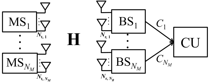
Figure 1: System model.

Consider the uplink of a cellular system consisting of $N_{M}$ MSs, $N_{B}$ BSs and a CU, as shown in Fig. 1. We denote the set of all MSs as $\mathcal{N}_{M}=\{1,\dots,N_{M}\}$ and of all BSs as $\mathcal{N}_{B}=\{1,\dots,N_{B}\}$. The MSs, the $i$-th of which has $N_{t,i}$ transmit antennas, communicate in the uplink to the BSs, where the $j$-th BS is equipped with $N_{r,j}$ receive antennas. Each $j$-th BS is connected to the CU via a backhaul link of capacity $C_{j}$. All rates, including $C_{j}$, are normalized to the bandwidth available on the uplink channel from MSs to BSs and are measured in bits/s/Hz. More precisely, we assume that $C_{j}TB$ bits can be transmitted on the backhaul by any $j$-th BS over an arbitrary number $B$ of coherence blocks. Note that each $j$-th BS can thus allocate its backhaul bits across different coherence blocks. This is akin to the standard long-term power constraints considered in a large part of the literature on fading channels (see, e.g., [Caire99TIT]). We define $N_{\min}=\min(N_{t},N_{r})$ and $N_{\max}=\max(N_{t},N_{r})$ where $N_{t}$ and $N_{r}$ are the number of total transmit antennas and total receive antennas, that is $N_{t}=\sum_{i=1}^{N_{M}}N_{t,i}$ and $N_{r}=\sum_{j=1}^{N_{B}}N_{r,j}$, respectively.

The channel coherence block, of length $T$ channel uses, is split it into a phase for channel training of length $T_{p}$ channel uses and a phase for data transmission of length $T_{d}$ channel uses, with

$$T_{p}+T_{d}=T,$$ (1)

as in [Kobayashi11TSP, Hassibi03TIT, Zheng02TIT, Kobayashi11TCOM]. The signal transmitted by the $i$-th MS is given by a $N_{t,i}\times T$ complex matrix ${\bf{X}}_{i}$, where each column corresponds to the signal transmitted by the $N_{t,i}$ antennas in a channel use. This signal is divided into the $N_{t,i}\times T_{p}$ pilot signal ${\bf{X}}_{p,i}$ and the $N_{t,i}\times T_{d}$ data signal ${\bf{X}}_{d,i}$. We assume that the transmit signal ${\bf{X}}_{i}$ has a total per-block power constraint $\frac{1}{T}\left\|{\bf{X}}_{i}\right\|^{2}=P_{i}$, and we define $\frac{1}{T_{p}}\left\|{\bf{X}}_{p,i}\right\|^{2}=P_{p,i}$ and $\frac{1}{T_{d}}\left\|{\bf{X}}_{d,i}\right\|^{2}=P_{d,i}$ as the powers used for training and data, respectively by the $i$-th MS. In terms of pilot and data signal powers, then, the power constraint becomes

$$\frac{T_{p}}{T}P_{p,i}+\frac{T_{d}}{T}P_{d,i}=P_{i}.$$ (2)

For simplicity, we assume equal transmit power allocation for each antenna of all MSs, and hence we have $P_{i}=P$, $P_{d,i}=P_{d}$ and $P_{p,i}=P_{p}$ for all $i\in\mathcal{N}_{M}$. We define ${\bf{X}}_{p}$ and ${\bf{X}}_{d}$ as the overall pilot signal and the data signal transmitted by all MSs, respectively, i.e., ${\bf{X}}_{p}=[{\bf{X}}_{p,1}^{T},\dots,{\bf{X}}_{p,N_{M}}^{T}]^{T}$ and ${\bf{X}}_{d}=[{\bf{X}}_{d,1}^{T},\dots,{\bf{X}}_{d,N_{M}}^{T}]^{T}$.

As in [Kobayashi11TSP, Hassibi03TIT], we assume that coding is performed across multiple channel coherence blocks. This implies that the ergodic capacity describes the system performance in terms of achievable sum-rate. Moreover, the training signal is ${\bf{X}}_{p}={\sqrt{\frac{P_{p}}{N_{t}}}}{\bf{S}}_{p}$ where ${\bf{S}}_{p}$ is a $N_{t}\times T_{p}$ matrix of i.i.d. $\mathcal{CN}(0,1)$ variables. This implies that an independently generated training sequence with power $P_{p}/N_{t}$ is transmitted from each transmitting antenna across all MSs. Similarly, during the data phase, the MSs transmit independent streams with power $P_{d}/N_{t}$ from its transmitting antennas using spatial multiplexing. As a result, we have ${\bf{X}}_{d}={\sqrt{\frac{P_{d}}{N_{t}}}}{\bf{S}}_{d}$ where ${\bf{S}}_{d}$ is a $N_{t}\times T_{d}$ matrix of i.i.d. $\mathcal{CN}(0,1)$ variables.

The $N_{r,j}\times T$ signal ${\bf{Y}}_{j}$ received by the $j$-th BS in a given coherence block, where each column corresponds to the signal received by the $N_{r,j}$ antennas in a channel use, can be split into the $N_{r,j}\times T_{p}$ received pilot signal ${\bf{Y}}_{p,j}$ and the $N_{r,j}\times T_{d}$ data signal ${\bf{Y}}_{d,j}$. The received signal at the $j$-th BS is then given by

$${\bf{Y}}_{p,j} = \sqrt{\frac{P_{p}}{N_{t}}}{\bf{H}}_{j}{\bf{S}}_{p}+{\bf{Z}}_{p,j}$$ (3a)

$$\textrm{and}\,\,\,\,{\bf{Y}}_{d,j} = \sqrt{\frac{P_{d}}{N_{t}}}{\bf{H}}_{j}{\bf{S}}_{d}+{\bf{Z}}_{d,j},$$ (3b)

where ${\bf{Z}}_{p,j}$ and ${\bf{Z}}_{d,j}$ are respectively the $N_{r,j}\times T_{p}$ and $N_{r,j}\times T_{d}$ matrices of independent and identically distributed (i.i.d.) complex Gaussian noise variables with zero-mean and unit variance, i.e, $\mathcal{CN}(0,1)$. The $N_{r,j}\times N_{t}$ channel matrix ${\bf{H}}_{j}$ collects all the $N_{r,j}\times N_{t,i}$ channel matrix ${\bf{H}}_{ji}$ from the $i$-th MS to the $j$-th BS as ${\bf{H}}_{j}=[{\bf{H}}_{j1},\dots,{\bf{H}}_{jN_{M}}]$.

The channel matrix ${\bf{H}}_{ji}$ is modeled as Rician fading with the line-of-sight (LOS) component $\bar{\bf{H}}_{ji}$, which is deterministic, and the scattered component ${\bf{H}}_{w,ji}$ with i.i.d. $\mathcal{CN}(0,1)$ entries. Overall, the channel matrix ${\bf{H}}_{ji}$ between the $j$-th BS and the $i$-th MS is represented as

$${\bf{H}}_{ji}=\sqrt{\alpha}_{ji}\left(\sqrt{\frac{K}{K+1}}\bar{\bf{H}}_{ji}+\sqrt{\frac{1}{K+1}}{\bf{H}}_{w,ji}\right),$$ (4)

where the Rician factor $K$ defines the power ratio of the LOS component and the scattered component, and the parameter $\alpha_{ji}$ represents the power gain between the $j$-th BS and the $i$-th MS. The channel matrix ${\bf{H}}_{j}$ is assumed to be constant during each channel coherence block and to change according to an ergodic process from block to block.

III Preliminaries

In this section, we discuss two reference schemes. The first is a non-coherent strategy, whereby the MSs do not transmit any pilot signal (i.e., $T_{p}=0$), each $j$-th BS compresses its received data signal (3b) for transmission on the backhaul, and the CU performs non-coherent decoding [Marzetta99TIT]. The second approach is the CFE strategy first studied in [Kobayashi11TSP], whereby each $j$-th BS compresses and transmits also its received pilot signals (3a); the CU estimates the CSI based on the compressed pilot signals received on the backhaul links; and the estimated CSI is then used by the CU to perform coherent decoding. To simplify the presentation, in this section, we assume a single BS, i.e., $N_{B}=1$, and hence drop the BS index $j$. Additionally, in non-coherent processing, we assume a single MS and drop the MS index $i$.

III-A Non-Coherent Processing

With non-coherent processing, the MS transmits the data signals ${\bf{X}}_{d}$ during the entire channel coherence time $T$ (i.e., $T_{p}=0$). The BS compresses the vector of received signals ${\bf{Y}}_{d}$ (3b) across all coherence times in the coding block and sends it to the CU on the backhaul link. Accordingly, the compressed received signals $\widehat{\bf{Y}}_{d}$ available at the CU can be written as

$$\widehat{\bf{Y}}_{d}={\bf{Y}}_{d}+{\bf{Q}}_{d},$$ (5)

where ${\bf{Q}}_{d}$ is independent of ${\bf{Y}}_{d}$ and represents the quantization noise matrix, which is assumed for simplicity to have i.i.d. $\mathcal{CN}(0,\sigma_{d}^{2})$ entries.

Remark 1

It is noted that, in principle, the design of the quantizers could be adapted to the channel statistics. Here, and in most of the paper, we instead assume i.i.d. quantization noises. Beside simplifying the system design, this choice is known to be optimal in the high-resolution regime (see the discussion on reverse waterfilling in [CoverBook, Ch. 10]). Another advantage of independent compression noises is that, if the signals to be compressed are not too correlated, then close-to-optimal quantization can be obtained with a separate quantizer for each component. $\hskip 8.5359pt\blacksquare$

Using standard rate-distortion theoretic arguments, the quantization noise $\sigma_{d}^{2}$ depends on the backhaul capacity via the equation $I({\bf{Y}}_{d};\widehat{\bf{Y}}_{d})=C$, which leads to $\sigma_{d}^{2}=(1+P)/(2^{(C/N_{r})}-1)$ (see, e.g., [GamalBook, Ch. 3]). A lower bound on the capacity achievable with non-coherent decoding can be obtained by substituting the equivalent SNR $\rho=P/(1+\sigma^{2}_{d})$ in [Marzetta99TIT, Eq. (10)].

III-B Compress-Forward-Estimate (CFE)

With the CFE scheme, the BS compresses both its received pilot signal (3a) and its received data signal (3b), and forwards them to the CU on the backhaul link. The CU then estimates the CSI based on the received compressed pilot signals and performs coherent decoding.

III-B1 Training Phase

During the training phase, the vector of received training signals ${\bf{Y}}_{p}$ (3a) across all coherence times is compressed as

$$\widehat{\bf{Y}}_{p}={\bf{Y}}_{p}+{\bf{Q}}_{p},$$ (6)

where the compression noise matrix ${\bf{Q}}_{p}$ is assumed to have i.i.d. $\mathcal{CN}(0,\sigma_{p}^{2})$ entries (see Remark 1). Based on (6), the channel matrix ${\bf{H}}_{i}$ from $i$-th MS to the BS is estimated at the CU by the minimum mean square error (MMSE) method. Hence, it can be expressed as

$${\bf{H}}_{i}=\widehat{\bf{H}}_{i}+{\bf{E}}_{i},$$ (7)

where the estimated channel $\widehat{\bf{H}}_{i}$ is a complex Gaussian matrix with mean matrix $\sqrt{\frac{\alpha_{i}K}{K+1}}\bar{\bf{H}}_{i}$ and covariance matrix $\sigma_{\widehat{h}_{i}}^{2}{\bf{I}}_{N_{r}N_{t,i}}$, and the estimation error ${\bf{E}}_{i}$ has i.i.d. $\mathcal{CN}(0,\sigma_{e_{i}}^{2})$ entries. The variances of the estimated channel and the estimation error can be calculated as $\sigma_{\widehat{h}_{i}}^{2}=\frac{{\frac{\alpha_{i}}{K+1}}T_{p}P_{p}}{{T_{p}P_{p}+N_{t}(1+\sigma_{p}^{2})({K+1})}}$ and $\sigma_{e_{i}}^{2}=\frac{\alpha_{i}N_{t}(1+\sigma_{p}^{2})}{{T_{p}P_{p}+N_{t}(1+\sigma_{p}^{2})({K+1})}}$, respectively (see, e.g., [Hassibi03TIT, Bjornson10TSP]).

III-B2 Data Phase

The compressed data signal received at the CU in (5) can be written as the sum of a useful term $\widehat{\bf{H}}{\bf{X}}_{d}$ and of the equivalent noise ${\bf{N}}_{d}={\bf{E}}{\bf{X}}_{d}+{\bf{Z}}_{d}+{\bf{Q}}_{d}$, namely

$$\widehat{\bf{Y}}_{d}=\widehat{\bf{H}}{\bf{X}}_{d}+{\bf{N}}_{d},$$ (8)

where the equivalent noise ${\bf{N}}_{d}$ has zero-mean and covariance matrix

$${\bf{R}}_{N}=E[{\textrm{vec}}({\bf{N}}_{d}){\textrm{vec}}({\bf{N}}_{d})^{\dagger}]=\left(1+\sigma_{d}^{2}+\frac{P_{d}}{N_{t}}\sum_{i=1}^{N_{M}}N_{t,i}\sigma_{e_{i}}^{2}\right){\bf{I}}_{N_{r}T_{d}}.$$ (9)

III-B3 Ergodic Achievable Rate

The ergodic capacity is given by the mutual information $\frac{1}{T}I({\bf{X}}_{d};\widehat{\bf{Y}}_{d}|\widehat{\bf{H}})$ [bits/s/Hz] (see, e.g, [GamalBook, Ch. 3]), which is bounded in the next lemma.