Investigations of the torque anomaly in an annular sector.
I. Global calculations, scalar case

Abstract

In an attempt to understand a recently discovered torque anomaly in quantum field theory with boundaries, we calculate the Casimir energy and torque of a scalar field subject to Dirichlet boundary conditions on an annular sector defined by two coaxial cylinders intercut by two planes through the axis. In this model the particularly troublesome divergence at the cylinder axis does not appear, but new divergences associated with the curved boundaries are introduced. All the divergences associated with the volume, the surface area, the corners, and the curvature are regulated by point separation either in the direction of the axis of the cylinder or in the (Euclidean) time; the full divergence structure is isolated, and the remaining finite energy and torque are extracted. Formally, only the regulator based on axis splitting yields the expected balance between energy and torque. Because of the logarithmic curvature divergences, there is an ambiguity in the linear dependence of the energy on the wedge angle; if the terms constant and linear in this angle are removed by a process of renormalization, the expected torque-energy balance is preserved.

I Introduction

Recently, evidence was presented fulling12 that the expected relation between energy and torque may not be satisfied by quantum vacuum energy. This conclusion is hard to accept, since the energy–torque balance formally follows from the general underlying variational principle dowker13 . Specifically, Ref. fulling12 considers the vacuum expectation values of the energy-momentum tensor for a wedge, for both a conformally coupled scalar field, where the wedge surfaces are Dirichlet boundaries, and for electromagnetism, where the boundaries are perfect conductors. These expectation values were evaluated many years ago by Dowker and Kennedy for the scalar case Dowker:1978md and then more generally by Deutsch and Candelas deutsch . (See also Refs. brevik and saharian .) Those papers presented calculations of the local stress tensor in the wedge geometry; if the $\langle T^{00}\rangle$ component is integrated over the region inside the wedge, or if $\langle T_{\theta\theta}\rangle$ is integrated over one of the bounding planes of the wedge, divergences are encountered because of the singularity of the field at the axis of the wedge. In Ref. fulling12 integration is therefore extended over a finite range of radial distances from the apex, and then it is found that the torque is not equal to the negative derivative of the energy with respect to the opening angle of the wedge. Because the stress tensors of the confomally invariant fields are completely finite in the radial range concerned, this result might be considered quite different from the pressure anomaly found earlier Estrada:2012yn for orthogonal plane boundaries, which can be blamed on a physically faulty regularization prescription. However, to extract the finite stress tensor, regularization of divergent quantities is required, so an issue arises that must be explored further.

It was immediately objected that this calculation does not describe a complete and physically acceptable model system. If the inner radius is taken to zero, one encounters the divergences at the axis; by subtracting infinities one can prove any result imaginable. If the reflecting wedge walls are simply truncated at a finite radius, one has a pair of finite, nonintersecting planes, requiring a different, and much harder, calculation. Instead, one can insert reflecting cylindrical boundaries at the inner and outer radii, producing a truncated sector as in Fig. 1.

Figure 1: Two radial Dirichlet plates, forming a dihedral angle $\alpha$, intersecting two coaxial Dirichlet cylinders of radius $a$ and $b$, forming an annular region. If the plane ribbons between the cylinders are imagined as free to slide in the circumferential, $\theta$, direction, maintaining contact with the cylindrical walls, this constitutes an annular piston. In this paper we are considering the interior sector alone; the exterior results are obtained by the replacement $\alpha\to 2\pi-\alpha$.

(It transpires that the outer cylinder is not very important, because the expectation values of the stress tensor fall off rapidly with radius. One could take the outer radius to infinity, but in this paper we prefer to keep it finite so that all terms in the regularized total energy will be finite.) This model is the most promising to study. Unfortunately, it introduces new divergences associated with the curvature of the bounding cylinders. Worse, some of these divergences are logarithmic (or would be associated with a pole of the zeta function), thereby creating an inherent ambiguity in the finite parts. As we shall see, this ambiguity is intimately connected to the existence of a torque anomaly.

Dowker dowker13 has outlined how the seemingly paradoxical torque anomaly might be resolved by solving the annular sector model introduced in the previous paragraph. The energy density and torque density associated with boundary regions near the cylinders, at finite radii, may display a precisely compensating imbalance, so that the annular system is nonanomalous. If this imbalance does not approach zero as the inner radius shrinks, its effect will be incorrectly lost in the calculation for the full wedge, in which there is no separate contribution from the apex of the wedge per se.

In this paper we examine a Dirichlet wedge intersected with a pair of coaxial, circular Dirichlet cylinders, as shown in Fig. 1. Thus an “annular piston” is realized, in which boundary motion takes place only inside the finite region defined between the concentric cylinders. That region consists of two “annular sectors” separated by the radial planes. In this paper we consider the total energy and torque for the scalar field in an annular sector, leaving local and electromagnetic calculations for future papers. We find the expected relation between the formal, unregulated expression for the torque on the radial planes and that for the interior energy, both of which are formally divergent. These expressions may be regulated by a regulator which does not depend on the opening angle of the wedge, in which case we might expect that the divergent (as the regulator goes to zero) and finite parts obey the expected energy-momentum balance. However, this turns out to be not quite the case: First, if all terms are taken seriously, only a neutral regulator (point separation in a direction not involved in the components of the stress tensor involved, in this case $z$ or $r$, the latter being less desirable because there is a boundary in that direction) gives the expected balance between energy and torque; this is precisely as expected from Ref. Estrada:2012yn . However, because of the logarithmic curvature divergences, there is an ambiguity in the linear dependence on the wedge angle in both the divergent and finite parts of the energy; if this arbitrary linear dependence is removed by a process of “renormalization,” all divergences and anomalies disappear, and the physical torque is the negative derivative with respect to the wedge angle of the physical energy, in agreement with previous considerations of the annular piston Milton:2009bz .

II Torque and energy on wedge intersected by coxial cylinders

We compute the torque and energy for the annular sector defined in Fig. 1, starting from the canonical flat-space stress tensor for a massless scalar field,

$$T^{\mu\nu}=\partial^{\mu}\phi\partial^{\nu}\phi-\frac{1}{2}g^{\mu\nu}\partial_{\lambda}\phi\partial^{\lambda}\phi,$$ (1)

in terms of the metric

$$g_{\mu\nu}=\mbox{diag}(-1,1,\rho^{2},1).$$ (2)

Thus, the angular-angular part of the stress tensor is

$$T^{\theta}{}_{\theta}=\frac{1}{2}\left(\partial^{0}\phi\partial^{0}\phi-\partial_{\rho}\phi\partial_{\rho}\phi+\frac{1}{\rho^{2}}\partial_{\theta}\phi\partial_{\theta}\phi-\partial_{z}\phi\partial_{z}\phi\right).$$ (3)

Here we adopt cylindrical coordinates, with the $z$ axis along the cylinder axis. Now to get the quantum vacuum stress, we replace

$$\phi(x)\phi(x^{\prime})\to\langle\phi(x)\phi(x^{\prime})\rangle=\frac{1}{i}G(x,x^{\prime}),$$ (4)

in terms of the Feynman or causal Green’s function. For the geometry considered we can represent the Green’s function as

$$G(x,x^{\prime}) = \int\frac{d\omega}{2\pi}e^{-i\omega(t-t^{\prime})}\int\frac{dk_{z}}{2\pi}e^{ik_{z}(z-z^{\prime})}$$ (5)

$$\quad\times\sum_{\nu}\Theta_{\nu}(\theta)\Theta_{\nu}^{*}(\theta^{\prime})g_{\nu}(\rho,\rho^{\prime}).$$

Here the eigenfunctions in $\theta$ and the corresponding eigenvalues $\nu$ are given by

$$\left[-\frac{\partial^{2}}{\partial\theta^{2}}+v(\theta)\right]\Theta_{\nu}(\theta)=\nu^{2}\Theta_{\nu}(\theta),$$ (6)

where the potential $v(\theta)$ represents the plane ribbons, so $v(\theta)=0$ within the sector. From this, we can integrate over the wedge surface at $\theta=\alpha$ to compute the torque on the plane at $\theta=\alpha$ per unit length (in the $z$ direction),

$$\tau = \int_{0}^{\infty}d\rho\,\rho\langle T^{\theta}{}_{\theta}\rangle(\rho,\alpha)$$

$$= \int_{0}^{\infty}d\rho\,\rho\frac{1}{2i}\int\frac{d\omega}{2\pi}\int\frac{dk_{z}}{2\pi}\sum_{\nu}\frac{1}{\rho^{2}}$$

$$\times(\partial_{\theta}\partial_{\theta^{\prime}}+\nu^{2})\Theta_{\nu}(\theta)\Theta_{\nu}^{*}(\theta^{\prime})g_{\nu}(\rho,\rho^{\prime})\bigg{|}_{\theta^{\prime}=\theta=\alpha,\rho^{\prime}=\rho}.$$

Let us simplify the following discussion by considering Dirichlet wedge surfaces, where the eigenvalues are explicit:

$$\nu=mp,\quad p=\frac{\pi}{\alpha},$$ (8)

and the eigenfunctions are explicitly

$$\Theta_{\nu}(\theta)=\sqrt{\frac{2}{\alpha}}\sin mp\theta.$$ (9)

Then the torque due to the field fluctuations interior to the annular sector is

$$\tau=\frac{1}{2\pi\alpha}\sum_{m=1}^{\infty}(mp)^{2}\int_{0}^{\infty}d\kappa\,\kappa\int_{a}^{b}\frac{d\rho}{\rho}g_{mp}(\rho,\rho),$$ (10)

where we have made a Euclidean rotation, $\omega\to i\zeta$, and adopted polar coordinates with $\kappa=\sqrt{\zeta^{2}+k^{2}_{z}}$.

The reduced Green’s function in the interior of the annular sector, $\rho\in[a,b]$, is

$$g_{\nu}(\rho,\rho^{\prime}) = I_{\nu}(\kappa\rho_{<})K_{\nu}(\kappa\rho_{>})$$

$$\quad\mbox{}-I_{\nu}(\kappa\rho)I_{\nu}(\kappa\rho^{\prime})\frac{K_{\nu}(\kappa a)K_{\nu}(\kappa b)}{\Delta}$$

$$\quad\mbox{}-K_{\nu}(\kappa\rho)K_{\nu}(\kappa\rho^{\prime})\frac{I_{\nu}(\kappa a)I_{\nu}(\kappa b)}{\Delta}$$

$$\quad\mbox{}+[K_{\nu}(\kappa\rho)I_{\nu}(\kappa\rho^{\prime})+I_{\nu}(\kappa\rho)K_{\nu}(\kappa\rho^{\prime})]$$ (11)

$$\quad\quad\times\frac{I_{\nu}(\kappa a)K_{\nu}(\kappa b)}{\Delta},$$

where the denominator is

$$\Delta=\Delta_{\nu}(\kappa a,\kappa b)=I_{\nu}(\kappa b)K_{\nu}(\kappa a)-I_{\nu}(\kappa a)K_{\nu}(\kappa b).$$ (12)

Now in terms of $Z_{\nu}(z),\tilde{Z}_{\nu}(z)=I_{\nu}(z)$ or $e^{i\nu\pi}K_{\nu}(z)$, the radial integrals may be evaluated by the following indefinite integral prudnikov :

$$\int\frac{dz}{z}Z_{\nu}(z)\tilde{Z}_{\nu}(z)=-\frac{Z_{\nu}(z)\tilde{Z}_{\nu}(z)}{2\nu}$$ (13)

$$\!\!\!\!\!\!\!\mbox{}-\frac{z}{2\nu}\left(Z_{\nu-1}(z)\frac{\partial}{\partial\nu}\tilde{Z}_{\nu}(z)-Z_{\nu}(z)\frac{\partial}{\partial\nu}\tilde{Z}_{\nu-1}(z)\right).$$

Consequently, the result of the radial integral in Eq. (10) is found by straightforward algebra:

$$\int_{a}^{b}\frac{d\rho}{\rho}g_{\nu}(\rho,\rho)=\frac{1}{2\nu}\frac{\partial}{\partial\nu}\ln\Delta_{\nu}(\kappa a,\kappa b).$$ (14)

From this, using

$$\frac{\partial}{\partial\nu}=-\frac{\alpha}{\nu}\frac{\partial}{\partial\alpha},$$ (15)

we find

$$\tau=-\frac{\partial}{\partial\alpha}\frac{1}{4\pi}\sum_{m=1}^{\infty}\int_{0}^{\infty}d\kappa\,\kappa\ln\Delta_{\nu}(\kappa a,\kappa b).$$ (16)

This exhibits the expected relation between torque and energy,

$$\tau=-\frac{\partial}{\partial\alpha}\mathscr{E},$$ (17)

provided the energy per unit length is

$$\mathscr{E}=\frac{1}{4\pi}\sum_{m=1}^{\infty}\int_{0}^{\infty}d\kappa\,\kappa\ln\Delta_{\nu}(\kappa a,\kappa b).$$ (18)

In fact, it is easy to calculate the interior energy of the annular sector. This may be computed from the integrated energy density,

$$\langle T^{00}\rangle=\frac{1}{2i}[\partial^{0}\partial^{\prime 0}-(\partial^{0})^{2}]G(x,x^{\prime})\big{|}_{x^{\prime}=x},$$ (19)

which leads to the general formula miltonbook

$$E=\int(d\mathbf{r})\int_{-\infty}^{\infty}\frac{d\omega}{2\pi i}\,\omega^{2}\mathscr{G}(\mathbf{r,r};\omega),$$ (20)

in terms of the Fourier transform of the Green’s function

$$G(x,x^{\prime})=\int_{-\infty}^{\infty}\frac{d\omega}{2\pi}e^{-i\omega(t-t^{\prime})}\mathscr{G}(\mathbf{r,r};\omega).$$ (21)

Here this reads for the energy per unit length

$$\mathscr{E}=-\frac{1}{4\pi}\int_{0}^{\infty}d\kappa\,\kappa^{3}\int_{a}^{b}d\rho\,\rho\sum_{m=1}^{\infty}g_{\nu}(\rho,\rho^{\prime}).$$ (22)

The radial integrals are straightforwardly evaluated prudnikov . The result

$$\mathscr{E}=-\frac{1}{8\pi}\sum_{m=1}^{\infty}\int_{0}^{\infty}d\kappa\,\kappa^{2}\frac{\partial}{\partial\kappa}\ln\Delta_{\nu}(\kappa a,\kappa b)$$ (23)

is indeed the energy shown in Eq. (18), after integration by parts, at this point purely formal.

Thus, we see at a formal level there is the correct balance between energy and torque, Eq. (17). Of course, the expressions for the torque and the energy given here are divergent. However, we might expect that as long as these integrals are regulated in a way that does not refer to the wedge angle $\alpha$, the divergent and finite parts of the torque and the energy will satisfy the same balance. In Sec. IV we will investigate this by introducing a point-splitting cutoff.

III Conformal terms

The above used the canonical stress tensor for the scalar field. More generally, the stress tensor is

$$T^{\mu\nu}=\partial^{\mu}\phi\partial^{\nu}\phi-\frac{1}{2}g^{\mu\nu}\partial_{\lambda}\phi\partial^{\lambda}\phi-\xi(\partial^{\mu}\partial^{\nu}-g^{\mu\nu}\partial^{2})\phi^{2},$$ (24)

where $\xi$ is an arbitrary parameter, and the corresponding term is identically conserved. The value of $\xi$ that makes conformal invariance manifest, and that makes the ultraviolet behavior of the theory most regular, is, in three spatial dimensions, $\xi=\frac{1}{6}$ Callan:1970ze ; Milton:1972cc . For example, when $\xi=1/6$, the divergences in the energy density near a Dirichlet surface are reduced from $1/z^{4}$ to $1/z^{3}$, where $z$ is the distance from the surface Milton:2010qr . However, this ambiguity is irrelevant when computing global quantities such as the total energy or the total torque Milton:2010qr . The reason is the following: Let us denote the conformal term in the stress tensor as

$$\Delta T^{\mu\nu}=-\xi(\partial^{\mu}\partial^{\nu}-g^{\mu\nu}\partial^{2})\phi^{2}.$$ (25)

For the torque contribution we need

$$\Delta T^{\theta\theta}=-\xi\left((\partial^{0})^{2}-\partial_{z}^{2}-\frac{1}{\rho}\partial_{\rho}\rho\partial_{\rho}\right)\phi^{2},$$ (26)

which for Dirichlet boundaries vanishes on either plate, $\theta=0$ or $\theta=\alpha$. This continues to be true if we point split in a direction which respects the boundary conditions, that is, in the $z$ direction or the $t$ direction. For the energy contribution we have

$$\Delta T^{00}=-\xi\nabla^{2}\phi^{2},$$ (27)

which, when integrated over a region with Dirichlet boundaries, vanishes because

$$\int_{V}(d\mathbf{r})\nabla^{2}\phi^{2}=2\oint_{\partial V}d\bm{\sigma}\cdot\phi\bm{\nabla}\phi=0.$$ (28)

This again holds even with point splitting in a direction perpendicular to the normals of the boundaries, here in the $z$ or $t$ directions.

IV Point splitting

We now redo the calculation in Sec. II. In view of the discussion in Sec. III, we point split in the directions either of $t$ or $z$. After the Euclidean rotation, the torque per length is

$$\tau=\frac{1}{2}\int_{a}^{b}\frac{d\rho}{\rho}\int\frac{d\zeta\,dk}{(2\pi)^{2}}e^{i\zeta t_{E}}e^{ikZ}\frac{2}{\alpha}\sum_{m=1}^{\infty}(mp)^{2}g_{mp}(\rho,\rho),$$ (29)

in place of Eq. (10), where $t_{E}=i(t-t^{\prime})$ and $Z=z-z^{\prime}$ are point-split regulator parameters, which are to be taken to zero. Now let us write

$$\zeta = \kappa\cos\gamma,\quad k=\kappa\sin\gamma,$$ (30a)

$$t_{E} = \delta\cos\phi,\quad Z=\delta\sin\phi,$$ (30b)

where $\delta\to 0$ and $\phi$ is an arbitrary angle. When $\phi=0$ we are doing time splitting, while if $\phi=\pi/2$, we are splitting the points at which the product of fields are evaluated at slightly different values of $z$. Thus, the regulator exponent is

$$\zeta t_{E}+kZ=\kappa\delta\cos(\gamma-\phi).$$ (31)

The regulated torque is, in fact, independent of $\phi$, and in place of Eqs. (10) and (16) we have

$$\tau = \frac{1}{2\pi\alpha}\int_{a}^{b}\frac{d\rho}{\rho}\int_{0}^{\infty}d\kappa\,\kappa\,J_{0}(\kappa\delta)\sum_{m=1}^{\infty}(mp)^{2}g_{mp}(\rho,\rho)$$ (32)

$$= -\frac{\partial}{\partial\alpha}\frac{1}{4\pi}\int_{0}^{\infty}d\kappa\,\kappa\,J_{0}(\kappa\delta)\sum_{m=1}^{\infty}\ln\Delta_{\nu}(\kappa a,\kappa b).$$

Is this the negative derivative of the energy?

The expectation value of the energy density, given in Eq. (19), leads to the following expression for the energy per unit length, using the same point splitting as above, instead of Eq. (22):

$$\mathscr{E}=-\int_{0}^{\infty}\frac{d\kappa\,\kappa^{3}}{2\pi}f(\kappa\delta,\phi)\sum_{m=1}^{\infty}\int_{a}^{b}d\rho\,\rho\,g_{\nu}(\rho,\rho),$$ (33)

where the regulator function is

$$f(\kappa\delta,\phi) = \int_{0}^{2\pi}\frac{d\gamma}{2\pi}\cos^{2}\gamma\,e^{i\kappa\delta\cos(\gamma-\phi)}$$

$$= \left[\frac{1}{2}J_{0}(\kappa\delta)-\frac{1}{\kappa\delta}J_{1}(\kappa\delta)\right]\cos 2\phi+\frac{1}{2}J_{0}(\kappa\delta),$$

which equals 1/2 as $\delta\to 0$. As before, the radial integral is

$$\int_{a}^{b}d\rho\,\rho\,g_{\nu}(\rho,\rho)=\frac{1}{2\kappa}\frac{\partial}{\partial\kappa}\ln\Delta_{\nu}(\kappa a,\kappa b),$$ (35)

so if we integrate by parts, the energy/length is

$$\mathscr{E}=\frac{1}{4\pi}\int_{0}^{\infty}d\kappa\frac{\partial}{\partial\kappa}\left[\kappa^{2}f(\kappa\delta,\phi)\right]\sum_{m=1}^{\infty}\ln\Delta_{\nu}(\kappa a,\kappa b).$$ (36)

Is this the quantity appearing in Eq. (32)? This would seem to require that

$$\frac{\partial}{\partial\kappa}\left[\kappa^{2}f(\kappa\delta,\phi)\right]=\kappa J_{0}(\kappa\delta).$$ (37)

Indeed this is so for the $z$ regulator, $\phi=\pi/2$. But it is not so for time splitting, where

$$\frac{\partial}{\partial\kappa}\left[\kappa^{2}f(\kappa\delta,0)\right]=\kappa J_{0}(\kappa\delta)+\kappa^{2}\delta J_{0}^{\prime}(\kappa\delta).$$ (38)

We will now proceed to see how the divergent and finite parts of the energy behave as functions of $\delta$, $\phi$, and $\alpha$.

V Weyl Terms

V.1 Leading Divergences

Let us now extract the leading divergences, as the cutoff $\delta\to 0$, in the energy using the form (36) (before the suspect integration by parts),

$$\mathscr{E}=-\frac{1}{4\pi}\int_{0}^{\infty}d\kappa\,\kappa^{2}f(\kappa\delta,\phi)\sum_{m=1}^{\infty}\frac{\partial}{\partial\kappa}\ln\Delta_{\nu}(\kappa a,\kappa b).$$ (39)

To do so, we use the uniform asymptotic expansions (nist, , 10.41.ii) of the modified Bessel functions, applicable as $\nu\to\infty$:

$$I_{\nu}(\nu z) \sim \sqrt{\frac{t}{2\pi\nu}}e^{\nu\eta}\left(1+\sum_{k=1}^{\infty}\frac{u_{k}(t)}{\nu^{k}}\right),$$ (40a)

$$K_{\nu}(\nu z) \sim \sqrt{\frac{\pi t}{2\nu}}e^{-\nu\eta}\left(1+\sum_{k=1}^{\infty}\frac{(-1)^{k}u_{k}(t)}{\nu^{k}}\right),$$ (40b)

where $t=(1+z^{2})^{-1/2}$, $\eta(z)=1/t+\ln\frac{z}{1+1/t}$. It follows that

$$\frac{d\eta}{dz}=\frac{1}{zt}.$$ (41)

Here the $u_{k}(t)$ are polynomials in $t$ of degree $3k$. If we retain only the leading factor, we get, with $\nu z=\kappa b$,

$$\Delta_{\nu}(\nu za/b,\nu z)\sim\frac{\sqrt{t(z)t(za/b)}}{\nu}\sinh\nu[\eta(z)-\eta(za/b)],$$ (42)

where $\nu z=\kappa b$. Thus, the leading divergence is obtained from

$$\ln\Delta_{\nu}(\kappa a,\kappa b)\sim\nu[\eta(z)-\eta(za/b)],$$ (43)

which has derivative

$$\frac{\partial}{\partial\kappa}\ln\Delta_{\nu}\sim\frac{b}{z}\left[\sqrt{1+z^{2}}-\sqrt{1+(za/b)^{2}}\right].$$ (44)

For the $z$-point-splitting, $\phi=\pi/2$, we have the following expression for the most divergent contribution:

$$\mathscr{E}_{4}(\pi/2) = -\frac{1}{4\pi b\delta}\sum_{m=1}^{\infty}\nu^{2}\int_{0}^{\infty}dz\,J_{1}(\nu z\delta/b)$$ (45)

$$\quad\times\left[\sqrt{1+z^{2}}-\sqrt{1+(za/b)^{2}}\right].$$

Although not classically convergent, the $z$ integral has a well-defined meaning:

$$\int_{0}^{\infty}dz\,J_{1}(az)\sqrt{1+z^{2}}=\frac{1}{a}+\frac{1}{a^{2}}e^{-a},$$ (46)

and then, approximating the sum on $m$ by an integral:

$$\sum_{m=1}^{\infty}\to\frac{\alpha}{\pi}\int_{0}^{\infty}d\nu,$$ (47)

we immediately find

$$\mathscr{E}_{4}(\pi/2) \sim -\frac{1}{4\pi\delta^{3}}\frac{\alpha}{\pi}\int_{0}^{\infty}d\nu\left[be^{-\nu\delta/b}-ae^{-\nu\delta/a}\right]$$

$$= -\frac{\alpha}{4\pi^{2}\delta^{4}}(b^{2}-a^{2})=-\frac{A}{2\pi^{2}\delta^{4}}=\mathscr{E}^{(4)}(\pi/2),$$

which exhibits the expected quartic divergence as the cutoff $\delta$ tends to zero. Here the area of the annular region is $A=\alpha(b^{2}-a^{2})/2$.

If we use the time-splitting cutoff instead, so $\phi=0$, and the regulator function is

$$f(\kappa\delta,0)=J_{0}(\kappa\delta)-\frac{1}{\kappa\delta}J_{1}(\kappa\delta),$$ (49)

we see that the second term gives the negative of the result (LABEL:zco), while the first involves the integral

$$\int_{0}^{\infty}dz\,z\sqrt{1+z^{2}}J_{0}(za)=-\frac{1+a}{a^{3}}e^{-a},$$ (50)

which involves an integration by parts, where we omit the term at infinity. Following the same procedure as in the preceding paragraph we are led to the sum of the contributions from the first and second terms in the cutoff function (49):

$$\mathscr{E}_{4}(0)=\frac{A}{\pi^{2}\delta^{4}}+\frac{A}{2\pi^{2}\delta^{4}}=\frac{3A}{2\pi^{2}\delta^{4}}=\mathscr{E}^{(4)}(0),$$ (51)

which is exactly the expected Weyl divergence with a temporal cutoff Fulling:2003zx ; Abalo:2010ah ; Abalo:2012jz . It might seem remarkable that not only are the coefficients different in the two regularization schemes, but even the signs are reversed. However, as we will see at the end of this section, this is entirely to be expected.

Because of the linear dependence of the area of the annular region on the wedge angle $\alpha$, it is apparent that the leading Weyl term contributes to the torque. Only the cutoff in the “neutral” $z$ direction is consistent with the torque according to Eqs. (32), (36), and (37).

The temporal cutoff indeed exhibits an anomaly.

A word about notation. Subscripts on energy terms refer to the order of the term in the uniform asymptotic expansion, so, for example, $\mathscr{E}_{4}$ refers to the leading, exponential behavior, while superscripts within parentheses refer to the order in powers of $\delta^{-1}$. Thus, as we shall see, $\mathscr{E}_{4}$ contains not only all of $\mathscr{E}^{(4)}$, but part of $\mathscr{E}^{(3)}$.

V.2 Subleading divergences

Now we wish to extract all the divergent terms in the energy. First, we note that the leading term in the energy, $\mathscr{E}_{4}$, was not calculated exactly, because of the approximation (47). Instead, we can carry out the sum exactly,

$$\sum_{m=1}^{\infty}e^{-mt}=\frac{1}{e^{t}-1}=\sum_{n=0}^{\infty}B_{n}\frac{t^{n-1}}{n!},$$ (52)

where the expansion is valid for small $t$, and $B_{n}$ is the $n$th Bernoulli number. We can evaluate the sum on $m$ appearing in Eq. (45) exactly, and thus determine the behavior of $\mathscr{E}_{4}$ for small $\delta$:

$$\mathscr{E}_{4}(\pi/2) = -\frac{\alpha(b^{2}-a^{2})}{4\pi^{2}\delta^{4}}+\frac{b-a}{8\pi\delta^{3}},$$ (53a)

$$\mathscr{E}_{4}(0) = \frac{3\alpha(b^{2}-a^{2})}{4\pi^{2}\delta^{4}}-\frac{b-a}{4\pi\delta^{3}}.$$ (53b)

The $\delta^{-4}$ terms coincide with those in Eqs. (LABEL:zco) and (51). The corrections to this evaluation are finite as $\delta\to 0$.

The next subleading term comes from the square-root factor in Eq. (42), where the contributing part of $\ln\Delta_{\nu}$ is

$$\frac{1}{2}\ln t(z)+\frac{1}{2}\ln t(za/b)=-\frac{1}{4}\ln(1+z^{2})-\frac{1}{4}\ln(1+z^{2}a^{2}/b^{2}),$$ (54)

so for the $\phi=\pi/2$ cutoff

$$\mathscr{E}_{3}(\pi/2) = \frac{1}{8\pi\delta}\sum_{m=1}^{\infty}\nu\bigg{\{}\frac{1}{b}\int_{0}^{\infty}dz\frac{z^{2}}{1+z^{2}}J_{1}(\nu z\delta/b)$$ (55)

$$\qquad\mbox{}+(b\to a)\bigg{\}}.$$

The integrals here converge in the Fresnel sense:

$$\int_{0}^{\infty}dz\frac{z^{2}}{1+z^{2}}J_{1}(\nu z\delta/b)=K_{1}(\nu\delta/b),$$ (56)

so this term in the energy is

$$\mathscr{E}_{3}=\frac{1}{8\pi\delta}\sum_{m=1}^{\infty}\nu\left[\frac{1}{b}K_{1}(\nu\delta/b)+\frac{1}{a}K_{1}(\nu\delta/a)\right].$$ (57)

Again, in the first approximation, we may replace the sum by an integral, so we find approximately

$$\mathscr{E}_{3}(\pi/2)\sim\frac{\alpha(a+b)}{16\pi\delta^{3}}.$$ (58)

However, there is a subleading divergent contribution, as we can see by carrying out the $m$ sum exactly, using GR

$$\sum_{m=1}^{\infty}K_{0}(mx)\cos mxt=\frac{1}{2}\left(\gamma+\ln\frac{x}{4\pi}\right)+\frac{\pi}{2x\sqrt{1+t^{2}}}$$

$$\mbox{}+\frac{\pi}{2}\sum_{l=1}^{\infty}\left\{\frac{1}{\sqrt{x^{2}+(2l\pi-tx)^{2}}}-\frac{1}{2l\pi}\right\}$$

$$\mbox{}+\frac{\pi}{2}\sum_{l=1}^{\infty}\left\{\frac{1}{\sqrt{x^{2}+(2l\pi+tx)^{2}}}-\frac{1}{2l\pi}\right\}.$$ (59)

Since $K_{0}^{\prime}(x)=-K_{1}(x)$, this implies (this result can also be derived from Eq. (2.7) of Ref. Kirsten:1992fv )

$$\sum_{m=1}^{\infty}mK_{1}(m\epsilon)\sim\frac{\pi}{2\epsilon^{2}}-\frac{1}{2\epsilon},$$ (60)

as $\epsilon\to 0$ with no further corrections. When this is inserted into Eq. (57) we obtain

$$\mathscr{E}_{3}(\pi/2)=\frac{\alpha(a+b)}{16\pi\delta^{3}}-\frac{1}{8\pi\delta^{2}}.$$ (61)

Now note that when the $O(\delta^{-3})$ contribution is combined with the $O(\delta^{-3})$ term in Eq. (53a) we obtain

$$\mathscr{E}^{(3)}(\pi/2)=\frac{P}{16\pi\delta^{3}},$$ (62)

in terms of the perimeter of the annular region,

$$P=\alpha(a+b)+2(b-a).$$ (63)

The $O(\delta^{-2})$ correction is the expected corner divergence,

$$\mathscr{E}^{(2)}(\pi/2)=-\frac{C}{48\pi\delta^{2}},\quad C=4\left(\frac{\pi}{\pi/2}-\frac{\pi/2}{\pi}\right)=6.$$ (64)

For time-splitting regularization, $\phi=0$, we subtract this result from that with $J_{1}(\kappa\delta)\to\kappa\delta J_{0}(\kappa\delta)$ [recall Eq. (49)], where the latter involves the integral

$$\int_{0}^{\infty}dz\frac{z^{3}}{z^{2}+1}J_{0}(z\nu\delta/b)=-K_{0}(\nu\delta/b).$$ (65)

Thus this term is

$$\mathscr{E}^{\prime}_{3}=-\frac{1}{8\pi}\sum_{m=1}^{\infty}\nu^{2}\left[\frac{1}{b^{2}}K_{0}(\nu\delta/b)+\frac{1}{a^{2}}K_{0}(\nu\delta/a)\right].$$ (66)

Once again, the sum can be carried out exactly using Eq. (59),

$$\sum_{m=1}^{\infty}m^{2}K_{0}(m\epsilon)\sim\frac{\pi}{2\epsilon^{3}}$$ (67)

as $\epsilon\to 0$. Thus only the leading term is divergent here:

$$\mathscr{E}^{\prime}_{3}=-\frac{\alpha(b+a)}{8\pi\delta^{3}},$$ (68)

and then subtracting the $\phi=\pi/2$ result (61) gives the divergent term for time splitting,

$$\mathscr{E}_{3}(0)=-\frac{\alpha(a+b)}{16\pi\delta^{3}}+\frac{1}{8\pi\delta^{2}}.$$ (69)

Thus we obtain the expected perimeter divergence Abalo:2010ah

$$\mathscr{E}^{(3)}(0)=-\frac{P}{8\pi\delta^{3}},$$ (70)

and the expected corner divergence:

$$\mathscr{E}^{(2)}(0)=\frac{C}{48\pi\delta^{2}},\quad C=6.$$ (71)

The next correction comes from the expansion of the logarithm of $\Delta_{\nu}$ of the terms involving an expansion in powers of $1/\nu$ seen in Eq. (40). That gives

$$\frac{d}{d\kappa}\frac{1}{\nu}\left[u_{1}(t)-u_{1}(\tilde{t})\right] = -\frac{b}{\nu^{2}}\frac{z}{8}\bigg{[}t^{3}-5t^{5}$$ (72)

$$\quad\mbox{}-\frac{a^{2}}{b^{2}}(\tilde{t}^{3}-5\tilde{t}^{5})\bigg{]},$$

with $\tilde{t}=t(za/b)$. This gives for the energy contribution for the $z$ splitting

$$\mathscr{E}_{2}(\pi/2) = \frac{1}{32\pi\delta}\sum_{m=1}^{\infty}\bigg{\{}\frac{1}{b}\int_{0}^{\infty}dz\,z^{2}\,J_{1}(\nu z\delta/b)t^{3}(1-5t^{2})$$ (73)

$$\qquad\mbox{}-(b\to a)\bigg{\}}.$$

The integrals on $z$ are readily evaluated as

$$\int_{0}^{\infty}dz\,z^{2}t^{3}\,J_{1}(zc) = e^{-c},$$ (74a)

$$\int_{0}^{\infty}dz\,z^{2}t^{5}\,J_{1}(zc) = \frac{c}{3}e^{-c},$$ (74b)

and then the sum on $m$ can be evaluated, and approximated by the leading terms in the Bernoulli expansion (52), resulting in a term,

$$\mathscr{E}_{2}(\pi/2)=\frac{1}{64\pi\delta}\left(\frac{1}{a}-\frac{1}{b}\right).$$ (75)

Here a cancellation of the term of order $\delta^{-2}$ has occurred. It is expected that the curvature term of this order should cancel, because it should be proportional to

$$\oint_{\partial V}dS\,K=0,$$ (76)

because the curvature $K$ is $-1/b$ or $1/a$ for the outer and inner arc, respectively, so the two contributions cancel. Recall that we have already encountered, at the order $\delta^{-2}$, a corner term proportional to $C=6$ as seen in Eq. (64). Before discussing the meaning of the remaining term in Eq. (75), we give the result for the time-splitting regularization, that is, $\phi=0$, which is found in just the same way:

$$\mathscr{E}_{2}(0)=\frac{1}{64\pi\delta}\left(\frac{1}{a}-\frac{1}{b}\right)-\frac{1}{64\pi\delta}\left(\frac{1}{a}-\frac{1}{b}\right)=0.$$ (77)

The cancellation indicated occurs between the $J_{0}$ and $J_{1}$ regulator terms occurring in Eq. (49). Thus this term, which is a corner curvature correction Dowker:1995sp , is not present for the temporal cutoff.

Penultimately, we extract the divergent contribution coming from the $1/\nu^{2}$ contributions to the logarithm:

$$\ln\left(1+\frac{u_{1}}{\nu}+\frac{u_{2}}{\nu^{2}}+\dots\right)\left(1-\frac{\tilde{u}_{1}}{\nu}+\frac{\tilde{u}_{2}}{\nu^{2}}+\dots\right)$$ (78)

$$= \frac{1}{\nu}\frac{3t-5t^{3}-(t\to\tilde{t})}{24}$$

$$\quad\mbox{}+\frac{1}{\nu^{2}}\frac{t^{2}(1-t^{2})(1-5t^{2})+(t\to\tilde{t})}{16}+\dots,$$

where $\tilde{u}_{n}=u_{n}(\tilde{t})$. Then the form of this energy contribution is, for the $z$ point-splitting,

$$\mathscr{E}_{1}(\pi/2) = \frac{1}{32\pi\delta}\sum_{m=1}^{\infty}\frac{1}{\nu}\bigg{\{}\frac{1}{b}\int_{0}^{\infty}dz\,z^{2}J_{1}(\nu z\delta/b)t^{4}$$ (79)

$$\quad\times(1-12t^{2}+15t^{4})+(b\to a)\bigg{\}}.$$

Now it is easiest to sum on $m$ first, yielding approximately,

$$\sum_{m=1}^{\infty}\frac{1}{\nu}J_{1}(\nu z\delta/b)\sim\frac{\alpha}{\pi}\int_{0}^{\infty}\frac{d\nu}{\nu}J_{1}(\nu z\delta/b)=\frac{\alpha}{\pi},$$ (80)

but actually, the sum can be done exactly,

$$\sum_{m=1}^{\infty}\frac{1}{m}J_{1}(mx)=1-\frac{x}{4}.$$ (81)

The second term here gives rise to a logarithmically divergent $z$ integral, which we represent by $\ln(1/\delta)$. The remaining $z$ integral is elementary, and we find

$$\mathscr{E}_{1}(\pi/2)=-\frac{\alpha}{1024\pi\delta}\left(\frac{1}{b}+\frac{1}{a}\right)+\frac{1}{128\pi}\left(\frac{1}{a^{2}}+\frac{1}{b^{2}}\right)\ln\delta.$$ (82)

This evaluation can also be carried out by doing the $z$ integral first, and then the sum on $m$, which involves the additional asymptotic summation formula

$$\sum_{m=1}^{\infty}m^{2}K_{2}(m\epsilon)\sim\frac{3\pi}{2\epsilon^{3}}-\frac{1}{\epsilon^{2}}.$$ (83)

The geometric quantity appearing in the first term of Eq. (82) is that expected for the surface integral of the square of the curvature over the two arcs. The second term is again a curvature corner correction. When the same calculation is carried out for time-splitting, we again find that the $J_{0}$ term cancels the negative of the $\delta^{-1}$ term, while the $\ln\delta$ term does not change:

$$\phi=0:\quad\mathscr{E}_{1}(0)=\frac{1}{128\pi}\left(\frac{1}{a^{2}}+\frac{1}{b^{2}}\right)\ln\delta.$$ (84)

Finally, we extract the $O(\nu^{-3})$ contribution from the logarithm (78),

$$\ln(\cdots)\sim\dots\frac{375t^{3}-4779t^{5}+9945t^{7}-5525t^{9}}{5760\nu^{3}}-(t\to\tilde{t}).$$ (85)

When this is inserted into the formula for the energy, we encounter the integrals

$$\int_{0}^{\infty}dz\,z^{2}J_{1}(za)t^{2n+1}=\left(\frac{a}{2}\right)^{n-1/2}\frac{K_{n-3/2}(a)}{\Gamma(n+1/2)}.$$ (86)

To get the divergent term, the sum over $m$ may be approximated by an integral, with the result

$$\mathscr{E}_{0}\sim\frac{\ln\delta}{1260\pi^{2}}\alpha\left(\frac{1}{b^{2}}-\frac{1}{a^{2}}\right).$$ (87)

The same result applies for either $\phi=0$ or $\pi/2$ regularization (see below). This is the expected integrated curvature-cubed divergence.

V.3 Conclusions

Let us summarize by giving the divergent contribution for the $z$ and $t$ regularizations:

$$\mathscr{E}_{\rm div}(\pi/2) = -\frac{A}{2\pi^{2}\delta^{4}}+\frac{P}{16\pi\delta^{3}}-\frac{C}{48\pi\delta^{2}}$$ (88a)

$$\mbox{}+\frac{1}{64\pi\delta}\left(\frac{1}{a}-\frac{1}{b}\right)-\frac{\alpha}{1024\pi\delta}\left(\frac{1}{a}+\frac{1}{b}\right)$$

$$\mbox{}+\frac{\ln\delta/\mu}{128\pi}\left(\frac{1}{a^{2}}+\frac{1}{b^{2}}\right)$$

$$\mbox{}+\frac{\ln\delta/\mu}{1260\pi^{2}}\alpha\left(\frac{1}{b^{2}}-\frac{1}{a^{2}}\right),$$

$$\mathscr{E}_{\rm div}(0) = \frac{3A}{2\pi^{2}\delta^{4}}-\frac{P}{8\pi\delta^{3}}+\frac{C}{48\pi\delta^{2}}$$ (88b)

$$\mbox{}+\frac{\ln\delta/\mu}{128\pi}\left(\frac{1}{a^{2}}+\frac{1}{b^{2}}\right)$$

$$\mbox{}+\frac{\ln\delta/\mu}{1260\pi^{2}}\alpha\left(\frac{1}{b^{2}}-\frac{1}{a^{2}}\right).$$

Here we have inserted an arbitrary scale $\mu$ into the logarithm, which will lead to an arbitrariness in the finite part, as we shall see in the next section. The absence of the $\delta^{-1}$ term in the time-splitting scheme is exactly that observed, for example, in Ref. Fulling:2003zx . Moreover, the ratio of coefficients for the $\delta^{-n}$ terms, $n=4,3,2,1,0$, in the two schemes is exactly that found in Ref. Estrada:2012yn , namely, $-3$, $-2$, $-1$, $0$ and $1$, that is, for both divergent (as $\delta\to 0$) and finite contributions,

$$\mathscr{E}(0)=\frac{d}{d\delta}\left[\delta\mathscr{E}(\pi/2)\right],$$ (89)

which follows immediately from Eq. (39) and the recursion relation

$$J_{1}^{\prime}(z)=J_{0}(z)-\frac{1}{z}J_{1}(z).$$ (90)

The coefficients found in this section are in agreement with the calculations of Dowker and Apps Dowker:1995sp ; apps and Nesterenko, Pirozhenko, and Dittrich Nesterenko:2002ng of the heat kernel coefficients for a wedge intercut with a single coaxial circular cylinder, from which the above divergences, with exactly the coefficients found, can be inferred by the formulas of Ref. Fulling:2003zx , relating the heat kernel kirsten ; gilkey to the cylinder kernel lukosz ; Bender:1976wb . The trace of the cylinder kernel $T(t)$ is defined in terms of the eigenvalues of the Laplacian in $d$ dimensions,

$$T(t)=\sum_{j}e^{-\lambda_{j}t}\sim\sum_{s=0}^{\infty}e_{s}t^{s-d}+\sum_{s=d+1\atop s-d{\rm odd}}f_{s}t^{s-d}\ln t,$$ (91)

where the expansion holds as $t\to 0$ through positive values. The energy is given by

$$E(t)=-\frac{1}{2}\frac{\partial}{\partial t}T(t),$$ (92)

which corresponds to the energy computed here with $\phi=0$, that is, time-splitting. In view of the relation (89) between $z$ and $t$ splitting, we see that the $z$-splitting energy should be identical to the expansion of $-\frac{1}{2t}T(t)$ with $t\to\delta$. In this way we transcribe the results of Ref. Nesterenko:2002ng for the traced cylinder kernel per unit length:

$$-\frac{1}{2t}T(t) \sim -\frac{A}{2\pi^{2}t^{4}}+\frac{P}{16\pi t^{3}}-\frac{1}{16\pi^{2}t^{2}}+\frac{1-\alpha/16}{64\pi Rt}$$ (93)

$$\quad\mbox{}+\frac{\ln t}{4\pi^{2}R^{2}}\left(\frac{\pi}{32}-\frac{\alpha}{315}\right).$$

This exactly agrees with our result when $a\to R$ and $b\to\infty$ (except in the first two terms). The reason for the factor of 2 discrepancy in the third (corner) term is that Nesterenko et al. have only two corners, not four.

VI Finite Part of Energy

To extract the finite part of the interior energy of the annular region, we have to compute first the finite parts resulting from the asymptotic terms that gave rise to the divergences (88). These are easily worked out:

$$\mathscr{E}^{f}_{4} = -\frac{\pi^{2}}{2880}\frac{1}{\alpha^{3}}\left(\frac{1}{a^{2}}-\frac{1}{b^{2}}\right),$$ (94a)

$$\mathscr{E}_{3}^{f} = \frac{\zeta(3)}{64\pi}\frac{1}{\alpha^{2}}\left(\frac{1}{a^{2}}+\frac{1}{b^{2}}\right),$$ (94b)

$$\mathscr{E}_{2}^{f} = -\frac{1}{144}\frac{1}{\alpha}\left(\frac{1}{a^{2}}-\frac{1}{b^{2}}\right),$$ (94c)

$$\mathscr{E}^{f}_{1} = \frac{1}{128\pi}\left(\gamma+\frac{7}{4}-\ln 4+\ln\frac{\mu}{b\alpha}\right)\frac{1}{b^{2}}$$ (94d)

$$\quad\mbox{}+(b\to a),$$

$$\mathscr{E}^{f}_{0} = \frac{\alpha}{1260\pi^{2}}\left(\ln\frac{\mu}{b\alpha}+\ln\pi-\frac{397}{48}\right)\frac{1}{b^{2}}$$ (94e)

$$\qquad\mbox{}-(b\to a).$$

These results are valid for any regularization scheme, except for the last two terms, where the application of the operator in Eq. (89) gives rise to additional terms from the logarithmically divergent terms in Eq. (88a):

$$\mathscr{E}^{f}(0) = \mathscr{E}^{f}(\pi/2)+\frac{1}{128\pi}\left(\frac{1}{a^{2}}+\frac{1}{b^{2}}\right)$$ (95)

$$\quad\mbox{}-\frac{\alpha}{1260\pi^{2}}\left(\frac{1}{b^{2}}-\frac{1}{a^{2}}\right).$$

In fact, the appearance of $\mu$ in the logarithm means that the energy is ambiguous up to a linear term in $\alpha$:

$$\mathscr{E}\to\mathscr{E}+A+B\alpha.$$ (96)

We will determine the constants $A$ and $B$ by requiring that the energy approach zero for large enough angular separation between the radial planes in the annulus. This precisely means that constant and linear terms in $\alpha$ in the energy are eliminated. Because all the divergent terms seen in Eq. (88) are of this form, this means that this renormalization process will remove all divergences, and then since the resulting energy is finite, Eq. (17), as expected, will hold.

The finite energy is the sum of these terms in Eq. (94), plus the remainder, which comes from subtracting these asymptotic contributions to $\ln\Delta_{\nu}$ from the original expression in Eq. (39). Because this remainder is finite, we can replace the regulator function by 1/2, and so

$$\mathscr{E}_{R}=-\frac{1}{8\pi}\int_{0}^{\infty}d\kappa\,\kappa^{2}\sum_{m=1}^{\infty}\frac{\partial}{\partial\kappa}\left[\ln\Delta_{\nu}-\sum_{n=4}^{0}\ln\Delta_{\nu}^{(n)}\right].$$ (97)

Let us write these in terms of the natural variables for the uniform asymptotic expansion, $\nu=m\pi/\alpha$ and $z=\kappa b/\nu$:

$$\mathscr{E}_{R} = -\frac{1}{8\pi b^{2}}\sum_{m=1}^{\infty}\nu^{3}\int_{0}^{\infty}dz\,z^{2}\bigg{\{}f(\nu,z,a/b)$$ (98)

$$\qquad\qquad\mbox{}+\sum_{n=4}^{0}f_{n}(\nu,z,a/b)\bigg{\}},$$

where with $I=I_{\nu}(\nu z)$, $\tilde{I}=I_{\nu}(\nu za/b)$, $K=K_{\nu}(\nu z)$, $\tilde{K}=K_{\nu}(\nu za/b)$, the original integrand is

$$f(\nu,z,a/b)=\frac{(I^{\prime}\tilde{K}-\tilde{I}K^{\prime})+\frac{a}{b}(I\tilde{K}^{\prime}-\tilde{I}^{\prime}K)}{I\tilde{K}-\tilde{I}K}.$$ (99)

The subtractions of the asymptotic terms give

$$f_{4} = -\frac{1}{zt}+\frac{a}{b}\frac{1}{\tilde{z}\tilde{t}},$$ (100a)

$$f_{3} = \frac{1}{2\nu}\left(zt^{2}+\frac{a}{b}\tilde{z}\tilde{t}^{2}\right),$$ (100b)

$$f_{2} = \frac{1}{8\nu^{2}}\left[z(t^{3}-5t^{5})-\frac{a}{b}\tilde{z}(\tilde{t}^{3}-5\tilde{t}^{5})\right],$$ (100c)

$$f_{1} = \frac{1}{8\nu^{3}}\left[z(t^{4}-12t^{6}+15t^{8})+\frac{a}{b}\tilde{z}(\tilde{t}^{4}-12\tilde{t}^{6}+15\tilde{t}^{8})\right],$$

$$f_{0} = \frac{1}{5760\nu^{4}}\bigg{[}z(1125t^{5}-23895t^{7}+69615t^{9}-49725t^{11})$$

$$\quad\mbox{}-\frac{a}{b}\tilde{z}(1125\tilde{t}^{5}-23895\tilde{t}^{7}+69615\tilde{t}^{9}-49725\tilde{t}^{11})\bigg{]}.$$

To improve convergence, we should subtract off two more (finite) aysmptotic terms, and add back in the corresponding finite terms:

$$\mathscr{E}_{-1} = -\frac{\alpha^{2}}{6144\pi}\left(\frac{1}{a^{2}}+\frac{1}{b^{2}}\right),$$ (101a)

$$\mathscr{E}_{-2} = -\frac{29}{180180}\frac{\zeta(3)}{\pi^{4}}\alpha^{3}\left(\frac{1}{a^{2}}-\frac{1}{b^{2}}\right).$$ (101b)

The corresponding subtractions that should be added to the integrand in Eq. (98) are

$$f_{-1} = \frac{1}{128\nu^{5}}\bigg{[}z(52t^{6}-1704t^{8}+8496t^{10}-13560t^{12}$$ (102a)

$$\quad\mbox{}+6780t^{14})+\frac{a}{b}(z\to\tilde{z})\bigg{]},$$

$$f_{-2} = \frac{1}{322560\nu^{6}}\bigg{[}z(337995t^{7}-15765435t^{9}$$ (102b)

$$\quad\mbox{}+117697230t^{11}-311150070t^{13}+339168375t^{15}$$

$$\quad\mbox{}-130449375t^{17})-\frac{a}{b}(z\to\tilde{z})\bigg{]}.$$

Let us write

$$\mathscr{E}^{f}=\frac{1}{b^{2}}\left[w(\alpha,a/b)+e_{R}(\alpha,a/b)\right],$$ (103)

where $e_{R}=\mathscr{E}_{R}b^{2}$ and

$$w=b^{2}\sum_{n=4}^{-2}\mathscr{E}_{n}^{f}.$$ (104)

A typical example of the behavior of $w$, coming from the explicit subtractions, and the remainder $e_{R}$ is shown in Fig. 2.

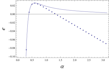
Figure 2: The energy of a finite annular sector, with ratio of inner and outer annular radii $a/b=0.5$, as a function of the wedge angle $\alpha$. The solid curve shows the explicit angular dependence resulting from the subtractions, $w(\alpha)$, while the data points are the total energy obtained by adding $w$ to the numerical integration of the remainder $e_{R}(\alpha)$. It will be noted that below the maximum, the total energy is indistinguishable from that obtained from $w$, while above the maximum, the total energy is asymptotically linear, and deviates significantly from $w$.

The qualitative features hold in every case. The energy is accurately given by $w$ below the point at which the energy reaches a maximum, and above that point, the total energy, which now deviates signficantly from $w$, is very accurately linear. Therefore, to obtain the finite, renormalized energy, we subtract from the energy a fit to this dependence, in accordance with the remarks following Eq. (96). In this way we obtain the results shown in Fig. 3.

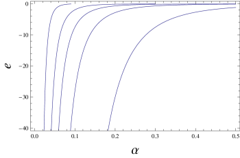
Figure 3: The renormalized energy for the annular sector, obtained by taking the energy $\mathscr{E}^{f}$ and subtracting the linear dependence occuring for sufficiently large angles. Shown, from left to right, are energies for ratios of inner and outer radii, $a/b$, equal to 0.9, 0.7, 0.5, 0.3, and 0.1, respectively.

The energy, the negative gradient of which now unambiguously is the torque on one of the radial planes, is large and negative for small wedge angle $\alpha$ and then rapidly tends to zero. As the ratio $a/b$ gets smaller the region where the attractive torque is significant gets larger. These curves are very similar to those found for an annular piston in Ref. Milton:2009bz , the difference there being that both sides of the radial walls are considered, so $\mathscr{E}(\alpha)\to\mathscr{E}(\alpha)+\mathscr{E}(2\pi-\alpha)$, so a similar attraction appears near $\alpha=2\pi$. Indeed, when a smaller plot range is specified the results agree rather closely with those found in Ref. Milton:2009bz . There, only three-body (wedge-inner cylinder-outer cylinder) effects were considered from the outset. By our process of renormalization we have removed two-body and one-body terms, such as the energy due to the wedge by itself.

VII Discussion

The divergent terms, the pressure anomaly related to the direction of point-splitting, and the ambiguity associated with logarithmic divergences, are present in the energy as linear terms in the wedge angle $\alpha$. Constant terms in $\alpha$, of course, do not contribute to the torque, and linear terms yield a constant torque, that is, one independent of the wedge angle. Any such constant torque has no physical significance and should be subtracted. Indeed, because of the logarithmic divergence associated with curvature, any linear dependence in the wedge angle is ambiguous, and that dependence must be determined by a physical requirement. Here that requirement is supplied by the condition that the energy must vanish for sufficiently large wedge angles. Furthermore, any linear dependence in $\alpha$ would be cancelled if the exterior region of the annular piston were included, for which $\alpha\to 2\pi-\alpha$. For this reason, only the finite, unambiguous, nonlinear dependence in the energy has physical significance. The torque anomaly that appeared for $t$-splitting occurs only in the divergent terms and therefore is removed by the process of renormalization.

Finally, let us make a remark about the situation when there is no inner boundary, so the sector consists of the region $0\leq\rho<b$, $0<\theta<\alpha$. Why could one not proceed as here for the inner radius $a>0$? Then in the divergent terms we would have for the corner divergence

$$\mathscr{E}_{\rm corner\,div}=\mp\frac{C}{48\pi\delta^{2}},$$ (105)

for $z$- and $t$-splitting respectively. Now the corner coefficient contains the apex:

$$C_{\rm apex}=\frac{\pi}{\alpha}-\frac{\alpha}{\pi}.$$ (106)

Now, the divergent terms have a nonlinear dependence on $\alpha$, rendering it impossible to extract a finite energy through “renormalization.” This irreducible singularity presumably is the mirror of the torque anomaly of Ref. fulling12 .

In subsequent papers we will explore the electromagnetic situation, with perfectly conducting boundary conditions, and how these results can be understood from a local analysis of the stress tensor.

References

• (1) S. A. Fulling, F. D. Mera, and C. S. Trendafilova, Phys. Rev. D 87, 047702 (2013) [arXiv:1212.6249].
• (2) J. S. Dowker, “A note on the torque anomaly,” arXiv:1302.1445.
• (3) J. S. Dowker and G. Kennedy, J. Phys. A 11, 895 (1978).
• (4) D. Deutsch and P. Candelas, Phys. Rev. D 20, 3063 (1979).
• (5) I. Brevik and M. Lygren, Ann. Phys. 251, 157 (1996).
• (6) A. A. Saharian and A. S. Tarloyan, Ann. Phys. 323, 1588 (2008).
• (7) R. Estrada, S. A. Fulling, and F. D. Mera, J. Phys. A 45, 455402 (2012) [arXiv:1207.7013 [gr-qc]].
• (8) K. A. Milton, J. Wagner, and K. Kirsten, Phys. Rev. D 80, 125028 (2009) [arXiv:0911.1123 [hep-th]].
• (9) A. P. Prodnikov, Yu. A. Brychkov, and O. I. Marichev, Integrals and Series, vol. 2 (Gordon and Breach, Amsterdam, 1990).
• (10) K. A. Milton, The Casimir Effect (World Singapore, Singapore, 2001).
• (11) C. G. Callan, Jr., S. R. Coleman, and R. Jackiw, Ann. Phys. (N.Y.) 59, 42 (1970).
• (12) K. A. Milton, Phys. Rev. D 4, 3579 (1971).
• (13) K. A. Milton, Lect. Notes Phys.  834, 39 (2011) [arXiv:1005.0031 [hep-th]].
• (14) NIST Digital Library of Mathematical Functions, http://dlmf.nist.gov/, Release 1.0.5 of 2012-10-01.
• (15) S. A. Fulling, J. Phys. A 36, 6857 (2003) [quant-ph/0302117].
• (16) E. K. Abalo, K. A. Milton, and L. Kaplan, Phys. Rev. D 82, 125007 (2010) [arXiv:1008.4778 [hep-th]].
• (17) E. K. Abalo, K. A. Milton, and L. Kaplan, J. Phys. A 45, 425401 (2012) [arXiv:1202.0908 [hep-th]].
• (18) I. S. Gradshteyn and I. M. Ryzhik, Tables of Integrals, Series, and Products, 4th edition (Academic, New York, 1965), 8.526.
• (19) K. Kirsten, J. Phys. A 25, 6297 (1992).
• (20) J. S. Dowker and J. S. Apps, Class. Quant. Grav.  12, 1363 (1995) [hep-th/9502015].
• (21) J. S. Apps and J. S. Dowker, Class. Quant. Grav. 15, 1121 (1998).
• (22) V. V. Nesterenko, I. G. Pirozhenko, and J. Dittrich, Class. Quant. Grav.  20, 431 (2003) [hep-th/0207038].
• (23) K. Kirsten, Spectral Functions in Mathematics and Physics (Chapman and Hall, Boca Raton, 2002).
• (24) P. B. Gilkey, K. Kirsten, and D. V. Vassilevich, Nucl. Phys. B 601, 125 (2001).
• (25) W. Lukosz, Z. Phys. 258, 99 (1973).
• (26) C. M. Bender and P. Hays, Phys. Rev. D 14, 2622 (1976).