Bayesian nonparametric analysis of reversible Markov chains

Abstract

We introduce a three-parameter random walk with reinforcement, called the $(\theta,\alpha,\beta)$ scheme, which generalizes the linearly edge reinforced random walk to uncountable spaces. The parameter $\beta$ smoothly tunes the $(\theta,\alpha,\beta)$ scheme between this edge reinforced random walk and the classical exchangeable two-parameter Hoppe urn scheme, while the parameters $\alpha$ and $\theta$ modulate how many states are typically visited. Resorting to de Finetti’s theorem for Markov chains, we use the $(\theta,\alpha,\beta)$ scheme to define a nonparametric prior for Bayesian analysis of reversible Markov chains. The prior is applied in Bayesian nonparametric inference for species sampling problems with data generated from a reversible Markov chain with an unknown transition kernel. As a real example, we analyze data from molecular dynamics simulations of protein folding.

, and

t1Supported by Grant NIH-R01-GM062868 and NSF Grant DMS-09-00700.

t22Supported by the European Research Council (ERC) through StG “N-BNP” 306406.

1 Introduction

The problem that motivated our study is the analysis of benchtop and computer experiments that produce dynamical data associated with the structural fluctuations of a protein in water. Frequently, the physical laws that govern these dynamics are time-reversible. Therefore, a stochastic model for the experiment should also be reversible. Reversible Markov models in particular have become widespread in the field of molecular dynamics Pande2010 . Modeling with reversible Markov chains is also natural in a number of other disciplines.

We consider the setting in which a scientist has a sequence of states $X_{1},\ldots,X_{n}$ sampled from a reversible Markov chain. We propose a Bayesian model for a reversible Markov chain driven by an unknown transition kernel. Problems one can deal with using our model include (i) predicting how soon the process will return to a specific state of interest and (ii) predicting the number of states not yet explored by $X_{1},\ldots,X_{n}$ that appear in the next $m$ transitions $X_{n+1},\ldots,X_{n+m}$. More generally, the model can be used to predict any characteristic of the future trajectory of the process. Problems (i) and (ii) are of great interest in the analysis of computer experiments on protein dynamics.

Diaconis and Rolles Diaconis2006gd introduced a conjugate prior for Bayesian analysis of reversible Markov chains. This prior is defined via de Finetti’s theorem for Markov chains Diaconis1980hb . The predictive distribution is that of a linearly edge-reinforced random walk (ERRW) on an undirected graph Diaconis1988 . Much is known about the asymptotic properties of this process Keane2000df , its uniqueness Rolles2003xd and its recurrence on infinite graphs (Merkl2009 , and references therein). Fortini, Petrone and Bacallado recently discussed other examples of Markov chain priors constructed through representation theorems fortini2012hierarchical , Bacallado2011 .

Our construction can be viewed as an extension of the ERRW defined on an infinite space. The prediction for the next state visited by the process is not solely a function of the number of transitions observed in and out of the last state. In effect, transition probabilities out of different states share statistical strength. This will become relevant in applications where many states are observed, especially for those states that occur rarely.

A major goal in our application is the prediction of the number of states that the Markov chain has not yet visited that will appear in the next $m$ transitions. More generally, scientists are interested in predicting aspects of the protein dynamics that may be strongly correlated with the rate of discovery of unobserved states, for instance, the variability of the time needed to reach a conformation of interest $y$, starting from a specific state $x$. Predictive distributions for such attributes are useful in deciding whether one should continue a costly experiment to obtain substantial additional information on a kinetic property of interest.

Estimating the probability of discovering new species is a long-standing problem in statistics Bunge1993 . Most contributions in the literature assume that observations, for example, species of fish captured in a lake, can be modeled as independent and identically distributed random variables with an unknown discrete distribution. In this setting, several Bayesian nonparametric models have been studied Lijoi2007a , Lijoi2007b , Favaro2009 . Here we assume that species, in our case protein conformational states, are sampled from a reversible Markov chain. To the best of our knowledge, this is the first Bayesian analysis of species sampling in this setting.

Figure 1: Diagram of the $(\theta,\alpha,\beta)$ scheme and special cases.

We can now outline the article. Section 2 introduces the species sampling model, which we call the $(\theta,\alpha,\beta)$ scheme. The process specializes to the ERRW, a Markov exchangeable scheme, and to the two-parameter Hoppe urn, a classical exchangeable scheme which gives rise to the Pitman–Yor process and the two-parameter Poisson–Dirichlet distribution Pitman1996 , Pitman1997 . As illustrated in Figure 1, the parameter $\beta$ smoothly tunes the model between these two special cases. Section 3 shows that the $(\theta,\alpha,\beta)$ scheme can be represented as a mixture of reversible Markov chains. This allows us to use its de Finetti measure as a prior for Bayesian analysis. Section 4 shows that our scheme is a projection of a conjugate prior for a random walk on a multigraph. This representation is then used to prove that our model has full weak support. Section 5 provides a sufficientness characterization of the proposed scheme. This result is strictly related to the characterizations of the ERRW and the two-parameter Hoppe urn discussed in Rolles2003xd and zabell2005symmetry , respectively. In Section 6, an expression for the law of the $(\theta,\alpha,\beta)$ scheme is derived, and this result is used in Section 7 to define algorithms for posterior simulation. Section 8 applies our model to the analysis of two molecular dynamics datasets. We evaluate the predictive performance of the model by splitting the data into training and validating datasets. Section 9 concludes with a discussion of remaining challenges.

2 The $(\theta,\alpha,\beta)$ scheme

The $(\theta,\alpha,\beta)$ scheme is a stochastic process $(X_{i})_{i\in\mathbb{N}}$ on a Polish measurable space $(\mathcal{X},\mathcal{F})$ equipped with a diffuse (i.e., without point masses) probability measure $\mu$. We construct the law of the process using an auxiliary random walk with reinforcement on the extended space $\mathcal{X}_{+}:=\mathcal{X}\cup\{\zeta\}$. The auxiliary process classifies each transition $X_{i}\to X_{i+1}$ into three categories listed in Figure 2 and defines latent variables $(U_{i})_{i\in\mathbb{N}}$, taking values in $\{a,b,c\}$, that capture each transitions’ category. In this section we first provide a formal definition of the $(\theta,\alpha,\beta)$ scheme and then briefly describe the latent process.

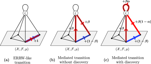
Figure 2: Three kinds of transition in the $(\theta,\alpha,\beta)$ scheme. The blue arrow represents the transition between two states in $\mathcal{X}$, while the red arrows represent the path of an auxiliary random walk with reinforcement. The edges that have positive weight $g$ before the transition are drawn in black, and in each case, we mark the reinforcements of $g$ produced by the transition. Self-transitions follow a slightly different reinforcement scheme formalized in Definition 2.1.

The law of the $(\theta,\alpha,\beta)$ scheme is specified by a weighted undirected graph $g$ with vertices in $\mathcal{X}_{+}$. This graph can be formalized as a symmetric function $g\dvtx\mathcal{X}_{+}\times\mathcal{X}_{+}\to[0,\infty)$, where $g(x,y)$ is the weight of an undirected edge with vertices $x$ and $y$. We require that the set $\mathcal{S}:=\{x\in\mathcal{X};g(\zeta,x)>0\}$ is countable, $\sum_{x\in\mathcal{S}}g(\zeta,x)<\infty$ and that the set of edges $\{(x,y)\in\mathcal{X}^{2};g(x,y)>0\}$ is a finite subset of $\mathcal{S}^{2}$. The graph will be sequentially reinforced after each transition of the $(\theta,\alpha,\beta)$ scheme. In the following definition, we assume the initial state $X_{1}$ is deterministic and contained in $\mathcal{S}$.

Definition 2.1.

The $(\theta,\alpha,\beta)$ scheme, $(X_{i})_{i\in\mathbb{N}}$, has parameters $\theta\geq 0$, $\alpha\in[0,1)$ and $\beta\in[0,1]$. The parameter $\theta$ is equal to the initial weight $g(\zeta,\zeta)$. Suppose we have sampled $X_{1},\ldots,X_{i}$, where $i\geq 1$. Then, given $X_{i}$ and the reinforced graph $g$, we sample the following: [(c)]

an ERRW-like transition to $X_{i+1}$ with probability

$$\frac{g(X_{i},X_{i+1})}{\sum_{x\in\mathcal{X}_{+}}g(X_{i},x)}$$

and make the following reinforcement:

$$g(X_{i},X_{i+1})\to g(X_{i},X_{i+1})+1+\mathbf{1}_{X_{i}=X_{i+1}};$$

a mediated transition without discovery to $X_{i+1}$ with probability

$$\frac{g(X_{i},\zeta)}{\sum_{x\in\mathcal{X}_{+}}g(X_{i},x)}\times\frac{g(\zeta,X_{i+1})+\beta\times\mathbf{1}_{X_{i}=X_{i+1}}}{\beta+\sum_{x\in\mathcal{X}_{+}}g(\zeta,x)}$$

and make the following reinforcements:

$$g(X_{i},X_{i+1}) \to g(X_{i},X_{i+1})+(1-\beta)\times(1+\mathbf{1}_{X_{i}=X_{i+1}}),$$

$$g(X_{i},\zeta) \to g(X_{i},\zeta)+\beta,$$

$$g(X_{i+1},\zeta) \to g(X_{i+1},\zeta)+\beta;$$

a mediated transition with discovery to a new state $X_{i+1}\sim\mu$ with probability

$$\frac{g(X_{i},\zeta)}{\sum_{x\in\mathcal{X}_{+}}g(X_{i},x)}\times\frac{g(\zeta,\zeta)}{\beta+\sum_{x\in\mathcal{X}_{+}}g(\zeta,x)}$$

and make the following reinforcements:

$$g(X_{i},X_{i+1}) \to g(X_{i},X_{i+1})+(1-\beta),$$

$$g(X_{i},\zeta) \to g(X_{i},\zeta)+\beta,$$

$$g(X_{i+1},\zeta) \to g(X_{i+1},\zeta)+(1-\alpha)\beta,$$

$$g(\zeta,\zeta) \to g(\zeta,\zeta)+\alpha\beta.$$

In several applications one may prefer to set the initial $g$ to zero everywhere except for $g(\zeta,\zeta)=\theta$ and $g(X_{1},\zeta)$, which can be made infinitesimally small. This reduces difficulties associated with the model specification and does not affect the main properties of the model discussed in this article. In some cases, we will relax the assumption that $X_{1}$ is deterministic, by specifying a distribution, say $\mu$, for $X_{1}$ and choosing a positive value for $g(X_{1},\zeta)$. In any case, the conditional distributions $p(X_{n}|X_{1},\ldots,X_{n-1})$ are dictated by the reinforced scheme in Definition 2.1.

We can now describe the latent reinforced process in order to simplify the interpretation of the $(\theta,\alpha,\beta)$ scheme. To sample a transition $X_{i}\to X_{i+1}$, we first take one step in the auxiliary random walk from $X_{i}$. If we land on a state $x\in\mathcal{X}$ [panel (a) in Figure 2], we set $X_{i+1}=x$ and $U_{i}=a$. If we land on $\zeta$, we sample another step of the random walk from $\zeta$. Once more, if we land on some $x^{\prime}\in\mathcal{X}$ [panel (b) in Figure 2], we set $X_{i+1}=x^{\prime}$ and $U_{i}=b$. Otherwise [panel (c) in Figure 2], we sample a new state $X_{i+1}$ from $\mu$ and set $U_{i}=c$.

Remark 2.1.

Assume the initial graph $g$ is null everywhere except for $g(\zeta,\zeta)=\theta$ and $g(\zeta,X_{1})=1$. If $\beta=1$, $\alpha=0$ and $X_{1}\sim\mu$, then the process $(X_{i})_{i\in\mathbb{N}}$ is a Blackwell–MacQueen urn Blackwell1973 with base distribution $\mu$ and concentration parameter $\theta/2$. In different words, the process is exchangeable and its directing random measure is the Dirichlet process Ferguson1973 .

Remark 2.2.

Under the assumptions in Remark 2.1, by setting $\alpha>0$ and $g(\zeta,X_{1})=1-\alpha$, the process $(X_{i})_{i\in\mathbb{N}}$ is equal to an urn scheme introduced by Engen Engen1978 , known in the species sampling context as the two-parameter Hoppe urn; see Appendix B supplement . This exchangeable process has been studied extensively by Pitman and Yor Pitman1996 , Pitman1997 . Its directing random measure is the Pitman–Yor process Ishwaran2001 with base distribution $\mu$, concentration parameter $(\theta-\alpha)/2$, and discount parameter $\alpha/2$; the sorted masses of this random measure have the two-parameter Poisson–Dirichlet distribution. Note that the discount parameter of the Pitman–Yor process can be chosen from the unit interval $[0,1)$, while in our construction $\alpha/2<0.5$.

Remark 2.3.

When $\beta=\theta=0$, edges connected to $\zeta$ cannot be reinforced, and the $(\theta,\alpha,\beta)$ scheme specializes to the ERRW on $\mathcal{S}$; see Diaconis1988 .

Remark 2.4.

Definition 2.1 brings to mind the two-parameter hierarchical Dirichlet Process hidden Markov model (HDP-HMM) teh2010hierarchical and its associated species sampling scheme, the two-parameter Chinese restaurant franchise. This process has been used for Bayesian modeling of Markov chains on infinite spaces. The predictive distribution can be viewed as a $(\theta,\alpha,\beta)$ scheme in which the underlying infinite graph has directed edges. However, the $(\theta,\alpha,\beta)$ scheme is not a special case of this model and has no equivalent hierarchical construction. This connection is explained in more detail in Appendix B supplement .

The influence of each parameter in the $(\theta,\alpha,\beta)$ scheme can be described as follows. The parameter $\beta$ determines the Markov character of the model; as it approaches 1, the process becomes exchangeable. The parameter $\theta$ is related to the concentration parameter of the two-parameter Hoppe urn, which controls the mode of the number of states visited in a given number of steps. The parameter $\alpha$ is related to the discount factor in the two-parameter Hoppe urn, which controls the distribution of frequencies of different states. It is worth noting that $\beta$ also controls the number of states visited, which increases markedly as $\beta$ is made larger.

The recurrence of the ERRW on infinite graphs is far from trivial, especially for locally connected graphs (Merkl2009 , and references therein). However, it is not difficult to prove that the $(\theta,\alpha,\beta)$ scheme a.s. returns infinitely often to all visited states, the state $\zeta$ is visited infinitely often a.s. and, if $\theta>0$, the edge $g(\zeta,\zeta)$ is crossed infinitely often. This notion of recurrence is stated in the next proposition.

Proposition 2.1

The $(\theta,\alpha,\beta)$ scheme is recurrent, that is, the event $\{\sum_{j>i}\mathbf{1}_{X_{i}=X_{j}}>0\}$ has probability 1 for every integer $i$. When $\theta>0$ or when the set $\mathcal{S}$ is infinite, the number of states visited is infinite almost surely.

3 de Finetti representation of the $(\theta,\alpha,\beta)$ scheme

Diaconis and Freedman defined a special notion of partial exchangeability to prove a version of de Finetti’s theorem for Markov chains Diaconis1980hb .

Definition 3.1.

A stochastic process on a countable space $\mathcal{X}$ is Markov exchangeable if the probability of observing a path $x_{1},\ldots,x_{n}$ is only a function of $x_{1}$ and the transition counts $C(x,y):=|\{x_{i}=x,x_{i+1}=y;1\leq i<n\}|$ for all $x,y\in\mathcal{X}$.

Theorem 3.1 ((Diaconis and Freedman))

A process is Markov exchangeable and returns to every state visited infinitely often, if and only if it is a mixture of recurrent Markov chains.

The $(\theta,\alpha,\beta)$ scheme takes values in an uncountable space $\mathcal{X}$, which precludes a direct application of Theorem 3.1. We will state a more general notion of Markov exchangeability and use it to prove a de Finetti style representation for $(X_{i})_{i\in\mathbb{N}}$. We use the notion of $x$-block defined in Diaconis and Freedman Diaconis1980hb ; given a recurrent trajectory $x_{1},x_{2},\ldots\,$, the $i$th $x$-block, for any state $x$ appearing in $x_{1},x_{2},\ldots\,$, is the finite subsequence that starts with the $i$th occurrence of $x$ and ends before the $(i+1)$th occurrence.

The process $(X_{i})_{i\in\mathbb{N}}$ visits every state in $\mathcal{S}$ infinitely often; in addition, it will discover new species in $\mathcal{X}$ in steps of the third kind in Figure 2. But the new species are sampled independently from $\mu$, which motivates expressing $(X_{i})_{i\in\mathbb{N}}$ as a function of two independent processes on the same probability space: $(Z_{i})_{i\in\mathbb{N}}$ which represents the sequence where new species are labeled in order of appearance, and $(T_{i})_{i\in\mathbb{N}}$ which represents the $\mathcal{X}$-valued locations of each species. These are formally defined in the sequel.

Let $\mathcal{Z}=\mathcal{X}\sqcup\mathbb{N}$, and let $d$ be a function that maps a sequence in $\mathcal{Z}\supset\mathcal{S}$ to a sequence in the disjoint union $\mathcal{S}\sqcup\mathbb{N}$. Each element of the sequence in $\mathcal{S}$ is mapped to itself, and those not in $\mathcal{S}$ are mapped to the order in which they appear in the sequence. Hence, the range of $d$ consists of sequences where every state $j\in\mathbb{N}$ may only appear after all states $1,2,\ldots,j-1$ have appeared at least once. For example, if $\mathcal{X}$ is the unit interval and $\mathcal{S}=\{0.1,0.2,0.3\}$, then

$$d\dvtx(0.1,7,4,0.3,7,6,4,4)\mapsto(0.1,1,2,0.3,1,3,2,2).$$

Define $(Z_{i})_{i\in\mathbb{N}}:=d((X_{i})_{i\in\mathbb{N}})$, and let $(T_{i})_{i\in\mathbb{N}}$ be a sequence of independent random variables from $\mu$, with $(T_{i})_{i\in\mathbb{N}}$ independent from $(Z_{i})_{i\in\mathbb{N}}$. Then,

$$(X_{i})_{i\in\mathbb{N}}\stackrel{{\scriptstyle\mathrm{d}}}{{=}}(\bar{X}_{i})_{i\in\mathbb{N}}\qquad\mbox{where we define }\bar{X}_{i}:=\cases{Z_{i},&\quad if $Z_{i}\in\mathcal{S}$,\cr T_{Z_{i}},&\quad otherwise.}$$

Proposition 3.1

Take two sequences $x_{1},\ldots,x_{n}$ and $x^{\prime}_{1},\ldots,x^{\prime}_{n}$ in $\mathcal{S}\sqcup\mathbb{N}$ that are fixed points of $d$. Suppose one can map $x_{1},\ldots,x_{n}$ to $x^{\prime}_{1},\ldots,x^{\prime}_{n}$ by a transposition of two blocks in $x_{1},\ldots,x_{n}$ which both begin in $x\in\mathcal{S}\sqcup\mathbb{N}$ and end in $y\in\mathcal{S}\sqcup\mathbb{N}$, followed by an application of the mapping $d$. Then,

$$p(Z_{1}=x_{1},\ldots,Z_{n}=x_{n})=p\bigl{(}Z_{1}=x^{\prime}_{1},\ldots,Z_{n}=x^{\prime}_{n}\bigr{)}.$$

Example 3.1.

Assume again $\mathcal{S}=\{0.1,0.2,0.3\}$. If we set

$$(x_{1},\ldots,x_{n})=(0.1,1,2,0.3,3,2,4,0.3)$$

and

$$\bigl{(}x^{\prime}_{1},\ldots,x^{\prime}_{n}\bigr{)}=(0.1,1,2,3,0.3,4,2,0.3),$$

then, by transposing two blocks in $(x_{1},\ldots,x_{n})$ that start from $2$ and finish in $0.3$, we obtain the vector $(0.1,1,2,4,0.3,3,2,0.3)$. Moreover,

$$d(0.1,1,2,4,0.3,3,2,0.3)=(0.1,1,2,3,0.3,4,2,0.3)=\bigl{(}x^{\prime}_{1},\ldots,x^{\prime}_{n}\bigr{)}.$$

Proposition 3.1 then implies that the two probabilities, $p(Z_{1}=x_{1},\ldots,Z_{n}=x_{n})$ and $p(Z_{1}=x^{\prime}_{1},\ldots,Z_{n}=x^{\prime}_{n})$, are identical.

Remark 3.1.

Note that if the process only visits states in $\mathcal{S}$, as is the case when $\theta=0$, the statement of Proposition 3.1 is equivalent to Markov exchangeability; cf. Proposition 27 in Diaconis1980hb . This fact, together with Proposition 2.1 is enough to show by a straightforward application of Theorem 3.1 that the $(\theta,\alpha,\beta)$ scheme with $\theta=0$ is a mixture of recurrent Markov chains on $\mathcal{S}$.

Equipped with this notion of Markov exchangeability for the species sampling sequence $(Z_{i})_{i\in\mathbb{N}}$, we show that $(X_{i})_{i\in\mathbb{N}}$ can be represented as a mixture of Markov chains.

Proposition 3.2

There exists a mixture of Markov chains $(W_{i})_{i\in\mathbb{N}}$, taking values in $\mathcal{S}\sqcup\mathbb{N}$, such that, if we define

$$\tilde{X}_{i}:=\cases{W_{i},&\quad if $W_{i}\in\mathcal{S}$,\cr T_{W_{i}},&\quad otherwise,}$$

where $(W_{i})_{i\in\mathbb{N}}$ and $(T_{i})_{i\in\mathbb{N}}\sim\mu^{\mathbb{N}}$ are independent, then $(\tilde{X}_{i})_{i\in\mathbb{N}}\stackrel{{\scriptstyle\mathrm{d}}}{{=}}(X_{i})_{i\in\mathbb{N}}$. That is, for some measure $\phi$ on $(\mathcal{S}\sqcup\mathbb{N})\times\mathcal{P}$, where $\mathcal{P}$ is the space of stochastic matrices on $\mathcal{S}\sqcup\mathbb{N}$, the distribution of $(W_{i})_{i\in\mathbb{N}}$, can be represented as

$$p(W_{1}=w_{1},\ldots,W_{n}=w_{n})=\int_{\mathcal{P}}\prod_{i=1}^{n-1}P(w_{i},w_{i+1})\phi(w_{1},dP).$$

Let $\mathcal{P}_{r}\subset\mathcal{P}$ be the set of transition probability matrices for recurrent reversible Markov chains. We can show that this set has probability 1 under the de Finetti measure.

Proposition 3.3

$\phi((\mathcal{S}\sqcup\mathbb{N})\times\mathcal{P}_{r})=1$.

4 The $(\theta,\alpha,\beta)$ scheme with colors

This section shows that the $(\theta,\alpha,\beta)$ scheme can be interpreted as a Bayesian conjugate model for a random walk on a multigraph. This representation is used for showing that the $(\theta,\alpha,\beta)$ scheme has large support in a sense that will be made precise in the sequel. We also make a connection between the de Finetti measure of the ERRW on a finite graph and our model.

We start by defining a colored random walk on a weighted multigraph $\tilde{g}$. The vertices of the graph take values in $\mathcal{X}$, and we now allow there to be more than one edge between every pair of vertices. Every edge is associated to a distinct color in a set $\mathcal{C}$. We assign a weight $\tilde{g}(\{x,y\},c)$ to the edge connecting $x$ and $y$ with color $c$, requiring that $\tilde{g}(x):=\sum_{y,c}g(\{x,y\},c)<\infty$ for all $x\in\mathcal{X}$. A random walk on this graph is a process that starts from $x_{1}\in\mathcal{X}$, and after arriving at some state $x$, traverses the edge $(\{x,z\},c)$ with probability $\tilde{g}(\{x,z\},c)/\tilde{g}(x)$. Let $p_{\tilde{g}}$ be the law of this process.

A Bayesian statistician observes a finite sequence of traversed colored edges and wants to predict the future trajectory of the colored random walk. We suggest how to use the $(\theta,\alpha,\beta)$ scheme in this context. Informally, in a ERRW-like transition, we reinforce a single edge of a specific color, while in a mediated transition, we draw a new edge with a novel color.

The Bayesian model is a random sequence of colored edges $(E_{i})_{i\in\mathbb{N}}$. We use $C_{i}$ and $\{X_{i},X_{i+1}\}$ to denote the color and vertices of $E_{i}$. Let $\mu$ and $\gamma$ be nonatomic distributions over $\mathcal{X}$ and $\mathcal{C}$, respectively, and specify $\theta$, $\alpha$ and $\beta$ as in the previous sections. Let $X_{1}=x_{1}$, $C_{1}\sim\gamma$ and

$$X_{2}|X_{1},C_{1}\sim\frac{\beta(1-\alpha)}{\beta+\theta}\bolds{\delta}_{X_{1}}+\frac{\theta+\alpha\beta}{\beta+\theta}\mu.$$

The distribution of $(X_{1},X_{2})$ corresponds to an initial graph with only 2 edges, with endpoints $\{x_{1},\zeta\}$ and $\{\zeta,\zeta\}$, weighted by $-\alpha\beta$ and $\theta+\alpha\beta$, respectively. If the initial weighted graph $g$ in a $(\theta,\alpha,\beta)$ scheme is chosen as above, the reinforcement rules in Definition 2.1 produce a well-defined process even if the initial value of $g(x_{1},\zeta)$ is negative. After the first transition all edges will have nonnegative weights. This choice for the initial weighted graph will be used in the present section and Section 5.

After a path $(E_{1},\ldots,E_{n})$, the probability of recrossing an edge $E_{j}$, with $j\leq n$ and $X_{n+1}\in\{X_{j},X_{j+1}\}$, is

$$p(E_{n+1}=E_{j}|E_{1},\ldots,E_{n})=\frac{G_{n}(\{X_{j},X_{j+1}\},C_{j})}{W_{X_{n+1},n}},$$

where

$$G_{n}\bigl{(}\{x,y\},c\bigr{)} = \max\biggl{(}0,-\beta+\sum_{i\leq n}\mathbf{1}_{E_{i}=(\{x,y\},c)}\biggr{)}2^{\mathbf{1}_{x=y}},$$

$$W_{x,n} = -\alpha\beta+\sum_{i\leq n}(\mathbf{1}_{x\in\{X_{i},X_{i+1}\}})2^{\mathbf{1}_{X_{i}=X_{i+1}}}.$$

In words, the probability of recrossing an edge is linear in the number of crossings. Let $\mathcal{C}_{n}$ be the set of distinct colors in $(C_{1},\ldots,C_{n})$. The conditional probability that $C_{n+1}\notin\mathcal{C}_{n}$,

$$p(C_{n+1}\notin\mathcal{C}_{n}|E_{1},\ldots,E_{n})=\frac{B_{X_{n+1},n}}{W_{X_{n+1},n}},$$

where

$$B_{x,n}=-\alpha\beta+\beta\sum_{i\leq n}(\mathbf{1}_{x\in\{X_{i},X_{i+1}\}})(\mathbf{1}_{C_{i}\notin\mathcal{C}_{i-1}})2^{\mathbf{1}_{X_{i}=X_{i+1}}}$$

is linear in the number of distinct colored edges adjacent to $X_{n+1}$. The probability that $X_{n+2}=y$, for any vertex $y\in\{X_{1},\ldots,X_{n}\}$, conditional on $C_{n+1}\notin\mathcal{C}_{n}$, is

$$p(X_{n+2}=y|E_{1},\ldots,E_{n},C_{n+1}\notin\mathcal{C}_{n})=\frac{\beta\mathbf{1}_{X_{n+1}=y}+B_{y,n}}{2\beta\times|\mathcal{C}_{n}|+\theta+\beta},$$ (1)

which depends linearly on the number of distinct colored edges adjacent to $y$. Finally,

$$X_{n+2}|C_{n+1}\notin\mathcal{C}_{n},\qquad X_{n+2}\notin\{X_{1},\ldots,X_{n+1}\},\qquad E_{1},\ldots,E_{n}\sim\mu$$

and

$$C_{n+1}|X_{n+2},\qquad E_{1},\ldots,E_{n},\qquad C_{n+1}\notin\mathcal{C}_{n}\sim\gamma.$$

The following property is a direct consequence of this definition.

Proposition 4.1

The sequence $(X_{i})_{i\in\mathbb{N}}$ of $\mathcal{X}$-valued states visited by $(E_{i})_{i\in\mathbb{N}}$ is identical in distribution to a $(\theta,\alpha,\beta)$ scheme initiated at $x_{1}$, with $g$ everywhere null except at $g(x_{1},\zeta)=-\beta\alpha$ and $g(\zeta,\zeta)=\theta+\alpha\beta$.

Furthermore, given a $(\theta,\alpha,\beta)$ scheme with an arbitrary initial graph $g$, it is possible to construct a colored $(\theta,\alpha,\beta)$ scheme with a closed-form predictive distribution such that the equality stated in Proposition 4.1 holds. This would require changing the definition of $(E_{i})_{i\in\mathbb{N}}$ in a way that preserves the reinforcement scheme.

Proposition 4.2

Let $e_{1},\ldots,e_{n}$ be a colored path, with $e_{i}=(\{x_{i},x_{i+1}\},\allowbreak c_{i})$, and let $\Lambda(e_{1},\ldots,e_{n})$ be the probability of the event

$$\bigcap_{e_{i}=e_{j}}\{E_{i}=E_{j}\}\bigcap_{e_{i}\neq e_{j}}\{E_{i}\neq E_{j}\}\bigcap_{x_{i}=x_{j}}\{X_{i}=X_{j}\}\bigcap_{x_{i}\neq x_{j}}\{X_{i}\neq X_{j}\}.$$

Suppose $e_{\sigma(1)},\ldots,e_{\sigma(n)}$, for some permutation $\sigma$, is also a colored path starting at $x_{1}$. Then,

$$\Lambda(e_{1},\ldots,e_{n})=\Lambda(e_{\sigma_{1}},\ldots,e_{\sigma_{n}}).$$ (2)

This result, related to Proposition 3.1, establishes a probabilistic symmetry between paths that can be mapped to each other by permuting the order of edges crossed, and applying certain automorphisms to $\mathcal{X}$ and $\mathcal{C}$. Proposition 4.2 gives rise to the following de Finetti representation.

Proposition 4.3

There exists a mixture of colored random walks on weighted multigraphs $(\{W_{i},W_{i+1}\},J_{i})_{i\in\mathbb{N}}$, with $W_{i}\in\mathbb{N}$ and $J_{i}\in\mathbb{N}$, and independent processes $(T_{i})_{i\in\mathbb{N}}\sim\mu^{\mathbb{N}}$ and $(V_{i})_{i\in\mathbb{N}}\sim\gamma^{\mathbb{N}}$, such that the sequence of colored edges $(\{\tilde{X}_{i},\tilde{X}_{i+1}\},\tilde{C}_{i})_{i\in\mathbb{N}}$, defined by

$$(\tilde{X}_{i},\tilde{C}_{i})=\cases{(x_{1},V_{J_{i}}),&\quad if $W_{i}=1$,\cr(T_{W_{i}},V_{J_{i}}),&\quad if $W_{i}>1$,}$$

is identical in distribution to $(E_{i})_{i\in\mathbb{N}}$.

The proof of Proposition 4.3 constructs the discrete process $(W_{i},J_{i})_{i\in\mathbb{N}}$, which will now be used to show that the $(\theta,\alpha,\beta)$ scheme has large support. The law of $(W_{i},J_{i})_{i\in\mathbb{N}}$ can be mapped bijectively to the exchangeable law of the sequence of $x_{1}$-blocks in the process, which in the present section and the next are defined as sequences of labeled edges. Therefore, the de Finetti measure of $(W_{i},J_{i})_{i\in\mathbb{N}}$ uniquely identifies the de Finetti measure of the $x_{1}$-blocks, and vice versa. We denote the random distribution of the $x_{1}$-blocks $\eta$. Note that the space of $x_{1}$-blocks is discrete because $W_{i}$ and $J_{i}$ are integer-valued.

We show that the law of $\eta$ has full weak support. On the basis of Proposition 4.1, we then conclude that the $x_{1}$-block de Finetti measure induced by the $(\theta,\alpha,\beta)$ scheme also has full weak support. The next proposition is proven for $(E_{i})_{i\in\mathbb{N}}$ as defined in this section; the result can be extended to any analogous reinforced process corresponding to a specific $(\theta,\alpha,\beta)$ scheme.

Proposition 4.4

Let $\eta^{o}$ be the $x_{1}$-block distribution induced by a colored random walk on an arbitrary weighted multigraph with vertices and colors in $\mathbb{N}$, in which the sum of weights is finite, $\sum_{x\in\mathbb{N}}\tilde{g}(x)<\infty$. For every $\varepsilon>0$, $m\geq 1$ and any collection of bounded real functions $f_{1},\ldots,f_{m}$ on the space of $x_{1}$-blocks,

$$p\bigl{(}\eta\in U_{\varepsilon,f_{1},\ldots,f_{m}}\bigl{(}\eta^{o}\bigr{)}\bigr{)}>0,$$

where

$$U_{\varepsilon,f_{1},\ldots,f_{m}}\bigl{(}\eta^{o}\bigr{)}=\biggl{\{}\eta^{\prime}\dvtx\biggl{|}\int f_{i}\,d\eta^{o}-\int f_{i}\,d\eta^{\prime}\biggr{|}<\varepsilon,i=1,\ldots,m\biggr{\}}.$$

The process $(E_{i})_{i\in\mathbb{N}}$ also reveals a connection between the $(\theta,\alpha,\beta)$ scheme and the ERRW. Recall that the colored $x_{1}$-blocks $(H_{i})_{i\in\mathbb{N}}$ in the Bayesian model are exchangeable and, by de Finetti’s theorem, conditionally independent. Consider their posterior distribution given the subsequence $(E_{i})_{i\leq n}$, and assume it has $X_{n+1}=X_{1}$ and includes $k$ colored $x_{1}$-blocks. These assumptions are only made to simplify the exposition. The limits

$$T_{(\{x,y\},c)}=\lim_{m\to\infty}\biggl{(}\frac{\sum_{i=n}^{n+m}\mathbf{1}_{(\{X_{i},X_{i+1}\},C_{i})=(\{x,y\},c)}}{\sqrt{\sum_{i=n}^{n+m}\mathbf{1}_{X_{i}=x}}\sqrt{\sum_{i=n}^{n+m}\mathbf{1}_{X_{i}=y}}}\biggr{)}$$ (3)

for every edge $(\{x,y\},c)\in\{E_{1},\ldots,E_{n}\}$ are functions of the directing random measure for the sequence of $x_{1}$-blocks. From these limits, one can obtain the probability in the directing random measure of any $x_{1}$-block formed with edges in $\{E_{1},\ldots,E_{n}\}$. Namely, given $E_{1},\ldots,E_{n}$ and the tail $\sigma$-field of $(E_{i})_{i\in\mathbb{N}}$, the probability of an $x_{1}$-block $e_{1},\ldots,e_{k}$ is the product $\prod_{i=1}^{k}T_{e_{i}}$. We can now state the connection with the ERRW.

Proposition 4.5

There exists an ERRW on a multigraph with a finite number of edges, such that the joint posterior distribution of the random variables in (3), given $E_{1},\ldots,E_{n}$, is identical to the distribution of the same limits in the ERRW.

Appendix C supplement contains a constructive proof of this proposition, in which one such ERRW, whose parameters depend on $E_{1},\ldots,E_{n}$, is defined.

5 Sufficientness characterization

This section provides a characterization of the colored $(\theta,\alpha,\beta)$ scheme in terms of certain predictive sufficiencies or sufficientness conditions. The first characterization of this type, for the Pólya urn, was proven in an influential paper by Johnson Zabell1982ir and has since been extended to other predictive schemes for discrete sequences such as the two-parameter Hoppe urn zabell2005symmetry and the edge-reinforced random walk Rolles2003xd . Our result is closely related to the work of these authors and uses similar proof techniques. In addition to its clear subjective motivation, the characterization elucidates connections between the $(\theta,\alpha,\beta)$ scheme and other popular nonparametric Markov models fortini2012hierarchical .

Consider a random sequence of colored edges $(\tilde{E}_{i})_{i\in\mathbb{N}}$, where $\tilde{E}_{i}=(\{X_{i},\break X_{i-1}\},C_{i})$. Each color in $(\tilde{E}_{i})_{i\in\mathbb{N}}$ identifies an edge. We assume $(\tilde{E}_{i})_{i\in\mathbb{N}}$ is a mixture of random walks on weighted and colored multigraphs, in the sense of Proposition 4.3, which visits more than 2 vertices with probability 1. It will be shown that, if the predictive distribution of $(\tilde{E}_{i})_{i\in\mathbb{N}}$ satisfies certain conditions, then the process is a $(\theta,\alpha,\beta)$ scheme.

Consider a path $Z_{n}=(\tilde{E}_{1},\ldots,\tilde{E}_{n})$ and define:

$$\mbox{(i)}\hskip 10.4pt\quad\kappa(Z_{n}) = \bigl{|}\{0\leq i\leq n;X_{i}=X_{n}\}\bigr{|}+\frac{\mathbf{1}_{X_{n}\neq X_{0}}}{2},$$

$$\mbox{(ii)}\quad\kappa(e,Z_{n}) = \bigl{|}\{1\leq i\leq n;\tilde{E}_{i}=e\}\bigr{|}\quad\mbox{and}$$

$$\mbox{(iii)}\hskip 10.75pt\quad\tau(Z_{n}) = \sum_{v}\eta(v,Z_{n})/2$$

(iv) $$\mbox{where }\eta(v,Z_{n})=\sum_{i\leq n}(\mathbf{1}_{v\in\{X_{i},X_{i+1}\}})(\mathbf{1}_{C_{i}\notin\{C_{1},\ldots,C_{i-1}\}})2^{\mathbf{1}_{X_{i}=X_{i+1}}}.$$

These variables describe: (i) how many times $X_{n}$ has been visited and whether it coincides with $X_{0}$, (ii) how many times an edge $e$ has been traversed, (iii) the number of observed colors and (iv) the degree of $v\in\mathcal{X}$ in the multigraph constructed by all distinct colored edges in $Z_{n}$. In summary, they are easily interpretable. We also use $\rho(Z_{n})$ to denote the number of distinct $\mathcal{X}$-valued states in $Z_{n}$, and the indicator $s(e)$, which is equal to 1 if $e$ is a loop and $0$ otherwise.

We can now define sufficientness conditions for $(\tilde{E}_{i})_{i\in\mathbb{N}}$. The process satisfies Condition 1 if there exist functions $b_{0}$ and $b_{1}$ such that for every $e\in\{\tilde{E}_{1},\ldots,\tilde{E}_{n}\}$ incident on $X_{n}$,

$$p(\tilde{E}_{i+1}=e|Z_{n})=b_{s(e)}\bigl{(}\kappa(Z_{n}),\kappa(e,Z_{n})\bigr{)}\in(0,1).$$ (4)

In words, the probability of making a transition through an edge $e=(\{X_{n},v\},\break c)$ in $Z_{n}$ depends on the number of times the edge has been crossed and the number of visits to $X_{n}$. The process satisfies Condition 2 if there is a function $g$ such that

$$p\bigl{(}\tilde{E}_{n+1}\notin\{\tilde{E}_{1},\ldots,\tilde{E}_{n}\}|Z_{n}\bigr{)}=g\bigl{(}\kappa(Z_{n}),\eta(X_{n},Z_{n})\bigr{)}\in(0,1).$$ (5)

That is, the probability of a transition through a new edge is a function of the number of observed edges $\eta(X_{n},Z_{n})$ incident on $X_{n}$, and the number of visits to $X_{n}$. Condition 3 requires that some function $h$ satisfies, for every $v\in\{X_{0},\ldots,X_{n}\}$,

$$p\bigl{(}X_{i+1}=v|Z_{n},\tilde{E}_{n+1}\notin\{\tilde{E}_{1},\ldots,\tilde{E}_{n}\}\bigr{)}$$

(6)

$$\qquad=h\bigl{(}\tau(Z_{n}),\eta(v,Z_{n})+\mathbf{1}_{X_{n}=v}\bigr{)}\in(0,1).$$

If a new edge will be traversed, then the conditional probability that the path will go to an already seen vertex depends solely on the number of edges out of said vertex and the overall number of observed edges. Finally, the process satisfies Condition 4 if there is a function $q$, such that

$$p\bigl{(}X_{i+1}\notin\{X_{0},\ldots,X_{n}\}|Z_{n},\tilde{E}_{n+1}\notin\{\tilde{E}_{1},\ldots,\tilde{E}_{n}\}\bigr{)}$$

(7)

$$\qquad=q\bigl{(}\tau(Z_{n}),\rho(Z_{n})\bigr{)}\in(0,1);$$

that is, the conditional probability that the path will go to an unseen vertex is a function of the total number of edges and vertices.

The main result of this section can be divided into two lemmas, the first of which depends only on 3 of the conditions above.

Lemma 5.1

If the process $(\tilde{E}_{i})_{i\in\mathbb{N}}$ satisfies Conditions 1, 2 and 3, there exist $\beta\in[0,1)$ and $\lambda\in[-\beta,\infty)$ such that

$$b_{s}(k,j)=\frac{(1+s)(j-\beta)}{\lambda+2k-2}\quad\mbox{and}\quad g(k,t)=\frac{\lambda+\beta t}{\lambda+2k-2}.$$ (8)

Lemma 5.2

If the process $(\tilde{E}_{i})_{i\in\mathbb{N}}$ satisfies Conditions 1, 2, 3 and 4, there exist $\alpha\in[0,1)$ and $\lambda^{\prime}\in[-\alpha,\infty)$ such that

$$h(n,j)=\frac{j-\alpha}{\lambda^{\prime}+2n+1-\alpha}\quad\mbox{and}\quad q(n,t)=\frac{\lambda^{\prime}+\alpha(t-1)}{\lambda^{\prime}+2n+1-\alpha}$$ (9)

for $n=1,2,\ldots\,$, $j=1,\ldots,2n$ and $t=2,\ldots,n+1$.

The characterization of the $(\theta,\alpha,\beta)$ scheme with colors follows from the two previous lemmas.

Theorem 5.1

If the process $(\tilde{E}_{i})_{i\in\mathbb{N}}$ satisfies Conditions 1, 2, 3 and 4, then there exist $\alpha\in[0,1)$, $\beta\in[0,1)$ and $\theta>-2\alpha\beta$, such that the conditional transition probabilities of the process $(\tilde{E}_{i})_{i\in\mathbb{N}}$, given any path that visits more than 2 vertices, are equal to those in the $(\theta,\alpha,\beta)$ scheme with colors $(E_{i})_{i\in\mathbb{N}}$.

6 The law of the $(\theta,\alpha,\beta)$ scheme

We provide an expression for the law of the species sampling sequence $(Z_{i})_{i\in\mathbb{N}}$, defined in Section 3. Recall that the process takes values on $\mathcal{S}\sqcup\mathbb{N}$, and consider a fixed path $\mathbf{z}$.

Let $n_{xy}$ be the number of transitions in $\mathbf{z}$ between $x$ and $y$ in either direction and $n_{x}=\sum_{y\in\mathcal{S}\sqcup\mathbb{N}}n_{xy}$. For each pair $x,y\in\mathcal{S}\sqcup\mathbb{N}$, we introduce $k_{xy}\leq n_{xy}$ for the number of ERRW-like transitions [panel (a), Figure 2] between $x$ and $y$ in either direction. Let $\ell_{x}:=\sum_{y\in\mathcal{S}\sqcup\mathbb{N}}(n_{xy}-k_{xy})2^{\mathbf{1}_{x=y}}$ be the number of times that the latent path traverses the edge $(\zeta,x)$ in either direction, let $\ell:=\sum_{x\in\mathcal{S}\sqcup\mathbb{N}}\ell_{x}/2$ be the number of mediated transitions, and let $\ell^{\prime}$ be the number of times that $(\zeta,\zeta)$ is traversed. Note that $\ell$, $\ell_{x}$ and $\ell^{\prime}$ are functions of $\mathbf{z}$ and $\mathbf{k}=\{k_{xy};x,y\in\mathcal{S}\sqcup\mathbb{N}\}$. We will also need $g(x)=\sum_{y\in\mathcal{S}}g(x,y)$, where $g$ is the initial weighted graph.

Given $\mathbf{k}$ and $\mathbf{z}$, we know the number of transitions out of $\zeta$ and out of $x\in\mathcal{S}\sqcup\mathbb{N}$ in the latent path. Each transition adds a factor to the denominator of the probability of a latent path, which increase by a fixed amount, $2\beta$ or $2$, between occurrences. Similarly, given $\mathbf{k}$, we know the number of times that $(\zeta,x)$ is traversed; each transition adds a factor in the numerator, and these factors are sequentially reinforced by a fixed amount $\beta$. Finally, $(\zeta,\zeta)$ is traversed $\ell^{\prime}$ times, and this contributes a factor $\theta(\theta+\alpha\beta)\cdots(\theta+[\ell^{\prime}-1]\alpha\beta)$ to the numerator of the probability of the latent path.

We can write $p(\mathbf{z})=\sum_{\mathbf{k}}p(\mathbf{z},\mathbf{k})$, where $p(\mathbf{z},\mathbf{k})$ is the total probability of all latent paths consistent with $(\mathbf{z},\mathbf{k})$. Taking into account that the factors listed in the previous paragraph are common to all latent paths with a given $(\mathbf{z},\mathbf{k})$, we obtain

$$p(\mathbf{z},\mathbf{k}) = F(\mathbf{z},\mathbf{k})(\theta)_{\ell^{\prime}\uparrow\alpha\beta}\prod_{x:n_{x}>0}\bigl{(}g(x,\zeta)+\beta(1-\alpha)\mathbf{1}_{x\in\mathbb{N}}\bigr{)}_{\ell_{x}-\mathbf{1}_{x\in\mathbb{N}}\uparrow\beta}$$

$${}\Big{/}\biggl{(}\bigl{(}g(\zeta)+\beta\bigr{)}_{{\ell}\uparrow 2\beta}\bigl{(}g(z_{1})\bigr{)}_{\lfloor(n_{z_{1}}+1)/2\rfloor\uparrow 2}$$

$$\hskip 13.3pt{}\times\mathop{\prod_{x:n_{x}>0}}_{x\neq z_{1}}\bigl{(}g(x)+1-\alpha\beta\mathbf{1}_{x\in\mathbb{N}}\bigr{)}_{\lfloor n_{x}/2\rfloor\uparrow 2}\biggr{)},$$

where we use Pitman’s notation for factorial powers

$$(r)_{n\uparrow q}:=r(r+q)(r+2q)\cdots\bigl{(}r+(n-1)q\bigr{)}.$$

The function $F(\mathbf{z},\mathbf{k})$ is a sum with as many terms as the possible latent paths consistent with $(\mathbf{z},\mathbf{k})$. The term corresponding to a specific latent path is the product of those factors that appear in the numerator of the latent path probability and correspond to ERRW-like transitions. For every pair of states $x,y\in\mathcal{S}\sqcup\mathbb{N}$, there are $k_{xy}$ factors, but their sequential reinforcement depends on the order in which $k_{xy}$ ERRW-like and $(n_{xy}-k_{xy})$ mediated transitions appear in a specific latent path. Summing these factors over all possible orders, one pair of states at a time, we can factorize $F(\mathbf{z},\mathbf{k})$,

$$F(\mathbf{z},\mathbf{k})=\prod_{x,y:n_{xy}>0}2^{k_{xx}\mathbf{1}_{x=y}}f_{e_{xy},\beta}(n_{xy}-\mathbf{1}_{g(x,y)=0},k_{xy}),$$

where

$$f_{e,\beta}(n,k)=\sum_{u\in\{0,1\}^{n},\|u\|_{1}=k}\prod_{j=1}^{n}\biggl{(}e+(1-\beta)(j-1)+\beta\sum_{\ell<j}u_{\ell}\biggr{)}^{u_{j}}$$

and

$$e_{xy}:=\cases{g(x,y),&\quad if $g(x,y)>0$,\cr 1-\beta,&\quad if $g(x,y)=0$.}$$

Proposition 6.1

The function $f_{e,\beta}$ satisfies the following recursion for all $0<k<n$,

$$f_{e,\beta}(n,k) = f_{e,\beta}(n-1,k)$$

$${}+f_{e,\beta}(n-1,k-1)\bigl{[}e-1+\beta k+(1-\beta)n\bigr{]},$$

where we set, for all $n\geq 0$,

$$f_{e,\beta}(n,0)=1\quad\mbox{and}\quad f_{e,\beta}(n,n)=(e)_{n\uparrow 1}.$$

The recursive representation allows one to compute $p(\mathbf{z},\mathbf{k})$ quickly. In order to obtain the values of $f_{e,\beta}(n,k)$ for every $n<\tilde{n}$, where $\tilde{n}$ is an arbitrarily selected integer and $k<n$, it is sufficient to solve (6.1) fewer than $\tilde{n}^{2}$ times.

In the next proposition, we provide a closed-form solution for $f_{e,\beta}$ in terms of the generalized Lah numbers, a well-known triangular array Comtet1974 .

Definition 6.1.

Let $(t)_{n,V_{0}}$ be the generalized factorial of $t$ of order $n$ and increments $V_{0}=(v_{j})_{j\geq 0}$, namely

$$(t)_{n,V_{0}}=(t-v_{0})(t-v_{1})\cdots(t-v_{n-1})$$

with $(t)_{0,V_{0}}:=1$. The generalized Lah numbers $C(n,k,V_{0},W_{0})$ (sometimes referred to as generalized Stirling numbers), are defined by

$$\quad C(n,k,V_{0},W_{0})=\cases{1,&\quad if $k=n=0$,\vspace*{2pt}\cr(w_{0})_{n,V_{0}},&\quad if $n>0$ and $k=0$,\vspace*{2pt}\cr 0,&\quad if $k>n$,\vspace*{2pt}\cr\displaystyle\sum_{j=0}^{k}\frac{(w_{j})_{n,V_{0}}}{(w_{j})_{j,W_{0}}(w_{j})_{k-j,W_{j+1}}},&\quad if $0<k\leq n$,}$$ (11)

where $W_{i}=(w_{j})_{j\geq i}$.

Proposition 6.2

For any $n\geq 1$ and $0<k<n$ the function $f_{e,\beta}$ coincides with

$$f_{e,\beta}(n,k)=(1-\beta)^{k}C\bigl{(}n,n-k,V_{0}^{(e,\beta)},W_{0}^{(\beta)}\bigr{)},$$

where

$$V^{(e,\beta)}_{0}=(v_{j})_{j\geq 0}:=\biggl{(}-\frac{e+j}{1-\beta}\biggr{)}_{j\geq 0}$$ (12)

and

$$W^{(\beta)}_{0}=(w_{j})_{j\geq 0}:=\biggl{(}j-\frac{j}{1-\beta}\biggr{)}_{j\geq 0}.$$ (13)

7 Posterior simulations

In this section we introduce a Gibbs algorithm for performing Bayesian inference with the $(\theta,\alpha,\beta)$ scheme given the trajectory of a reversible Markov chain $X_{1},\ldots,X_{n}$. On the basis of the almost conjugate structure of the prior model described in the previous sections we only need to sample the latent variables $\mathbf{k}$ conditionally on the data. Recall that the latent variables $\mathbf{k}$ express what fraction of the transitions in $X_{1},\ldots,X_{n}$ are ERRW-like transitions; cf. Figure 2.

We want to sample from $p(\mathbf{k}|X_{1},\ldots,X_{n})$ or equivalently from

$$p(\mathbf{k}|\mathbf{z})\propto p(\mathbf{k},\mathbf{z}).$$

Recall that $\ell$ and $\ell_{x}$ are functions of $(\mathbf{k},\mathbf{z})$ and that $\mathbf{z}=d(X_{1},\ldots,X_{n})$. For simplicity, and without loss of generality, we consider the case where initially $g(X_{1},\zeta)$ is infinitesimal, $g(\zeta,\zeta)=\theta$, and $g(\cdot,\cdot)=0$ otherwise. The count $\ell^{\prime}$ is a function of $\mathbf{z}$ and therefore

$$p(\mathbf{k}|\mathbf{z}) \propto F(\mathbf{z},\mathbf{k})\frac{\prod_{x:n_{x}>0}(\beta(1-\alpha)^{\mathbf{1}_{x\neq X_{1}}})_{\ell_{x}-1\uparrow\beta}}{(\theta+\beta)_{\ell\uparrow 2\beta}}$$

$$= F(\mathbf{z},\mathbf{k})\frac{\prod_{x:n_{x}>0}(\beta(1-\alpha)^{\mathbf{1}_{x\neq X_{1}}})_{\ell_{x}-1\uparrow\beta}}{(\theta+\ell^{\prime}\beta)_{2\ell-\ell^{\prime}\uparrow\beta}}\frac{(\theta+\ell^{\prime}\beta)_{2\ell-\ell^{\prime}\uparrow\beta}}{(\theta+\beta)_{\ell\uparrow 2\beta}}$$

$$\propto F(\mathbf{z},\mathbf{k})\frac{\prod_{x:n_{x}>0}(\beta(1-\alpha)^{\mathbf{1}_{x\neq X_{1}}})_{\ell_{x}-1\uparrow\beta}}{(\theta+\ell^{\prime}\beta)_{2\ell-\ell^{\prime}\uparrow\beta}}\frac{(\theta)_{2\ell\uparrow\beta}}{(\theta+\beta)_{\ell\uparrow 2\beta}}$$

$$\propto F(\mathbf{z},\mathbf{k})\frac{\prod_{x:n_{x}>0}(\beta(1-\alpha)^{\mathbf{1}_{x\neq X_{1}}})_{\ell_{x}-1\uparrow\beta}}{(\theta+\ell^{\prime}\beta+\beta)_{2\ell-\ell^{\prime}-1\uparrow\beta}}(\theta)_{\ell\uparrow 2\beta}.$$

If

$$G\sim\operatorname{Gamma}\bigl{(}\mbox{scale}=1,\mbox{shape}=\theta/(2\beta)\bigr{)}$$

and

$$D:=(D_{X_{1}},D_{1},D_{2},\ldots,D_{\ell^{\prime}+1})\sim\operatorname{Dirichlet}\biggl{(}1,1-\alpha,1-\alpha,\ldots,1-\alpha,\frac{\theta}{\beta}+\ell^{\prime}\alpha\biggr{)},$$

then we can write $p(\mathbf{k}|\mathbf{z})\propto\mathbb{E}_{G,D}[\psi(\mathbf{k},G,D)]$, where

$$\psi(\mathbf{k},G,D)$$

$$\qquad=\biggl{(}\prod_{x}\frac{1}{D_{x}}\biggr{)}\biggl{(}\prod_{x,y}2^{k_{xy}\mathbf{1}_{x=y}}f_{1-\beta,\beta}(n_{xy}-1,k_{xy})(D_{x}D_{y}2\beta G)^{n_{xy}-k_{xy}}\biggr{)}.$$

In other words, if we consider the joint distribution of three variables, $\mathbf{k}^{*}=\{k_{xy}^{*};x,y\in\mathcal{S}\sqcup\mathbb{N},n_{xy}>0\}$, $D^{*}=(D^{*}_{X_{1}},D^{*}_{1},D^{*}_{2},\ldots,D^{*}_{\ell^{\prime}+1})$ and $G^{*}$,

$$p\bigl{(}\mathbf{k}^{*},D^{*},G^{*}\bigr{)}\propto p_{G}\bigl{(}G^{*}\bigr{)}p_{D}\bigl{(}D^{*}\bigr{)}\psi\bigl{(}\mathbf{k}^{*},G^{*},D^{*}\bigr{)},$$

where $p_{G}$ and $p_{D}$ are the distributions of $G$ and $D$, then the marginal law of $\mathbf{k}^{*}$ coincides with $p(\mathbf{k}|\mathbf{z})$. We note that sampling from $p(\mathbf{k}^{*}|D^{*},G^{*})$ is simple, because the variables $k^{*}_{xy}$ are conditionally independent, and that sampling from $p(D^{*},G^{*}|\mathbf{k}^{*})$ is straightforward. The random variables $D^{*}$ and $G^{*}$ conditionally on $\mathbf{k}^{*}$ are independent with Dirichlet and Gamma distributions.

Finally, we use these conditional distributions to construct a Gibbs sampler for $p(\mathbf{k}^{*},D^{*},G^{*})$. In any Markov chain Monte Carlo algorithm, it is important to ensure mixing. In Appendix D, we derive an exact sampler for $p(\mathbf{k}|\mathbf{z})$ which uses a coupling of the Gibbs Markov chain just defined. The method is related to Coupling From The Past Propp1996 . We performed simulations with the exact sampler to check the convergence of the proposed Gibbs algorithm.

8 Analysis of molecular dynamics simulations

8.1 The species sampling problem

Species sampling problems have a long history in ecological and biological studies. The aim is to determine the species composition of a population containing an unknown number of species when only a sample drawn from it is available.

A common statistical issue is how to estimate species richness, which can be quantified in different ways. For example, given an initial sample of size $n$, species richness might be quantified by the number of new species we expect to observe in an additional sample of size $m$. It can be alternatively evaluated in terms of the probability of discovering at the $(n+m)$th draw a new species that does not appear across the previous $(n+m-1)$ observations; this yields the discovery rate as a function of the size of an hypothetical additional sample. These estimates allow one to infer the coverage of a sample of size $n+m$, in other words, the relative abundance of distinct species observed in a sample of size $n+m$.

A review of the literature on this problem can be found in Bunge and Fitzpatrick Bunge1993 . Lijoi et al. proposed a Bayesian nonparametric approach for evaluating species richness, considering a large class of exchangeable models, which include as special case the two-parameter Hoppe urn Lijoi2007a . See also Lijoi et al. Lijoi2007b and Favaro et al. Favaro2009 for a practitioner-oriented illustration using expressed sequence tag (EST) data obtained by sequencing cDNA libraries.

We illustrate the use of the $(\theta,\alpha,\beta)$ scheme in species sampling problems. In particular, we evaluate species richness in molecular dynamics simulations.

8.2 Data

The data we analyze come from a series of recent studies applying Markov models to protein molecular dynamics simulations (Pande2010 , and references therein). These computer experiments produce time series of protein structures. The space of structures is discretized, such that two structures in a given state are geometrically similar; this yields a sequence of species which correspond to conformational states that the molecule adopts in water. We apply the $(\theta,\alpha,\beta)$ scheme to perform predictive inference of this discrete time series.

We analyze two datasets. The first is a simulation of the alanine dipeptide, a very simple molecule. The dataset consists of 25,000 transitions, sampled every 2 picoseconds, in which 104 distinct states are observed. In this case the 50 most frequently observed states constitute 85% of the chain and each of the 104 observed states appears at least 12 times. The second dataset is a simulation of a more complex protein, the WW domain, performed in the supercomputer Anton Shaw2010 . This example illustrates the complexity of the technology and the large amount of resources required for simulating protein dynamics in silico. It also motivates the need for suitable statistical tools for the design and analysis of these experiments. In this dataset 1410 distinct states are observed in 10,000 transitions, sampled every 20 nanoseconds. Many of the states are observed only a few times; in particular we have 991 states that have been observed fewer than 4 times and 547 states that appear only once.

8.3 Prior specification

To apply the $(\theta,\alpha,\beta)$ scheme it is necessary to tune the three parameters. We consider the initial weights $g$ everywhere null except for $g(\zeta,\zeta)=\theta$ and $g(X_{1},\zeta)$ infinitesimal. The parameters $\theta$ and $\alpha$ affect the probability of finding a novel state when the latent process reaches $\zeta$, while the parameter $\beta$ tunes the degree of dependence between the random transition probabilities. We recall that in the extreme case of $\beta=1$ the sequence $(X_{i})_{i\in\mathbb{N}}$ is exchangeable and the random transition probabilities out of the observed states become identical.

We proceed by approximating the marginal likelihood of the data for the set of parameters $(\theta,\alpha,\beta)$, where $\theta\in\{1,5,10,25,50,100,300,400,500\}$, $\alpha\in\{0.03,0.2,0.5,0.8,0.97\}$ and $\beta\in\{0.03,0.2,0.5,0.8,0.97\}$. We iteratively drew samples, under specific $(\theta,\alpha,\beta)$ values, from the conditional distribution $p(\mathbf{k}|\mathbf{z})$ using the Gibbs algorithm defined in the previous section. Note that

$$\eta:=\sum_{\mathbf{k}}\frac{1}{p(\mathbf{z},\mathbf{k})}p(\mathbf{k}|\mathbf{z})=\sum_{\mathbf{k}}\frac{1}{p(\mathbf{z},\mathbf{k})}\frac{p(\mathbf{z},\mathbf{k})}{p(\mathbf{z})}=\frac{\prod_{x,y\in\mathbb{N}\sqcup\mathcal{S}}(n_{xy}-1)}{p(\mathbf{z})},$$

where the last equality is obtained counting the possible values of $\mathbf{k}$. We compare the models on the basis of approximations $\hat{p}(\mathbf{z})$ of the marginal probabilities $p(\mathbf{z})$ across prior parameterizations. The samples we drew from $p(\mathbf{k}|\mathbf{z})$ are used to compute Monte Carlo estimates $\hat{\eta}$ of $\eta$. Recall that the probability $p(\mathbf{k},\mathbf{z})$ can be computed using the analytic expressions derived in Section 6. Using $\hat{\eta}$ we compute the estimates $\hat{p}(\mathbf{z}):=\prod_{x,y\in\mathbb{N}\sqcup\mathcal{S}}(n_{xy}-1)/\hat{\eta}$ and obtain standard errors by Bootstrapping.

In Table 1, we report the logarithm of these estimates for each model, shifted by a constant such that the largest entry for each dataset is 0. We only show, due to limits of space, these results for the $\theta$ values associated with the maxima of $\hat{p}(\mathbf{z})$ across the considered parameterizations. The difference between two entries corresponds to a logarithmic Bayes factor between two models. The values in Table 1 indicate that in each dataset there is one model for which there is strong evidence against all others. This also holds when several values of $\theta$ are considered. For each dataset, we have highlighted the optimal parameters. The degenerate cases $\alpha=0$ and $\beta=1$ were also included in the comparisons but are not shown in Table 1. The difference in the marginal log-likelihood between models with $\alpha=0$ and $\alpha=0.03$ is negligible. On the other hand, shifting the parameter $\beta$ from 0.97 to 1 in the optimal model for dataset 2 decreased the log-likelihood by 7565, as this model is exchangeable and does not capture the Markovian nature of the data. These observations suggest that a fully Bayesian treatment with a hyper-prior over a grid of possible $(\theta,\alpha,\beta)$ combinations would produce similar results.

Table 1: The log-likelihood of the data, $\log p(\mathbf{z})$, for the $(\theta,\alpha,\beta)$ scheme at the optimal value of $\theta$ for a range of values of $\alpha$ and $\beta$. In each table, every entry is shifted by a constant such that the largest entry equals 0

	$\bolds{\beta}$
$\bolds{\alpha}$	0.03	0.2	0.5	0.8	0.97
Dataset 1: Alanine dipeptide ($\theta=25$)
0.03	$-3212\pm 10.4$	000$-170\pm 11.7$	0$-$$0\pm 5.9$	$-982\pm 7.4$	$-2828\pm 12.3$
0.2	$-3263\pm 4.0$	$-220\pm 6.6$	$-28\pm 8.6$	$-997\pm 6.0$	$-2809\pm 9.5$
0.5	$-3404\pm 2.1$	$-333\pm 4.1$	$-125\pm 15.5$	$-1024\pm 5.4$	$-2815\pm 2.3$
0.8	$-3621\pm 6.9$	$-525\pm 6.9$	$-232\pm 3.0$0	$-1099\pm 4.2$	$-2857\pm 5.8$
0.97	$-3868\pm 3.1$	$-763\pm 4.6$	$-447\pm 3.4$0	$-1280\pm 4.2$	$-2960\pm 11.9$
Dataset 2: WW domain ($\theta=500$)
0.03	$-14\mbox{,}695\pm 2.0$	$-5147\pm 2.2$	$-1701\pm 1.8$	$-361\pm 4.0$	$-234\pm 1.9$
0.2	$-15\mbox{,}167\pm 1.6$	$-5507\pm 1.4$	$-1865\pm 4.2$	$-329\pm 3.5$	$-95\pm 3.2$
0.5	$-16\mbox{,}211\pm 2.4$	$-6354\pm 2.4$	$-2365\pm 0.8$	$-482\pm 5.6$	0$-$ $0\pm 1.2$
0.8	$-17\mbox{,}943\pm 1.6$	$-7893\pm 1.8$	$-3542\pm 3.0$	$-1120\pm 7.6$	$-119\pm 1.4$
0.97	$-20\mbox{,}892\pm 1.9$	$-10\mbox{,}739\pm 5.0$	$-6143\pm 1.5$	$-3194\pm 7.1$	$-964\pm 0.9$

Summarizing, the use of a three-dimensional grid and the computation of Monte Carlo estimates allows one to effectively obtain a parsimonious approximation of the likelihood function that, in our case, supported selection of single parameterizations.

8.4 Posterior estimates

The main results of our analysis are summarized in Figure 3. Conditional on each sample $\mathbf{k}\sim p(\mathbf{k}|\mathbf{z})$, generated under the selected $(\theta,\alpha,\beta)$ parametrization, we simulated 20,000 future transitions using our predictive scheme. Once $\mathbf{k}$ is

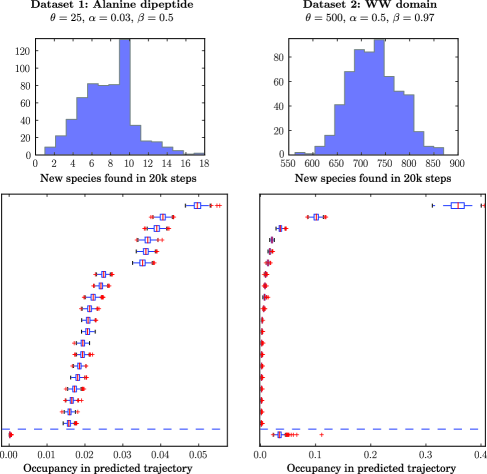
Figure 3: Posterior simulations for two molecular dynamics datasets. Top: histogram of the number of new species found in 600 simulations from the predictive distribution for $X_{n+1},\ldots,X_{n+20\mbox{,}000}$, given the data $X_{1},\ldots,X_{n}$. Bottom: box plot of the fraction of time spent at each state in these simulations. Only the twenty most populated states are shown; below the dashed line, we show the fraction of time spent at states not observed in the dataset.

conditionally sampled, the predictive simulations become straightforward with the reinforcement scheme. To provide a measure of species richness and the associated uncertainty, we histogram the number of new states discovered in our simulations in Figure 3. Only a few states are predicted to be found for dataset 1, while a large number of new states are predicted for dataset 2. This result is not surprising because the alanine dipeptide dataset has a limited number of rarely observed states, while in the WW domain data a significant number of states are observed once. This result also seems consistent with the selected values of $\theta$ and $\beta$ in these two experiments.

As previously mentioned the $(\theta,\alpha,\beta)$ scheme is a Bayesian tool for predicting any characteristic of the future trajectories $X_{n+1},\ldots,X_{n+m}$. The bottom panels in Figure 3 show confidence bands for the predicted fractions of time that will be spent at the most frequently observed states in the next 20,000 transitions. Each box in the plots refers to a single state and shows the quartiles and the 10th and 90th percentiles of the predictive distribution; states are ordered according to their mean observed frequency. We only show these occupancies for the 20 most populated states, and below the dashed line, we show the total occupancy for states that do not appear in the original data. In the WW domain example, the simulation is expected to spend between 2.5% and 5% of the time at new states.

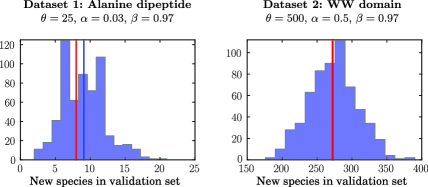
Figure 4: Bayesian predictions for the number of new species in a validation set. The histograms show the number of species found in 600 simulations from the predictive distribution for $X_{n+1},\ldots,X_{n+m}$, where $m$ is the length of the validation set and $X_{1},\ldots,X_{n}$ is the training set. The blue line shows the mean of these samples. The red line shows the actual number of new species found in the validation set. Note that in the right panel, the lines overlap due to the small separation between them.

To assess the predictive performance of the model we split each dataset into a training set and a validation set. The rationale of this procedure is identical to routinely performed cross validations for i.i.d. data. In our setting, the training and validation sets are independent portions of a homogeneous Markov chain. The first part of the procedure, which uses only the training set, includes selection of the $(\theta,\alpha,\beta)$ parameters and posterior computations. Then, we contrast Bayesian predictions to statistics of the validation set. Overall, this approach suggests that our model generates reliable predictions. Figure 4 shows histograms for the number of new species found in predictive simulations of equal length as the validation set. In each panel, the blue line is the Bayes estimate and the red line corresponds to the number of species that was actually discovered in the validation set. This approach also supports the inference reported with box plots in Figure 3. We repeated the computations for deriving the results in Figure 3 using only the training data, and considering a future trajectory equal in length to the validation data. In this case, 37 out of 42 of the true state occupancies in the validation set were contained in the 90% posterior confidence bands.

9 Discussion

We introduced a reinforced random walk with a simple predictive structure that can be represented as a mixture of reversible Markov chains. The model generalizes exchangeable and partially exchangeable sequences that have been extensively studied in the literature. Our nonparametric prior, the de Finetti measure of the $(\theta,\alpha,\beta)$ scheme, can be viewed as a distribution over weighted graphs with a countable number of vertices in a possibly uncountable space $\mathcal{X}$. As is the case for other well-known Bayesian nonparametric models such as the Dirichlet process Ferguson1973 , the hierarchical Dirichlet process Teh2006 and the infinite hidden Markov model Beal2002 , it is possible to represent our model as a function of two independent components, a species sampling sequence $(Z_{i})_{i\in\mathbb{N}}$ and a process $(T_{i})_{i\in\mathbb{N}}$ which determines the species’ locations. This property is fundamental in applications including Dirichlet process mixture models and the infinite hidden Markov model.

A natural extension of our model, not tackled here, is the definition of hidden reversible Markov models. A simple construction would consist of convolving our vertices with suitable density functions. We hope reversibility can be an advantageous assumption in relevant applications; in particular we think reversibility can be explored as a tool for the analysis of genomic data and time series from single-molecule biophysics experiments.

Appendix: Proofs from Sections 2 and 3

Proof of Proposition 2.1 Consider the latent process on $\mathcal{X}_{+}$. The transition probability from $x_{1}\in\mathcal{X}_{+}$ to $x_{2}\in\mathcal{X}_{+}$ with $g(x_{1},x_{2})>0$ is of the form $g(x_{1},x_{2})/\sum_{y\in\mathcal{X}_{+}}g(x_{1},y)$. Between successive visits to $x_{1}$, the denominator $\sum_{y\in\mathcal{X}_{+}}g(x_{1},y)$ is increased by at most $2$, and the numerator may only increase. Assume that almost surely, the process visits $x_{1}$ infinitely often. There exist $c_{2}\geq c_{1}>0$, such that if $A_{n,m}$ is the event that we do not traverse $(x_{1},x_{2})$ between the $n$th and $m$th visits to $x_{1}$,

$$p(A_{n,m})\leq\prod_{i=n}^{m-1}\biggl{[}1-\frac{c_{1}}{c_{2}+2(i-n)}\biggr{]},$$

which goes to 0 as $m\to\infty$. Therefore the edge $(x_{1},x_{2})$ is a.s. traversed infinitely often. Thus, if $x_{1}\in\mathcal{X}_{+}$ is a.s. visited infinitely often, by induction the process a.s. returns infinitely often to all visited states. Suppose a state in $\mathcal{X}$ is visited infinitely often a.s., then the process visits $\zeta$ infinitely often by the previous argument. Otherwise, the process must visit an infinite number of states in $\mathcal{X}$, and since the set of pairs $(x,y)\in\mathcal{X}^{2}$ with a positive initial weight $g(x,y)$ is a finite subset of $\mathcal{S}^{2}$, we must go through $\zeta$ an infinite number of times. We conclude that $\zeta$ is visited infinitely often a.s. and therefore the process returns to every state visited infinitely often. If $\theta>0$, then the edge $(\zeta,\zeta)$ is crossed infinitely often, and we see an infinite number of distinct states.

Proof of Proposition 3.1 For $1\leq i<n$ there is a latent variable $U_{i}\in\{a,b,c\}$ that determines in which of the three ways outlined in Figure 2 the transition $X_{i}\to X_{i+1}$ proceeded. The probability of $Z_{1}=x_{1},\ldots,Z_{n}=x_{n}$ is the sum of its joint probability with every latent sequence $U_{1}=u_{1},\ldots,U_{n-1}=u_{n-1}$. We will show that there is a one-to-one map $L$ of the latent sequences such that, letting $L(u_{1},\ldots,u_{n-1})=u^{\prime}_{1},\ldots,u^{\prime}_{n-1}$, one has

$$p(Z_{1}=x_{1},\ldots,Z_{n}=x_{n};U_{1}=u_{1},\ldots,U_{n-1}=u_{n-1})$$

(14)

$$\qquad=p\bigl{(}Z_{1}=x^{\prime}_{1},\ldots,Z_{n}=x^{\prime}_{n};U_{1}=u_{1}^{\prime},\ldots,U_{n-1}=u_{n-1}^{\prime}\bigr{)}.$$

The proposition follows from this claim. Let $t$ denote the transposition such that $d(t(x_{1},\ldots,x_{n}))=x^{\prime}_{1},\ldots,x^{\prime}_{n}$. Define $x^{\prime\prime}_{1},\ldots,x^{\prime\prime}_{n}=t(x_{1},\ldots,x_{n})$. The map $L$ is defined so that for any $u_{1},\ldots,u_{n-1}$ and $j,k<n$, satisfying

$$\mathbf{1}_{(x_{j}=x,x_{j+1}=y)}+\mathbf{1}_{(x_{j}=y,x_{j+1}=x)} > 0,$$

$$\mathbf{1}_{(x^{\prime\prime}_{k}=x,x^{\prime\prime}_{k+1}=y)}+\mathbf{1}_{(x^{\prime\prime}_{k}=y,x^{\prime\prime}_{k+1}=x)} > 0$$

for some $x$ and $y$, if

$$\sum_{i=1}^{j}\mathbf{1}_{(x_{i}=x,x_{i+1}=y)}+\mathbf{1}_{(x_{i}=y,x_{i+1}=x)}=\sum_{i=1}^{k}\mathbf{1}_{(x^{\prime\prime}_{i}=x,x^{\prime\prime}_{i+1}=y)}+\mathbf{1}_{(x^{\prime\prime}_{i}=y,x^{\prime\prime}_{i+1}=x)},$$

then $u_{j}=u^{\prime}_{k}$. Note that we can define the joint probability of $(Z_{i})_{i\leq n}$ and $(U_{i})_{i<n}$ through a reinforcement scheme identical the one defined in Section 2. Precisely, the probability of each transition and associated category is of the form

$$\frac{g(x_{i},x_{i+1})}{g(x_{i})}\mathbf{1}_{u_{i}=a},\qquad\frac{g(x_{i},\zeta)g(\zeta,x_{i+1})}{g(x_{i})g(\zeta)}\mathbf{1}_{u_{i}=b},\qquad\frac{g(x_{i},\zeta)g(\zeta,\zeta)}{g(x_{i})g(\zeta)}\mathbf{1}_{u_{i}=c},$$

where $g(x):=\sum_{y\in\mathcal{X}_{+}}g(x,y)$.

The factors $g(\zeta)$, which appear in the denominator when $U_{i}\in\{b,c\}$, are reinforced by $2\beta$ between successive visits to $\zeta$. Therefore, their product only depends on the number of mediated transitions, which is invariant under $L$. Similarly, factors $g(\zeta,\zeta)$ increase by $\alpha\beta$ between successive occurrences; their product is identical when we compute the two sides of (Appendix: Proofs from Sections 2 and 3) because the number of mediated transitions with discovery remains identical. Also, the factors $g(x)$ in the denominators increase by $2$ between successive occurrences of the same $\mathcal{X}$ state; their product is identical when we compute the two sides of (Appendix: Proofs from Sections 2 and 3) because the number of transitions out of any state $x$ (or toward $x$) remains identical. Finally, we need to prove the identity between

$$\prod_{i}\bigl{(}g(x_{i},x_{i+1})\mathbf{1}_{u_{i}=a}+g(x_{i},\zeta)g(x_{i+1},\zeta)\mathbf{1}_{u_{i}=b}+g(x_{i},\zeta)\mathbf{1}_{u_{i}=c}\bigr{)}$$ (15)

and

$$\prod_{i}\bigl{(}g\bigl{(}x^{\prime}_{i},x^{\prime}_{i+1}\bigr{)}\mathbf{1}_{u^{\prime}_{i}=a}+g\bigl{(}x^{\prime}_{i},\zeta\bigr{)}g\bigl{(}x^{\prime}_{i+1},\zeta\bigr{)}\mathbf{1}_{u^{\prime}_{i}=b}+g\bigl{(}x^{\prime}_{i},\zeta\bigr{)}\mathbf{1}_{u^{\prime}_{i}=c}\bigr{)}.$$ (16)

The identity between (15) and (16) follows by combining the definitions of $d$ and $L$ with the reinforcement mechanism. Specifically, the factors $g(x,\zeta)$ and $g(x^{\prime},\zeta)$ are increased by $\beta$ between successive occurrences. Since $g(x,\zeta)$ appears as many times in the left-hand side of (Appendix: Proofs from Sections 2 and 3) as $g(x^{\prime},\zeta)$ does in the right-hand side of (Appendix: Proofs from Sections 2 and 3), the product of these factors is identical in each case. The remaining factors $g(x,y)$ may increase by different amounts between successive occurrences. Their product is a function of the subsequence of $U_{1},\ldots,U_{n-1}$ with indices $\{1\leq i<n\dvtx\{Z_{i},Z_{i+1}\}=\{x,y\}\}$. By the definition of $L$, this subsequence is the same in the left and right-hand sides of (Appendix: Proofs from Sections 2 and 3), which completes the proof of our claim.

Proof of Proposition 3.2 Let $(X_{i}^{\prime\prime})_{i\in\mathbb{N}}$ be a $(\theta,\alpha,\beta)$ scheme. The process $(X_{i}^{\prime\prime})_{i\in\mathbb{N}}$ returns to $X_{1}^{\prime\prime}$ infinitely often a.s. Let $h_{i}$ be the $i$th $X_{1}^{\prime\prime}$-block. Define $(X_{i})_{i\in\mathbb{N}}:=(h_{1},h_{3},h_{5},\ldots)$ and $(X^{\prime}_{i})_{i\in\mathbb{N}}:=(h_{2},h_{4},h_{6},\ldots)$. Proposi-tion 3.1 implies $(X_{i})_{i\in\mathbb{N}}\stackrel{{\scriptstyle\mathrm{d}}}{{=}}(X^{\prime}_{i})_{i\in\mathbb{N}}\stackrel{{\scriptstyle\mathrm{d}}}{{=}}(X^{\prime\prime}_{i})_{i\in\mathbb{N}}$. Let $\operatorname{Fin}(x)$ be the last element of a vector $x$. Define

$$W_{i}:=\lim_{m\rightarrow\infty}\operatorname{Fin}\bigl{(}d\bigl{(}X^{\prime}_{1},X^{\prime}_{2},\ldots,X^{\prime}_{m},X_{1},X_{2},\ldots,X_{i}\bigr{)}\bigr{)}.$$

This limit exists a.s. because $X_{i}$ is recurrent in $(X^{\prime\prime}_{j})_{j\in\mathbb{N}}$; therefore, the sequence of blocks that form $(X^{\prime}_{j})_{j\in\mathbb{N}}$ is conditionally i.i.d. from a distribution which a.s. assigns positive probability to blocks containing $X_{i}$, which implies $(X^{\prime}_{j})_{j\in\mathbb{N}}$ visits $X_{i}$ after a finite time a.s., at which point the limit settles.

In Lemma .1 we show that $(W_{i})_{i\in\mathbb{N}}$ is Markov exchangeable and recurrent. Therefore, by de Finetti’s theorem for Markov chains (3.1), it is a mixture of Markov chains. Finally, by Lemma .2, we obtain the representation claimed in the proposition.

Lemma .1

Without loss of generality, let $\mathcal{X}=(0,1)$. The process $(W_{i})_{i\in\mathbb{N}}$ is Markov exchangeable and returns to every state in $\mathcal{S}\sqcup\mathbb{N}$ infinitely often a.s.

The recurrence of $(Z_{i})_{i\in\mathbb{N}}$, which is a consequence of Proposition 2.1, implies the recurrence of $(W_{i})_{i\in\mathbb{N}}$. Thus, we have left to show Markov exchangeability.

The sequence $W_{1},\ldots,W_{n}$ can be mapped through $d$ to $Z_{1},\ldots,Z_{n}$, which is a species sampling sequence for the $(\theta,\alpha,\beta)$ scheme. Take any sequence $w_{1},\ldots,w_{n}$ and let $z_{1},\ldots,z_{n}:=d(w_{1},\ldots,w_{n})$. We have

$$p(W_{1}=w_{1},\ldots,W_{n}=w_{n})$$

$$\qquad=p(Z_{1}=z_{1},\ldots,Z_{n}=z_{n})$$ (17)

$$\qquad\quad{}\times p(W_{1}=w_{1},\ldots,W_{n}=w_{n}|Z_{1}=z_{1},\ldots,Z_{n}=z_{n}).$$

Consider any pair of sequences $w_{1},\ldots,w_{n}$ and $w^{\prime}_{1},\ldots,w^{\prime}_{n}$ related by a transposition of two blocks with identical initial and final states. Proposition 3.1 implies

$$p\bigl{(}(Z_{1},\ldots,Z_{n})=d(w_{1},\ldots,w_{n})\bigr{)}=p\bigl{(}(Z_{1},\ldots,Z_{n})=d\bigl{(}w^{\prime}_{1},\ldots,w^{\prime}_{n}\bigr{)}\bigr{)}.$$

We have left to show that the second factor on the right-hand side of (Appendix: Proofs from Sections 2 and 3) is identical for $w_{1},\ldots,w_{n}$ and $w^{\prime}_{1},\ldots,w^{\prime}_{n}$. The identity of the conditional distribution of $(X_{i}^{\prime})_{i\in\mathbb{N}}$ given $(Z_{1},\ldots,Z_{n})$ equal to $d(w_{1},\ldots,w_{n})$ or equal to $d(w^{\prime}_{1},\ldots,w^{\prime}_{n})$ proves the lemma.

Lemma .2

The process $(T_{W_{i}}\mathbf{1}_{W_{i}\notin\mathcal{S}}+W_{i}\mathbf{1}_{W_{i}\in\mathcal{S}})_{i\in\mathbb{N}}$ has the same distribution as $(X_{i})_{i\in\mathbb{N}}$.

By definition $(X_{i})_{i\in\mathbb{N}}\stackrel{{\scriptstyle\mathrm{d}}}{{=}}(T_{Z_{i}}\mathbf{1}_{Z_{i}\notin\mathcal{S}}+Z_{i}\mathbf{1}_{Z_{i}\in\mathcal{S}})_{i\in\mathbb{N}}$. Note that$(T_{i})_{i\in\mathbb{N}}$ is an i.i.d. sequence, independent from $(Z_{i})_{i\in\mathbb{N}}$, and $d((W_{i})_{i\in\mathbb{N}})=(Z_{i})_{i\in\mathbb{N}}$. These facts imply that $(T_{W_{i}}\mathbf{1}_{W_{i}\notin\mathcal{S}}+W_{i}\mathbf{1}_{W_{i}\in\mathcal{S}})_{i\in\mathbb{N}}\stackrel{{\scriptstyle\mathrm{d}}}{{=}}(T_{Z_{i}}\mathbf{1}_{Z_{i}\notin\mathcal{S}}+Z_{i}\mathbf{1}_{Z_{i}\in\mathcal{S}})_{i\in\mathbb{N}}$.

Proof of Proposition 3.3 Let $h_{1},h_{2},\ldots$ be the $X_{1}$-blocks of the $(\theta,\alpha,\beta)$ scheme. Consider a map $s$ on the $X_{1}$-blocks’ space; if $a=(a_{1},\ldots,a_{m})$, then $s(a)=(a_{1},a_{m},a_{m-1},\ldots,a_{2})$. We can observe, following the same arguments used for proving Proposition 3.1, that for any $X_{1}$-block $a$ and any integer $n$,

$$p(h_{1}=a,h_{2},\ldots,h_{n})=p\bigl{(}h_{1}=s(a),h_{2},\ldots,h_{n}\bigr{)}.$$

Let $F$ be a random measure distributed according to the de Finetti measure of the $X_{1}$-blocks. The above expression and the equality

$$\lim_{n\to\infty}p(h_{1}\in A|h_{2},\ldots,h_{n})\stackrel{{\scriptstyle\mathrm{a.s.}}}{{=}}F(A),$$

where $A$ is a generic measurable set, imply that a.s. the distance in total variation between $F$ and $F\circ s$ is null.

References

- (1) {barticle}[mr] \bauthor\bsnmBacallado, \bfnmSergio\binitsS. (\byear2011). \btitleBayesian analysis of variable-order, reversible Markov chains. \bjournalAnn. Statist. \bvolume39 \bpages838–864. \biddoi=10.1214/10-AOS857, issn=0090-5364, mr=2816340 \bptokimsref \endbibitem
- (2) {bmisc}[author] \bauthor\bsnmBacallado, \bfnmS.\binitsS., \bauthor\bsnmFavaro, \bfnmS.\binitsS. and \bauthor\bsnmTrippa, \bfnmL.\binitsL. (\byear2013). \btitleSupplement to “Bayesian nonparametric analysis of reversible Markov chains.” DOI:\doiurl10.1214/13-AOS1102SUPP. \bptokimsref \endbibitem
- (3) {barticle}[author] \bauthor\bsnmBeal, \bfnmM. J.\binitsM. J., \bauthor\bsnmGhahramani, \bfnmZ.\binitsZ. and \bauthor\bsnmRasmussen, \bfnmC. E.\binitsC. E. (\byear2002). \btitleThe infinite hidden Markov model. \bjournalAdv. Neural Inf. Process. Syst. \bvolume14 \bpages577–584. \bptokimsref \endbibitem
- (4) {barticle}[mr] \bauthor\bsnmBlackwell, \bfnmDavid\binitsD. and \bauthor\bsnmMacQueen, \bfnmJames B.\binitsJ. B. (\byear1973). \btitleFerguson distributions via Pólya urn schemes. \bjournalAnn. Statist. \bvolume1 \bpages353–355. \bidissn=0090-5364, mr=0362614 \bptokimsref \endbibitem
- (5) {barticle}[author] \bauthor\bsnmBunge, \bfnmJ.\binitsJ. and \bauthor\bsnmFitzpatrick, \bfnmM.\binitsM. (\byear1993). \btitleEstimating the number of species: A review. \bjournalJ. Amer. Statist. Assoc. \bvolume88 \bpages364–373. \bptokimsref \endbibitem
- (6) {bbook}[mr] \bauthor\bsnmComtet, \bfnmLouis\binitsL. (\byear1974). \btitleAdvanced Combinatorics: The Art of Finite and Infinite Expansions, \beditionenlarged ed. \bpublisherReidel, \blocationDordrecht. \bidmr=0460128 \bptokimsref \endbibitem
- (7) {binproceedings}[author] \bauthor\bsnmDiaconis, \bfnmP.\binitsP. (\byear1988). \btitleRecent progress on de Finetti notions of exchangeability. In \bbooktitleBayesian Statistics 3 (\beditor\bfnmJ. M.\binitsJ. M. \bsnmBernardo, \beditor\bfnmM. H.\binitsM. H. \bsnmDeGroot, \beditor\bfnmD. V.\binitsD. V. \bsnmLindley and \beditor\bfnmA. F. M.\binitsA. F. M. \bsnmSmith, eds.) \bpages111–125. \bpublisherOxford Univ. Press, \blocationNew York. \bptokimsref \endbibitem
- (8) {barticle}[mr] \bauthor\bsnmDiaconis, \bfnmP.\binitsP. and \bauthor\bsnmFreedman, \bfnmD.\binitsD. (\byear1980). \btitlede Finetti’s theorem for Markov chains. \bjournalAnn. Probab. \bvolume8 \bpages115–130. \bidissn=0091-1798, mr=0556418 \bptokimsref \endbibitem
- (9) {barticle}[mr] \bauthor\bsnmDiaconis, \bfnmPersi\binitsP. and \bauthor\bsnmRolles, \bfnmSilke W. W.\binitsS. W. W. (\byear2006). \btitleBayesian analysis for reversible Markov chains. \bjournalAnn. Statist. \bvolume34 \bpages1270–1292. \biddoi=10.1214/009053606000000290, issn=0090-5364, mr=2278358 \bptokimsref \endbibitem
- (10) {bbook}[mr] \bauthor\bsnmEngen, \bfnmS.\binitsS. (\byear1978). \btitleStochastic Abundance Models: With Emphasis on Biological Communities and Species Diversity. \bpublisherChapman & Hall, \blocationLondon. \bidmr=0515721 \bptokimsref \endbibitem
- (11) {barticle}[mr] \bauthor\bsnmFavaro, \bfnmStefano\binitsS., \bauthor\bsnmLijoi, \bfnmAntonio\binitsA., \bauthor\bsnmMena, \bfnmRamsés H.\binitsR. H. and \bauthor\bsnmPrünster, \bfnmIgor\binitsI. (\byear2009). \btitleBayesian non-parametric inference for species variety with a two-parameter Poisson–Dirichlet process prior. \bjournalJ. R. Stat. Soc. Ser. B Stat. Methodol. \bvolume71 \bpages993–1008. \biddoi=10.1111/j.1467-9868.2009.00717.x, issn=1369-7412, mr=2750254 \bptokimsref \endbibitem
- (12) {barticle}[mr] \bauthor\bsnmFerguson, \bfnmThomas S.\binitsT. S. (\byear1973). \btitleA Bayesian analysis of some nonparametric problems. \bjournalAnn. Statist. \bvolume1 \bpages209–230. \bidissn=0090-5364, mr=0350949 \bptokimsref \endbibitem
- (13) {barticle}[mr] \bauthor\bsnmFortini, \bfnmS.\binitsS. and \bauthor\bsnmPetrone, \bfnmS.\binitsS. (\byear2012). \btitleHierarchical reinforced urn processes. \bjournalStatist. Probab. Lett. \bvolume82 \bpages1521–1529. \biddoi=10.1016/j.spl.2012.04.012, issn=0167-7152, mr=2930656 \bptokimsref \endbibitem
- (14) {barticle}[mr] \bauthor\bsnmIshwaran, \bfnmHemant\binitsH. and \bauthor\bsnmJames, \bfnmLancelot F.\binitsL. F. (\byear2001). \btitleGibbs sampling methods for stick-breaking priors. \bjournalJ. Amer. Statist. Assoc. \bvolume96 \bpages161–173. \biddoi=10.1198/016214501750332758, issn=0162-1459, mr=1952729 \bptokimsref \endbibitem
- (15) {bincollection}[mr] \bauthor\bsnmKeane, \bfnmM. S.\binitsM. S. and \bauthor\bsnmRolles, \bfnmS. W. W.\binitsS. W. W. (\byear2000). \btitleEdge-reinforced random walk on finite graphs. In \bbooktitleInfinite Dimensional Stochastic Analysis (Amsterdam, 1999). \bseriesVerh. Afd. Natuurkd. 1. Reeks. K. Ned. Akad. Wet. \bvolume52 \bpages217–234. \bpublisherR. Neth. Acad. Arts Sci., \blocationAmsterdam. \bidmr=1832379 \bptokimsref \endbibitem
- (16) {barticle}[mr] \bauthor\bsnmLijoi, \bfnmAntonio\binitsA., \bauthor\bsnmMena, \bfnmRamsés H.\binitsR. H. and \bauthor\bsnmPrünster, \bfnmIgor\binitsI. (\byear2007). \btitleBayesian nonparametric estimation of the probability of discovering new species. \bjournalBiometrika \bvolume94 \bpages769–786. \biddoi=10.1093/biomet/asm061, issn=0006-3444, mr=2416792 \bptokimsref \endbibitem
- (17) {barticle}[pbm] \bauthor\bsnmLijoi, \bfnmAntonio\binitsA., \bauthor\bsnmMena, \bfnmRamsés H.\binitsR. H. and \bauthor\bsnmPrünster, \bfnmIgor\binitsI. (\byear2007). \btitleA Bayesian nonparametric method for prediction in EST analysis. \bjournalBMC Bioinformatics \bvolume8 \bpages339–349. \biddoi=10.1186/1471-2105-8-339, issn=1471-2105, pii=1471-2105-8-339, pmcid=2220008, pmid=17868445 \bptokimsref \endbibitem
- (18) {barticle}[mr] \bauthor\bsnmMerkl, \bfnmFranz\binitsF. and \bauthor\bsnmRolles, \bfnmSilke W. W.\binitsS. W. W. (\byear2009). \btitleRecurrence of edge-reinforced random walk on a two-dimensional graph. \bjournalAnn. Probab. \bvolume37 \bpages1679–1714. \biddoi=10.1214/08-AOP446, issn=0091-1798, mr=2561431 \bptokimsref \endbibitem
- (19) {barticle}[pbm] \bauthor\bsnmPande, \bfnmVijay S.\binitsV. S., \bauthor\bsnmBeauchamp, \bfnmKyle\binitsK. and \bauthor\bsnmBowman, \bfnmGregory R.\binitsG. R. (\byear2010). \btitleEverything you wanted to know about Markov State Models but were afraid to ask. \bjournalMethods \bvolume52 \bpages99–105. \biddoi=10.1016/j.ymeth.2010.06.002, issn=1095-9130, mid=NIHMS218238, pii=S1046-2023(10)00156-8, pmcid=2933958, pmid=20570730 \bptokimsref \endbibitem
- (20) {bincollection}[mr] \bauthor\bsnmPitman, \bfnmJim\binitsJ. (\byear1996). \btitleSome developments of the Blackwell–MacQueen urn scheme. In \bbooktitleStatistics, Probability and Game Theory. \bseriesInstitute of Mathematical Statistics Lecture Notes—Monograph Series (\beditor\bfnmT. S.\binitsT. S. \bsnmFerguson, \beditor\bfnmL. S.\binitsL. S. \bsnmShapley and \beditor\bfnmJ. B.\binitsJ. B. \bsnmMacQueen, eds.) \bvolume30 \bpages245–267. \bpublisherIMS, \blocationHayward, CA. \biddoi=10.1214/lnms/1215453576, mr=1481784 \bptokimsref \endbibitem
- (21) {barticle}[mr] \bauthor\bsnmPitman, \bfnmJim\binitsJ. and \bauthor\bsnmYor, \bfnmMarc\binitsM. (\byear1997). \btitleThe two-parameter Poisson–Dirichlet distribution derived from a stable subordinator. \bjournalAnn. Probab. \bvolume25 \bpages855–900. \biddoi=10.1214/aop/1024404422, issn=0091-1798, mr=1434129 \bptokimsref \endbibitem
- (22) {binproceedings}[mr] \bauthor\bsnmPropp, \bfnmJames Gary\binitsJ. G. and \bauthor\bsnmWilson, \bfnmDavid Bruce\binitsD. B. (\byear1996). \btitleExact sampling with coupled Markov chains and applications to statistical mechanics. In \bbooktitleProceedings of the Seventh International Conference on Random Structures and Algorithms (Atlanta, GA, 1995) 9 \bpages223–252. \bpublisherWiley, \blocationNew York. \biddoi=10.1002/(SICI)1098-2418(199608/09)9:1/2<223::AID-RSA14>3.3.CO;2-R, issn=1042-9832, mr=1611693 \bptokimsref \endbibitem
- (23) {barticle}[mr] \bauthor\bsnmRolles, \bfnmSilke W. W.\binitsS. W. W. (\byear2003). \btitleHow edge-reinforced random walk arises naturally. \bjournalProbab. Theory Related Fields \bvolume126 \bpages243–260. \biddoi=10.1007/s00440-003-0260-8, issn=0178-8051, mr=1990056 \bptokimsref \endbibitem
- (24) {barticle}[pbm] \bauthor\bsnmShaw, \bfnmDavid E.\binitsD. E. (\byear2010). \btitleAtomic-level characterization of the structural dynamics of proteins. \bjournalScience \bvolume330 \bpages341–346. \biddoi=10.1126/science.1187409, issn=1095-9203, pii=330/6002/341, pmid=20947758 \bptokimsref \endbibitem
- (25) {bincollection}[mr] \bauthor\bsnmTeh, \bfnmYee Whye\binitsY. W. and \bauthor\bsnmJordan, \bfnmMichael I.\binitsM. I. (\byear2010). \btitleHierarchical Bayesian nonparametric models with applications. In \bbooktitleBayesian Nonparametrics \bpages158–207. \bpublisherCambridge Univ. Press, \blocationCambridge. \bidmr=2730663 \bptokimsref \endbibitem
- (26) {barticle}[mr] \bauthor\bsnmTeh, \bfnmYee Whye\binitsY. W., \bauthor\bsnmJordan, \bfnmMichael I.\binitsM. I., \bauthor\bsnmBeal, \bfnmMatthew J.\binitsM. J. and \bauthor\bsnmBlei, \bfnmDavid M.\binitsD. M. (\byear2006). \btitleHierarchical Dirichlet processes. \bjournalJ. Amer. Statist. Assoc. \bvolume101 \bpages1566–1581. \biddoi=10.1198/016214506000000302, issn=0162-1459, mr=2279480 \bptokimsref \endbibitem
- (27) {barticle}[mr] \bauthor\bsnmZabell, \bfnmSandy L.\binitsS. L. (\byear1982). \btitleW. E. Johnson’s “sufficientness” postulate. \bjournalAnn. Statist. \bvolume10 \bpages1090–1099 (1 plate). \bidissn=0090-5364, mr=0673645 \bptokimsref \endbibitem
- (28) {bincollection}[mr] \bauthor\bsnmZabell, \bfnmS. L.\binitsS. L. (\byear2005). \btitleThe continuum of inductive methods revisited. In \bbooktitleSymmetry and its Discontents: Essays on the History of Inductive Probability. \bpublisherCambridge Univ. Press, \blocationNew York. \bptokimsref \endbibitem