Analytical Treatment of Coherent Excitation Transfer in FMO Complex

Abstract

We suggest a new method of studying coherence in finite level systems coupled to the environment and use it for the Hamiltonian that has been used to describe the light-harvesting pigment-protein complex. The method works with the adiabatic states and transforms the Hamiltonian to a form in which the terms responsible for decoherence and population relaxation are separated out. Decoherence is then accounted for non-perturbatively, and population relaxation using a Markovian master equation. Analytical results can be obtained for the seven level system and the calculations are very simple for systems with more levels. We apply the treatment to the seven level system and the results are in excellent agreement with the exact numerical results of Nalbach et al (P. Nalbach, D. Braun, and M. Thorwart, Physical Review E, 84, 041926 (2011)). Our approach is able to account for decoherence and population relaxation separately. It is found that decoherence only causes damping of oscillations, and does not lead to transfer to the reaction centre. Population relaxation is necessary for efficient transfer to the reaction centre, in agreement with earlier findings. Our results show that the transformation to the adiabatic basis followed by a Redfield type of approach leads to results in good agreement with exact simulation.

I Introduction

Photosynthesis by plants is one of the most ubiquitous phenomena on earth. It involves the creation of excitations by absorption of photons and the transfer of this excitation to the reaction centre where the crucial step in photosynthesis, namely the transfer of an electron takes place. This transfer of energy from the absorption site to the reaction site is called light harvesting and is highly efficient with more than 95% of the absorbed energy being transferred to the reaction centre. One expects this transfer to be incoherent classical hopping (Förster transfer) from one chromophore to the next. The reason for this is that the chromophores do not exist isolated. They are surrounded by a protein scaffold and solvent molecules. Consequently the excitation which might be considered as a wave encompassing more than a single site/chromophore is then continuously measured by the surroundings, viz., the proteins and the solvent. Therefore the superposition is expected to be rapidly destroyed (within $\backsim 10\ fs$) resulting in the localization of the excitation at a particular site. The excitation now exhibits particle-like behavior and the transfer takes place through a series of independent hops. However, lately there have been some very interesting experiments reported by Fleming and coworkers Brixner et al. (2005); Engel et al. (2007); Read et al. (2007) which observe coherent excitation energy transfer over a considerable period of time. It should be noted that there have also been studies in which role of coherence was investigated and found to be important in determining the rate of energy transfer Leegwater et al. (1997); Kuehn and Sundstroem (1997); Renger and May (1998).

The FMO complex Fenna and Matthews (1975); Li et al. (1997); Camara-Artigas et al. (2003) or the Fenna-Matthews-Olson complex is found in green sulfur bacteria. It forms a kind of bridge between the peripheral chlorosome antenna and the reaction centre and is endowed with the important task of transferring the excitation energy from the antenna to the reaction centre. It is essentially a trimer of identical subunits, each comprising seven bacteriocholophyll a molecules. Recent 2D Electronic spectroscopy studies observe coherence for as long as $660$ fs at $77$ K Engel et al. (2007) and $300$ fs at $277$ K Panitchayangkoon et al. (2010). The observations are very surprising for one would expect rapid decoherence for a system interacting so profusely with its environment Prezhdo and Rossky (1998); Gilmore and McKenzie (2006, 2008); Nalbach et al. (2011); Rebentrost et al. (2009, 2009); Abramavicius and Mukamel (2010); Singh (2012). Decoherence refers to the loss of coherence, caused by the quantum nature of the surroundings and can be avoided only by sufficiently isolating the system, and by keeping the temperatures low. However, the above experiments suggest that quantum coherence can be maintained even in wet and hot physiological systems and this has led to a great deal of interest and to the emergence of what may be referred to as Quantum Biology Ball (2011); Lloyd (2011).

Theoretical studies for the same were conducted by Fleming and coworkers. They formulated a treatment where a quantum dynamical equation is proposed which considers the reorganization dynamics of the surroundings non-perturbatively in a hierarchical expansion. These predicted the survival of coherence at room temperature Ishizaki and Fleming (2009, 2009) as well. There were also similar conclusions from the theoretical studies by other groups Mohseni et al. (2008); Caruso et al. (2009); Olaya-Castro and Scholes (2011). Guzik et al. Mohseni et al. (2008) developed continuous quantum walks in the Liouville space. Their studies suggested that the interplay between the coherent dynamics of the system and the dissipative influence of the environment assists in more efficient transport of the excitation compared to the case where the environment is considered absent. Independent studies by Plenio et al. Caruso et al. (2009) also suggested quantum transport assisted by noise due to environment. While these are approximate results, in a very interesting paper, exact numerical studies have been performed recently for the FMO complex by Nalbach et al. Nalbach et al. (2011). It should also be mentioned that there have also been some studies which ruled out coherence. These were atomistic simulations by Kleinekathöfer Olbrich et al. (2011) $\mathit{et}$ $\mathit{al}$., which sought to calculate the spectral densities for the FMO trimer. The studies proposed that the electron-phonon coupling was much stronger than what was considered previously. A stronger coupling with the environment would imply faster and more efficient destruction of coherence. Path integral Monte Carlo simulations by the same group M$\ddot{u}$hlbacher and Kleinekathofer (2012) suggested that coherence would not be retained with the initial excitation put on a specific chromophore. However it could survive if the initial excitation was delocalised. The point worth noting here is that all the above methods employed numerical methods or simulations and were computationally quite expensive. Also, population relaxation and decoherence resulted from the same term in the Hamiltonian. We also note that the related problem of coherence in the spin boson problem has been a subject of a large amount of literature Weiss (2008); Orth et al. (2010, 2010).

At this point, we emphasize that the definition of decoherence we follow is the one used by Schlosshauer in his book on decoherence Schlosshauer (2007). We quote from the book: “We consistently reserve the term decoherence to describe the consequences of (usually in practice irreversible) quantum entanglement with some environment, in agreement with the historically established meaning and the vast body of literature on environmental decoherence….. Thus decoherence should be understood as a distinctly quantum-mechanical effect with no classical analog.” As a result, we consider population relaxation to be distinct from decoherence, unlike many other authors.

In this paper we propose an analytical approach for treating such coherences. The main advantage of the treatment is that the evaluation is numerically inexpensive, and it can be easily performed for the FMO protein (seven-level system). Further it can be easily extended to systems with larger number of states unlike the existing approaches which are computationally expensive and hence difficult to apply to systems with large number of states. A comparison of results obtained with our method with the exact numerical studies by Nalbach Nalbach et al. (2011) has also been provided. The agreement between the two is excellent. Our method uses the adiabatic basis of the Hamiltonian and as we show below, we can treat the population relaxation and decoherence independently and hence more efficiently. In Section II, we introduce the generalised electronic Hamiltonian that is commonly used and transform it to the adiabatic basis in Section III. Section IV deals with the reduced density matrix of the system which would give us independent expressions for population relaxation and decoherence. In Section V, the FMO Hamiltonian is introduced and analytical expressions are given for the reduced density matrix elements at a time $t.$ Section VI contains the results and discussions. While almost all our results are concerned with a situation in which there are no correlations between the phonon baths for the different chromophores, in Section VII we give a brief discussion of how spatial correlations affect the energy transfer. We summarize our results in Section VIII.

II The Hamiltonian

The Hamiltonian that is commonly used has the minimum number of terms, that are required to account for the phenomena. The FMO complex has a finite number ($N=7$) of bacteriochlorophyll a molecules. Each bacteriochlorophyll a can be in the excited state or the ground state. The separation between these two is large ($\approx 12500\;cm^{-1}$) and the two states are only radiatively coupled. Environmental tuning makes the excitation energies on different bacteriochlorophylls different, though by small amounts, thus helping the flow of energy. The energy values relative to the lowest element are given by the diagonal elements of the matrix in Eq. (40). The dipolar coupling between the bacteriochlorophylls is responsible for the transfer of excitation from one bacteriochlorophyll to the next. Its magnitude is typically less than $100\;cm^{-1}$. We describe the electronic part of the Hamiltonian by

$$H_{el}=\sum_{j}\epsilon_{j}|j\rangle\langle j|+\sum_{i,j}(V_{ij}|i\rangle\langle j|+V_{ji}|j\rangle\langle i|),$$ (1)

where $|j\rangle$ with $j=1,2...N$ denotes the state in which the excitation is on the $j^{th}$ bacteriochlorophyll a molecule. $\epsilon_{j}$ is the energy appropriate for this state. Note that in Eq. (40) the diagonal matrix element for the excitation having the lowest energy of value $12210\ cm^{-1}$ is taken as the reference. When the excitation is on the $j^{th}$ site, it interacts with its surroundings (the nuclear degrees of freedom) and this is responsible for decoherence and relaxation within these states. The model used for surroundings is a collection of harmonic oscillators. On the $j^{th}$ bacteriochlorophyll site, the coupling is to a set of phonons represented by

$$H_{ph,j}=\frac{1}{2}\sum_{k}(\frac{\hat{p}_{jk}^{2}}{m_{jk}}+m_{jk}\omega_{jk}^{2}q_{jk}^{2}),$$ (2)

$q_{jk}$ being the position of the $k^{th}$ harmonic oscillator associated with the $j^{th}$ site. It has a mass $m_{jk}$ and frequency $\omega_{jk}$. $p_{jk}$ is the momentum operator. Thus the total phonon system has the Hamiltonian

$$H_{ph}=\sum_{j}H_{ph,j}.$$ (3)

The presence of the excitation on the $j^{th}$ site causes modification of the phonon Hamiltonian. The excitation causes a shift in the equilibrium positions of the phonons. This is accounted for by $Q_{j}$ in equations (4) and (5). Eq. (5) implies that this term may also be thought of as a shift of the energy of the $j^{th}$ excited state by the fluctuations of the phonons.

$$Q_{j}=\sum_{k}m_{jk}\nu_{jk}q_{jk},$$ (4)

with

$$H_{el-ph}=\sum_{j}Q_{j}|j\rangle\langle j|.$$ (5)

Thus the total Hamiltonian is

$$H=H_{el}+H_{ph}+H_{el-ph}.$$ (6)

Interestingly, with this type of coupling to the phonon system, the time evolution of the excitation is determined just by the spectral densities for each site, defined by Weiss (2008)

$$J_{j}(\omega)=\sum_{k}\frac{m_{jk}\nu_{jk}^{2}}{2\omega_{jk}}\delta(\omega-\omega_{jk}).$$ (7)

When the $j^{th}$ site is excited, the excitation would cause a shift in the equilibrium positions of all the harmonic oscillators for this site. The displacement of the $k^{th}$ oscillator is $\nu_{jk}/\omega_{jk}^{2}$ costing an energy $\frac{m_{jk}\nu_{jk}^{2}}{2\omega_{jk}^{2}}$. Sum of this for all the oscillators is denoted by $\lambda_{j}=\frac{1}{2}\sum_{k}\frac{m_{jk}\nu_{jk}^{2}}{\omega_{jk}^{2}}$ and is called the reorganization energy for that site. It may be written as

$$\lambda_{j}=\int_{0}^{\infty}d\omega J_{j}(\omega)/\omega.$$ (8)

The Hamiltonian has two competing sets of parameters which affect the energy transport in opposite ways. The first are the off-diagonal exciton-exciton coupling $V_{ij}$ responsible for energy transfer and the other being the exciton-phonon coupling, measured by the reorganisation energy $\lambda_{j}$. If $|V_{ij}|\ \gg\ \lambda_{j}$, we essentially have delocalised eigenstates instead of energy being localised to a particular site and the energy transfer is quantum mechanical and coherent. One has incoherent, Förster like transfer in the opposite limit where $|V_{ij}|\ \ll\ \lambda_{j}$. The fluctuations of the phonons associated with different sites are likely to be independent, and there is some evidence from simulations M$\ddot{u}$hlbacher and Kleinekathofer (2012) showing this to be the case. However, it has also been suggested that the correlations are important and models in which there are correlations have been investigated. The correlations can be accounted for by taking Sarovar et al. (2011):

$$\langle Q_{i}(t)Q_{j}(0)\rangle=C_{ij}\langle Q_{i}(t)Q_{i}(0)\rangle.$$ (9)

In the above equation, $C$ is the correlation matrix with the matrix element $C_{ij}$ denoting the correlation among the chromophores i and j. Obviously, $C_{ii}=1$. In most of the following, except in Section VIII, we have assumed that $C_{ij}=\delta_{ij}$ and $J_{j}(\omega)=J(\omega)$ for all $j$.

However, if $\lambda_{j}\ \gg\ |V_{ij}|$, the strong interaction with the environment makes it difficult for a delocalised state to survive. Consequently one would expect classical incoherent particle-like hopping of the excitation from one site to the other. There would also be an intermediate regime where $|V_{ij}|$ and $\lambda_{j}$ are comparable, and this is the case of the FMO complex.

In the usual approaches, for the intermediate regime conditions, one would take $H_{el-ph}$ as a perturbation Ishizaki and Fleming (2009) and then derive a master equation for the time development of the reduced density matrix, which then is solved approximately using different techniques. It is important to realize that in this type of approach, the same term ($H_{el-ph})$ causes both decoherence and population relaxation. One would then resort to some approximate way of handling the perturbation, involving truncating at some order in $Q_{j}$s. Our approach here follows a different route. We use an approach usual in the theory of non-adiabaticity effects in chemical reactions Baer (2006). We re-express the Hamiltonian in terms of the adiabatic states. In such a representation, accounting for decoherence becomes easy as a part of the adiabatic Hamiltonian is responsible for major component of the decoherence and the non-adiabatic coupling causes population relaxation. Thus the two important effects of $H_{el-ph}$ viz., decoherence and population relaxation are separated out (at the lowest order) and can be accounted for separately, in a natural fashion. Once this separation is done, the calculation proceeds in a fashion similar to references Zhang et al. (1998); Yang and Fleming (2002). In the next section, we give an outline of the approach.

III The adiabatic basis and the mapping $T(\mathbf{Q})$

It is convenient to use the notation $\mathbf{Q}=(Q_{1},Q_{2}...)$. The survival of coherences for long times implies that there is considerable delocalization even in presence of the environment. Therefore, it is natural to expect that the adiabatic eigenfunctions of the Hamiltonian

$$H_{ad}(\mathbf{Q})=H_{el}+H_{el-ph},$$ (10)

would be the best starting point to describe dynamics. Therefore, we wish to express the total Hamiltonian of Eq. (6) in terms of the eigenfunctions $|m(\mathbf{Q})\rangle$, with $m=1,2....N$. They obey the equation

$$H_{ad}(\mathbf{Q})|m(\mathbf{Q})\rangle=\varepsilon_{m}(\mathbf{Q})|m(\mathbf{Q})\rangle.$$ (11)

$|m(\mathbf{Q})\rangle$ are obviously linear combinations of $|j\rangle$ with the coefficients dependent on $\mathbf{Q}$. It is also convenient to introduce creation and annihilation operators for these states as $c_{m}^{\dagger}(\mathbf{Q})$ and $c_{m}(\mathbf{Q})$ (the operators have the anticommutator $\{c_{m}^{\dagger}(\mathbf{Q}),c_{n}(\mathbf{Q})\}=\delta_{mn}$). We can then write the total Hamiltonian as

$$H=\sum_{m}\varepsilon_{m}(\mathbf{Q})c_{m}^{\dagger}(\mathbf{Q})c_{m}(\mathbf{Q})+H_{ph}.$$ (12)

This Hamiltonian has the problem that $c_{m}^{\dagger}(\mathbf{Q})$ does not commute with $H_{ph}$. It would be better if the Hamiltonian is expressed in terms of $c_{m}^{\dagger}(\mathbf{Q}=0)$ as they will commute with $H_{ph}$. Note that $\mathbf{Q}=\mathbf{0}$ is the equilibrium value of $\mathbf{Q}$. Hence we introduce a unitary transformation which maps $|m(\mathbf{Q})\rangle$ to $|m(\mathbf{Q=0})\rangle$ as $|m(\mathbf{Q})\rangle=T(\mathbf{Q})|m>$. To simplify the appearence of the equations, we use the notation $|m\rangle$ for $|m(\mathbf{Q}=\mathbf{0})>$ and write the corresponding operator as $c_{m}^{\dagger}$. Obviously, $c_{m}^{\dagger}=T^{\dagger}(\mathbf{Q})c_{m}^{\dagger}(\mathbf{Q})T(\mathbf{Q})$. The derivative $\nabla_{\mathbf{Q}}|m(\mathbf{Q})>$ can be written as $\sum{}_{n}|n(\mathbf{Q})\rangle\langle n(\mathbf{Q})|\nabla_{\mathbf{Q}}|m(\mathbf{Q})>$ and hence we have

$$-i\hbar\nabla_{\mathbf{Q}}c_{m}^{\dagger}(\mathbf{Q})=\sum{}_{n}c_{n}^{\dagger}(\mathbf{Q})\langle n(\mathbf{Q})|(-i\hbar\nabla_{\mathbf{Q}})|m(\mathbf{Q})\rangle.$$ (13)

From the above, we get Baer (2006)

$$-i\hbar\nabla_{\mathbf{Q}}T(\mathbf{Q})=T(\mathbf{Q})\mathbf{\widehat{A}}(\mathbf{Q}).$$ (14)

$\widehat{\mathbf{A}}(\mathbf{Q})$ is a vector of dimension $N$ whose $j^{th}$component is the operator $\widehat{A}{}^{j}(\mathbf{Q})$ which may be written as

$$\widehat{A}^{j}(\mathbf{Q})=\sum_{n,m}A_{nm}^{j}(\mathbf{Q})c_{n}^{\dagger}c_{m},$$ (15)

where $A_{nm}^{j}(\mathbf{Q})=-i\hbar\langle n(\mathbf{Q})|\frac{\partial}{\partial Q_{j}}m(\mathbf{Q})\rangle$. The Hellmann-Feynman theorem can be used to evaluate $A_{nm}^{j}(\mathbf{Q})$. For this one uses the result that $\left[\frac{\partial}{\partial Q_{j}},H\right]=\left|j\left\rangle\right\langle j\right|,$ and takes the matrix element of this in the basis of functions $|m(\mathbf{Q})>$ to get $A_{nm}^{j}(\mathbf{Q})=-i\hbar\frac{\langle n(\mathbf{Q})|j\rangle\langle j|m(\mathbf{Q})\rangle}{\varepsilon_{n}(\mathbf{Q)-\varepsilon_{m}(\mathbf{Q)}}}$. In the following, we shall use the symbols $a,b,c,i$ and $j$ for orbitals on the sites while $m,n,r,r^{\prime},s^{\prime}$ and $s$ for adiabatic eigenstates evaluated at $\mathbf{Q=0}.$ $k$ stands for the $k^{th}$ harmonic oscillator mode. We now find the transformed Hamiltonian $\overline{H}=T^{\dagger}(\mathbf{Q})HT(\mathbf{Q})$. For this we use the equation

$$T^{\dagger}(\mathbf{Q})(\hat{p}_{jk})T(\mathbf{Q})=\hat{p}_{jk}+\frac{\partial Q_{j}}{\partial q_{jk}}A^{j}(\mathbf{Q}).$$ (16)

Then

$$\overline{H}=\sum_{m}\varepsilon_{m}(\mathbf{Q})c_{m}^{\dagger}c_{m}+\frac{1}{2}\sum_{j,k}\frac{1}{m_{jk}}\left[\hat{p}_{jk}+\sum_{n,m}m_{jk}\nu_{jk}\widehat{A}^{j}(\mathbf{Q})\right]^{2}+\frac{1}{2}\sum_{j,k}m_{jk}\omega_{jk}^{2}q_{jk}^{2}.$$ (17)

In the above, the terms linear in $\widehat{A}^{j}(\mathbf{Q})$ are the non-adiabatic coupling terms. The retention of coherence in the system implies that these non-adiabatic coupling terms are small. Hence one would expect the terms quadratic in $\widehat{A}^{j}(\mathbf{Q})$ to be small and we shall neglect them. The Hamiltonian thus becomes

$$\overline{H}=\overline{H}_{0}+\overline{H}_{na}$$ (18)

$$\overline{H}_{0}=\sum_{m}\varepsilon_{m}(\mathbf{Q})c_{m}^{\dagger}c_{m}+\frac{1}{2}\sum_{j,k}\left\{\frac{\widehat{p}_{jk}^{2}}{m_{jk}}+m_{jk}\omega_{jk}^{2}q_{jk}^{2}\right\}$$ (19)

and

$$\overline{H}_{na}=\frac{1}{2}\sum_{j}\left\{\widehat{P}_{j}\widehat{A}^{j}(\mathbf{Q})+\widehat{A}^{j}(\mathbf{Q})\widehat{P}_{j}\right\},$$ (20)

where

$$\widehat{P}_{j}=\sum_{k}\nu_{jk}\widehat{p}{}_{jk}.$$ (21)

With this, all the terms in the Hamiltonian except $\overline{H}_{na}$ are diagonal in the electronic basis consisting of $|m\rangle$. In $\overline{H}$, the most important term is $\sum_{m}\varepsilon_{m}(\mathbf{Q})c_{m}^{\dagger}c_{m}$. This term is diagonal in the basis $\{|m\rangle\}$, but note that the $\mathbf{Q}$ dependence of $\varepsilon_{m}(\mathbf{Q})$ implies coupling to the surroundings. It would not cause jumps between different $|m\rangle$ states, but would cause the system to get entangled with the phonon bath, leading to decoherence. $\overline{H}_{na}$ represents non-adiabatic coupling and causes transitions between the different $|m\rangle$ and is responsible for relaxation of the populations of the adiabatic states $|m\rangle$.

IV The Reduced Density Matrix

Let us use the notation $|\alpha>,$ $|\beta>,$ $|\gamma>$ to denote arbitrary states of the system (we will specify them later - typically, they would be states in which the excitation is on the sites $a,b$ and $c$). Let us say we start with an initial density operator $|\alpha><\alpha|$ $\rho_{ph}(0)$, where  $\rho_{ph}(0)$ denotes the initial density operator for the phononic part which is taken to be in equilibrium at a temperature $T$. We allow the system to evolve in time during the interval $[0,t]$ to get the total density operator $\rho(t)$ and then find the contribution of the coherence $|\gamma><\beta|$ to the reduced density matrix by calculating $\rho_{\beta\gamma}(t)=Tr_{ph}\{|\gamma><\beta|\rho(t)\}$. $\rho_{\beta\gamma}(t)$ may be written as

$$\rho_{\beta\gamma}(t)=Tr\{c_{\beta}e^{-iHt/\hbar}c_{\alpha}^{\dagger}|0><0|\rho_{ph}(0)c_{\alpha}\ e^{iHt/\hslash}c_{\gamma}^{\dagger}\}.$$ (22)

In the above, $|0>$ denotes the vacuum state. Introducing identity as $T(\mathbf{Q})T^{\dagger}(\mathbf{Q})$ and using $H=T(\mathbf{Q})\overline{H}T^{\dagger}(\mathbf{Q})$, one can write $\rho_{\beta\gamma}(t)$ as:

$$\rho_{\beta\gamma}(t)= Tr_{ph}\{c_{\beta}T(\mathbf{Q})T^{\dagger}(\mathbf{Q})e^{-iHt/\hbar}T(\mathbf{Q})T^{\dagger}(\mathbf{Q})c_{\alpha}^{\dagger}|0><0|\rho_{ph}(0)c_{\alpha}T(\mathbf{Q})T^{\dagger}(\mathbf{Q})\ e^{iHt/\hslash}T(\mathbf{Q})T^{\dagger}(\mathbf{Q})c_{\gamma}^{\dagger}\}$$

$$= Tr_{ph}\{c_{\beta}T(\mathbf{Q})e^{-i\overline{H}t/\hbar}T^{\dagger}(\mathbf{Q})c_{\alpha}^{\dagger}|0><0|\rho_{ph}(0)c_{\alpha}T(\mathbf{Q})\ e^{i\overline{H}t/\hslash}T^{\dagger}(\mathbf{Q})c_{\gamma}^{\dagger}\}$$ (23)

We shall denote $T^{\dagger}(\mathbf{Q})c_{\alpha}^{\dagger}|0\rangle\mbox{ as }|\overline{\alpha}\rangle$. Our calculations are simple if $|\overline{\alpha}\rangle$ is taken to be an orbital in which the bacteriochlorophyll a on the $a^{th}$ site is excited. (The alternate choice would be to take $c_{\alpha}^{\dagger}|0\rangle$ to be an excited state on site $a$, but this would lead to slightly more complicated expressions, without adding to the physics of the problem). Thus in the following we shall take $|\overline{\alpha}\rangle=|a\rangle,$ $|\overline{\beta}\rangle=|b\rangle$ and $|\overline{\gamma}\rangle=|c\rangle$, as this simplifies the calculations.

IV.1 Decoherence

We now split the Hamiltonian in Eq. (18) into the unperturbed part $\overline{H}_{0}$ and the perturbation $\overline{H}_{na}$.  Time evolution under $\overline{H}_{0}$ causes the state $|m\rangle$ to remain in that state only, even though its energy fluctuates following variations in $\mathbf{\mathbf{Q}}$, thus leading to decoherence. Note that time evolution under this Hamiltonian alone will not lead to any change in the population of the states $|m\rangle$. On the other hand $\overline{H}_{na}$ causes jumps between the states $|m\rangle$, and can lead to changes in the populations. It is convenient to use the interaction picture with $\overline{H}_{0}$ as the unperturbed Hamiltonian. We start with

$$\rho_{bc}(t)=Tr_{ph}\{\langle b|e^{-i\overline{H}t/\hslash}|a\rangle\rho_{ph}(0)\langle a|e^{i\overline{H}t/\hslash}|c\rangle\},\$$ (24)

and rewrite it as

$$\rho_{bc}(t) =\sum_{m,n,m^{\prime},n^{\prime}}Tr_{ph}\{\langle b|m\rangle\langle m|e^{-i\overline{H}t/\hslash}e^{+i\overline{H_{0}}t/\hslash}e^{-i\overline{H}_{0}t/\hslash}|n\rangle\langle n|a\rangle\rho_{ph}(0)$$

$$\times\langle a|n^{\prime}\rangle\langle n^{\prime}|e^{i\overline{H}_{0}t/\hslash}e^{-i\overline{H_{0}}t/\hslash}e^{i\overline{H}t/\hslash}|m^{\prime}\rangle\langle m^{\prime}|c\rangle\}.$$ (25)

Defining the time evolution operator in the interaction picture $U_{I}(t)$ by $U_{I}(t)=e^{-i\overline{H}t/\hslash}e^{+i\overline{H}_{0}t/\hslash}$, we get

$$\rho_{bc}(t)=\sum_{m,n,m^{\prime},n^{\prime}}\langle b|m\rangle\langle n|a\rangle\langle a|n^{\prime}\rangle\langle m^{\prime}|c\rangle S_{mn,n^{\prime}m^{\prime}}(t),$$ (26)

where

$$S_{mn,n^{\prime}m^{\prime}}(t)=Tr_{ph}\{\langle m|U_{I}(t)e^{-i\overline{H}_{0}t/\hslash}|n\rangle\rho_{ph}(0)\langle n^{\prime}|e^{i\overline{H}_{0}t/\hslash}U_{I}^{\dagger}(t)|m^{\prime}\rangle\}.$$ (27)

We use the fact that $\overline{H}_{0}$ is diagonal in the adiabatic basis $|n\rangle$. It is convenient to represent $e^{-i\overline{H}_{0}t/\hbar}|n\rangle$ as $\left(\hat{T}e^{-i\int_{0}^{t}dt_{1}\varepsilon_{n}(\mathbf{Q}(t_{1}))dt_{1}/\hbar}\right)e^{-iH_{ph}t/\hbar}|n\rangle,$ where $\mathbf{Q}(t_{1})=e^{-H_{ph}t_{1}/\hbar}\mathbf{Q}e^{iH_{ph}t_{1}/\hbar}$ and $\hat{T}$ is the time ordering operator. Then

$$S_{mn,n^{\prime}m^{\prime}}(t)=Tr_{ph}\{\langle m|U_{I}(t)|n\rangle\left(\hat{T}e^{-i\int_{0}^{t}dt_{1}\varepsilon_{n}(\mathbf{Q}(t_{1}))dt_{1}/\hbar}\right)\rho_{ph}(0)\left(\hat{T}^{\dagger}\,e^{i\int_{0}^{t}dt_{1}\varepsilon_{n^{\prime}}(\mathbf{Q}(t_{1}))dt_{1}/\hbar}\right)\langle n^{\prime}|U_{I}^{\dagger}(t)|m^{\prime}\rangle\}.$$ (28)

which we can write as

$$S_{mn,n^{\prime}m^{\prime}}(t) =Tr_{ph}\{\langle m|U_{I}(t)|n\rangle\rho_{ph}(0)\langle n|U_{I}^{\dagger}(t)|m^{\prime}\rangle\delta_{nn^{\prime}}\}$$

$$+(1-\delta_{nn^{\prime}})Tr_{ph}\{\langle m|U_{I}(t)|n\rangle\left(\hat{T}e^{-i\int_{0}^{t}dt_{1}\varepsilon_{n}(\mathbf{Q}(t_{1}))dt_{1}/\hbar}\right)\rho_{ph}(0)$$

$$\times\left(\hat{T}^{\dagger}\,e^{i\int_{0}^{t}dt_{1}\varepsilon_{n^{\prime}}(\mathbf{Q}(t_{1}))dt_{1}/\hbar}\right)\langle n^{\prime}|U_{I}^{\dagger}(t)|m^{\prime}\rangle\}$$ (29)

The term $\left(\hat{T}e^{-i\int_{0}^{t}dt_{1}\varepsilon_{n}(\mathbf{Q}(t_{1}))dt_{1}/\hbar}\right)\rho_{ph}(0)\left(\hat{T}^{\dagger}\,e^{i\int_{0}^{t}dt_{1}\varepsilon_{n^{\prime}}(\mathbf{Q}(t_{1}))dt_{1}/\hbar}\right)$ in the above equation is responsible for decoherence. To proceed further, we assume that the correlation between decoherence and relaxation can be neglected and approximate

$$Tr_{ph}\{\langle m|U_{I}(t)|n\rangle\left(\hat{T}e^{-i\int_{0}^{t}dt_{1}\varepsilon_{n}(\mathbf{Q}(t_{1}))dt_{1}/\hbar}\right)\rho_{ph}(0)\left(\hat{T}^{\dagger}\,e^{i\int_{0}^{t}dt_{1}\varepsilon_{n}^{\prime}(\mathbf{Q}(t_{1}))dt_{1}/\hbar}\right)\langle n^{\prime}|U_{I}^{\dagger}(t)|m^{\prime}\rangle\} \approx$$

$$Tr_{ph}\{\langle m|U_{I}(t)|n\rangle\rho_{ph}(0)\langle n^{\prime}|U_{I}^{\dagger}(t)|m^{\prime}\rangle\}Tr_{ph}\{\left(\hat{T}e^{-i\int_{0}^{t}dt_{1}\varepsilon_{n}(\mathbf{Q}(t_{1}))dt_{1}/\hbar}\right)\rho_{ph}(0)\left(\hat{T}^{\dagger}\,e^{i\int_{0}^{t}dt_{1}\varepsilon_{n}^{\prime}(\mathbf{Q}(t_{1}))dt_{1}/\hbar}\right)\}.$$

Using this in Eq. (26) and Eq. (27) we get

$$\rho_{bc}(t)\approx\sum_{m,n,m^{\prime}}\langle b|m\rangle\langle n|a\rangle\langle a|n\rangle\langle m^{\prime}|c\rangle p_{mm^{\prime},nn}(t)+\sum_{m,m^{\prime},n^{\prime}\neq n}\langle b|m\rangle\langle n|a\rangle\langle a|n^{\prime}\rangle\langle m^{\prime}|c\rangle p_{mm^{\prime},nn^{\prime}}(t)D_{nn^{\prime}}(t).$$ (30)

We have used the notations $p_{mm^{\prime},nn^{\prime}}(t)=Tr_{ph}\{\langle m|U_{I}(t)|n\rangle\rho_{ph}(0)\langle n^{\prime}|U_{I}^{\dagger}(t)|m^{\prime}\rangle\}$ and $D_{nn^{\prime}}(t)=Tr_{ph}\{\left(\widehat{T}^{\dagger}e^{i\int_{0}^{t}\varepsilon_{n^{\prime}}(\mathbf{Q(}t_{1}))dt_{1}/\hbar}\right)\rho_{ph}(0)\left(\widehat{T}e^{-i\int_{0}^{t}\varepsilon_{n}(\mathbf{Q(}t_{2}))dt_{2}/\hbar}\right)\}$.

IV.2 The time evolution operator $U_{I}(t)$

$U_{I}(t)$, being the unitary operator in the interaction picture, obeys the equation $i\hbar\frac{\partial U_{I}(t)}{\partial t}=U_{I}(t)\overline{H}_{na}(t)$ with $\overline{H}_{na}(t)=e^{i\overline{H}_{0}t/\hbar}\overline{H}_{na}e^{-i\overline{H}_{0}t/\hbar}$. As the system is close to its adiabatic limit, we can take $\overline{H}_{na}$ as a perturbation, approximate it by its value at $\mathbf{Q=0}$, so that we have

$$\overline{H}_{na} \approx\overline{H}_{na,\mathbf{0}}=\frac{1}{2}\sum_{j}\left\{\widehat{P}_{j}\widehat{A}^{j}(\mathbf{0})+\widehat{A}^{j}(\mathbf{0})\widehat{P}_{j}\right\}=\sum\widehat{P}_{j}\widehat{A}^{j}(\mathbf{0})$$

$$= \sum_{j,n,m}\widehat{P}_{j}A_{nm\mathbf{,0}}^{j}\;c_{n}^{\dagger}c_{m}.$$ (31)

We now approximate the Hamiltonian in Eq. (18) by

$$\overline{H}\simeq\overline{H}_{0}+\overline{H}_{na,\mathbf{0}}.$$ (32)

Our interest is in the evaluation of $p_{mm^{\prime},nn^{\prime}}(t)$. For this, we introduce $\rho(t)=e^{-i\overline{H}t/\hbar}\rho(0)e^{i\overline{H}t/\hbar}$ and define $\widetilde{\rho}(t)=e^{i\overline{H}_{0}t/\hbar}\rho(t)e^{-i\overline{H}_{0}t/\hbar}$. Then we note that

$$p_{mm^{\prime},nn^{\prime}}(t)=Tr_{ph}\{\langle m|U_{I}(t)|n\rangle\rho_{ph}(0)\langle n^{\prime}|U_{I}^{\dagger}(t)|m^{\prime}\rangle\}$$ (33)

if $\rho(0)$ is taken to be $\rho_{ph}(0)|n\rangle\langle n^{\prime}|$. It is convenient to define an operator $\widetilde{\rho}_{nn^{\prime}}(t)$ by

$$\langle m|\widetilde{\rho}_{nn^{\prime}}(t)|m^{\prime}\rangle=p_{mm^{\prime},nn^{\prime}}(t).$$ (34)

We now proceed to derive an equation for $\langle m|\widetilde{\rho}_{nn^{\prime}}(t)|m^{\prime}\rangle$ for an arbitrary initial density matrix of the form $\rho_{ph}(0)\rho_{e}$ where $\rho_{e}$ is the intial density operator for the electronic state. $\widetilde{\rho}_{nn^{\prime}}(t)$ obeys the Liouville equation

$$\frac{\partial\widetilde{\rho}_{nn^{\prime}}(t)}{\partial t}=-\frac{i}{\hbar}\left[\overline{H}_{na,\mathbf{0}},\widetilde{\rho}_{nn^{\prime}}(t)\right]=L_{na}\left(t\right)\widetilde{\rho}_{nn^{\prime}}(t),$$ (35)

where $\overline{H}_{na,\mathbf{0}}$ is defined in Eq. (31) and $L_{na}(t)$ is defined by the above equation. This equation has to be solved, subject to the initial condition $\rho_{nn^{\prime}}(0)=|n\rangle\langle n^{\prime}|$. Looking at this equation, one realizes that this just the problem of time evolution of initial coherences and populations under the influence of the perturbation $\overline{H}_{na,\mathbf{0}}$. Also, note that the coherence $|n\rangle\langle n^{\prime}|$ enters only through the initial condition and that the equation itself is the same for all $|n\rangle\langle n^{\prime}|$. Following well known methods Leegwater et al. (1997); Kuehn and Sundstroem (1997); Zhang et al. (1998); Yang and Fleming (2002); Renger and May (1998); Renger and Marcus (2003, 2003), we derive the master equation for the reduced density matrix $\rho_{1}(t)$(see Appendix B for more details)

$$\frac{\partial\widetilde{\rho}_{1}(t)}{\partial t}=-\sum_{r,r^{\prime},s}B_{r,r^{\prime},s}[X_{r^{\prime},s}|r\rangle\langle s|\widetilde{\rho}_{1}(t)+X_{r^{\prime},r}\widetilde{\rho}_{1}(t)|r\rangle\langle s|]+\sum_{r,r^{\prime},s^{\prime},s}B^{\prime}_{r,r^{\prime},s^{\prime},s}(X_{r,r^{\prime}}+X_{s^{\prime},s})[|r\rangle\langle r^{\prime}|\widetilde{\rho}_{1}(t)|s^{\prime}\rangle\langle s|],$$ (36)

with the initial condition $\widetilde{\rho}_{1}(0)=|n\rangle\langle n^{\prime}|$. We have dropped the subscript $nn^{\prime}$ as the equation itself does not depend on $nn^{\prime}$; only the initial condition does. $|r\rangle$, $|r^{\prime}\rangle$, $|s^{\prime}\rangle$ and $|s\rangle$ are the adiabatic states evaluated at $\mathbf{Q=0}.$ $B_{r,r^{\prime},s}=\sum_{j}A_{r,r^{\prime},\mathbf{0}}^{j}A_{r^{\prime},s,\mathbf{0}}^{j}$; $B^{\prime}_{r,r^{\prime},s^{\prime},s}=\sum_{j}A_{r,r^{\prime},\mathbf{0}}^{j}A_{s^{\prime},s,\mathbf{0}}^{j}$ and $\omega_{rr^{\prime}}=(\varepsilon_{r}^{0}-\varepsilon_{r^{\prime}}^{0})/\hbar$.

$$X_{r,r^{\prime}}=\begin{cases}\frac{\pi}{\hbar}\frac{J(\omega_{rr^{\prime}})\omega_{rr^{\prime}}^{2}}{e^{\beta\hbar\omega_{rr^{\prime}}}-1}&\mbox{if }\omega_{rr^{\prime}}>0\\ \frac{\pi}{\hbar}\frac{J(\omega_{r^{\prime}r})\omega_{r^{\prime}r}^{2}}{1-e^{-\beta\hbar\omega_{r^{\prime}r}}}&\mbox{if }\omega_{r^{\prime}r}>0.\end{cases}$$ (37)

Here $J_{j}(\omega)$ is the spectral density defined as

$$J_{j}(\omega)=\sum_{k}\frac{m_{jk}\nu_{jk}^{2}}{2\omega_{jk}}\delta(\omega-\omega_{jk}).$$ (38)

Note that in the following we will assume that all $J_{j}(\omega)$ are the same, and denote it by $J(\omega)$, though our analysis is valid for arbitrary $J_{j}(\omega)$. It is worth mentioning that the method that we have used to derive the master equation is quite well known and has been used in many papers (see for example Kuehn and Sundstroem (1997); Renger and May (1998)). For deriving the master equation we use their methods. However, our procedure differs from these papers in one crucial aspect. For example, in Kuehn and Sundstroem (1997) the Hamiltonian is (following the notation Kuehn and Sundstroem (1997)),

$$H_{tot}(t)=H_{ex}+\delta H_{ex}+H_{env}+H_{f}(t),$$ (39)

and the states $|\alpha\rangle$ that are used to derive the master equation are eigenfunctions of the Hamiltonian $H_{ex}$ and have no dependence on the environment. They are taken to be delocalized states of the excitonic system and all calculations are done using these. In comparison, in our calculations, the states $|m(\textbf{Q})\rangle$ that we use are dependent on the co-ordinates of the environment and are adiabatic eigenfunctions of the electronic Hamiltonian $H_{el}+H_{el-ph}(\mathbf{Q})$. They have a parametric dependence on Q. This Q dependence makes them difficult to work with, and hence we had to introduce the operator $T(\mathbf{Q})$. Introducing this enabled us to split the Hamiltonian as in Eq. (18) and then analyze the time evolution easily. In the notations of reference Kuehn and Sundstroem (1997), this means that we are working with eigenstates of $H_{ex}+\delta H_{ex}$ and not with eigenfunctions of $H_{ex}$.

V Application to the FMO Complex

We now apply the above formalism to a monomer in the trimeric FMO complex with sites denoted as $1,2,3,...,7.$ We use the Hamiltonian used by Nalbach et al. Nalbach et al. (2011), who have recently performed exact numerical calculations using this Hamiltonian. The electronic part of their Hamiltonian is

$$\frac{H_{el}}{cm^{-1}}=\left[\begin{array}[]{ccccccc}240&-87.7&5.5&-5.9&6.7&-13.7&-9.9\\ &315&30.8&8.2&0.7&11.8&4.3\\ &&0&-53.5&-2.2&-9.6&6.0\\ &&&130&-70.7&-17.0&-63.3\\ &&&&285&81.1&-1.3\\ &&&&&435&39.7\\ &&&&&&245\end{array}\right].$$ (40)

We have written only the part of the matrix along the diagonal and above it. The eigenstates of the Hamiltonian are denoted as $|m>$ with $m=1,2,\ldots 7$ with respective energies $\varepsilon_{m}^{0}$. Approximating $\varepsilon_{m}(\mathbf{Q})\approx\varepsilon_{m}^{0}+\left[\nabla_{\mathbf{Q}}\varepsilon_{m}(\mathbf{Q})\right]_{\mathbf{Q=0}}.\mathbf{Q}$ , we get

$$\rho_{bc}(t)=\sum_{m,m^{\prime},n\;\epsilon\;\{\psi_{i}^{0}\}}\langle b|m\rangle\langle n|a\rangle\langle a|n\rangle\langle m^{\prime}|c\rangle p_{mm^{\prime},nn}(t)\\ +\sum_{m,m^{\prime},n^{\prime},n\;\epsilon\;\{\psi_{i}^{0}\}}\langle b|m\rangle\langle n|a\rangle\langle a|n^{\prime}\rangle\langle m^{\prime}|c\rangle e^{-i\varepsilon_{nn^{\prime}}t/\hbar}e^{-\phi_{nn^{\prime}}(t)}p_{mm^{\prime},nn^{\prime}}(t),$$ (41)

where $\varepsilon_{nn^{\prime}}=\varepsilon_{n}^{0}-\varepsilon_{n^{\prime}}^{0}$, $\phi_{n,n^{\prime}}(t)=Re(\phi_{n,n^{\prime}}(t)+iIm(\phi_{n,n^{\prime}}(t))$ and

$$Re(\phi_{n,n^{\prime}}(t))=\frac{1}{\hbar}\int_{0}^{\infty}d\omega J(\omega)\frac{1-\cos(\omega t)}{\omega^{2}}\coth\left(\frac{\beta\hbar\omega}{2}\right)\sum_{j=1,2,...,7}\left(\frac{\partial\varepsilon_{n}}{\partial Q_{j}}-\frac{\partial\varepsilon_{n^{\prime}}}{\partial Q_{j}}\right)_{Q_{j}=0}^{2},$$ (42)

and

$$Im(\phi_{n,n^{\prime}}(t))=\frac{1}{\hbar}\int_{0}^{\infty}d\omega J(\omega)\frac{\sin(\omega t)-\omega t}{\omega^{2}}\sum_{j=1,2,...,7}\left(\left(\frac{\partial\varepsilon_{n}}{\partial Q_{j}}\right)_{Q_{j}=0}^{2}-\left(\frac{\partial\varepsilon_{n^{\prime}}}{\partial Q_{j}}\right)_{Q_{j}=0}^{2}\right).$$ (43)

Equations (36) and (41) and together with (42) and (43) form the basic equations of our calculation. If one puts $\phi_{nn^{\prime}}$ in Eq. (41) equal to zero, and imagined $\overline{H}_{na}$ to be the only perturbation, then the our method of calculation would be same as that of Kuehn and Sundstroem (1997); Renger and May (1998) .

First we will consider the Drude spectral density as it has been extensively used for the theoretical modeling of excitation energy transfer in the FMO complex. It is given by

$$J(\omega)=J_{D}(\omega)=\frac{2\lambda}{\pi}\frac{\omega\omega_{c}}{\omega^{2}+\omega_{c}^{2}},$$ (44)

where $\lambda$ is the reorganization energy and $\alpha=\frac{\lambda}{\hbar\omega_{c}}$. In our calculations, we consider $\lambda=35\ cm^{-1}$ and $\omega_{c}^{-1}=50\ fs.$ Expressions for the integrals in Eq. (42) and Eq. (43) are given in the Appendix A. We also performed calculations for the more realistic spectral density determined by Adolphs and Renger for the FMO complex Adolphs and Renger (2006). Their spectral density has a discrete mode too and is given by

$$J(\omega)=J_{AR}(\omega)=\omega^{2}S_{0}g_{0}\left(\omega\right)+J_{dm}(\omega),$$ (45)

where $J_{dm}(\omega)=\omega^{2}S_{H}\delta\left(\omega-\omega_{H}\right)$ and

$$g_{0}\left(\omega\right)=6.105\times 10^{-5}\times\frac{\omega^{3}}{\omega_{1}^{4}}e^{-\sqrt{\frac{\omega}{\omega_{1}}}}+3.8156\times 10^{-5}\times\frac{\omega^{3}}{\omega_{2}^{4}}e^{-\sqrt{\frac{\omega}{\omega_{2}}}},$$

with $S_{0}=0.5$, $S_{H}=0.22$, $\omega_{H}=180\ cm^{-1}$, $\omega_{1}=0.575\ cm^{-1}$ and $\omega_{2}=2\ cm^{-1}$. Nalbach and coworkers Nalbach et al. (2011), use a spectral density in which the discrete mode has a broadening of $\gamma_{p}$, so that

$$J_{dm}(\omega)=\omega_{H}^{2}S_{H}\frac{1}{\pi}\frac{\gamma_{p}}{\left(\omega-\omega_{H}\right)^{2}+\gamma_{p}^{2}}.$$ (46)

We use a slightly different way of broadening the delta function, as this makes the calculations of the decoherence expressions analytical. We take the contribution to the spectral density from the discrete mode to be

$$J_{dm}(\omega)=\omega\omega_{H}S_{H}\frac{1}{\pi}\frac{\gamma_{p}}{\left(\omega-\omega_{H}\right)^{2}+\gamma_{p}^{2}}.$$ (47)

We have performed calculations for $\gamma_{p}=\ 1\ cm^{-1}$. There is negligible difference between the two densities as may be confirmed by making plots of them. To evaluate the matrix elements

$$\widetilde{\rho}_{1,mm^{\prime}}(t)=\langle m|\rho_{1}(t)|m^{\prime}\rangle,$$ (48)

we use the following equations respectively for populations and coherences, which are obtained from Eq. (36), by calculating matrix elements of this equation.

$$\dot{\widetilde{\rho}}_{1,mm}(t)=-\left(\sum_{n,n\neq m}\Gamma_{nm}\right)\widetilde{\rho}_{1,mm}(t)+\sum_{n,n\neq m}\Gamma_{mn}\widetilde{\rho}_{1,nn}(t)$$ (49)

$$\dot{\widetilde{\rho}}_{1,mn}(t)=-\frac{1}{2}\left(\Gamma_{mn}+\Gamma_{nm}\right)\widetilde{\rho}_{1,mn}(t),\hskip 14.22636ptn\neq m.$$ (50)

Therefore, we would have a matrix equation of the following form:

$$\widetilde{\rho}_{1}\left(t\right)=e^{\mathbf{\Gamma}t}\widetilde{\rho}_{1}\left(0\right),$$

where $\mathbf{\Gamma}$ is a $7\times 7$ matrix containing the rate constant elements $\Gamma_{mn}$. $\widetilde{\rho}_{1}\left(t\right)$ is the $N\times N$ matrix of populations and coherences at any time $t$.

We have $\omega_{mn}=\frac{\varepsilon_{m}^{0}-\varepsilon_{n}^{0}}{\hbar}=\omega_{m}-\omega_{n}$. If $\varepsilon_{m}^{0}>\varepsilon_{n}^{0}$ , this gives $\Gamma_{nm}=e^{\beta\hbar\omega_{mn}}\Gamma_{mn}$ with

$$\Gamma_{mn}=\frac{2\pi}{\hbar}\frac{J(\omega_{mn})}{e^{\beta\hbar\omega_{mn}}-1}\sum_{j}\left(\langle n|j\rangle\langle j|m\rangle\right)^{2}.$$ (51)

It is worth stressing that the eigenfunctions $|m\rangle$ and $|n\rangle$ are just the delocalized eigenstates of the system at $\mathbf{Q}=\mathbf{0}$ and hence our approach in calculation of the relaxation rate resembles the approaches of Kuehn and Sundstroem (1997); Renger and May (1998). However, our procedure differs from previous approaches Kuehn and Sundstroem (1997); Renger and May (1998) in two respects: (1) The use of adiabatic eigenstates has enabled us to split the effects of interaction with the environment into two parts. (2) The term responsible for the major part of decoherence is accounted for separately in a non-perturbative fashion and the non adiabatic term $\overline{H}_{na,\mathbf{0}}$ which causes population relaxation is accounted for using the methods of Kuehn and Sundstroem (1997); Renger and May (1998). Further, it is important to note that the perturbation that is used in the calculation of the master equation is not $\delta H_{ex}$ (in the notation of Kuehn and Sundstroem (1997), which is reproduced in our Eq. (39)), but $\overline{H}_{na,\mathbf{0}}$ that is given in Eq. (32).

VI Results and Discussions

We discuss below the results for the seven level FMO complex using the analytical expressions obtained above. We consider the initial excitation to reside at either site 1 or site 6 as they are located nearest to the chlorosome antenna. We provide an instance of how well our method compares with the exact numerical calculations by Nalbach et al. Nalbach et al. (2011). In Fig. 1 we give results for the case where the initial excitation is at site 1. The figure shows the probability of finding the excitation at sites 1, 2 and 3, at 77 K. The agreement of our method with the exact results is seen to be very good. We have compared for the other cases when the initial excitation is at site 6 and at two different temperatures of 77 K and 300 K (figures are not given, to save space). The agreement is excellent for all the cases.

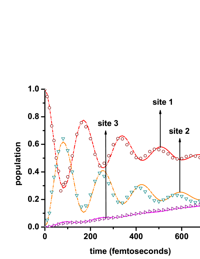
Figure 1: Calculations for the spectral density $J_{D}(\omega)$. Initial excitation is on site 1 and temperature is 77 K. Comparison of our results (dashed lines) with those of Nalbach et al.Nalbach et al. (2011) (denoted by symbols) for chromophores 1,2 and 3.

With our approach, it is possible to look at the effect of decoherence and population relaxation separately. First, we consider the case when the initial excitation is put on site 1 and the environment is absent. The excitation mostly oscillates between sites 1 and 2 and a very small amount of the total excitation is transferred to the other sites, including site 3 which has the least energy. This is due to the strong off-diagonal coupling in the Hamiltonian between chromophores 1 and 2. If we confine the initial excitation to chromophore 6 and again consider the environment to be absent, the excitation oscillates among the sites 6, 5, 4 and 7 but there is again no appreciable transfer to chromophore 3 which is closest to the reaction centre. We now investigate the impact of decoherence at two temperatures, 77 K and 300 K, respectively. Figure 2 has the initial excitation on 1 at 77 K and shows only the decoherence effects induced by the environment. We have coherent oscillations of the excitation mostly between chromophores 1 and 2 with no significant transfer elsewhere. The oscillatory behaviour of the excitation gets somewhat damped, due to decoherence, at timescales of $\backsim 750\ fs$. However, once we include the environment - induced population relaxation effects along with decoherence (Figure 3), the oscillations at sites 1 and 2 get damped rapidly (the oscillations reduce significantly at $\sim 750\ fs$) and their amplitudes decrease significantly. Chromophore 3 now has a significant amount of excitation transferred to it and it exhibits oscillations only upto $300\ fs$. As there was no appreciable transfer to site 3 in the absence of population relaxation, this is just the environment assisted transport, suggested previously by other authors. There is also some population transfer to chromphore 4 which hardly shows any oscillatory behaviour.

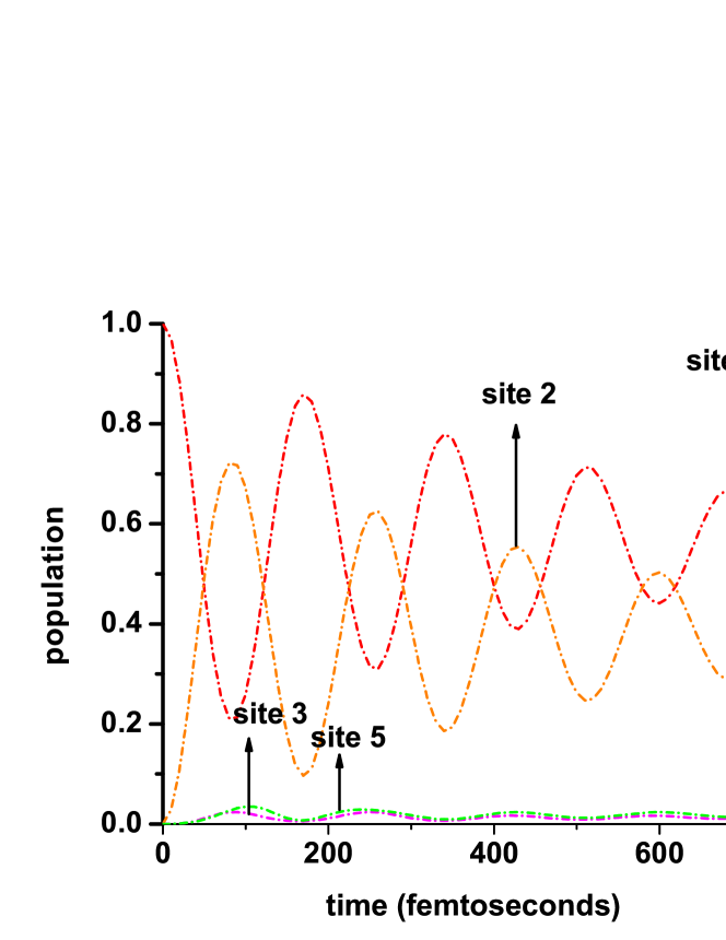
Figure 2: Results for decoherence caused by the environment when the spectral density is $J_{D}(\omega)$ and $T=77K$. Initial excitation is put on site 1. The curves for sites 4, 6 and 7 are not shown as the population at these sites are less than that of site 3 at all times.

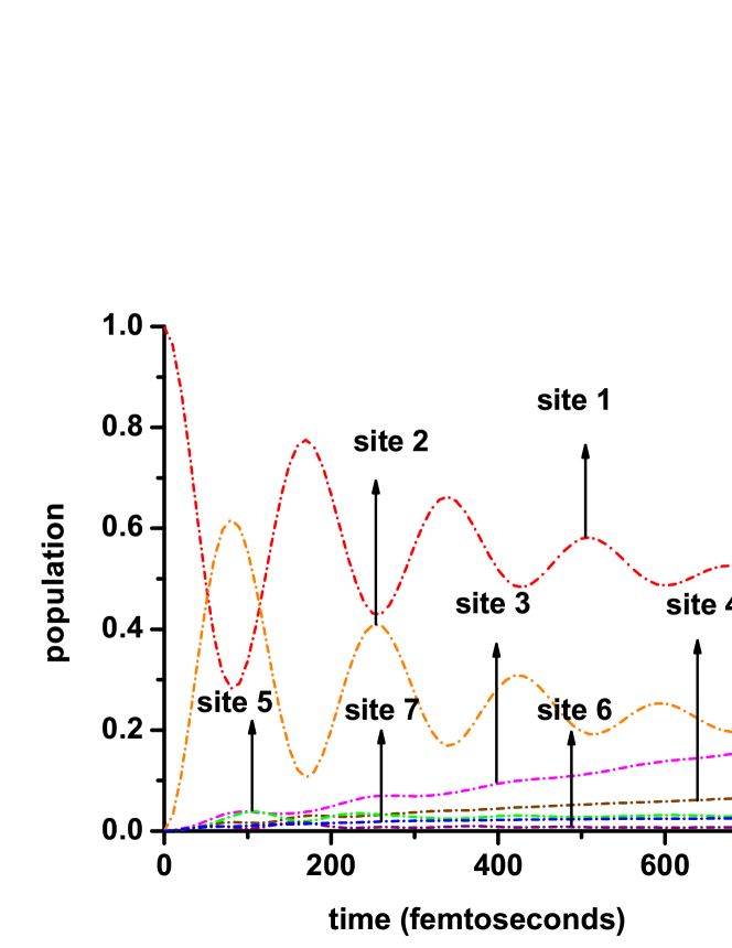
Figure 3: Calculations for spectral density $J_{D}(\omega)$. Initial excitation is taken to be on site 1 and temperature to be 77 K. Curves shown include effects of decoherence and population relaxation due to the environment.

We now consider the environment - induced effects at a higher temperature, 300 K. Figure 4 considers only the decoherence effects on population evolution at the different chromophores with the initial population at site 1. A higher temperature causes severe damping in the oscillatory behaviour of the excitation, which is again mostly confined to sites 1 and 2. The other sites do not receive any appreciable amount of energy. But on inclusion of the population relaxation effects as well (Figure 5), we see the excitation getting transferred to other sites with significant transfers to sites 3 and 4. However the coherent oscillations get damped and disappear around $350\ fs.$

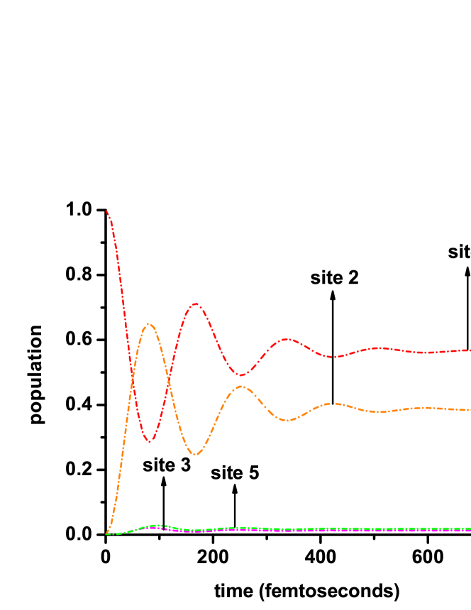
Figure 4: Calculations at 300 K, for the spectral density $J_{D}(\omega)$. Initial excitation is assumed to be on site 1. Calculations account only for decoherence and does not include population relaxation. The curves for sites 4, 6 and 7 are not shown as the population at these sites are less than that of site 3 at all times.

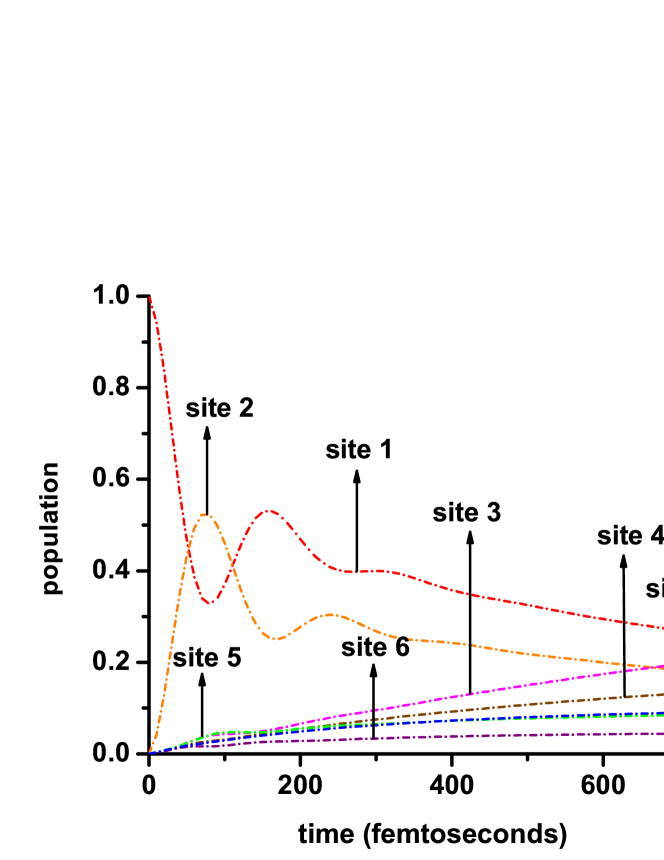
Figure 5: Calculations at 300 K, for spectral density $J_{D}(\omega)$. Initial excitation is assumed to be on site 1. Results include both decoherence and population relaxation due to the environment.

We now consider the initial excitation to be at site 6 and investigate the decoherence effects due to the environment, with and without population relaxation, at the two temperatures. Figures 6 and 7 show only the decoherence effects at 77 K and 300 K respectively. In both the cases, the excitation mostly oscillates between chromophores 6, 5, 4 and 7 with no significant transfer elsewhere, as in the case where the environment was considered absent. However, higher the temperature we consider, greater would be the damping and the coherent oscillations would disappear faster. At 77 K, the oscillations, though damped, persist upto $\backsim 500\ fs$. However, at 300 K, the oscillations disappear around $\backsim 200\ fs$.

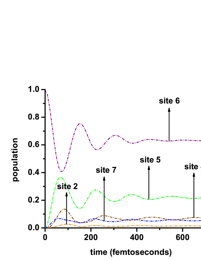
Figure 6: Calculations for the spectral density $J_{D}(\omega)$ and temperature 77 K. Initial excitation is assumed to be on site 6. The curves include only the effects of decoherence and do not include effects of population relaxation. The curves for sites 1 and 3 are not shown as the population at these sites are less than that of site 2 at all times.

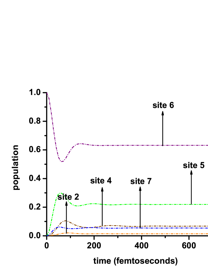
Figure 7: Calculations for the spectral density $J_{D}(\omega)$ and temperature 77 K. Initial excitation is assumed to be on site 6. The curves include only the effects of decoherence and do not include effects of population relaxation. The curves for sites 1 and 3 are not shown as the population at these sites are less than that of site 2 at all times.

Inclusion of the population relaxation effects (Figures 8 and 9) results in faster damping and more importantly, in transfer of the population to the other sites, most importantly to chromophore 3, which is located closest to the reaction centre and chromophore 4. Again, thermal equilibrium is attained faster at higher temperatures.

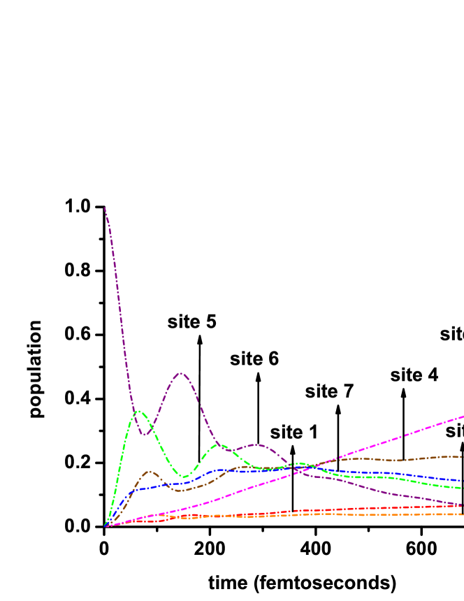
Figure 8: Calculations for the spectral density $J_{D}(\omega)$ and temperature 77 K. Initial excitation is assumed to be on site 6. The curves include effects of both decoherence and population relaxation due to the environment.

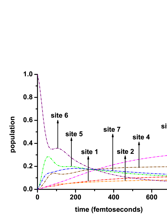
Figure 9: Calculations for the spectral density $J_{D}(\omega)$ and temperature 300 K. Initial excitation is assumed to be on site 6. The curves include effects of both decoherence and population relaxation due to the environment.

We now present the calculations for the more realistic spectral density $J_{AR}(\omega)$ suggested by Adolphs and Rengers Adolphs and Renger (2006), for which exact numerical calculations have been done by Nalbach and coworkers Nalbach et al. (2011). We show only the results which arise from decoherence and population relaxation considered together. Again, we provide a comparison of our results with them to show how well the method works, despite the approximations in Figure 10. The agreement is seen to be very good.

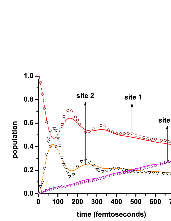
Figure 10: Calculations for the spectral density $J_{AR}(\omega)$. We have taken $\gamma_{p}=1\ cm^{-1}$ and temperature to be 77 K. Initial excitation is taken to be on site 1. The curves include effects of decoherence and population relaxation due to the environment. The figure compares our results (lines) with those of Nalbach et al.Nalbach et al. (2011) (denoted by symbols) for chromophores 1, 2 and 3 and the agreement is found to be good.

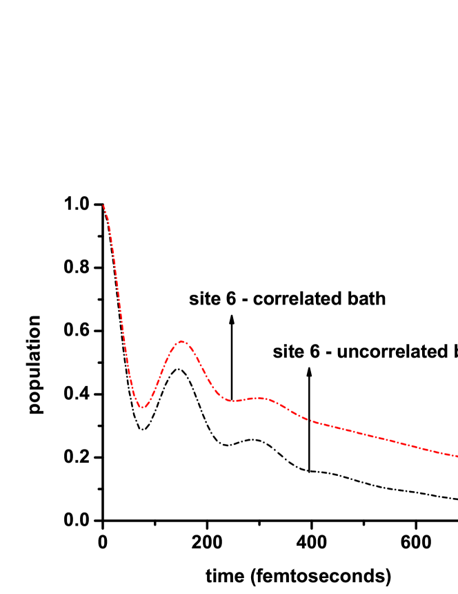
Figure 11: Calculations for the spectral density $J_{D}(\omega)$. Initial excitation assumed to be on site 6 and the temperature is taken to be 77 K. Results are given for the population on site 6, for both correlated and uncorrelated baths.

Figure 12: Calculations for the spectral density $J_{D}(\omega)$. Initial excitation is assumed to be on site 6 at 77 K. The plots show probability of transfer to site 3, for correlated and uncorrelated baths.

VII Correlated Bath

It is also possible to investigate, how the presence of correlations among the bath degrees of freedom affects the process of light-harvesting Sarovar et al. (2011). A numerical investigation of the effect of correlations on the simple two level system was done by Nalbach and coworkers Nalbach et al. (2010). We investigate the effect of correlations for the seven level system using our method. Reference Sarovar et al. (2011) suggests three different models for correlations. The first has no correlations, which is what we have studied in detail in this paper. The second one has correlations between neighboring sites while the third has correlations decay exponentially with distance. We have studied the second model, as we wish to see what happens if correlations are included. Physically, it seems unlikely that there are correlations, as the sites are rather apart in space. It should be pointed out that recent simulations Olbrich et al. (2011) found no correlations in the fluctuations of the energies at different sites. A quantitative measure of the spatial correlation is given by the correlation matrix $C$ of Eq. (9). Following reference Sarovar et al. (2011), we use $C_{12}=C_{21}=C_{56}=C_{65}=0.9;C_{45}=C_{54}=C_{47}=C_{74}=0.4.$ Figures 11 and 12 compare the evolution of population for correlated and uncorrelated bath for two specific cases: a) population evolution at site 6 when the initial excitation is at site 6 at 77 K and b) population evolution at site 3 when the initial excitation is at site 6 at 77 K. The spectral density used here is the Drude spectral density. From Figure 11, we see that in the absence of correlations, the population at site 6 reaches thermal equilibrium faster. However, we would be more interested in the excitation transfer to site 3 as it sits closest to the reaction centre. In Figure 12, the excitation is transferred much faster and hence more efficiently to site 3 in the absence of correlations. It has been recently suggested that vibrational coherences may be responsible for the oscillations that are observed in the experiments with the FMO complex Chin et al. (2013); Tiwari et al. (2013); Polyutov et al. (2012); Christensson et al. (2012). This requires that one or more vibrations exchange energy back and forth with electronic excitations. Proper accounting for this requires that these vibrations should be accounted for in a more detailed manner than we have done. We are currently investigating the extension of our approach to account for this. Also, it has been suggested that the initial state that is produced in the experiment may not be on a single site, but it may be delocalized over two (or more) sites. In our approach this is quite easy to account for - all that one needs is to express the initial state in terms of the delocalized eigenfunctions. We are currently investigating such states using the method.

VIII Conclusions

In this paper, we have introduced an analytical technique for treating coherent wavelike excitation transfer. We wish to emphasize that unlike the existing numerical techniques, the method is computationally inexpensive and could be applied to systems with large number of states. Again, the existing approaches mostly employ perturbative techniques. However, our treatment, which employs mapping onto the adiabatic basis, accounts for decoherence and population relaxation independently. Decoherence is accounted for non-perturbatively, and population relaxation using a Markovian master equation. Results are presented for two spectral densities: a) Drude spectral density and b) the spectral density determined by Adolphs and Renger Adolphs and Renger (2006) for the FMO complex. The results obtained suggest that if only the environment-induced decoherence is considered, there is only damping observed in the oscillatory nature of the excitation which otherwise remains confined to the same sites as in the case where we have considered the environment absent. A higher temperature would only induce more severe damping. In other words, on confining the initial excitation to site 1 or site 6, coherence doesn’t help the excitation propagate to site 3 which has the least energy and is located closest to the reaction centre where the electron transfer reaction takes place. The energy transfer to site 3 and the other sites takes place only when the population relaxation effects are included along with coherence effects. Again, at higher temperatures, attainment of thermal equilibrium due to this would be faster. Therefore, the population relaxation, which is responsible for washing out of the coherences, is the principal reason for the excitation to move to site 3. The coherent oscillations, which do not persist for large enough times, remain essentially confined to a subset of chromophores and do not help in propagating the excitation to site 3. The method also works well when we use the spectral density suggested by Adolphs and Renger Adolphs and Renger (2006), which has a discrete mode too. We also investigate the effects of presence of bath correlations. The excitation transfer to the reaction centre is more efficient in their absence. To conclude, the extremely efficient light harvesting phenomenon is rendered so by the dissipative influence of the environment and not its absence, as usually suspected.

IX Acknowledgements

The work of K.L. Sebastian was supported by the Department of Science and Technology, Govt. of India by the J.C. Bose fellowship program. Pallavi Bhattacharyya thanks the Indian Institute of Science for scholarship.

Appendix A Evaluating the Decoherence Terms

We can evaluate $Tr_{ph}\left\{\left(\hat{T}e^{-i\int_{0}^{t}dt_{1}\varepsilon_{n}(\mathbf{Q}(t_{1}))/\hbar}\right)\rho_{ph}(0)\left(\hat{T}^{\dagger}\,e^{i\int_{0}^{t}dt_{1}\varepsilon_{n^{\prime}}(\mathbf{Q}(t_{1}))/\hbar}\right)\right\}$ in the following manner: We have from Eq. (19)

$$\overline{H}_{0}=\sum_{m}\varepsilon_{m}(\mathbf{Q})c_{m}^{\dagger}c_{m}+\frac{1}{2}\sum_{j,k}\left\{\frac{\widehat{p}_{jk}^{2}}{m_{jk}}+m_{jk}\omega_{jk}^{2}q_{jk}^{2}\right\}$$

We consider upto first order in $\varepsilon_{m}(\mathbf{Q})$ with respect to $Q$. Consequently, $\varepsilon_{m}(\mathbf{Q})=\varepsilon_{m}^{0}+\sum_{j}\left(\frac{\partial\varepsilon_{m}}{\partial Q_{j}}\right)_{Q_{j}=0}Q_{j}$ . Therefore, $\overline{H}_{0}=H_{0}+V\,$ where $H_{0}=\sum_{m}\varepsilon_{m}^{0}c_{m}^{\dagger}c_{m}+\frac{1}{2}\sum_{j,k}\left\{\frac{\widehat{p}_{jk}^{2}}{m_{jk}}+m_{jk}\omega_{jk}^{2}q_{jk}^{2}\right\}$ and $V=\sum_{j,m}\left(\frac{\partial\varepsilon_{m}}{\partial Q_{j}}\right)_{Q_{j}=0}Q_{j}\,c_{m}^{\dagger}c_{m}$. Now we write the following matrix element in the interaction picture as follows:

$$Tr_{ph}\left\{\left(\hat{T}e^{-i\int_{0}^{t}dt_{1}\varepsilon_{n}(\mathbf{Q}(t_{1}))dt_{1}/\hbar}\right)\rho_{ph}(0)\left(\hat{T}^{\dagger}\,e^{i\int_{0}^{t}dt_{1}\varepsilon_{n^{\prime}}(\mathbf{Q}(t_{1}))dt_{1}/\hbar}\right)\right\}$$

$$=Tr_{ph}\left\{\left\langle n\left|e^{-i\overline{H}_{0}t/\hbar}\right|n\right\rangle\rho_{ph}(0)\left\langle n^{\prime}\left|e^{i\overline{H}_{0}t/\hbar}\right|n^{\prime}\right\rangle\right\}$$

$$=Tr_{ph}\left\{\left\langle n\left|e^{-iH_{0}t/\hbar}e^{iH_{0}t/\hbar}e^{-i\overline{H}_{0}t/\hbar}\right|n\right\rangle\rho_{ph}(0)\left\langle n^{\prime}\left|e^{i\overline{H}_{0}t/\hbar}e^{-iH_{0}t/\hbar}e^{iH_{0}t/\hbar}\right|n^{\prime}\right\rangle\right\}$$

$$=e^{-i\varepsilon_{nn^{\prime}}t/\hbar}Tr_{ph}\left\{\left\langle n\left|e^{iH_{0}t/\hbar}e^{-i\overline{H}_{0}t/\hbar}\right|n\right\rangle\rho_{ph}(0)\left\langle n^{\prime}\left|e^{i\overline{H}_{0}t/\hbar}e^{-iH_{0}t/\hbar}\right|n^{\prime}\right\rangle\right\}$$

$$=e^{-i\varepsilon_{nn^{\prime}}t/\hbar}Tr_{ph}\left\{\left(\hat{Te^{-i\int_{0}^{t}dt_{1}V_{I}\left(t_{1}\right)/\hbar}}\,\right)\rho_{ph}(0)\left(\hat{T}^{\dagger}e^{i\int_{0}^{t}dt_{1}V_{I}\left(t_{1}\right)/\hbar}\right)\right\}$$

Using cumulant expansion and writing $Q_{j}(t)$ in terms of creation and annihilation operators, the above expression can be evaluated. Then we get

$$Tr_{ph}\left\{\left(\hat{T}e^{-i\int_{0}^{t}dt_{1}\varepsilon_{n}(\mathbf{Q}(t_{1}))/\hbar}\right)\rho_{ph}(0)\left(\hat{T}^{\dagger}\,e^{i\int_{0}^{t}dt_{1}\varepsilon_{n^{\prime}}(\mathbf{Q}(t_{1}))/\hbar}\right)\right\}=e^{-i\varepsilon_{nn^{\prime}}t/\hbar}e^{-\phi_{n,n^{\prime}}(t)}.$$

where $\varepsilon_{nn^{\prime}}=\varepsilon_{n}^{0}-\varepsilon_{n^{\prime}}^{0}$,

$$Re(\phi_{n,n^{\prime}}(t))=\frac{1}{\hbar}\int_{0}^{\infty}d\omega J(\omega)\frac{1-\cos(\omega t)}{\omega^{2}}\coth\left(\frac{\beta\hbar\omega}{2}\right)\sum_{j=1,2,...,7}\left(\frac{\partial\varepsilon_{n}}{\partial Q_{j}}-\frac{\partial\varepsilon_{n^{\prime}}}{\partial Q_{j}}\right)_{Q_{j}=0}^{2}$$ (52)

and

$$Im(\phi_{n,n^{\prime}}(t))=\frac{1}{\hbar}\int_{0}^{\infty}d\omega J(\omega)\frac{\sin(\omega t)-\omega t}{\omega^{2}}\sum_{j=1,2,...,7}\left(\left(\frac{\partial\varepsilon_{n}}{\partial Q_{j}}\right)_{Q_{j}=0}^{2}-\left(\frac{\partial\varepsilon_{n^{\prime}}}{\partial Q_{j}}\right)_{Q_{j}=0}^{2}\right)$$ (53)

We now evaluate the two integrals. First in Eq. (42), we rewrite

$$\frac{1}{\hbar}\int_{0}^{\infty}d\omega J(\omega)\frac{1-\cos(\omega t)}{\omega^{2}}\coth\left(\frac{\beta\hbar\omega}{2}\right) = \frac{1}{2\hbar}\int_{0}^{t}dt_{2}\int_{0}^{t_{2}}dt_{1}\int_{-\infty}^{\infty}d\omega J(\omega)e^{i\omega t_{1}}\coth\left(\frac{\beta\hbar\omega}{2}\right).$$ (54)

Using Drude spectral density, $\int_{-\infty}^{\infty}d\omega J(\omega)e^{i\omega t_{1}}\coth\left(\frac{\beta\hbar\omega}{2}\right)=\frac{2\lambda}{\pi}\int_{-\infty}^{\infty}d\omega\frac{\omega}{\omega^{2}+\omega_{C}^{2}}e^{i\omega t_{1}}\coth\left(\frac{\beta\hbar\omega}{2}\right)$ which can be evaluated using contour integration. The above function has poles at $\omega=\pm i\pi,\pm i\frac{2\pi n}{\beta\hbar}\,(n=0,1,2,...)$. Applying the Cauchy Integral theorem at the poles and evaluating the time-integration, we have

$$\frac{1}{\hbar}\int_{0}^{\infty}d\omega J(\omega)\frac{1-\cos(\omega t)}{\omega^{2}}\coth\left(\frac{\beta\hbar\omega}{2}\right)$$

$$= \frac{\lambda}{\hbar\omega_{c}}\,\cot\left(\frac{\beta\hbar\omega_{c}}{2}\right)\left(e^{-\omega_{c}t}+\omega_{c}t-1\right)$$ (55)

$$+\frac{4\lambda\omega_{c}}{\hbar^{2}\beta}\sum_{n=1}^{\infty}\frac{1}{\nu_{n}\left(\nu_{n}^{2}-\omega_{c}^{2}\right)}\left(e^{-\nu_{n}t}+\nu_{n}t-1\right).$$

Here, $\nu_{n}=\frac{2\pi n}{\beta\hbar}$. Eq. (43) could easily be evaluated to give the following expressions:

$$\frac{1}{\hbar}\int_{0}^{\infty}d\omega J(\omega)\frac{\sin(\omega t)-\omega t}{\omega^{2}}=-\frac{\lambda}{\hbar\omega_{c}}\left(e^{-\omega_{c}t}+\omega_{c}t-1\right).$$ (56)

Therefore,

$$Re(\phi_{n,n^{\prime}}(t))=\left(\frac{\lambda}{\hbar\omega_{c}}\,\cot\left(\frac{\beta\hbar\omega_{c}}{2}\right)\left(e^{-\omega_{c}t}+\omega_{c}t-1\right)+\frac{4\lambda\omega_{c}}{\hbar^{2}\beta}\sum_{n=1}^{\infty}\frac{1}{\nu_{n}\left(\nu_{n}^{2}-\omega_{c}^{2}\right)}\left(e^{-\nu_{n}t}+\nu_{n}t-1\right)\right)$$

$$\sum_{j=1,2,...,7}\left(\frac{\partial\varepsilon_{n}}{\partial Q_{j}}-\frac{\partial\varepsilon_{n^{\prime}}}{\partial Q_{j}}\right)_{Q_{j}=0}^{2}$$ (57)

and

$$Im(\phi_{n,n^{\prime}}(t))=\left(-\frac{\lambda}{\hbar\omega_{c}}\left(e^{-\omega_{c}t}+\omega_{c}t-1\right)\right)\sum_{j=1,2,...,7}\left(\left(\frac{\partial\varepsilon_{n}}{\partial Q_{j}}\right)_{Q_{j}=0}^{2}-\left(\frac{\partial\varepsilon_{n^{\prime}}}{\partial Q_{j}}\right)_{Q_{j}=0}^{2}\right).$$ (58)

Appendix B Deriving the Master Equation

In this section, we give a brief derivation of the master equation. The approach is well known and is used in several papers Leegwater et al. (1997); Kuehn and Sundstroem (1997); Zhang et al. (1998); Yang and Fleming (2002); Renger and May (1998); Renger and Marcus (2003, 2003). As is usual in deriving master equations DiVentra (2008), we introduce two projection operators $\mathbb{A}$ and $\mathbb{B}$ which are defined by

$$\mathbb{A}X=\rho_{ph}\left(0\right)Tr_{ph}X$$ (59)

$$\mathbb{B}X=\left(1-\mathbb{A}\right)X$$ (60)

for any operator $X$. Using these and following DiVentra (2008), we derive the equations:

$$\frac{\partial\widetilde{\rho}_{1}(t)}{\partial t}=\mathbb{A}L_{na}(t)\widetilde{\rho}_{1}(t)+\mathbb{A}L_{na}(t)\widetilde{\rho}_{2}(t),$$ (61)

and

$$\frac{\partial\widetilde{\rho}_{2}(t)}{\partial t}=\mathbb{B}L_{na}(t)\widetilde{\rho}_{1}(t)+\mathbb{B}L_{na}(t)\widetilde{\rho}_{2}(t),$$ (62)

where $\widetilde{\rho}_{1}(t)=\mathbb{A}\widetilde{\rho}_{nn^{\prime}}(t)$ and $\widetilde{\rho}_{2}(t)=\mathbb{B}\widetilde{\rho}_{nn^{\prime}}(t)$. Note that $\rho_{1}(t)$ and $\rho_{2}(t)$, are dependent on the initial coherence $|n\rangle\langle n^{\prime}|$, which we have not indicated explicitly as that will clutter up the notation. It is easy to show that $\mathbb{A}L_{na}(t)\widetilde{\rho}_{1}(t)=0$. Solving Eq. (62) and using it in Eq. (61) we get

$$\frac{\partial\widetilde{\rho}_{1}(t)}{\partial t}=Tr_{ph}\left\{L\left(t\right)\int_{0}^{t}dt_{1}e^{\mathbb{B}L_{na}\left(t-t_{1}\right)}L_{na}\left(t_{1}\right)\widetilde{\rho}_{ph}\left(0\right)\right\}\widetilde{\rho}_{1}(t_{1}).$$ (63)

As this is expected to be small, in Eq. (63) we retain terms upto second order in $L_{na}(t)$. This implies that we shall approximate $e^{BL_{na}\left(t-t_{1}\right)}\approx 1$. Further, we make the Markovian approximation and put $\widetilde{\rho}_{1}(t_{1})\approx\widetilde{\rho}_{1}(t)$ and take the upper limit in the integral to be infinity, to get

$$\frac{\partial\widetilde{\rho}_{1}(t)}{\partial t}=Tr_{ph}\left\{\int_{0}^{\infty}dt_{1}L_{na}\left(t\right)L_{na}\left(t_{1}\right)\widetilde{\rho}_{ph}\left(0\right)\right\}\widetilde{\rho}_{1}(t).$$ (64)

On evaluating the right hand side of the above expression, we get

$$\frac{\partial\widetilde{\rho}_{1}(t)}{\partial t}=-\sum_{r,r^{\prime},s}B_{r,r^{\prime},s}[X_{r^{\prime},s}|r\rangle\langle s|\widetilde{\rho}_{1}(t)+X_{r^{\prime},r}\widetilde{\rho}_{1}(t)|r\rangle\langle s|]+\sum_{r,r^{\prime},s^{\prime},s}B^{\prime}_{r,r^{\prime},s^{\prime},s}(X_{r,r^{\prime}}+X_{s^{\prime},s})[|r\rangle\langle r^{\prime}|\widetilde{\rho}_{1}(t)|s^{\prime}\rangle\langle s|],$$ (65)

with the initial condition $\widetilde{\rho}_{1}(0)=|n\rangle\langle n^{\prime}|$. $|r\rangle$, $|r^{\prime}\rangle$, $|s^{\prime}\rangle$ and $|s\rangle$ are the adiabatic states evaluated at $\mathbf{Q=0}.$ $B_{r,r^{\prime},s}=\sum_{j}A_{r,r^{\prime},\mathbf{0}}^{j}A_{r^{\prime},s,\mathbf{0}}^{j}$; $B^{\prime}_{r,r^{\prime},s^{\prime},s}=\sum_{j}A_{r,r^{\prime},\mathbf{0}}^{j}A_{s^{\prime},s,\mathbf{0}}^{j}$ and $\omega_{rr^{\prime}}=(\varepsilon_{r}^{0}-\varepsilon_{r^{\prime}}^{0})/\hbar$.

$$X_{r,r^{\prime}}=\begin{cases}\frac{\pi}{\hbar}\frac{J(\omega_{rr^{\prime}})\omega_{rr^{\prime}}^{2}}{e^{\beta\hbar\omega_{rr^{\prime}}}-1}&\mbox{if }\omega_{rr^{\prime}}>0\\ \frac{\pi}{\hbar}\frac{J(\omega_{r^{\prime}r})\omega_{r^{\prime}r}^{2}}{1-e^{-\beta\hbar\omega_{r^{\prime}r}}}&\mbox{if }\omega_{r^{\prime}r}>0.\end{cases}$$ (66)

Here $J_{j}(\omega)$ is the spectral density defined as

$$J_{j}(\omega)=\sum_{k}\frac{m_{jk}\nu_{jk}^{2}}{2\omega_{jk}}\delta(\omega-\omega_{jk}).$$ (67)

References

- Brixner et al. (2005) T. Brixner, J. Stenger, H. Vaswani, M. Cho, R. Blankenship, and G. Fleming, Nature, 434, 625 (2005).
- Engel et al. (2007) G. Engel, T. Calhoun, E. Read, T.-K. Ahn, T. Mancal, Y.-C. Cheng, R. Blankenship, and G. Fleming, Nature, 446, 782 (2007).
- Read et al. (2007) E. Read, G. Engel, T. Calhoun, T. Mancal, T. Ahn, R. Blankenship, and G. Fleming, Proceedings of the National Academy of Sciences of the United States of America, 104, 14203 (2007).
- Leegwater et al. (1997) J. A. Leegwater, J. R. Durrant, and D. R. Klug, The Journal of Physical Chemistry B, 101, 7205 (1997), http://pubs.acs.org/doi/pdf/10.1021/jp9634058 .
- Kuehn and Sundstroem (1997) O. Kuehn and V. Sundstroem, Journal of Chemical Physics, 107, 4154 (1997).
- Renger and May (1998) T. Renger and V. May, The Journal of Physical Chemistry A, 102, 4381 (1998), http://pubs.acs.org/doi/pdf/10.1021/jp9800665 .
- Fenna and Matthews (1975) R. Fenna and B. Matthews, Nature, 258, 573 (1975).
- Li et al. (1997) Y.-F. Li, W. Zhou, R. Blankenship, and J. Allen, The Journal of Molecular Biology, 271, 456 (1997).
- Camara-Artigas et al. (2003) A. Camara-Artigas, R. Blankenship, and J. Allen, Photosynthesis Research, 75, 49 (2003).
- Panitchayangkoon et al. (2010) G. Panitchayangkoon, D. Hayes, K. Fransted, J. Caram, E. Harel, J. Wen, R. Blankenship, and G. Engel, Proceedings of the National Academy of Sciences of the United States of America, 107, 12766 (2010).
- Prezhdo and Rossky (1998) O. Prezhdo and P. J. Rossky, Physical Review Letters, 81, 5294 (1998).
- Gilmore and McKenzie (2006) J. Gilmore and R. McKenzie, Chemical physics letters (2006), doi:10.1016/j.cplett.2005.12.104.
- Gilmore and McKenzie (2008) J. Gilmore and R. H. McKenzie, Journal of Physical Chemistry A, 112, 2162 (2008).
- Nalbach et al. (2011) P. Nalbach, A. Ishizaki, G. R. Fleming, and M. Thorwart, New Journal of Physics, 13 (2011a), doi:10.1088/1367-2630/13/6/063040.
- Rebentrost et al. (2009) P. Rebentrost, M. Mohseni, and A. Aspuru-Guzik, The Journal of Physical Chemistry. B, 113, 9942 (2009a).
- Rebentrost et al. (2009) P. Rebentrost, M. Mohseni, I. Kassal, S. Lloyd, and A. Aspuru-Guzik, New Journal of Physics, 11, 033003 (2009b).
- Abramavicius and Mukamel (2010) D. Abramavicius and S. Mukamel, The Journal of chemical physics, 133 (2010), doi:10.1063/1.3493580.
- Singh (2012) N. Singh, arXiv:1203.0147v1 [cond-mat.stat-mech] (2012).
- Ball (2011) P. Ball, Nature, 474, 272 (2011).
- Lloyd (2011) S. Lloyd, Journal of Physics: Conference Series, 302 (2011), doi:10.1088/1742-6596/302/1/012037.
- Ishizaki and Fleming (2009) A. Ishizaki and G. Fleming, Proceedings of the National Academy of Sciences of the United States of America, 106, 17255 (2009a).
- Ishizaki and Fleming (2009) A. Ishizaki and G. Fleming, The Journal of Chemical Physics, 130, 23411 (2009b).
- Mohseni et al. (2008) M. Mohseni, P. Rebentrost, S. Lloyd, and A. Aspuru-Guzik, The Journal of Chemical Physics, 129 (2008), doi:10.1063/1.3002335.
- Caruso et al. (2009) F. Caruso, A. W. Chin, A. Datta, S. F. Huelga, and M. B. Plenio, The Journal of Chemical Physics, 131 (2009), doi:10.1063/1.3223548.
- Olaya-Castro and Scholes (2011) A. Olaya-Castro and G. Scholes, International Reviews in Physical Chemistry, 30, 49 (2011).
- Nalbach et al. (2011) P. Nalbach, D. Braun, and M. Thorwart, Physical Review E, 84, 041926 (2011b).
- Olbrich et al. (2011) C. Olbrich, J. Strümpfer, K. Schulten, and U. Kleinekathofer, The Journal of Physical Chemistry Letters, 2011, 1771 (2011a).
- Mhlbacher and Kleinekathofer (2012) L. Mhlbacher and U. Kleinekathofer, The Journal of Physical Chemistry B, 116, 3900 (2012).
- Weiss (2008) U. Weiss, Quantum Dissipative Systems, 3rd ed., Series in Modern Condensed Matter Physics (World Scientific, Singapore, 2008).
- Orth et al. (2010) P. P. Orth, A. Imambekov, and K. L. Hur, Phys. Rev. A, 82, 032118 (2010a).
- Orth et al. (2010) P. P. Orth, D. Roosen, W. Hofstetter, and K. L. Hur, Phys. Rev. B, 82, 144423 (2010b).
- Schlosshauer (2007) M. Schlosshauer, Decoherence and the Quantum to Classical Transition (Springer, Berlin, 2007).
- Sarovar et al. (2011) M. Sarovar, Y. Cheng, and K. Whaley, Physical Review E, 83, 011906 (2011).
- Ishizaki and Fleming (2009) A. Ishizaki and G. Fleming, The Journal of Chemical Physics, 130, 23411 (2009c).
- Baer (2006) M. Baer, Beyond Born-Oppenheimer. Conical Intersections and Electronic Nonadiabatic Coupling Terms (Wiley-Interscinece, New York, 2006).
- Zhang et al. (1998) W. M. Zhang, T. Meier, V. Chernyak, and S. Mukamel, The Journal of Chemical Physics, 108 (1998), doi:10.1063/1.476212.
- Yang and Fleming (2002) M. Yang and G. Fleming, Chemical Physics, 282, 163 (2002).
- Renger and Marcus (2003) T. Renger and R. A. Marcus, The Journal of Physical Chemistry A, 107, 8404 (2003a), http://pubs.acs.org/doi/pdf/10.1021/jp026789c .
- Renger and Marcus (2003) T. Renger and R. A. Marcus, Journal of Chemical Physics, 116, 9997 (2003b).
- Adolphs and Renger (2006) J. Adolphs and T. Renger, Biophysical Journal, 91, 2778 (2006).
- Nalbach et al. (2010) P. Nalbach, J. Eckel, and M. Thorwart, New Journal of Physics, 12, 065043 (2010).
- Olbrich et al. (2011) C. Olbrich, J. Strümpfer, K. Schulten, and U. Kleinekathofer, The Journal of Physical Chemistry B, 115, 758 (2011b).
- Chin et al. (2013) A. Chin, J. Prior, R. Rosenbach, F. Caycedo-Soler, S. Huelga, and M. Plenio, Nature Physics, 9, 113 (2013).
- Tiwari et al. (2013) V. Tiwari, W. K. Peters, and D. M. Jonas, Proceedings of the National Academy of Sciences, 110, 1203 (2013).
- Polyutov et al. (2012) S. Polyutov, O. Kühn, and T. Pullerits, Chemical Physics, 394, 21 (2012).
- Christensson et al. (2012) N. Christensson, H. Kauffmann, T. Pullerits, and M. T., The Journal of Physical Chemistry B, 116, 7449 (2012).
- DiVentra (2008) M. DiVentra, Electrical Transport in Nanoscale Systems (Cambridge University Press, New Delhi, 2008).