Autonomous search for a diffusive source in an unknown environment

Abstract

The paper presents an approach to olfactory search for a diffusive emitting source of tracer (e.g. aerosol, gas) in an environment with unknown map of randomly placed and shaped obstacles. The measurements of tracer concentration are sporadic, noisy and without directional information. The search domain is discretised and modelled by a finite two-dimensional lattice. The links is the lattice represent the traversable paths for emitted particles and for the searcher. A missing link in the lattice indicates a blocked paths, due to the walls or obstacles. The searcher must simultaneously estimate the source parameters, the map of the search domain and its own location within the map. The solution is formulated in the sequential Bayesian framework and implemented as a Rao-Blackwellised particle filter with information-driven motion control. The numerical results demonstrate the concept and its performance.

I Introduction

The search for an emitting source of particles, chemicals, odour, or radiation, based on sporadic clues or intermittent measurements, has attracted a great deal of interest lately. The topic is important for search and rescue operations with the goal to localise dangerous pollutants, such as chemical leaks and radioactive sources. In biology, the search is studied to model animal bahaviour in search for food or mates [1, 2, 3]. Bio-inspired search for underwater sources of pollution have been studied in [4, 5, 6]. A robot for gas/odour plume tracking guided by the increase in the concentration gradient has been proposed in [7]. “Infotaxis” [8] is a search strategy based on entropy-reduction maximisation which has been developed in the context of finding a weak source in a turbulent flow (e.g. drug or leak emitting chemicals, for a comprehensive review see [9]). Information-gain driven search for radioactive point sources has been studied in [10]. In all these applications the search domain is either open (without obstacles) or a precise map of the search domain (with obstacles) is available.

In this paper we focus on autonomous olfactory search for a diffusive emitting source of tracer (e.g. aerosol, gas, heat, moisture) in a domain with randomly placed and shaped obstacles (forbidden areas), whose structure (the map) is unknown. The problem is of importance for example in localisation of dangerous leaks in collapsed buildings, inside tunnels or mines. The searcher senses in a probabilistic manner both the structure of the search domain (e.g. the presence or absence of obstacles, walls, blocked passages) and the level of concentration of tracer particles. The objective of the search is to localise and report the coordinates of the source in a shortest possible time. This is not a trivial task for several reasons. First, the emission rate of the source is typically unknown. Furthermore, the measurements of tracer particle concentration are sporadic, noisy and without directional information. Since the structure (map) of the search domain is unknown, the searcher needs to explore the domain and create its map. The searcher motion is fully autonomous: it senses the environment and after processing this uncertain information sequentially makes decisions on where to move next in order to collect new measurements. Its motion control, however, is not fully reliable as it may occasionally fail to execute correctly. The probabilistic model of searcher motion is assumed known.

In the paper we restrict to the search in a two-dimensional domain. The coordinates of the searcher initial position, as well as the border of the search area (relative to the initial position) are given as input parameters. In order to fulfil its mission, the searcher has to find the source and report its coordinates relative to its initial position. This in turn requires simultaneous estimation at three levels: (1) estimation of source parameters (its location in 2D and its release rate); (2) estimation of the map of the search area and (3) estimation of the searcher position within the estimated map. Estimation at levels (2) and (3) has been studied extensively in robotics under the term grid-based simultaneous localisation and mapping (SLAM) [11]. The primary mission in all SLAM publications is an accurate mapping of the area. The primary mission of our searcher, however, is to localise the source, while SLAM is only a necessary component of the solution.

The only related work which deals with olfactory search in an unknown structured environment is [12]. While this paper presents a plethora of experimental results, the algorithms are based on heuristics. Our approach, however, is theoretically sound in the sense that its mathematical models are precisely defined, estimation is carried out in the sequential Bayesian framework and the searcher motion control is driven by information gain.

The search domain is discretised, as for example in [4], and modelled by a finite two-dimensional lattice. With sufficiently fine resolution of the lattice, the emitting source can be considered to be in one of the nodes of the lattice. The links (bonds, edges) of the lattice represent the traversable paths for emitted particles (tracer) and for the searcher. Missing links in the lattice indicate blocked paths due to the walls or obstacles. This is a very general model applicable to searches at various scales, from inside buildings and tunnels, to within cells of living organisms [2]. The percentage of missing links in the lattice is assumed to be above the percolation threshold $p_{c}$ (for the adopted lattice structure $p_{c}=1/2$ [13, 14]) so that long-range connectivity is satisfied [13]. Using the absorbing Markov chains technique [15], we can compute exactly the mean concentration level in any node of the lattice, that is at any point of the search domain with obstacles.

Since the structure (map) of the search domain is unknown, the searcher must rely on a theoretical model of concentration measurement which is independent of the this map. Such a model is derived in the paper in the analytic form and used in the search.

The search itself consist of algorithms for sequential estimation and motion control. We adopt the framework of optimal sequential Bayesian estimation with information-driven motion control. Implementation is carried out using a Rao-Blackwellised particle filter.

The paper is organised as follows. Mathematical models of measurements and searcher motion are described in Sec.II. The olfactory search problem is formulated and its conceptual solution provided in Sec.III. Full technical details of the proposed search algorithm are presented in Sec.IV, with numerical results given in Sec.V. Finally, conclusions of this study are summarised in Sec. VI.

II Modelling

II-A Model of environment

The concentration of a tracer at any point of the search domain is governed by the diffusive equation, which in the steady state reduces to the Laplace equation [16]:

$$D_{0}\;\Delta\theta=A_{0}\,\delta(x-X_{,}y-Y).$$ (1)

Here $D_{0}$ is the diffusion coefficient of tracer in the environment, $\Delta$ is the Laplace operator, $\theta$ is the mean (time-averaged) tracer concentration, $\delta$ is the Dirac delta function, $A_{0}$ is the release-rate of the tracer source, and $X,Y$ are the coordinates of the source in a two-dimensional Cartesian coordinate system. For convenience we adopt a circular search domain of radius $R_{0}$, centred at the origin of the coordinate system, that is for every point inside the search area, $r=\sqrt{x^{2}+y^{2}}\leq R_{0}$. Assuming that the tracer source is undetectable outside the search domain, we can impose the absorbing boundary condition $\theta(r=R_{0})=0$. The traditional approach to the computation of the tracer concentration $\theta$ at every point of the search domain, is via analytical or numerical solution of (1). This, however, is a non-trivial task when the search domain is a structure of complex topology (due to obstacles, compartments walls, random openings, etc).

We therefore adopt an alternative approach, where the continuous model of the tracer diffusion process is replaced with a random walk on a square lattice, adopted as a discrete model of the search area. Discretisation is illustrated in Fig.1 for a search area centred at the origin of the coordinate system, with the radius $R_{0}=9$. The length of each link (edge, bond) in the lattice determines the resolution of discretisation, and in this example is adopted as a unit length. The source, assumed to be located at one of the nodes of the lattice, is emitting particles which travel through the lattice according to the random walk model [17].

     

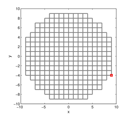
Figure 1: Search area discretisation: the complete grid, with the length of each link equal $1$. The centre of the search area is in $(0,0)$, its radius is $R_{0}=9$.

The obstacles in the search domain (the regions through which the tracer cannot pass) are simply modelled as missing links (or clusters of missing links) in the square lattice. Fig.2 shows an example of such a model: this incomplete lattice is obtained by removing fraction $p=0.35$ of the links in the complete lattice shown in Fig.1. Note that all nodes in the incomplete lattice (grid) are connected. On average this will be the case if the fraction of missing links in the incomplete grid of Fig.2 is below the percolation threshold $p_{c}$; above the percolation threshold ($p>p_{c}$) the lattice becomes fragmented. The framework of percolation theory enables analytical description of statistical properties of such a lattice [13], [14].

     

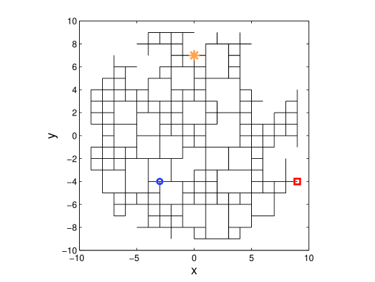
Figure 2: A model of search area with obstacles: the missing links of the complete graph of Fig.1 represent blocked passages (due to the walls, closed doors, etc) for moving particles. This incomplete grid is obtained by removing fraction $p=0.35$ of the links from the complete graph.

II-B Model of tracer distribution

This section explains how to compute the mean concentration of tracer particles in each node of the incomplete grid (such as the one shown in Fig.2) which represents a discretised model of the search area with obstacles.

For a given incomplete grid, the mean concentration can be computed using the absorbing Markov chain technique [15]. Neglecting the spatial approximation of the search domain (due to discretisation) and under the assumption that the distribution of particles has reached the steady state, the absorbing Markov chain technique provides an exact solution for the quantity of source material at each location.

We can regard the random walk of tracer particles through the incomplete grid (e.g. Fig.2) as a Markov chain whose states are the nodes of the grid. The Markov chain is specified by the transition matrix $\mathbf{T}$; each element of this matrix is the probability of transition from state $s_{i}$ to state $s_{j}$ (i.e. a particle move from node $i$ to node $j$): $T_{ij}=P\{s_{j}|s_{i}\}$. How to construct $\mathbf{T}$ given the incomplete grid? First note that we distinguish two types of states in this Markov chain: absorbing states (corresponding to the nodes on the boundary of the grid) and transient states. For an absorbing state $s_{i}$, $\mathbf{T}_{ii}=1$ and $\mathbf{T}_{ij}=0$, if $j\neq i$. Suppose a transient state $s_{i}$ corresponds to node $i$ in the incomplete grid, which has connections (links) with nodes $j_{1},\dots,j_{m}$, where for a square grid $m\leq 4$. Then $\mathbf{T}_{i{j_{1}}}=\dots=\mathbf{T}_{i{j_{m}}}=1/m$ and $\mathbf{T}_{i{j}}=0$ for $j\notin\{j_{1},\dots,j_{m}\}$.

Suppose there are $r$ absorbing states and $t$ transient states. If we order the states so that the absorbing states come first (before the transient states), then the transition matrix takes the canonical form:

$$\mathbf{T}=\left[{\begin{array}[]{cc}~~~~~~~\mathbf{I}&\mathbf{0}\\ ~~~~~~~\mathbf{R}&\mathbf{Q}\\ \end{array}}\right],$$ (2)

where $\mathbf{I}$ is $r\times r$ identity matrix, $\mathbf{Q}$ is the $t\times t$ matrix that describes transitions between transient states, $\mathbf{R}$ is a $t\times r$ matrix that describes the transitions from transient to absorbing states and $\mathbf{0}$ is an $r\times t$ matrix of zeros. The fundamental matrix of the absorbing Markov chain [15],

$$\mathbf{F}=(\mathbf{I}-\mathbf{Q})^{-1},$$ (3)

represents the expected number of visits to a transient state $s_{j}$ starting from a transient state $s_{i}$ (before being absorbed). This matrix will be used in simulations to compute the mean particle concentration in any node of the incomplete grid. Suppose an emitting source is placed at node $i$, which is not on the boundary. The source is releasing tracer particles at a constant rate $A_{0}$. Then the expected concentration of tracer particles in any other node $j$ of the incomplete grid (which is not on the boundary) is given by $\theta_{j}=A_{0}\cdot\mathbf{F}_{ij}$. The concentration scales linearly with the release rate $A_{0}$ as a direct consequence of the linearity of Laplace equation (1).

Fig.3 shows the mean concentration of tracer particles for the search area modelled by incomplete grid of Fig.2, with the source placed at $(X,Y)=(0,7)$ and with $A_{0}=12$. Notice how the concentration depends on the distance from the source and the structure of the grid, plotted in Fig.2.

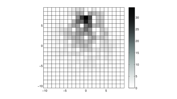
Figure 3: Mean concentration of tracer particles for the search area modelled by incomplete graph of Fig.2 with source placed at $(X,Y)=(0,7)$ with $A_{0}=12$ (darker cells indicate higher concentration)

II-C Sensor models and motion model

Two types of measurements are collected by the searcher. Sensor 1 measures the concentration of tracer particles as a count of particles received during the sampling time. Assuming the so-called ’dilution’ limit (limit of low concentrations) the tracer fluctuations follow the Poisson distribution [8], that is a concentration measurement at node $j$ of the grid is a random sample drawn from

$$n\sim\mathcal{P}(n;\lambda)=\frac{\lambda^{n}}{n!}e^{-\lambda}$$ (4)

where $\lambda=\theta_{j}=A_{0}\cdot\mathbf{F}_{ij}$. The Poisson distribution mimics the intermittency of concentration measurements [8].

The searcher sequentially estimates the source parameters without knowing the map of the search area. Hence the measurement model based on the mean concentration $\lambda=A_{0}\cdot\mathbf{F}_{ij}$ cannot be used in estimation (recall that matrix $\mathbf{F}$ is formed based on the structure of the incomplete grid). Assuming that the fraction of missing links in the incomplete grid is smaller than the percolation threshold $p_{c}$, the expected concentration of tracer particles in any node $j$ of the incomplete grid can be computed approximately using the property of conformal invariance of the Laplace equation (see Appendix for details). Suppose the source of release rate $A_{0}$ is placed at a node of the grid, positioned at coordinates $(X,Y)$. Then the mean (time and ensemble averaged) concentration at node $j$, positioned at $(x_{j},y_{j})$ can be approximated as:

$$\langle\theta\rangle_{j}\approx-\frac{A}{2}\log(R^{2})$$ (5)

where $A=A_{0}/f_{c}$, ($f_{c}$ is a constant, $0<f_{c}<1$, which depends on the fraction of missing links in the incomplete grid, see Appendix), and

$$R^{2}=R^{2}_{0}\frac{(x_{j}-X)^{2}+(y_{j}-Y)^{2}}{(x_{j}Y-y_{j}X)^{2}+(R^{2}_{0}-x_{j}X-y_{j}Y)^{2}}.$$ (6)

Note that this model is independent of the structure of the incomplete grid. In summary, estimation will be carried out using Sensor 1 measurement model based on (4), where mean $\lambda=\langle\theta\rangle_{j}$ is approximated by (5), (6). The actual concentration measurements will be simulated according to (4), but with $\lambda=\theta_{j}=A_{0}\cdot\mathbf{F}_{ij}$.

The searcher moves and explores the search domain in order to find the source. The source parameter estimation is carried out using the map-independent measurement model (5), which does not require discretisation of the search domain on a square lattice (as in Fig.1). Nevertheless, we keep discretisation for the searcher in order to model its motion paths and to facilitate its grid-based SLAM functionality. Thus we assume that the searcher travels within the search area along the paths represented by the links of the incomplete grid as in Fig.2. As it travels, it stops at the nodes along its path to sense the environment, i.e. to collect measurements. Sensor 2 is a simple binary detector of the presence or absence of the links (paths) visible from the node in which the searcher is currently placed. It reports on the presence/absence of the primary and secondary neighbouring links.

A link in a grid of Fig.2, is defined by a quadruple $(x_{1},y_{1},x_{2},y_{2})$, where $(x_{1},y_{2})$ and $(x_{2},y_{2})$ are the coordinates of the nodes it connects. In order to explain what we mean by primary and secondary links, consider for example the node at location $(-3,-4)$ indicated by ’o’ in Fig.2. The primary observable links from this node are the connecting links towards East, West, up and down from $(-3,-4)$, i.e. $\ell_{1}=(-3,-4,-2,-4)$, $\ell_{2}=(-3,-4,-4,-4)$, $\ell_{3}=(-3,-4,-3,-3)$, and $\ell_{4}=(-3,-4,-3,-5)$, i.e. . The status of link $\ell$, $m(\ell)$, takes values from $\{0,1\}$, where $m(\ell)=1$ means that link $\ell$ exists and $m(\ell)=0$ is the opposite. According to Fig.2, $m(\ell_{1})=1$, $m(\ell_{2})=1$, $m(\ell_{3})=0$, $m(\ell_{4})=1$. The secondary observable links from the node at $(-3,-4)$ in Fig.2 represent second neighbouring links in direction of East, West, up and down from $(-1,-1)$, that is $\ell_{5}=(-2,-4,-1,-4)$, $\ell_{6}=(-4,-4,-5,-4)$, $\ell_{7}=(-3,-3,-3,-2)$, and $\ell_{8}=(-3,-5,-3,-6)$. According to Fig.2, $m(\ell_{5})=1$, $m(\ell_{6})=0$, $m(\ell_{7})=0$, $m(\ell_{8})=1$.

Let an observation (supplied by sensor 2) about the presence or absence of a link $\ell$, be a binary value $z(\ell)\in\{0,1\}$, where $z(\ell)=0$ means link $\ell$ is absent and $z(\ell)=1$ is the opposite. The performance od sensor 2 can be described by two detection matrices, one for the primary links, the other for secondary links. Each detection matrix $\Pi$ has a form

$$\Pi=\left[\begin{matrix}P(z=0|m=0)&P(z=0|m=1)\\ P(z=1|m=0)&P(z=1|m=1)\end{matrix}\right].$$ (7)

where $P(z=1|m=1)=p_{d}$ and $P(z=1|m=0)=p_{fa}$ are the probability of correct detection and the probability of false detection $p_{fa}$, respectively. The columns of matrix $\Pi$ add up to $1$, and hence (7) can be written as:

$$\Pi=\left[\begin{matrix}1-p_{fa}&1-p_{d}\\ p_{fa}&p_{d}\end{matrix}\right].$$ (8)

Suppose the searcher is in node $i$ at discrete-time $k-1$. Let the set of admissible controls vectors for the next move be defined as $\mathcal{U}_{k}=\{\cdot,\uparrow,\rightarrow,\downarrow,\leftarrow\}$, meaning that the searcher can stay where it is, or move one unit length up, right, down or left. After processing measurements from its sensors, the searcher decides to choose control $\mathbf{u}^{*}_{k}\in\mathcal{U}_{k}$ and hence to be at time $k$ at node $j$. This control, however, is executed correctly only with probability $1-p_{e}$. Due to control noise or unmodeled exogenous effects [11], with probability $p_{e}$ the searcher will actually execute control $u^{\prime}_{k}\in\mathcal{U}_{k}\setminus\{\mathbf{u}^{*}_{k}\}$.

III The Problem and its Conceptual Solution

The searcher has at its disposal the probabilistic models of sensor measurements and dynamic models. Prior knowledge also includes: (1) the coordinates of its initial position; (2) the length of each link in the square lattice; (3) the boundary of the circular search area (defined by its centre and radius). The described prior translates into knowledge of the complete grid such as the one shown in Fig.1. The searcher cannot move outside the complete grid.

The objective of the searcher is to estimate in the shortest possible time the coordinates of the emitting source, as well as the partial map describing the path from its starting (entry) point to the estimated location of the source. This partial map is important, for example, in order to guide the rescue team to the source or if the searcher has to retreat to its starting position.

III-A Sequential Bayesian estimation

The described problem can be cast in the sequential Bayesian estimation framework as a nonlinear filtering problem. Let us first define the state vector, which consists of three parts:

1. The coordinates of the searcher position at discrete-time $k=1,2,\dots$ are denoted by $\mathbf{p}_{k}=[x_{k}\;\;y_{k}]^{\intercal}$.

2. The status (presence/absence) of each link in the complete grid (such as the one shown in Fig.1). The status of link $\ell_{j}$, where $j=1,\dots,L$, and $L$ is the total number of links in the complete grid, is $m(\ell_{j})=m_{j}\in\{0,1\}$. The notation $P(m_{j}=1)$ refers to the probability that the link is present. The map at time $k$ is fully specified by vector $\mathbf{m}_{k}=[m_{1,k},\dots,m_{L,k}]^{\intercal}$. The time index is introduced because we allow the map of the search area to occasionally change, e.g. an open door can close. The assumption is that the statuses of links are mutually independent, i.e. $m_{j,k}$ is independent from $m_{i,k}$ for $i\neq j$.

3. The parameter vector of the source is denoted by $\mathbf{s}=[X\;\;Y\;\;A]^{\intercal}$.

The complete state vector is then defined as

$$\mathbf{y}_{k}=[\mathbf{p}_{k}^{\intercal}\;\;\mathbf{m}_{k}^{\intercal}\;\;\mathbf{s}^{\intercal}]^{\intercal}.$$

Dynamics of the state $\mathbf{y}_{k}$ is described by two transitional densities: $p(\mathbf{m}_{k}|\mathbf{m}_{k-1})$ specifies the evolution of the map over time, while $p(\mathbf{p}_{k}|\mathbf{p}_{k-1},\mathbf{u}_{k})$ characterises the searcher motion model. The observation models of the searcher are specified by two likelihood functions: $g_{1}(n_{k}|\mathbf{p}_{k},\mathbf{m}_{k},\mathbf{s})$ characterises sensor 1, which provides the count of particles $n_{k}$ at $\mathbf{p}_{k}$ from the source in state $\mathbf{s}$ through the map $\mathbf{m}_{k}$; $g_{2}(\mathbf{z}_{k}|\mathbf{p}_{k},\mathbf{m}_{k})$ refers to sensor 2 and describes the observation $\mathbf{z}_{k}$ of the status of the links in $\mathbf{m}_{k}$ visible from the searcher in location $\mathbf{p}_{k}$. Let us denote observations and controls at time $k$ by a vector $\mbox{\boldmath$\zeta$}_{k}=[n_{k}\;\mathbf{z}_{k}^{\intercal}]^{\intercal}$. Finally, the prior probability density function (PDF) of the state is denoted by $p(\mathbf{y}_{0})$.

The goal in the sequential Bayesian framework is to estimate any subset or property of the sequence of states $\mathbf{y}_{0:k}\mathrel{\mathop{:}}=(\mathbf{y}_{0},\dots,\mathbf{y}_{k})$ given observation sequence $\mbox{\boldmath$\zeta$}_{1:k}\mathrel{\mathop{:}}=(\mbox{\boldmath$\zeta$}_{1},\dots,\mbox{\boldmath$\zeta$}_{k})$ and the control sequence $\mathbf{u}_{1:k}\mathrel{\mathop{:}}=(\mathbf{u}_{1},\dots,\mathbf{u}_{k})$, which is completely specified by the joint posterior distribution $p(\mathbf{y}_{0:k}|\mbox{\boldmath$\zeta$}_{1:k},\mathbf{u}_{1:k})$. This posterior satisfies the following recursion:

$$p (\mathbf{y}_{0:k}|\mbox{\boldmath$\zeta$}_{1:k},\mathbf{u}_{1:k})\propto$$

$$g(\mbox{\boldmath$\zeta$}_{k}|\mathbf{y}_{k})p(\mathbf{y}_{k}|\mathbf{y}_{k-1},\mathbf{u}_{k})p(\mathbf{y}_{0:k-1}|\mbox{\boldmath$\zeta$}_{1:k-1},\mathbf{u}_{1:k-1})$$ (9)

where

$$p(\mathbf{y}_{k}|\mathbf{y}_{k-1},\mathbf{u}_{k})=p(\mathbf{m}_{k}|\mathbf{m}_{k-1})\;p(\mathbf{p}_{k}|\mathbf{p}_{k-1},\mathbf{u}_{k})$$ (10)

is the transitional density, and

$$g(\mbox{\boldmath$\zeta$}_{k}|\mathbf{y}_{k})=g_{1}(n_{k}|\mathbf{p}_{k},\mathbf{m}_{k},\mathbf{s})\;g_{2}(\mathbf{z}_{k}|\mathbf{p}_{k},\mathbf{m}_{k})$$ (11)

is the measurement likelihood function.

In general it is impossible to solve analytically the recursive equation (9). Instead we will formulate a numerical approximation using the sequential Monte Carlo method [18]. Before going into details, notice that factorization expressed by (10) and (11) imposes a structure which can be conveniently represented by a dynamic Bayesian network (DBN) [19] shown in Fig.4. The circles in Fig.4 represent random variables: white circles are hidden variables; gray circles are observed variables. Arrows indicate dependencies. The arrows indicated by dashed lines are explained next.

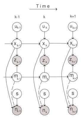
Figure 4: The dynamic Bayesian network representing the dependency between the random variables which feature in the described inference problem

Count measurement $n_{k}$ depends on the map $\mathbf{m}_{k}$, hence the likelihood of count measurement is formulated as $g_{1}(n_{k}|\mathbf{p}_{k},\mathbf{m}_{k},\mathbf{s})$. The searcher, however, does not know the map (it estimates it only partially as it travels through the search area) and hence we have introduced the approximate measurement model expressed by (4)-(6). The searcher will therefore process count observations $n_{k}$ using the likelihood function which is independent of $\mathbf{m}_{k}$, and denoted by $\tilde{g}_{1}(n_{k}|\mathbf{p}_{k},\mathbf{s})$, rather than $g_{1}(n_{k}|\mathbf{p}_{k},\mathbf{m}_{k},\mathbf{s})$. We indicate this fact by drawing the arrow from $\mathbf{m}_{k}$ to $n_{k}$ in Fig.4 by a dashed line.

The computation of the posterior PDF for a structured complex system such as the one shown in Fig.4 can be factorised and consequently made computationally and statistically more efficient. Technical details will be given in Sec.IV.

III-B Information driven motion control

After processing the measurements received at time $k-1$, the searcher needs to select the next control vector $\mathbf{u}_{k}$ which will change its position to $\mathbf{p}_{k}\sim p(\mathbf{p}_{k}|\mathbf{p}_{k-1},\mathbf{u}_{k})$. The problem of selecting $\mathbf{u}_{k}$ can be formulated as a partially-observed Markov decision process [20], whose elements are: (1) the set of admissible control vectors $\mathcal{U}_{k}$; (2) the current information state, expressed by the predicted PDF $p(\mathbf{y}_{k}|\mbox{\boldmath$\zeta$}_{1:k-1},\mathbf{u}_{1:k-1},\mathbf{u}_{k})$, where $\mathbf{u}_{k}\in\mathcal{U}_{k}$; (3) the reward function associated with each control $\mathbf{u}_{k}\in\mathcal{U}_{k}$. In the paper we adopt motion control based on a single step ahead strategy; this myopic approach is suboptimal in the presence of randomly missing links, but is computationally easier to implement and faster to run. The control vector is then selected as:

$$\mathbf{u}_{k}=\arg\max_{\mathbf{v}\in\mathcal{U}_{k}}\mathbb{E}\{\mathcal{D}(\mathbf{v},p(\mathbf{y}_{k}|\mbox{\boldmath$\zeta$}_{1:k-1},\mathbf{u}_{1:k-1},\mathbf{v}),\mbox{\boldmath$\zeta$}_{k}(\mathbf{v}))\}$$ (12)

where $\mathcal{D}(\mathbf{u},p,\mbox{\boldmath$\zeta$})$ is the reward function. Note that the reward depends on future measurement $\mbox{\boldmath$\zeta$}_{k}=[n_{k}\;\mathbf{z}_{k}^{\intercal}]^{\intercal}$, which would be acquired after control $\mathbf{u}\in\mathcal{U}_{k}$ had been applied. Since the decision has to be made before the actual control is applied, the expectation $\mathbb{E}$ is taken in (12) with respect to the prior measurements PDF.

Considering that the primary mission of the search is source localisation (map estimation is of secondary importance), the reward function at time $k$ is adopted as the information gain between: (1) the predicted PDF over the state subspace $(\mathbf{s},\mathbf{p}_{k})$ and (2) the updated PDF over $(\mathbf{s},\mathbf{p}_{k})$, using the count measurement $n_{k}$. The two distributions are denoted $\pi_{0}(\mathbf{s},\mathbf{p}_{k}|\mathbf{u}_{k})=p(\mathbf{s}|n_{1:k-1},\mathbf{u}_{1:k})p(\mathbf{p}_{k}|\mathbf{p}_{k-1},\mathbf{u}_{k})$ and $\pi_{1}(\mathbf{s},\mathbf{p}_{k}|n_{k},\mathbf{u}_{k})=\xi\,\tilde{g}_{1}(n_{k}|\mathbf{p}_{k},\mathbf{s})\,\pi_{0}(\mathbf{s},\mathbf{p}_{k}|\mathbf{u}_{k})$, respectively, where $\xi$ is a normalisation constant. The information gain between the two distributions is measured using the Bhattacharya distance [21]. The reward function is thus adopted as:

$$\mathcal{D}(\mathbf{u}_{k})=-2\log\int\sqrt{\pi_{1}(\mathbf{s},\mathbf{p}_{k}|n_{k},\mathbf{u}_{k})\cdot\pi_{0}(\mathbf{s},\mathbf{p}_{k}|\mathbf{u}_{k})}\;d\mathbf{s}\,d\mathbf{p}_{k}$$ (13)

where we dropped unnecessary arguments in notation for $\mathcal{D}$.

IV The search algorithm

The proposed search algorithm, formulated as a DBN with observer control, can be implemented efficiently as a Rao-Blackwellised particle filter (RBPF) [22] with sensor control. The idea of the RBPF is as follows. Suppose it is possible to divide the components of the hidden state vector $\mathbf{y}_{k}$ into two groups, $\mbox{\boldmath$\alpha$}_{k}$ and $\mbox{\boldmath$\beta$}_{k}$, such that the following two conditions are satisfied:

$$\text{{\bf C-1:}}\hskip 5.69054ptp(\mathbf{y}_{k}|\mathbf{y}_{k-1},\mathbf{u}_{k})=p(\mbox{\boldmath$\alpha$}_{k}|\mbox{\boldmath$\beta$}_{k-1:k},\mbox{\boldmath$\alpha$}_{k-1})\cdot p(\mbox{\boldmath$\beta$}_{k}|\mbox{\boldmath$\beta$}_{k-1},\mathbf{u}_{k})$$

C-2: the conditional posterior distribution $p(\mbox{\boldmath$\alpha$}_{k}|\leavevmode\nobreak\ \mbox{\boldmath$\beta$}_{0:k},\leavevmode\nobreak\ \mbox{\boldmath$\zeta$}_{1:k},\leavevmode\nobreak\ \mathbf{u}_{1:k})$ is analytically tractable.

Then we need only to estimate the posterior $p(\mbox{\boldmath$\beta$}_{0:k}|\mbox{\boldmath$\zeta$}_{1:k},\mathbf{u}_{1:k})$, meaning that we reduced the dimension of the space in which Monte Carlo estimation needs to be carried out, from $\text{dim}(\mathbf{y}_{k})$ to $\text{dim}(\mbox{\boldmath$\beta$}_{k})$. As argued in [22], this potentially improves computational and statistical efficiency of the particle filter.

In the described DBN, shown in Fig,4, in order to satisfy conditions C-1 and C-2, the state vector $\mathbf{y}_{k}$ can be partitioned as follows:

$$\mbox{\boldmath$\alpha$}_{k} =[\mathbf{m}_{k}^{\intercal}\;\;A]^{\intercal}$$ (14)

$$\mbox{\boldmath$\beta$}_{k} =[\mathbf{p}_{k}^{\intercal}\;\;X\;\;Y]^{\intercal}.$$ (15)

We are interested only in the filtering posterior density, which can now be factorised as follows:

$$p(\mbox{\boldmath$\alpha$}_{k} ,\mbox{\boldmath$\beta$}_{0:k}|\mbox{\boldmath$\zeta$}_{1:k},\mathbf{u}_{1:k})=$$

$$p(\mbox{\boldmath$\alpha$}_{k}|\mbox{\boldmath$\beta$}_{0:k},\mbox{\boldmath$\zeta$}_{1:k},\mathbf{u}_{1:k})\cdot p(\mbox{\boldmath$\beta$}_{0:k}|\mbox{\boldmath$\zeta$}_{1:k},\mathbf{u}_{1:k})$$ (16)

The PDF $p(\mbox{\boldmath$\beta$}_{0:k}|\mbox{\boldmath$\zeta$}_{1:k},\mathbf{u}_{1:k})$ is approximated by a random sample $\{\mbox{\boldmath$\beta$}_{0:k}^{(i)}\}_{i=1}^{N}$. Subsequently one can compute analytically (for each sample $\mbox{\boldmath$\beta$}_{0:k}^{(i)}$):

$$p(\mbox{\boldmath$\alpha$}_{k} |\mbox{\boldmath$\beta$}_{0:k}^{(i)},n_{1:k},\mathbf{z}_{1:k},\mathbf{u}_{1:k})=$$

$$p(\mathbf{m}_{k}|\mathbf{z}_{1:k},\mbox{\boldmath$\beta$}_{0:k}^{(i)})\cdot p(A|n_{1:k},\mbox{\boldmath$\beta$}_{0:k}^{(i)}),$$ (17)

where

• $p(\mathbf{m}_{k}|\mathbf{z}_{1:k},\mbox{\boldmath$\beta$}_{0:k}^{(i)})=\mathbf{q}_{k}$ is a vector of probabilities of existence for each link in the random grid and

• $p(A|n_{1:k},\mbox{\boldmath$\beta$}_{0:k}^{(i)})$ is approximated by a Gamma distribution with shape parameter $\eta_{k}$ and scale parameter $\theta_{k}$, i.e. $\mathcal{G}\left(A;\eta_{k},\theta_{k}\right)$.

Hence each particle corresponds to a set:

$$\left(\beta_{1:k}^{(i)},\mathbf{q}_{k},\eta_{k},\theta_{k}\right)$$ (18)

where $\mathbf{q}_{k},\eta_{k},\theta_{k}$ are the sufficient statistics of $p(\mbox{\boldmath$\alpha$}_{k}|\mbox{\boldmath$\beta$}_{0:k}^{(i)},n_{1:k},\mathbf{z}_{1:k},\mathbf{u}_{1:k})$. Keep in mind that $\mathbf{q}_{k},\eta_{k},\theta_{k}$ depend on a particular sequence (particle) $\beta_{0:k}^{(i)}$.

IV-A Recursive formulae for sufficient statistics

Let us first discuss the analytic recursive formula for the computation of $\mathbf{q}_{k}$, following the ideas of the grid-based SLAM [11]. Note that

$$\mathbf{q}_{k}= p(\mathbf{m}_{k}|\mathbf{z}_{1:k},\mbox{\boldmath$\beta$}_{0:k}^{(i)})=$$

$$\frac{g_{2}(\mathbf{z}_{k}|\mathbf{m}_{k},\mbox{\boldmath$\beta$}_{k}^{(i)})\,p(\mathbf{m}_{k}|\mathbf{z}_{1:k-1},\mbox{\boldmath$\beta$}_{0:k-1}^{(i)})}{\sum_{\mathbf{m}_{k}}g_{2}(\mathbf{z}_{k}|\mathbf{m}_{k},\mbox{\boldmath$\beta$}_{k}^{(i)})\,p(\mathbf{m}_{k}|\mathbf{z}_{1:k-1},\mbox{\boldmath$\beta$}_{0:k-1}^{(i)})}$$ (19)

where

$$p(\mathbf{m}_{k}| \mathbf{z}_{1:k-1},\mbox{\boldmath$\beta$}_{0:k-1}^{(i)})=$$

$$\sum_{\mathbf{m}_{k-1}}p(\mathbf{m}_{k}|\mathbf{m}_{k-1})\,p(\mathbf{m}_{k-1}|\mathbf{z}_{1:k-1},\mbox{\boldmath$\beta$}_{0:k-1}^{(i)})$$ (20)

The update of probability vector $\mathbf{q}_{k}$ is then carried out as follows. Recall from (15) that particle $\mbox{\boldmath$\beta$}_{k}^{(i)}$ specifies the location of the searcher at time $k$, $\mathbf{p}_{k}^{(i)}=[x_{k}^{(i)}\;\;y_{k}^{(i)}]^{\intercal}$. Each component of vector $\mathbf{z}_{k}$ is then an observation of existence of a primary or a secondary link from location $\mathbf{p}_{k}^{(i)}$. Let $q_{j,k-1}$ be a component of vector $\mathbf{q}_{k-1}$, denoting the posterior probability that link $\ell_{j}$ exists at time $k-1$, i.e. $q_{j,k-1}=p(m_{j,k-1}|\mathbf{z}_{1:k-1},\mbox{\boldmath$\beta$}_{0:k-1}^{(i)})$. Recall also that since the link statuses are assumed independent, then $\mathbf{q}_{k-1}=\prod_{j=1}^{L}q_{j,k-1}$. According to (20), link $j$ existence probability is predicted as:

$$q_{j,k|k-1}=p (m_{j,k}=1|m_{j,k-1}=0)(1-q_{j,k-1})+$$

$$\;\;p(m_{j,k}=1|m_{j.k-1}=1)q_{j,k-1}$$ (21)

Let $z$ be a component of vector $\mathbf{z}_{k}$ which refers to link $\ell_{j}$, according to the current position of the searcher, $\mathbf{p}_{k}^{(i)}$. Then based on (19) we update the link $j$ existence probability as:

$$q_{j,k}=\begin{cases}\frac{p_{d}\,q_{j,k|k-1}}{p_{d}\,q_{j,k|k-1}+p_{fa}(1-q_{j,k|k-1})}&\text{ if }z=1\\ &\\ \frac{(1-p_{d})\,q_{j,k|k-1}}{(1-p_{d})\,q_{j,k|k-1}+(1-p_{fa})(1-q_{j,k|k-1})}&\text{ if }z=0\end{cases}$$ (22)

where $p_{d}$ and $p_{fa}$, introduced in (8), are the elements of the appropriate detection $\Pi$ matrix (primary or secondary) of (8). Equations (19)-(22) can be summarised as:

$$\mathbf{q}_{k}=\psi(\mathbf{q}_{k-1},\mbox{\boldmath$\beta$}_{k}^{(i)},\mathbf{z}_{k})$$ (23)

Let us describe next the analytic recursion for the update of the parameters $\eta_{k}$ and $\theta_{k}$ of (18). At time $k-1$, the posterior of emission rate $A$ is modeled by a gamma distribution:

$$A|n_{1:k-1},\mbox{\boldmath$\beta$}_{0:k-1}^{(i)}\sim\mathcal{G}\left(A;\eta_{k-1},\theta_{k-1})\right).$$ (24)

Sensor 1 provides at time $k$ a count measurement $n_{k}$, which plays the key role in the update of parameters $\eta_{k-1}$ and $\theta_{k-1}$. Recall that the likelihood function of this measurement, $\tilde{g}_{1}(n_{k}|\mbox{\boldmath$\beta$}_{k}^{(i)},A)$ is a Poisson distribution with parameter (mean) $\lambda^{(i)}_{k-1}$, rather than $A$. Fortunately, $\lambda^{(i)}_{k-1}$ is linearly related to emission rate $A$, that is

$$\lambda^{(i)}_{k}=A\cdot c(\mbox{\boldmath$\beta$}_{k}^{(i)})$$

where the constant $c(\mbox{\boldmath$\beta$}_{k}^{(i)})$ is always positive and given by

$$c {}_{k}^{(i)}=-\frac{1}{2}\Big{(}2\log R_{0}+$$

$$\log\frac{(x_{k}^{(i)}-X^{(i)})^{2}+(y_{k}^{(i)}-Y^{(i)})^{2}}{(x_{k}^{(i)}Y^{(i)}-y_{k}^{(i)}X^{(i)})^{2}+(R_{0}^{2}-x_{k}^{(i)}X^{(i)}-y_{k}^{(i)}Y^{(i)})^{2}}\Big{)}.$$ (25)

with $X^{(i)}$ and $Y^{(i)}$, according to (15), being the components of particle $\mbox{\boldmath$\beta$}_{k}^{(i)}$.

In the proposed algorithm for the update of parameters $\eta_{k-1}$ and $\theta_{k-1}$ we use the following two properties of Gamma distribution:

1. Scaling property [23]: if $X\sim\mathcal{G}(\eta,\theta)$ then for any $c>0$, $cX\sim\mathcal{G}(\eta,c\theta)$.

2. Gamma distribution is the conjugate prior of Poisson distributions [24]: if $\lambda\sim\mathcal{G}(\eta,\theta)$ is a prior distribution and $n$ is a sample from the Poisson distribution with parameter $\lambda$, then the posterior is

   $$\lambda\sim\mathcal{G}(\eta+n,\theta/(1+\theta)).$$

Given $\mbox{\boldmath$\beta$}_{k}^{(i)}$ we can compute constant $c_{k}^{(i)}$ of (25) and express the prior distribution of $\lambda^{(i)}_{k-1}$ as:

$$\lambda^{(i)}_{k-1}|n_{1:k-1},\mbox{\boldmath$\beta$}_{0:k}^{(i)}\sim\mathcal{G}\left(\lambda;\eta_{k-1},\;c_{k}^{(i)}\cdot\theta_{k-1}\right)$$ (26)

Using measurement $n_{k}$ and the conjugate prior property, the posterior distribution is:

$$\lambda^{(i)}_{k}|n_{1:k},\mbox{\boldmath$\beta$}_{0:k}^{(i)}\sim\mathcal{G}\left(\lambda;\eta_{k-1}+n_{k},\;\frac{c_{k}^{(i)}\theta_{k-1}}{1+c_{k}^{(i)}\theta_{k-1}}\right)$$ (27)

Since we are after the updated parameters of Gamma distribution of $A$ (rather than $\lambda^{(i)}_{k}$), again using the scaling property we have:

$$A|n_{1:k},\mbox{\boldmath$\beta$}_{0:k}^{(i)}\sim\mathcal{G}\left(A;\eta_{k-1}+n_{k},\frac{\theta_{k-1}}{1+c_{k}^{(i)}\theta_{k-1}}\right)$$ (28)

We summarise from (24) and (28) the analytic expressions for the update of $\eta_{k}$ and $\theta_{k}$ :

$$\eta_{k} = \eta_{k-1}+n_{k}$$ (29)

$$\theta_{k} = \frac{\theta_{k-1}}{1+c_{k}^{(i)}\theta_{k-1}}$$ (30)

IV-B Importance weights

Recursive estimation of $p(\mbox{\boldmath$\beta$}_{0:k}|\mbox{\boldmath$\zeta$}_{1:k},\mathbf{u}_{1:k})$ is implemented using a particle filter. If we use the transitional prior as the proposal distribution. i.e.

$$q(\mbox{\boldmath$\beta$}_{0:k}| \mbox{\boldmath$\zeta$}_{1:k},\mathbf{u}_{1:k-1})=$$

$$p(\mbox{\boldmath$\beta$}_{k}|\mbox{\boldmath$\beta$}_{k-1},\mathbf{u}_{k})\,p(\mbox{\boldmath$\beta$}_{0:k-1}|\mbox{\boldmath$\zeta$}_{1:k-1},\mathbf{u}_{1:k-1})$$ (31)

the importance weights can be computed recursively as follows [22]:

$$w_{k}\propto p(\mbox{\boldmath$\zeta$}_{k}|\mbox{\boldmath$\zeta$}_{1:k-1},\mbox{\boldmath$\beta$}_{0:k})$$ (32)

For our problem expression (32) can be evaluated as:

$$w_{k} \propto \int p(\mbox{\boldmath$\zeta$}_{k},\mbox{\boldmath$\alpha$}_{k}|\mbox{\boldmath$\zeta$}_{1:k-1},\mbox{\boldmath$\beta$}_{0:k})\,d\mbox{\boldmath$\alpha$}_{k}$$ (34)

$$= \int\tilde{g}_{1}(n_{k}|A,\mbox{\boldmath$\beta$}_{k})\,p(A|n_{1:k-1},\mbox{\boldmath$\beta$}_{0:k-1})\,dA\times$$

$$\sum_{\mathbf{m}_{k}}g_{2}(\mathbf{z}_{k}|\mathbf{m}_{k},\mathbf{p}_{k})\,p(\mathbf{m}_{k}|\mathbf{z}_{1:k-1},\mbox{\boldmath$\beta$}_{0:k-1})$$

where $p(A|n_{1:k-1},\mbox{\boldmath$\beta$}_{0:k-1})$ is given by (24) and $p(\mathbf{m}_{k}|\mathbf{z}_{1:k-1},\mbox{\boldmath$\beta$}_{0:k-1})=\mathbf{q}_{k|k-1}$ by (20), i.e.

$$\mathbf{q}_{k|k-1}=\sum_{\mathbf{m}_{k-1}}p(\mathbf{m}_{k}|\mathbf{m}_{k-1})\,\mathbf{q}_{k-1}.$$

The components of vector $\mathbf{q}_{k|k-1}$, i.e. $q_{j,k|k-1}$, were specified by (21). The integral which features in (34) can also be computed analytically. This integral equals:

$$\mathcal{I} =\int\tilde{g}_{1}(n_{k}|A,\mbox{\boldmath$\beta$}_{k})\,p(A|n_{1:k-1},\mbox{\boldmath$\beta$}_{0:k-1})\,dA$$ (35)

$$=\int\mathcal{P}(n_{k};\lambda_{k}=c(\mbox{\boldmath$\beta$}_{k})\cdot A)\;\mathcal{G}(A;\eta_{k-1},\theta_{k-1})dA$$ (36)

where $\mathcal{P}(n;\lambda)$ is the Poisson distribution introduced in (4). Recall the explanation presented in Sec.IV-A about the update of the parameters of the Gamma distribution, summarised by (26)-(28). Effectively we have shown there that:

$$\mathcal{G} \left(A;\eta_{k-1}+n_{k},\frac{\theta_{k-1}}{1+c_{k}^{(i)}\theta_{k-1}}\right)=$$

$$\frac{\mathcal{P}(n_{k};\lambda_{k}=c(\mbox{\boldmath$\beta$}_{k})\cdot A)\;\mathcal{G}(A;\eta_{k-1},\theta_{k-1})}{\int\mathcal{P}(n_{k};\lambda_{k}=c(\mbox{\boldmath$\beta$}_{k})\cdot A)\;\mathcal{G}(A;\eta_{k-1},\theta_{k-1})dA}$$ (37)

where the integral in the denominator is $\mathcal{I}$, see (36). Hence, the integral can be expressed as:

$$\mathcal{I}=\frac{\mathcal{P}(n_{k}|\lambda_{k}=c(\mbox{\boldmath$\beta$}_{k})\cdot A)\;\mathcal{G}(A;\eta_{k-1},\theta_{k-1})}{\mathcal{G}(A;\eta_{k-1}+n_{k},\theta_{k-1}/(1+c(\mbox{\boldmath$\beta$}_{k})\theta_{k-1}))}$$ (38)

and is computed for an arbitrary chosen value of $A>0$. Based on (34), let us summarise the expression for an unnormalised importance weight as:

$$\tilde{w}_{k}=\varphi(\mbox{\boldmath$\beta$}_{k},\mathbf{q}_{k-1},\eta_{k-1},\theta_{k-1},n_{k},\mathbf{z}_{k})$$ (39)

Importance weights determine in a probabilistic manner which particles will survive (and possibly multiply) during the resampling step of the RBPF.

IV-C Information gain

Suppose the posterior distribution at time $k-1$, $p(\mathbf{y}_{k-1}|\mbox{\boldmath$\zeta$}_{1:k-1},\mathbf{u}_{1:k-1})$, is approximated by a set of particles:

$$\mathcal{Y}_{k-1}=\left\{\left(\mbox{\boldmath$\beta$}_{k-1}^{(i)},\mathbf{q}_{k-1}^{(i)},\eta_{k-1}^{(i)},\theta_{k-1}^{(i)}\right)\right\}_{i=1}^{N},$$ (40)

where random sample $\mbox{\boldmath$\beta$}^{(i)}_{k-1}$ consists of the searcher position $\mathbf{p}^{(i)}_{k-1}=[x_{k-1}^{(i)}\;\;y_{k-1}^{(i)}]^{\intercal}$ and the position of the source $\mathbf{p}^{(i)}_{s}=[X^{(i)}\;\;Y^{(i)}]^{\intercal}$, see (15). The weights of the particles in $\mathcal{Y}_{k-1}$ are equal, because sensor control is carried out after resampling, i.e. $w_{k-1}^{(i)}=1/N$, $i=1,\dots,N$.

The question is how to compute the information gain (13) for each $\mathbf{u}\in\mathcal{U}_{k}$, based on particles $\mathcal{Y}_{k-1}$. We adopt the ideal measurement approximation for this, that is, in hypothesizing the future count measurement (resulting from action $\mathbf{u}$), we assume: (1) action $\mathbf{u}$ will be carried out correctly, that is the transitional density $p(\mathbf{p}_{k}|\mathbf{p}_{k-1},\mathbf{u}_{k})$ will be replaced by deterministic mapping: $\mathbf{p}_{k}=\mathbf{p}_{k-1}+\mathbf{u}_{k}$, and (2) the measurement count will be equal to the mean of $\tilde{g}_{1}(n_{k}|A,\mbox{\boldmath$\beta$}_{k})$, that is $\lambda_{k}$ (rounded off to the nearest integer).

Since we are after the expected value of the gain, that is $\mathbb{E}\{\mathcal{D}(\mathbf{u})\}$, we will create an ensemble of “future ideal measurements” $\{n_{k}^{(j)}\}_{j=1}^{M}$. Expectation is then approximated by a sample mean, i.e.

$$\mathbb{E}\{\mathcal{D}(\mathbf{u})\}\approx\frac{1}{M}\sum_{j=1}^{M}\mathcal{D}^{(j)}(\mathbf{u})$$

where $\mathcal{D}^{(j)}(\mathbf{u})$ was computed using $n_{k}^{(j)}$.

The ensemble of “future ideal measurements” $\{n_{k}^{(j)}\}_{j=1}^{M}$ is created as follows. For each action $\mathbf{u}$, choose at random a set of $M$ particle indices $i_{j}\in\{1,\dots,N\}$, $j=1,\dots,M$. Action $\mathbf{u}$ is then expected to move the searcher to location $\mathbf{p}_{k}^{(i_{j})}=\mathbf{p}_{k-1}^{(i_{j})}+\mathbf{u}$. Then a “future ideal measurement” is $n_{k}^{(j)}=\lfloor A^{(i_{j})}\cdot c^{(i_{j})}\rceil$, where $c^{(i_{j})}$ as a function of $\mathbf{p}_{k}^{(i_{j})},\mathbf{p}_{s}^{(i_{j})}$ was defined by (25), $A^{(i_{j})}\sim\mathcal{G}(A;\eta_{k-1},\theta_{k-1})$, and $\lfloor\cdot\rceil$ denotes the nearest integer function.

It remains to explain how to compute the gain $D^{(j)}(\mathbf{u})$ based on $n_{k}^{(j)}$. Distribution $\pi_{0}(\mathbf{s},\mathbf{p}_{k}|\mathbf{u}_{k})$, which features in (13), can be approximated using the particle set $\mathcal{Y}_{k-1}$ as follows:

$$\pi_{o}(\mathbf{s},\mathbf{p}_{k},\mathbf{u})\approx\mathcal{G}(A;\eta_{k-1},\theta_{k-1})\sum_{i=1}^{N}w^{(i)}_{k-1}\delta(\mathbf{p}_{s}-\mathbf{p}_{s}^{(i)},\mathbf{p}_{k}-\mathbf{p}_{k}^{(i)})$$ (41)

where $\mathbf{p}_{k}^{(i)}\sim p(\mathbf{p}_{k}|\mathbf{p}_{k-1}^{(i)},\mathbf{u})$. The updated distribution is

$$\pi_{1}(\mathbf{s},\mathbf{p}_{k} |\mathbf{u},n_{k}^{(j)})=$$

$$\frac{\tilde{g}_{1}(n_{k}^{(j)}|\mathbf{p}_{k},\mathbf{p}_{s},A)\pi_{o}(\mathbf{s},\mathbf{p}_{k}|\mathbf{u})}{\int\tilde{g}_{1}(n_{k}^{(j)}|\mathbf{p}_{k},\mathbf{p}_{s},A)\pi_{o}(\mathbf{s},\mathbf{p}_{k}|\mathbf{u})d\mathbf{s}d\mathbf{p}_{k}}.$$ (42)

Substitution of (41) and (42) into (13) leads to:

$$\mathcal{D}^{(j)}(\mathbf{u})\approx-2\log\frac{\sum_{i=1}^{N}w_{k-1}^{(i)}\mathcal{J}^{(i)}(n_{k}^{(j)})}{\left[\sum_{i=1}^{N}w^{(i)}_{k-1}\mathcal{I}^{(i)}(n_{k}^{(j)})\right]^{1/2}}$$ (43)

where $\mathcal{I}^{(i)}(n_{k})$ is computed via (38) and

$$\mathcal{J}^{(i)}(n_{k})=\int \left[\mathcal{P}(n_{k};\lambda^{(i)}_{k}=c(\mbox{\boldmath$\beta$}^{(i)}_{k})A)\right]^{1/2}\times$$

$$\hskip 11.38109pt\mathcal{G}(A;\eta^{(i)}_{k-1},\theta^{(i)}_{k-1})dA$$ (44)

Integral (44) can be evaluated numerically.

IV-D Implementation

The pseudo-code of one cycle of the search algorithm is presented in Algorithm 1. The input consists of the particle set $\mathcal{Y}_{k-1}$, defined by (40). Selection of the control vector $\mathbf{u}_{k}$ (line 2 of Algorithm 1) is described in Algorithm 2.

Explanation of the steps in Algorithm 1 are described first. Estimation of the state vector via the RBPF is carried out in lines 4-18. According to (15), random vector $\mbox{\boldmath$\beta$}^{(i)}_{k-1}$ consists of $\mathbf{p}_{k-1}^{(i)}$, $X^{(i)}$ and $Y^{(i)}$. Since the source location, $(X^{(i)},Y^{(i)})$, is static, only the component $\mathbf{p}_{k-1}^{(i)}$ is propagated to future time $k$ in line 6. In line 7, equation (39) is applied to compute the unnormalised weights of each particle. The map, represented by the probability of existence of each link, is updated in line 8, based on the expression (23). The parameters of Gamma distribution are update in lines 9-11. The weights assigned to each quadruple $(\mbox{\boldmath$\beta$}_{k}^{(i)},\mathbf{q}_{k}^{(i)},\eta_{k}^{(i)},\theta_{k}^{(i)})$ are normalised in line 14. Resampling of particles is carried out in lines 15-18. The particles for source position $\mathbf{p}_{s}^{(i)}$ are not restricted to the grid nodes and after the resampling step, their diversity is improved by regularisation [25]. Finally, the output is the particle set $\mathcal{Y}_{k}$.

Algorithm 1 The searcher algorithm

1:Input: $\mathcal{Y}_{k-1}$

2:Run Algorithm 2 to select the control vector $\mathbf{u}_{k}$

3:Apply control $\mathbf{u}_{k}$ and collect measurements $\mathbf{z}_{k}$, $n_{k}$

4:$\mathcal{\overline{Y}}_{k}=\emptyset$; $\mathcal{Y}_{k}=\emptyset$

5:for $i=1,\dots,N$ do

6:    Draw $\mathbf{p}_{k}^{(i)}\sim p(\mathbf{p}_{k}|\mathbf{p}_{k-1}^{(i)},\mathbf{u}_{k})$

7:    $\tilde{w}_{k}^{(i)}=\varphi(\mbox{\boldmath$\beta$}^{(i)}_{k},\mathbf{q}_{k-1}^{(i)},\eta_{k-1}^{(i)},\theta_{k-1}^{(i)},n_{k},\mathbf{z}_{k})$

8:    $\mathbf{q}_{k}^{(i)}=\psi(\mathbf{q}^{(i)}_{k-1},\mbox{\boldmath$\beta$}_{k}^{(i)},\mathbf{z}_{k})$

9:    $\eta_{k}^{(i)}=\eta_{k-1}^{(i)}+n_{k}$

10:    Compute constant $c_{k}^{(i)}$ as a function of $\mbox{\boldmath$\beta$}_{k}^{(i)}$ using (25)

11:    $\theta_{k}^{(i)}=\theta_{k-1}^{(i)}/(1+c_{k}^{(i)}\theta_{k-1}^{(i)})$

12:    $\mathcal{\overline{Y}}_{k}=\mathcal{\overline{Y}}_{k}\cup\{(\mbox{\boldmath$\beta$}_{k}^{(i)},\mathbf{q}_{k}^{(i)},\eta_{k}^{(i)},\theta_{k}^{(i)})\}$

13:end for

14:$w_{k}^{(i)}=\tilde{w}_{k}^{(i)}/\sum_{j=1}^{N}\tilde{w}_{k}^{(j)}$, for $i=1,\dots,N$

15:for $i=1,\dots,N$ do

16:    Select index $j^{i}\in\{1,\dots,N\}$ with probability $w_{k}^{(i)}$

17:    $\mathcal{Y}_{k}=\mathcal{Y}_{k}\cup\{(\mbox{\boldmath$\beta$}_{k}^{(j_{i})},\mathbf{q}_{k}^{(j_{i})},\eta_{k}^{(j_{i})},\theta_{k}^{(j_{i})})\}$

18:end for

19:Output: $\mathcal{Y}_{k}$

The selection of a control vector, described by Algorithm 2, starts with postulating the set $\mathcal{U}_{k}$ in line 2. For every $\mathbf{u}\in\mathcal{U}_{k}$, the algorithm anticipates $j=1,\dots,M$ future measurements $n_{k}^{(j)}$ (line 9) and accordingly computes a sample of the reward $\mathcal{D}^{(j)}(\mathbf{u})$ (line 14). The expected reward is then a sample mean (line 16). Finally the optimal one-step ahead control is selected in line 18.

It has been observed in simulations that one step ahead control can sometimes lead to situations where the observer position switches eternally between two or three nodes of the lattice. In order to overcome this problem, we adopt a heuristic as follows: if a node has been visited in the last 10 search steps more than 3 times, the next motion control vector is selected at random. While a multi-step ahead searcher control would be preferable than adopted heuristic, it would also be computationally more demanding. Multi-step ahead searcher control remains to be explored in future work.

Algorithm 2 Selection of control vector

1:Input: $\mathcal{Y}_{k-1}$

2:Create the set of admissible controls $\mathcal{U}_{k}=\{\cdot,\uparrow,\rightarrow,\downarrow,\leftarrow\}$

3:for every $\mathbf{u}\in\mathcal{U}_{k}$ do

4:    for $j=1,\dots,M$ do

5:         Choose at random particle index $i_{j}\in\{1,\dots,N\}$

6:         $\mathbf{p}_{k}^{(i_{j})}=\mathbf{p}^{(i_{j})}_{k-1}+\mathbf{u}$;

7:         Compute $c^{(i_{j})}_{k}$ using $\mathbf{p}_{k}^{(i_{j})}$ and $\mathbf{p}_{s}^{(i_{j})}$ via (25)

8:         Adopt $A^{(i_{j})}=\eta^{(i_{j})}_{k-1}\cdot\theta^{(i_{j})}_{k-1}$

9:         $n_{k}^{(j)}=\lfloor A^{(i_{j})}\cdot c^{(i_{j})}_{k}\rceil$

10:         for $i=1,\dots,N$ do

11:             Compute $\mathcal{I}^{(i)}(n_{k}^{(j)})$ via (38)

12:             Compute $\mathcal{J}^{(i)}(n_{k}^{(j)})$ via (44)

13:         end for

14:         Compute $\mathcal{D}^{(j)}(\mathbf{u})$ using (43)

15:    end for

16:    Estimate $\mathbb{E}\{\mathcal{D}(\mathbf{u})\}$ as a sample mean of $\{\mathcal{D}^{(j)}(\mathbf{u})\}_{j=1}^{M}$

17:end for

18:Select control vector $\mathbf{u}_{k}\in\mathcal{U}_{k}$ using (12)

V Numerical results

V-A An illustrative run

We applied the described search algorithm to the search area modelled by the random grid shown in Fig.2. Prior knowledge available to the searcher is illustrated by Fig.1: the radius of the search area is $R_{0}=9$; the centre is $\mathbf{c}=(0,0)$ and the total number of potential links in the complete grid modelling the search area is $L=572$. The parameters of the emitting source to be estimated are: $X=0$, $Y=7$ and $A_{0}=12$. The searcher initial position is $\mathbf{p}_{0}=(9,-4)$.

Dynamic model $p(\mathbf{m}_{k}|\mathbf{m}_{k-1})$ is is a $2\times 2$ transitional probability matrix with diagonal and off-diagonal elements $0.999$ and $0.001$, respectively. Dynamic model $p(\mathbf{p}_{k}|\mathbf{p}_{k-1},\mathbf{u}_{k})$ can be expressed as:

$$p(\mathbf{p}_{k}|\mathbf{p}_{k-1},\mathbf{u}_{k})= (1-p_{e})\delta(\mathbf{p}_{k}-\mathbf{p}_{k-1}+\mathbf{u}_{k})+$$

$$\sum_{\mathbf{v}\in\mathcal{U}_{k}\setminus\mathbf{u}_{k}}\frac{p_{e}}{|\mathcal{U}_{k}|-1}\delta(\mathbf{p}_{k}-\mathbf{p}_{k-1}+\mathbf{v})$$ (45)

where in simulations we used the value $p_{e}=0.04$.

The parameters of detection matrices, which define the likelihood function $g_{2}(\mathbf{z}_{k}|\mathbf{p}_{k},\mathbf{m}_{k})$, are as follows: for primary observable links, $p_{d}=1$ and $p_{fa}=0$; for secondary observable links $p_{d}=0.8$ and $p_{fa}=0.1$.

The RBPF used $N=4000$ particles with $M=400$ samples used in the averaging of information gain. The particle set $\mathcal{Y}_{0}$ at initial time is created as follows: $\mathbf{p}^{(i)}_{0}=\mathbf{p}_{0}$, for all $i=1,\dots,N$ particles; the source location vector is drawn from a uniform distribution over a circle with centre $\mathbf{c}$ and radius $R_{0}$, i.e. $\mathbf{p}^{(i)}_{s}\sim\mathcal{U}_{\text{Circle}(\mathbf{c},R_{0})}(\mathbf{p}_{s})$; link existence probabilities are set to $q_{j,0}=0.5$, for all $j=1,\dots,L$ links; finally, the parameters of initial Gamma distribution $\mathcal{G}(A;\eta_{0},\theta_{0})$ were selected as $\eta_{0}=15$ and $\theta_{0}=1$.

We terminate the search algorithm when the searcher steps on the source. At this point we compare the true source location with the current estimate of the posterior distribution of the searcher position, approximated by particles $\{\mathbf{p}_{k}^{(i)}\}_{i=1}^{N}$. If the true source position is contained in the support defined by $\{\mathbf{p}_{k}^{(i)}\}_{i=1}^{N}$, the search is considered successful.

Fig. 5 illustrates a typical run of the search algorithm. The true path of the searcher on this run is shown in Fig.5.(a). It took the searcher $53$ time steps to reach the source. During the search, the motion control vector failed to execute correctly on two occasions. The final estimate of the map (i.e of existing links of the square lattice) is shown in Fig.5.(b). This figure shows only the links whose probability of existence is higher than $0.6$. The blue circles in Fig.5.(b) indicate the posterior distribution of the searcher final position. Its true position, which is the same as the source position, is included in the support of this posterior, meaning that the search was successful. Moreover, on this occasion, the MAP estimate of the searcher final position coincides with the truth. Fig.5.(c) shows the measured values of the count number $n_{k}$ along the path. As we discussed in introduction, the measurements are sporadic, especially in the beginning, when the distance between the searcher and the source is large: among the first ten count measurements, only three indicated a non-zero tracer concentration.

     

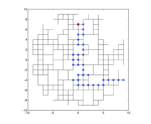
(a)

     

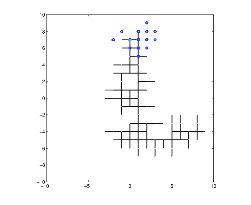
(b)

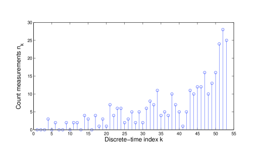
(c)

Figure 5: An illustration of a single run of the search algorithm: (a) The true path of the searcher (blue circles); (b) The final estimate of the map (existing links) and the searcher position; (c) measured counts $n_{k}$ over time

An avi video file, illustrating a single run of the algorithm, is supplied with the submission of this paper.

V-B Monte Carlo runs

The average performance of the search algorithm in the described scenario has been assessed via Monte Carlo runs. If the search on a particular run was successful, its corresponding search time is used in averaging. A run is declared unsuccessful if the source has not been found after $k=100$ discrete-time steps. We also keep the statistics on the success rate of the search. The results obtained via averaging over 100 Monte Carlo runs are presented in Table I for three different locations of the source, i.e. $(X,Y)=(0,7),(0,1),(2,-5)$. The three locations correspond to the shortest path distances (from the searcher initial position $\mathbf{p}_{0}=(9,-4)$ to the source) of $20$, $14$ and $8$ unit lengths, respectively. All other parameters were the same as described above for the illustrative run. As expected, the results in Table I indicate that the search is quicker and more reliable (i.e. with a higher success rate) for a source which is closer to the searcher initial position.

Table I: The average performance of the search algorithm: different source locations, $A_{0}=12$

Source	Shortest	Number of	Success
location	path length	search steps	rate [%]
$(0,7)$	$20$	$42.1$	$94$
$(0,1)$	$14$	$34.0$	$95$
$(2,-5)$	$8$	$28.8$	$99$

Table II presents the results for a source at location $(0,7)$ but with three different values of the source release-rate, i.e. $A_{0}=8,12,16$. The results indicate that the search is quicker for a source characterised by a higher release rate. The explanation of this trend is as follows. Initially, when the searcher is far from the source, its measurements of tracer concentration are very small, typically zero, hence uninformative. During this phase of the search, the searcher effectively moves according to a ‘diffusive’ (or random walk) model, which is slower that the so-called ’ballistic’ movement associated with information driven search [2]. The random walk phase is longer for a weaker source, which contributes to the overall longer search time in this case. As a specific numerical example, we have also validated that a purely random search never manages to find the source at $(0,7)$ in the given time-frame of $100$ discrete-time steps.

Table II: The average performance of the search algorithm: different source release-rates, source location $0,7)$

Release	Number of	Success
rate $A_{0}$	search steps	rate [%]
$8$	$49.5$	$78$
$12$	$42.1$	$94$
$16$	$38.2$	$93$

VI Summary

The paper considers a very difficult problem of autonomous search for a diffusive point source of tracer in an environment whose structure is unknown. Sequential estimation and motion control are carried out in highly uncertain circumstances with the state space including, in addition to the source parameters, the map of the search area and the searcher position within the map. The paper develops mathematical models of measurements, it formulates the sequential Bayesian solution (in the form of a Rao-Blackwellised particle filter) and proposes an information driven motion control of the searcher. The numerical results demonstrate the concept, indicating high success-rates in comparison with random walk.

There are many areas for further research and improvements of the concepts introduces in this paper. One direction is to explore the potential benefits of analytical results available from the percolation theory in carrying out olfactory search. Another is to investigate more efficient particle filters for source parameter estimation (being a deterministic part of the state space). Finally, the search strategies based on multiple steps ahead (rather than myopic search) are expected to improve the performance in a domain with obstacles.

An approximate model of mean concentration, independent of the grid structure, was introduced in Sec.II-C. This model is a solution of the Laplace equation (1) for a circular search area in the absence of obstacles, with a boundary condition $\theta(r=R_{0})=0$, but using different values of parameters. More specifically, the obstacles in the search area are incorporated in this model via homogenization (volume/ensemble averaging) of the diffusion equation (similar to the effective media approach [26], [27]), so that (1) is replaced with

$$D\;\Delta\langle\theta\rangle=A_{0}\delta(x-X,y-Y),$$ (46)

where $D$ is the re-scaled diffusivity that accounts for such a homogenization, and $\langle\theta\rangle$ is the time/ensemble averaged tracer concentration. The new (often called effective) diffusivity $D$ is related to ’unobstructed’ diffusivity $D_{0}$ of (1) via the formula $D=f_{c}D_{0}$. The scaling parameter $0\leq f_{c}\leq 1$ (known as tortuosity [14], [28]) describes the effect of obstacles (their shape and packing density [14], [27]). According to (46), the decrease of the effective diffusivity of the tracer due to the presence of obstacles has the same effect as an appropriate increase of source release-rate (i.e. $A=A_{0}/f_{c}$), with unchanged diffusivity in (46) (i.e. $D=D_{0}$), where parameters $D_{0},A_{0}$ correspond to their values in an unobstructed space, see (1). We arrive at a conclusion that the effect of obstacles can be approximately incorporated with imprecision (overestimation) of the source release-rate, without any effect on the source position. Since the main goal of the search algorithm is to find the source, then such inaccuracy in release-rate estimation becomes irrelevant for the performance of the algorithm. This means that as the first approximation for adopted measurements model we can still use (46) with known diffusivity $D=D_{0}$ and some unknown $A$. Estimation of $A_{0}$ (if required) can be implemented retrospectively based on a theoretical model for $f_{c}$ [28]). For the lattice models an expression for $f_{c}$ can be derived analytically by employing the framework of percolation theory, resulting in the expression $f_{c}=(1-p/p_{c})^{\alpha}$, where $p_{c}=1/2$ (percolation threshold on square lattice), $p$ is the fraction of missing links in the incomplete square lattice and $\alpha=1.30$ [13], [14]. If the number of missing links is small, we can adopt approximation $f_{c}\approx 1$ and $A\approx A_{0}$.

In line with the above comments we will use (46) as a foundation for the measurements model that is independent of the structure of the search domain. The solution of (46) for a tracer source located at the center of circle ($X=Y=0$), is given by [29]:

$$\langle\theta\rangle=\frac{A}{2}\log[(zz^{*})/R^{2}_{0}],$$ (47)

where $z=x+iy$ is the complex coordinate and $z^{*}$ is its complex-conjugate. To find the solution for configurations other than the circular domain with the source in the centre, we employ the property of conformal invariance of the Laplace equation [29]. We illustrate this method with a source placed inside the circular domain, but away from its centre (that is at coordinates $(X,Y)$ s.t. $\sqrt{X^{2}+Y^{2}}<R_{0}$). If we can find a conformal transformation $\omega(z)$ that maps an arbitrary position of the source $(X,Y)$ back to the center of the circular domain, then we can still use the solution (47), but with the substitution $z\rightarrow\omega(z)$. Therefore, for an arbitrary position of the source inside the search area $\sqrt{X^{2}+Y^{2}}<R_{0}$ we can write

$$\langle\theta\rangle=(\kappa/2)\log[(ww^{*})/R^{2}_{0}].$$ (48)

The required conformal transformation is the well-known Möbius map (see [29])

$$w(z)=\frac{R_{0}(z-Z)}{ZZ^{*}-R^{2}_{0}},$$ (49)

where $Z=X+iY$. After straightforward calculations we arrive at the solution given by (5) and (6).

We point out that the model is not restricted to a circular search area. According to the theory of analytical functions, a conformal mapping to the circle always exists for arbitrary simply connected domain, and therefore can be computed analytically or numerically [29].

References

- [1] G. M. Viswanathan, V. Afanasyev, S. V. Buldyrev, E. J. Murphy, P. A. Prince, and H. E. Satnley, “Levy fligh search patterns of wandering albatrosses,” Nature, vol. 381, pp. 413–415, 1996.
- [2] O. Bénichou, C. Loverdo, M. Moreau, and R. Voituriez, “Intermittent search strategies,” Rev. Mod. Phys., vol. 83, pp. 81–129, Mar 2011.
- [3] A. M. Hein and S. A. McKinley, “Sensing and decision-making in random search,” PNAS, July 2012.
- [4] J. A. Farrell, S. Pang, and W. Li, “Plume mapping via hidden Markov models,” IEEE Trans. Systems, Man, Cybernetics - Part B: Cybernetics, vol. 33, no. 6, pp. 850–863, 2003.
- [5] W. Li, J. A. Farrell, S. Pang, and R. M. Arrieta, “Moth-inspired chemical plume tracking on an autonomous underwater vehicle,” IEEE Trans Robotics, vol. 22, no. 2, pp. 292–307, 2006.
- [6] J. Oyekan and H. Hu, “A novel bio-controller for localizing pollution sources in a medium peclet environment,” Journal of Bionic Engineering, vol. 7, no. 4, pp. 345–353, 2010.
- [7] H. Ishida, G. Nakayama, T. Nakamoto, and T. Morizumi, “Controlling a gas/odor plume tracking robot based on transient responses of gas sensors,” IEEE Sensors Journals, vol. 5, no. 3, pp. 537–545, 2005.
- [8] M. Vergassola, E. Villermaux, and B. I. Shraiman, “‘infotaxis’ as a strategy for searching without gradients,” Nature, vol. 445, no. 25, pp. 406–409, 2007.
- [9] G. L. Iacono, “A comparison of different searching strategies to locate sources of odor in turbulent flows,” Adaptive Behavior, vol. 18, no. 2, pp. 155–170, 2010.
- [10] B. Ristic, M. Morelande, and A. Gunatilaka, “Information driven search for point sources of gamma radiation,” Signal Processing, vol. 90, pp. 1225–1239, 2010.
- [11] S. Thrun, W. Burgard, and D. Fox, Probabilistic Robotics. MIT Press, 2005.
- [12] A. Marjovi and L. Marques, “Multi-robot olfactory search in structured environment,” Robotics and Autonomous Systems, vol. 59, pp. 867–881, 2011.
- [13] D. ben Avraham and S. Havlin, Diffusion and reaction in fractals and disordered systems. Cambridge University Press, 2000.
- [14] S. Torquato, Heterogeneous materials. Springer, 2002.
- [15] J. G. Kemeny and J. L. Snell, Finite Markov chains. New York: Van Nostrand, 1960.
- [16] A. P. S. Selvadurai, Partial differential equations in Mechanics 1. Springer, 2000.
- [17] R. Burioni and D. Cassi, “Random walks on graphs: ideas, techniques and results,” Journal of Physics A: Mathematical and General, vol. 38, no. 8, p. R45, 2005.
- [18] A. Doucet, J. F. G. de Freitas, and N. J. Gordon, Eds., Sequential Monte Carlo Methods in Practice. Springer, 2001.
- [19] T. Dean and K. Kanazawa, “A model for reasoning about persistence and causation,” Computational intelligence, vol. 5, no. 2, pp. 142–150, 1989.
- [20] E. Chong, C. Kreucher, and A. Hero, “POMDP approximation using simulation and heuristics,” in Foundations and Applications of Sensor Management, A. Hero, D. Castanon, D. Cochran, and K. Kastella, Eds. Springer, 2008, ch. 8.
- [21] T. Kailath, “The divergence and Bhattacharyya distance measures in signal selection,” IEEE Trans. Communic. Technology, vol. 15, no. 1, pp. 52–60, 1967.
- [22] A. Doucet, N. de Freitas, K. P. Murphy, and S. J. Russell, “Rao-Blackwellised particle filtering for dynamic Bayesian networks,” in Proceedings of the 16th Conference on Uncertainty in Artificial Intelligence, 2000, pp. 176–183.
- [23] “Gamma-distribution,” in Encyclopedia of mathematics, M. Hazewinkel, Ed. Springer, 2001.
- [24] A. Gelman, J. B. Carlin, H. S. Stern, and D. B. Rubin, Bayesian data analysis, 2nd ed. CRC Press, 2003.
- [25] B. Ristic, S. Arulampalam, and N. Gordon, Beyond the Kalman filter: Particle filters for tracking applications. Artech House, 2004.
- [26] C. Nicholson, “Diffusion and related transport mechanisms in brain tissue,” Reports on progress in physics, vol. 64, pp. 815–884, 2001.
- [27] I. L. Novak, P. Kraikivski, and B. M. Slepchenko, “Diffusion in cytoplasm: Effects of excluded volume due to internal membranes and cytoskeletal structures,” Biophysical journal, vol. 97, pp. 758–767, 2009.
- [28] L. Pisani, “Simple expression for the tortuosity of porous media,” Transport in Porous Media, vol. 88, no. 2, pp. 193–203, 2011.
- [29] A. Prosperetti, Advanced mathematics for applications. Cambridge University Press, 2011.