Variational Data Assimilation via Sparse Regularization

Abstract

This paper studies the role of sparse regularization in a properly chosen basis for variational data assimilation (VDA) problems. Specifically, it focuses on data assimilation of noisy and down-sampled observations while the state variable of interest exhibits sparsity in the real or transformed domain. We show that in the presence of sparsity, the $\ell_{1}$-norm regularization produces more accurate and stable solutions than the classic data assimilation methods. To motivate further developments of the proposed methodology, assimilation experiments are conducted in the wavelet and spectral domain using the linear advection-diffusion equation.

1 Introduction

Environmental prediction models are initial value problems and their forecast skills highly depend on the quality of their initialization. Data assimilation (DA) seeks the best estimate of the initial condition of a (numerical) model, given observations and physical constraints coming from the underlying dynamics [see, Daley, 1993; Kalnay, 2003]. This important problem is typically addressed by two major classes of methodologies, namely sequential and variational methods [Ide et al., 1997]. The sequential methods are typically built on the theory of mathematical filtering and recursive weighted least-squares [Ghil et al., 1981; Ghil, 1989; Ghil and Malanotte-Rizzoli, 1991; Evensen, 1994a; Anderson, 2001; Moradkhani et al., 2005; Zhou et al., 2006; van Leeuwen, 2010, among others], while the variational methods are mainly rooted in the theories of constrained mathematical optimization and batch mode weighted least-squares (WLS) [e.g., Sasaki, 1970; Lorenc, 1986, 1988; Courtier and Talagrand, 1990; Zupanski, 1993, among others].

Although, recently the sequential methods have received a great deal of attention, the variational methods are still central to the operational weather forecasting systems. Classic formulation of the variational data assimilation (VDA) typically amounts to defining a (constrained) weighted least-squares penalty function whose optimal solution is the best estimate of the initial condition, the so-called analysis state. This penalty function typically encodes the weighted sum of the costs associated with the distance of the unknown true state to the available observations and previous model forecast, the so-called background state. Indeed, the penalty function enforces the solution to be close enough to both observations and background state in the weighted mean squared sense, while the weights are characterized by the observations and the background error covariance matrices. On the other hand, the constraints typically enforce the analysis to follow the underlying prognostic equations in a weak or strong sense [see, Sasaki, 1970; Daley, 1993, p.369]. Typically, when we constrain the analysis only to the available observations and the background state at every instant of time, the variational data assimilation problem is called 3D-Var [e.g., Lorenc, 1986; Parrish and Derber, 1992; Lorenc et al., 2000; Kleist et al., 2009]. On the other hand, when the analysis is also constrained to the underlying dynamics and available observations in a window of time, the problem is called 4D-Var [e.g., Zupanski, 1993; Rabier et al., 2000; Rawlins et al., 2007].

Inspired by the theories of smoothing spline and kriging interpolation in geostatistics, the first signs of using regularization in variational data assimilation trace back to the work by Wahba and Wendelberger [1980] and Lorenc [1986], where the motivation was to impose smoothness over the class of twice differentiable analysis states. More recently, Johnson et al. [2005b] argued that, in the classic VDA problem, the sum of the squared or $\ell_{2}$-norm of the weighted background error resembles the Tikhonov regularization [Tikhonov et al., 1977]. Specifically, by the well-known connections between the Tikhonov regularization and spectral filtering via singular value decomposition (SVD) [e.g., see Hansen, 1998; Golub et al., 1999; Hansen et al., 2006], a new insight was provided into the interpretation and the stabilizing role of the background state on the solution of the classic VDA problem [see, Johnson et al., 2005a]. Instead of using the $\ell_{2}$-norm of the background error, Freitag et al. [2010] and Budd et al. [2011] suggested to modify the classic VDA cost function using the sum of the absolute values or $\ell_{1}$-norm of the weighted background error. This assumption requires to statistically assume that the background error is heavy tailed and can be well approximated by the family of Laplace densities [e.g., Tibshirani, 1996; Lewicki and Sejnowski, 2000]. For data assimilation of sharp atmospheric fronts, Freitag et al. [2012] kept the classic VDA cost function while further proposed to regularize the analysis state by constraining the $\ell_{1}$-norm of its derivative coefficients. Ebtehaj and Foufoula-Georgiou [2013] also used Huber-norm regularization to assimilate noisy and low-resolution observations into the dynamics of the heat equation.

In this study, we extend the previous studies [e.g., Freitag et al., 2012; Ebtehaj and Foufoula-Georgiou, 2013] in regularized variational data assimilation (RVDA) by: (a) proposing a generalized regularization framework for assimilating low-resolution and noisy observations while the initial state of interest exhibits sparse representation in an appropriately chosen basis (i.e., wavelet, discrete cosine transform); (b) demonstrating the promise of the methodology in an assimilation example using advection-diffusion dynamics with different error structure; and (c) proposing an efficient solution method for large-scale data assimilation problems.

The concept of sparsity plays a central role in this paper. By definition, a state of interest is sparse in a pre-selected basis, if the number of non-zero elements of its expansion coefficients in that basis (e.g., wavelet coefficients) is significantly smaller than the overall dimension of the state in the observational space. Here, we show that if sparsity in a pre-selected basis holds, this prior information can serve to improve the accuracy and stability of data assimilation problems. To this end, using prototype studies, different initial conditions are selected, which are sparse under the wavelet and spectral discrete cosine transformation (DCT). The promise of the $\ell_{1}$-norm RVDA is demonstrated via assimilating down-sampled and noisy observations in a 4D-Var setting by strongly constraining the solution to the governing advection-diffusion equation. In a broader context, we delineate the roadmap and explain how we may exploit sparsity, while the underlying dynamics and observation operator might be nonlinear. Particular attention is given to explain Monte Carlo driven approaches that can incorporate a sparse prior in the context of ensemble data assimilation.

Section 2 reviews the classic variational data assimilation problem. In Section 3, we discuss the concept of sparsity and its relationship with $\ell_{1}$-norm regularization in the context of VDA problems. Results of the proposed framework and comparisons with classic methods are presented in Section 4. Section 5, is devoted to conclusions and ideas for future research, mainly focusing on the use of ensemble-based approaches to address sparse promoting VDA in nonlinear dynamics. Algorithmic details and derivations are presented in Appendix A.

2 Classic Variational Data Assimilation

At the time of model initialization $t_{0}$, the goal of data assimilation can be stated as that of obtaining the analysis state as the best estimate of the true initial state, given noisy and low-resolution observations and the erroneous background state, while the analysis needs to consistent with the underlying model dynamics. The background state in VDA is often considered to be the previous-time forecast provided by the prognostic model. By solving the VDA problem, the analysis is then being used as the initial condition of the underlying model to forecast the next time step and so on. In the following, we assume that the unknown true state of interest at the initial time $t_{0}$ is an $m$-element column vector in discrete space denoted by $\mathbf{x}_{0}=\left[x_{0,1},\,\ldots,\,x_{0,m}\right]^{{\rm T}}\in\mathbb{R}^{m}$, the noisy and low-resolution observations in the time interval $\left[t_{0},\,\ldots,\,t_{k}\right]$ are $\mathbf{y}_{i}\in\mathbb{R}^{n}$, $i=1,\,\ldots,\,k$ , where $n\ll m$. Suppose that the observations are related to the true states by the following observation model

$$\mathbf{y}_{i}=\mathcal{H}\left(\mathbf{x}_{i}\right)+\mathbf{v}_{i},$$ (1)

where $\mathcal{H}:\,\mathbb{R}^{m}\rightarrow\mathbb{R}^{n}$ denotes the nonlinear observation operator that maps the state space into the observation space, and $\mathbf{v}_{i}\sim\mathcal{N}\left(0,\,\mathbf{R}_{i}\right)$ is the Gaussian observation error with zero mean and covariance $\mathbf{R}_{i}$.

Taking into account the sequence of available observations, $\mathbf{y}_{i}\in\mathbb{R}^{n}$ , $i=0,\,\ldots k$, and denoting the background state and its error covariance by $\mathbf{x}_{0}^{b}\in\mathbb{R}^{m}$ and $\mathbf{B}\in\mathbb{R}^{m\times m}$, the 4D-Var problem amounts to obtaining the analysis at initial time as the minimizer of the following WLS cost function:

$$\mathcal{J}_{4D}(\mathbf{x}_{0},\,\mathbf{x}_{1},\,\ldots,\,\mathbf{x}_{k})=\sum_{i=0}^{k}\left(\frac{1}{2}\left\|\mathbf{y}_{i}-\mathcal{H}\left(\mathbf{x}_{i}\right)\right\|_{\mathbf{R}_{i}^{-1}}^{2}\right)+\frac{1}{2}\left\|\mathbf{x}_{0}^{b}-\mathbf{x}_{0}\right\|_{\mathbf{B}^{-1}}^{2},$$ (2)

while the solution is constrained to the underlying model equation,

$$\mathbf{x}_{i}=\mbox{$\mathcal{M}$}_{0,\,i}(\mathbf{x}_{0}),\,\,i=0,\ldots,k.$$ (3)

Here, $\left\|\mathbf{x}\right\|_{\mathbf{A}}^{2}=\mathbf{x}^{{\rm T}}\mathbf{A}\mathbf{x}$ denotes the quadratic-norm, while $\mathbf{A}$ is a positive definite matrix and the function $\mathcal{M}_{0,\,i}:\mathbb{R}^{m}\rightarrow\mathbb{R}^{m}$ is a nonlinear model operator that evolves the initial state in time from $t_{0}$ to $t_{i}$.

Let us define $\mathbf{M}_{0,\,i}$ to be the Jacobian of $\mathcal{M}_{0,\,i}$ and restrict our consideration only to a linear observation operator, that is $\mathcal{H}\left(\mathbf{x}_{i}\right)=\mathbf{H}\mathbf{x}_{i}$, and thus the 4D-Var cost function reduces to

$$\mathcal{J}_{4D}(\mathbf{x}_{0})=\sum_{i=0}^{k}\left(\frac{1}{2}\left\|\mathbf{y}_{i}-\mathbf{H}\mathbf{M}_{0,\,i}\,\mathbf{x}_{0}\right\|_{\mathbf{R}_{i}^{-1}}^{2}\right)+\frac{1}{2}\left\|\mathbf{x}_{0}^{b}-\mathbf{x}_{0}\right\|_{\mathbf{B}^{-1}}^{2}.$$ (4)

By defining $\underline{\mathbf{y}}=\left[\mathbf{y}_{0}^{{\rm T}},\,\ldots,\,\mathbf{y}_{k}^{{\rm T}}\right]^{{\rm T}}\in\mathbb{R}^{N}$, where $N=n(k+1)$, $\mathbf{\underline{H}}=\left[\left(\mathbf{H}\mathbf{M}_{0,\,0}\right)^{{\rm T}},\,\ldots,\,\left(\mathbf{H}\mathbf{M}_{0,\,k}\right)^{{\rm T}}\right]^{{\rm T}}$, and

$$\underline{\mathbf{R}}=\begin{bmatrix}\mathbf{R}_{0}&0&\cdots&0\\ 0&\mathbf{R}_{1}&\ddots&\vdots\\ \vdots&\ddots&\ddots&0\\ 0&\cdots&0&\mathbf{R}_{k}\end{bmatrix},$$

the 4D-Var problem (4) further reduces to minimization of the following cost function:

$$\mathcal{J}_{4D}(\mathbf{x}_{0})=\frac{1}{2}\left\|\underline{\mathbf{y}}-\underline{\mathbf{H}}\mathbf{x}_{0}\right\|_{\mathbf{\underline{\mathbf{R}}}^{-1}}^{2}+\frac{1}{2}\left\|\mathbf{x}_{0}^{b}-\mathbf{x}_{0}\right\|_{\mathbf{B}^{-1}}^{2}.$$ (5)

Clearly, (5) is a smooth quadratic function of the initial state of interest $\mathbf{x}_{0}$. Therefore, by setting the derivative to zero, it has the following analytic minimizer as the analysis state,

$$\mathbf{x}_{0}^{a}=\left(\underline{\mathbf{H}}^{{\rm T}}\underline{\mathbf{R}}^{-1}\underline{\mathbf{H}}+\mathbf{B}^{-1}\right)^{-1}\left(\underline{\mathbf{H}}^{{\rm T}}\underline{\mathbf{R}}^{-1}\underline{\mathbf{y}}+\mathbf{B}^{-1}\mathbf{x}_{0}^{b}\right).$$ (6)

Throughout this study, we used Matlab built-in function pcg.m, described by Bai et al. [1987], for obtaining classic solutions of the 4D-Var in equation (6).

Accordingly, it is easy to see [ e.g., Daley, 1993, p.39] that the analysis error covariance is the inverse of the Hessian of (5), as follows:

$$\mathbb{E}\left[\left(\mathbf{x}_{0}^{a}-\mathbf{x}_{0}\right)\left(\mathbf{x}_{0}^{a}-\mathbf{x}_{0}\right)^{{\rm T}}\right]=\left(\underline{\mathbf{H}}^{{\rm T}}\underline{\mathbf{R}}^{-1}\underline{\mathbf{H}}+\mathbf{B}^{-1}\right)^{-1}.$$ (7)

It can be shown that the analysis in the above classic 4D-Var is the conditional expectation of the true state given observations and the background state. In other words, the analysis in the classic 4D-Var problem is the unbiased minimum mean squared error (MMSE) estimator of the true state [Levy, 2008, chap.4].

3 Regularized Variational Data Assimilation

3.1 Background

As is evident, when the Hessian (i.e., $\underline{\mathbf{H}}{}^{{\rm T}}\underline{\mathbf{R}}^{-1}\underline{\mathbf{H}}+\mathbf{B}^{-1}$) in the classic VDA cost function in (5) is ill-conditioned, the VDA solution is likely to be unstable with large estimation uncertainty. To study the stabilizing role of the background error, motivated by the well-known relationship between the Tikhonov regularization and spectral filtering [e.g., Golub et al., 1999], Johnson et al. [2005b, a] proposed to reformulate the classic VDA problem analogous to the standard form of the Tikhonov regularization [Tikhonov et al., 1977]. Accordingly, using a change of variable $\mathbf{z}_{0}=\mathbf{C}_{{\rm B}}^{-1/2}\left(\mathbf{x}_{0}-\mathbf{x}_{0}^{b}\right)$, letting $\mathbf{B}=\sigma_{b}^{2}\mathbf{C}_{{\rm B}}$ and $\underline{\mathbf{R}}=\sigma_{r}^{2}\mathbf{\underline{\mathbf{C}}}_{{\rm R}}$ , where $\mathbf{C}_{{\rm B}}$ and $\underline{\mathbf{C}}_{{\rm R}}$ are the correlation matrices, the classic variational cost function was proposed to be reformulated as follows:

$$\mathcal{J}_{4D}(\mathbf{z}_{0})=\left\|\mathbf{f}-\mathbf{Gz}_{0}\right\|_{2}^{2}+\mu\left\|\mathbf{z}_{0}\right\|_{2}^{2}.$$ (8)

where the $\ell_{2}$-norm is $\left\|\mathbf{x}\right\|_{2}=\left(\Sigma_{i=1}^{m}x_{i}^{2}\right)^{1/2}$, $\mu=\sigma_{r}^{2}/\sigma_{b}^{2}$, $\mathbf{G}=\underline{\mathbf{C}}_{{\rm R}}^{-1/2}\mathbf{\underline{H}}\mathbf{C}_{{\rm B}}^{1/2}$, and $\mathbf{f}=\underline{\mathbf{C}}_{{\rm R}}^{-1/2}\left(\underline{\mathbf{y}}-\mathbf{\underline{\mathbf{H}}}\mathbf{x}_{0}^{b}\right)$. Hence, by solving

$$\mathbf{z}_{0}^{a}={\rm\underset{\mathbf{z}_{0}}{argmin}}\left\{\mathcal{J}_{4D}(\mathbf{z}_{0})\right\},$$

the analysis can be obtained as, $\mathbf{x}_{0}^{a}=\mathbf{x}_{0}^{b}+\mathbf{C}_{{\rm B}}^{1/2}\mathbf{z}_{0}^{a}$. Having the above reformulated problem, [Johnson et al., 2005a] provided new insights into the role of the background error covariance matrix on improving condition number and thus stability of the classic VDA problem.

To tackle data assimilation of sharp fronts, following the above reformulation, Freitag et al. [2012] suggested to add the smoothing $\ell_{1}$-norm regularization as follows:

$$\mathbf{z}_{0}^{a}=\underset{\mathbf{z}_{0}}{{\rm argmin}}\left\{\mathcal{J}_{R4D}(\mathbf{z}_{0})+\lambda\left\|\mathbf{\Phi}\left(\mathbf{C}_{{\rm B}}^{1/2}\mathbf{z}_{0}+\mathbf{x}_{0}^{b}\right)\right\|_{1}\right\},$$ (9)

where the $\ell_{1}$-norm is $\left\|\mathbf{x}\right\|_{1}=\Sigma_{i=1}^{m}\left|x_{i}\right|$; the non-negative $\lambda$ is called the regularization parameter; and $\mathbf{\Phi}$ is proposed to be an approximate first-order derivative operator as follows:

$$\mathbf{\Phi}=\begin{bmatrix}-1&1&&0\\ &\ddots&\ddots\\ 0&&-1&1\end{bmatrix}\in\mathbb{R}^{(m-1)\times m}.$$

Notice that problem (9) is a non-smooth optimization as the derivative of the cost function does not exist at the origin. Freitag et al. [2012] recast this problem into a quadratic programing (QP) with both equality and inequality constraints where the dimension of the proposed QP is three times larger than that of the original problem. It is also worth noting that, the reformulations in (8) and (9) assume that the error covariance matrices are stationary (i.e., $\mathbf{B}=\sigma_{b}^{2}\mathbf{C}_{{\rm B}}$, $\mathbf{R}=\sigma_{r}^{2}\mathbf{C}_{{\rm R}}$) and the error variance is distributed uniformly across all of the problem dimensions. However, without loss of generality, a covariance matrix $\mathbf{B}\in\mathbb{R}^{m\times m}$ can be decomposed as $\mathbf{B}={\rm diag\left(\mathbf{s}\right)\,\mathbf{C}_{B}}\,{\rm diag}\left(\mathbf{s}\right)$, where $\mathbf{s}\in\mathbb{R}^{m}$ is the vector of standard deviations [Barnard et al., 2000]. Therefore, while one can have an advantage in stability of computation in (8) and (9), the stationarity assumptions and computations of the square roots of the error correlation matrices might be restrictive in practice.

In the subsequent sections, beyond $\ell_{1}$ regularization of the first order derivative coefficients, we present a generalized framework to regularize the VDA problem in a properly chosen transform domain or basis (e.g., wavelet, Fourier, DCT). The presented formulation includes smoothing $\ell_{1}$ and $\ell_{2}$-norm regularization as two especial cases and does not require any explicit assumption about the stationarity of the error covariance matrices. We recast the $\ell_{1}$-norm regularized variational data assimilation (RVDA) into a QP with lower dimension and simpler constraints compared to the presented formulation by Freitag et al. [2012]. Furthermore, we introduce an efficient gradient-based optimization method, suitable for large scale data assimilation problems. Some results are presented via assimilating low-resolution and noisy observations into the linear advection-diffusion equation in a 4D-Var setting.

3.2 A Generalized Framework to Regularize Variational Data Assimilation in Transform Domains

In a more general setting, to regularize the solution of the classic VDA problem, one may constrain the magnitude of the analysis in the norm sense as follows:

$$\mathbf{x}_{0}^{a} = \underset{\mathbf{x}_{0}}{{\rm argmin}}\left\{\mathcal{J}_{R4D}(\mathbf{x}_{0})\right\}$$ (10)

$${\rm{\rm s.t.}} \left\|\mathbf{\Phi}\mathbf{x}_{0}\right\|_{p}^{p}\leq{\rm const.}$$

where $\mathbf{\Phi}\in\mathbb{R}^{m\times m}$ is any appropriately chosen linear transformation, and the $\ell_{p}$-norm is $\left\|\mathbf{x}\right\|_{p}=\left(\Sigma\left|x_{i}\right|^{p}\right)^{1/p}$ with $p>0$. By constraining the $\ell_{p}$-norm of the analysis, we implicitly make the solution more stable. In other words, we bound the magnitude of the analysis state and reduce the instability of the solution due to the potential ill-conditioning of the classic cost function. Using the theory of Lagrange multipliers, the above constrained problem can be turned into the following unconstrained one:

$$\mathbf{x}_{0}^{a}=\underset{\mathbf{x}_{0}}{{\rm argmin}}\left\{\frac{1}{2}\left\|\underline{\mathbf{y}}-\underline{\mathbf{H}}\mathbf{x}_{0}\right\|_{\underline{\mathbf{R}}^{-1}}^{2}+\frac{1}{2}\left\|\mathbf{x}_{0}^{b}-\mathbf{x}_{0}\right\|_{\mathbf{B}^{-1}}^{2}+\lambda\left\|\mathbf{\Phi}\mathbf{x}_{0}\right\|_{p}^{p}\right\}.$$ (11)

where the non-negative $\lambda$ is the Lagrange multiplier or regularization parameter. As is evident, when $\lambda$ tends to zero the regularized analysis tends to the classic analysis in (6), while larger values are expected to produce more stable solutions but with less fidelity to the observations and background state. Therefore, in problem (11), the regularization parameter $\lambda$ plays an important trade-off role and ensures that the magnitude of the analysis is constrained in the norm sense while keeping it sufficiently close to observations and background state. Notice that although in special cases there are some heuristic approaches to find an optimal regularization parameter [e.g., Hansen and O’Leary, 1993; Johnson et al., 2005b], typically this parameter is selected empirically based on the problem at hand.

It is important to note that, from the probabilistic point of view, the regularized problem (11) can be viewed as the maximum a posteriori (MAP) Bayesian estimator. Indeed, the constraint of regularization refers to the prior knowledge about the probabilistic distribution of the state as $p\left(\mathbf{x}\right)\propto\exp\left(-\lambda\left\|\mathbf{\Phi x}\right\|_{p}^{p}\right)$. In other words, we implicitly assume that under the chosen transformation $\mathbf{\Phi}$ the state of interest can be well explained by the family of multivariate Generalized Gaussian Density [e.g., Nadarajah, 2005] which includes the multivariate Gaussian ($p=2$) and Laplace ($p=1$) densities as special cases. As is evident, because the prior term is not Gaussian, the posterior density of the above estimator does not remain in the Gaussian domain and thus characterization of the a posteriori covariance is not straightforward in this case.

From an optimization view point, the above RVDA problem is convex with a unique global solution (analysis) when $p\geq 1$; otherwise, it may suffer from multiple local minima. For the special case of the Gaussian prior ($p=2$) the problem is smooth and resembles the well-known smoothing norm Tikhonov regularization [Tikhonov et al., 1977; Hansen, 2010]. However, for the case of the Laplace prior ($p=1$) the problem is non-smooth, and it has received a great deal of attention in recent years for solving sparse ill-posed inverse problems [see, Elad, 2010, and references there in]. It turns out that the $\ell_{1}$-norm regularization promotes sparsity in the solution. In other words, using this regularization, it is expected that the number of non-zero elements of $\mathbf{\Phi}\mathbf{x}_{0}^{a}$ be significantly less than the observational dimension. Therefore, if we know a priori that a specific $\mathbf{\Phi}$ projects a large number of elements of the state variable of interest onto (near) zero values, the $\ell_{1}$-norm is a proper choice of the regularization term that can yield improved estimates of the analysis state [e.g., Chen et al., 2001; Candes and Tao, 2006; Elad, 2010].

In the subsequent sections, we focus on the 4D-Var problem under the $\ell_{1}$-norm regularization as follows:

$$\mathbf{x}_{0}^{a}=\underset{\mathbf{x}_{0}}{{\rm argmin}}\left\{\frac{1}{2}\left\|\underline{\mathbf{y}}-\underline{\mathbf{H}}\mathbf{x}_{0}\right\|_{\mathbf{\bar{R}}^{-1}}^{2}+\frac{1}{2}\left\|\mathbf{x}_{0}^{b}-\mathbf{x}_{0}\right\|_{\mathbf{B}^{-1}}^{2}+\lambda\left\|\mathbf{\Phi}\mathbf{x}_{0}\right\|_{1}\right\}.$$ (12)

It is important to note that the presented formulation in (12) shares the same solution with the problem in (9) while in a more general setting, it can handle non-stationary error covariance matrices and does not require additional computational cost to obtain their square roots.

3.2.1 Solution Method via Quadratic Programing

Due to the separability of the $\ell_{1}$-norm, one of the most well-known methods, often called basis pursuit [see, Chen et al., 1998; Figueiredo et al., 2007], can be used to recast the $\ell_{1}$-norm RVDA problem in (12) to a constrained quadratic programming. Here, let us assume that $\mathbf{c}_{0}=\mathbf{\Phi}\mathbf{x}_{0}$, where $\mathbf{x}_{0}$ and $\mathbf{c}_{0}$ are in $\mathbb{R}^{m}$ and split $\mathbf{c}_{0}$ into its positive $\mathbf{u}_{0}=\max\left(\mathbf{c}_{0},\,0\right)$ and negative $\mathbf{v}_{0}=\max\left(-\mathbf{c}_{0},\,0\right)$ components such that $\mathbf{c}_{0}=\mathbf{u}_{0}-\mathbf{v}_{0}$. Having this notation, we can express the $\ell_{1}$-norm via a linear inner product operation as $\left\|\mathbf{c}_{0}\right\|_{1}=\mathbf{1}_{2m}^{{\rm T}}\mathbf{w}_{0}$, where $\mathbf{1}_{2m}=[1,\,\ldots,1]^{{\rm T}}\in\mathbb{R}^{2m}$ and $\mathbf{w}_{0}=[\mathbf{u}_{0}^{{\rm T}},\,\mathbf{v}_{0}^{{\rm T}}]^{{\rm T}}$. Thus, problem (12) can be recast as a smooth constrained quadratic programing problem on non-negative orthant as follows:

$$\underset{{\rm\mathbf{w}_{0}}}{{\rm minimize}}\,\,\, \left\{\frac{1}{2}\mathbf{w}_{0}^{{\rm T}}\begin{bmatrix}\begin{array}[]{rr}\mathbf{Q}&-\mathbf{Q}\\ -\mathbf{Q}&\mathbf{Q}\end{array}\end{bmatrix}\mathbf{w}_{0}+\left(\lambda\mathbf{1}_{2m}+\begin{bmatrix}\begin{array}[]{r}\mathbf{b}\\ -\mathbf{b}\end{array}\end{bmatrix}\right)^{{\rm T}}\mathbf{w}_{0}\right\}$$

$$\,\,{\rm s.t.}\,\,\,\,\,\,\mathbf{w}_{0}\succcurlyeq 0,$$ (13)

where, $\mathbf{Q}=\mathbf{\Phi}^{-{\rm T}}\left(\underline{\mathbf{H}}^{{\rm T}}\underline{\mathbf{R}}^{-1}\underline{\mathbf{H}}+\mathbf{B}^{-1}\right)\mathbf{\Phi}^{-1}$, $\mathbf{b}=-\mathbf{\Phi}^{-{\rm T}}\left(\underline{\mathbf{H}}^{{\rm T}}\underline{\mathbf{R}}^{-1}\mathbf{\underline{\mathbf{y}}}+\mathbf{B}^{-1}\mathbf{x}_{0}^{b}\right)$, and $\mathbf{w}_{0}\succcurlyeq 0$ denotes element-wise inequality.

Clearly, given the solution $\hat{\mathbf{w}}_{0}$ of (13), one can easily retrieve $\hat{\mathbf{c}}_{0}$ and thus the analysis state is $\mathbf{x}{}_{0}^{a}=\mathbf{\Phi}\hat{\mathbf{c}}_{0}$.

The constraint of the QP problem (13) is simpler than the formulation suggested by [Freitag et al., 2012] and allows us to use efficient and convergent gradient projection methods [e.g., Bertsekas, 1976; Serafini et al., 2005; Figueiredo et al., 2007], suitable for large-scale VDA problems. The dimension of the above problem seems twice that of the original problem; however, because of the existing symmetry in this formulation, the computational burden remains at the same order as the original classic problem (see, appendix A). Another important observation is that, choosing an orthogonal transformation (e.g., orthogonal wavelet, DCT, Fourier) for $\mathbf{\Phi}$ is very advantageous computationally, as in this case $\mathbf{\Phi}^{-1}=\mathbf{\Phi}^{{\rm T}}$.

Conceptually, adding relevant regularization terms, we enforce the analysis to follow a certain regularity and become more stable [Hansen, 2010]. Here, by regularity, we refer to a certain degree of smoothness in the analysis state. For instance if we think of $\mathbf{\Phi}$ as a first order derivative operator, using the smoothing $\ell_{2}$-norm regularization ($\lambda\left\|\mathbf{\Phi}\mathbf{x}_{0}\right\|_{2}^{2}$), we enforce the energy of the solution’s increments to be minimal, which naturally imposes more smoothness. Therefore, using the smoothing $\ell_{2}$-norm regularization in a derivative space, is naturally suitable for continuous and smooth physical states. On the other hand, for piece-wise smooth physical states with isolated singularities and jumps, it turns out that the use of the smoothing $\ell_{1}$-norm regularization ($\lambda\left\|\mathbf{\Phi}\mathbf{x}_{0}\right\|_{1}$) in a derivative domain is very advantageous. Using this norm in derivative space, we implicitly constrain the total variation of the solution which prevents imposing extra smoothness on the solution. Proper selection of the smoothing norm and $\mathbf{\Phi}$ may fall into the category of statistical model selection which is briefly explained in the following subsections.

As briefly explained previously, more stability of the solution comes from the fact that we constrain the magnitude of the solution by adding the regularization term and preventing the solution to blow up due to the ill-conditioning of the VDA problem [see, e.g., Hansen, 1998; Johnson et al., 2005a]. In ill-conditioned classic VDA problems, it is easy to see that the inverse of the Hessian in (7) may contain very large elements which spoil the analysis. However, by regularization and making the problem well-posed, we shrink the size of the elements of the covariance matrix and reduce the estimation error. We need to emphasize that this improvement in the analysis error covariance, naturally comes at the cost of introducing a small bias in the regularized solution whose magnitude can be kept small by proper selection of the regularization parameter $\lambda$ [see, e.g., Neumaier, 1998].

It is important to note that, for the smoothing $\ell_{1}$-norm regularization in (13), it is easy to show that the regularization parameter is bounded as $0<\lambda<\left\|\mathbf{b}\right\|_{\infty},$ where the infinity-norm is $\left\|\mathbf{x}\right\|_{\infty}=\max\left(\left|x_{1}\right|,\ldots,\,\left|x_{m}\right|\right)$. For those values of $\lambda$ greater than the upper bound, clearly the analysis state in (13) is the zero vector with maximum sparsity (see, appendix A).

4 Examples on Linear Advection-Diffusion Equation

4.1 Problem Statement

The advection-diffusion equation is a parabolic partial differential equation with a drift and has fundamental applications in various areas of applied sciences and engineering. This equation is indeed a simplified version of the general Navier-Stocks equation for a divergence free and incompressible Newtonian fluid where the pressure gradient is negligible. In a general form, this equation for a quantity of $\mathbf{x}(s,\,t)$ is

$$\frac{\partial\mathbf{x}(s,\,t)}{\partial t}+a(s,\,t)\nabla\mathbf{x}(s,\,t) = \epsilon\nabla^{2}\mathbf{x}(s,\,t),$$

$$\mathbf{x}(s,\,0) = \mathbf{x}_{0}(s),$$ (14)

where $a(s,\,t)$ represents the velocity and $\epsilon\geq 0$ denotes the viscosity constant.

The linear ($a={\rm const}.$) and inviscid form ($\epsilon=0$) of (14) has been the subject of modeling, numerical simulation, and data assimilation studies of advective atmospheric and oceanic flows and fluxes. For example, Lin et al. [1998] argued that the mechanism of rain-cell regeneration can be well explained by a pure advection mechanism, Jochum and Murtugudde [2006] found that Tropical Instability Waves (TIWs) need to be modeled by horizontal advection without involving any temperature mixing length. The nonlinear inviscid form (e.g., Burgers’ equation) has been used in the shallow water equation and has been subject of oceanic and tidal data assimilation studies [e.g., Bennett and McIntosh, 1982; Evensen, 1994b]. The linear and viscid form ($\epsilon>0$) has fundamental applications in modeling of atmospheric and oceanic mixing [e.g., Smith and Marshall, 2009; Lanser and Verwer, 1999; Jochum and Murtugudde, 2006, chap. 6], land-surface moisture and heat transport [e.g., Afshar and Marino, 1978; Hu and Islam, 1995; Peters-Lidard et al., 1997; Liang et al., 1999], surface water quality modeling [e.g., Chapra, 2008, chap. 8], and subsurface mass and heat transfer studies [e.g., Fetter, 1994].

Here, we restrict our consideration only to the linear form and present a series of test problems to demonstrate the effectiveness of the $\ell_{1}$-norm RVDA in a 4D-Var setting. It is well understood that the general solution of the linear viscid form of (14) relies on the principle of superposition of linear advection and diffusion. In other words, the solution at time $t$ is obtained via shifting the initial condition by $at$, followed by a convolution with the fundamental Gaussian kernel as follows:

$$\mathcal{D}(s,\,t)=(4\pi\epsilon t)^{-1/2}\exp\left(\frac{-\left|s\right|^{2}}{4\epsilon t}\right),$$ (15)

where the standard deviation is $\sqrt{2\epsilon t}$. As is evident, the linear shift of size $at$ also amounts to obtaining the convolution of the initial condition with a Kronecker delta function as follows:

$$\mathcal{A}\left(s-at\right)=\begin{cases}1&\,\,s=at\\ 0&{\rm\,\,otherwise}\end{cases}.$$ (16)

4.2 Assimilation Set Up and Results

4.2.1 Prognostic Equation and Observation Model

It is well understood that (circular) convolution in discrete space can be constructed as a (circulant) Toeplitz matrix-vector product [e.g., Chan and Jin, 2007]. Therefore, in the context of a discrete advection-diffusion model, the temporal diffusivity and spatial linear shift of the initial condition can be expressed in a matrix form by $\mathbf{D}_{0,i}$ and $\mathbf{A}_{0,i}$, respectively. In effect, $\mathbf{D}_{0,i}$ represents a Toeplitz matrix, for which its rows are filled with discrete samples of the Gaussian Kernel in (15), while the rows of $\mathbf{A}_{0,i}$ contain a properly positioned Kronecker delta function.

Thus, for our case, the underlying prognostic equation; i.e., $\mathbf{x}_{i}=\mathbf{M}_{0,i}\,\mathbf{x}_{0}$, may be expressed as follows:

$$\mathbf{x}_{i}=\mathbf{A}_{0,i}\mathbf{D}_{0,i}\,\mathbf{x}_{0}.$$ (17)

In this study, the low-resolution constraints of the sensing system are modeled using a linear smoothing filter followed by a down-sampling operation. Specifically, we consider the following time-invariant linear measurement operator

$$\mathbf{H}=\frac{1}{4}\begin{bmatrix}1\,1\,1\,1&0\,0\,0\,0&\cdots&0\,0\,0\,0\\ 0\,0\,0\,0&1\,1\,1\,1&\cdots&0\,0\,0\,0\\ \vdots&\vdots&\vdots&\vdots\\ 0\,0\,0\,0&0\,0\,0\,0&\cdots&1\,1\,1\,1\end{bmatrix}\in\mathbb{R}^{n\times m},$$ (18)

which maps the higher-dimensional state to a lower-dimensional observation space. In effect, each observation point is then an average and noisy representation of the four adjacent points of the true state.

4.2.2 Initial States

To demonstrate the effectiveness of the proposed $\ell_{1}$-norm regularization in (12), we consider four different initial conditions which exhibit sparse representation in the wavelet and DCT domains (Figure 1). In particular, we consider: (a) a flat top-hat, which is a composition of zero-order polynomials and can be sparsified theoretically using the first order Daubechies wavelet (DB01) or the Haar basis; (b) a quadratic top-hat which is a composition of zero and second order polynomials and theoretically can be well sparsified by wavelets with vanishing moments of order greater than three [Mallat, 2009, pp.284]; (c) a window sinusoid; and (d) a squared exponential function which exhibits nearly sparse behavior in the DCT basis. In other words, in the high-frequencies due to the discontinuity in derivative decay sufficiently fast in the DCT domain. All of the initial states are assumed to be in $\mathbb{R}^{1024}$ and are evolved in time with a viscosity coefficient $\epsilon=4\,[{\rm L}^{2}/{\rm T}]$ and velocity $a=1\,[{\rm L}/{\rm T}]$. The assimilation interval is assumed to be between $0$ and $T=500[{\rm T}]$, where the observations are sparsely available over this interval at every 125[T] time steps (Figure 1 and 2).

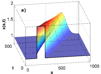
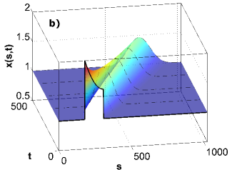
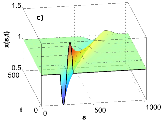
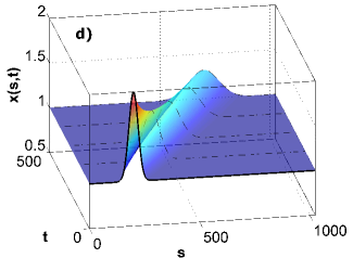
Figure 1: Initial conditions and their evolutions with the linear advection-diffusion equation: (a) flat top-hat (FTH), (b) quadratic top-hat (QTH), (c) window sinusoid (WS), and (d) squared-exponential (SE). The first two initial conditions (a, b) exhibit sparse representation in the wavelet domain while the next two (c, d) show nearly sparse representation in the discrete cosine domain (DCT). Initial conditions are evolved under the linear advection-diffusion equation (14) with $\epsilon=4\,[{\rm L}^{2}/{\rm T}]$ and $a=1\,[{\rm L}/{\rm T}]$. The broken lines show the time instants where the low-resolution and noisy observations are available in the assimilation interval.

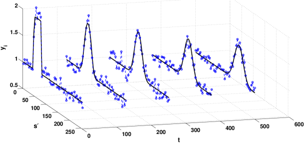
Figure 2: A sample representation of the available low-resolution (solid lines) and noisy observations (broken lines with circles) in every 125 [T] time steps in the assimilation window for the flat top-hat initial condition. Here, the observation error covariance is set to $\mathbf{R}=\sigma_{r}^{2}\mathbf{I}$ with $\sigma_{r}=0.08$ equivalent to ${\rm SNR}=20\,\log\left(\sigma_{\mathbf{x}_{0}}/\sigma_{r}\right)\approx 12$ dB.

4.2.3 Observation and Background Error

The observations and background errors are important components of a data assimilation system that determine the quality and information content of the analysis. Clearly, the nature and behavior of the errors are problem-dependent and need to be carefully investigated in a case by case study. It needs to be stressed that from a probabilistic point of view, the presented formulation for the $\ell_{1}$-norm RVDA assumes that both of the error components are unimodal and can be well explained by the class of Gaussian covariance models. Here, for observation error, we only consider a stationary white Gaussian measurement error, $\mathbf{v}\sim\mathcal{N}\left(0,\,\mathbf{R}\right)$, where $\mathbf{R}=\sigma_{r}^{2}\mathbf{I}$ (Figure 2).

However, as discussed in [Gaspari and Cohn, 1999], the background error can often exhibit a correlation structure. In this study the first and second order auto-regressive (AR) Gaussian Markov processes, are considered for mathematical simulation of a possible spatial correlation in the background error; see Gaspari and Cohn [1999] for a detailed discussion about the error covariance models for data assimilation studies.

The AR(1), also known as the Ornestein-Ulenbeck process in infinite dimension, has an exponential covariance function $\rho(\tau)\propto e^{-\alpha\left|\tau\right|}$. In this covariance function, $\tau$ denotes the lag either in space or time, and the parameter $\alpha$ determines the decay rate of the correlation. The inverse of the correlation decay rate $l_{c}=1/\alpha$ is often called the characteristic correlation length of the process. The covariance function of the AR(1) model has been studied very well in the context of stochastic process [e.g., Durrett, 1999] and estimation theory [e.g., Levy, 2008]. For example, it is shown by Levy [2008, p. 298] that the eigenvalues are monotonically decreasing which may give rise to a very ill-conditioned covariance matrix in the discrete space, especially for small $\alpha$ or large correlation length. The covariance function of the AR(2) is more complicated than the AR(1); however, it has been shown that in special cases, its covariance function can be explained by $\rho(\tau)\propto e^{-\alpha\left|\tau\right|}\left(1+\alpha\left|\tau\right|\right)$ [Gaspari and Cohn, 1999; Stein, 1999, p. 31]. Note that, both of these covariance models are stationary and also isotropic as they are only a function of the magnitude of the correlation lag [Rasmussen and Williams, 2006, pp. 82]. Consequently, the discrete background error covariance is a Hermitian Toeplitz matrix and can be decomposed into a scalar standard deviation and a correlation matrix as $\mathbf{B}=\sigma_{b}^{2}\mathbf{C}_{b}$, where

$$\mathbf{C}_{b}=\begin{bmatrix}\rho(0)&\rho(1)&\cdots&\rho(m)\\ \rho(1)&\rho(0)&\ddots&\vdots\\ \vdots&\ddots&\ddots&\rho(1)\\ \rho(m)&\cdots&\rho(1)&\rho(0)\end{bmatrix}\in\mathbb{R}^{m\times m}.$$

For the same values of $\alpha$, it is clear that the AR(2) correlation function decays slower than that of the AR(1). Figure 3 shows empirical estimation of the condition number of the reconstructed correlation matrices at different dimensions ranging from $m=$4 to 1024. As is evident, the error covariance of the AR(2) has a larger condition number than that of AR(1) for the same value of the parameter $\alpha$. Clearly, as the background error plays a very important role on the overall condition number of the Hessian in the cost function in (5), an ill-conditioned background error covariance makes the solution more unstable with larger uncertainty around the obtained analysis.

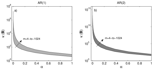
Figure 3: Empirical condition numbers of the background error covariance matrices as a function of parameter $\alpha$ and problem dimension ($m$) for the AR(1) in (a) and AR(2) in (b). The parameter $\alpha$ varies along the x-axis and $m$ varies along the different curves of the condition numbers with values between 4 and 1024. We recall that $\kappa\left(\mathbf{B}\right)$ is the ratio between the largest and smallest singular values of $\mathbf{B}$. In (a) the covariance matrix is $\mathbf{B}_{ij}=e^{-\alpha\left|i-j\right|}$ and in (b) $\mathbf{B}_{ij}=e^{-\alpha\left|i-j\right|}\left(1+\alpha\left|i-j\right|\right)$, $1\leq i,\,j\leq m$. It is seen that the condition numbers of the AR(2) model are significantly larger than those of the AR(1) model for the same values of the parameter $\alpha$.

Figure 4 shows a sample path of the chosen error models for the background error. Generally speaking, a correlated error contains large-scale (low-frequency) components that can corrupt the main spectral components of the true state at the same frequency range. Therefore, this type of error can superimpose with the large-scale characteristic features of the initial state and its removal is naturally more difficult than that of the white error via a data assimilation methodology.

Figure 4: Sample paths of the used correlated background error: (a) the sample path for the AR(1) covariance matrix with $\alpha^{-1}=150$, and (b) the sample path for the AR(2) covariance matrix with $\alpha^{-1}=25$. The paths are generated by multiplying a standard white Gaussian noise $\mathbf{e}\sim\mathcal{N}\left(0,\,\mathbf{I}\right)$ form the left by the lower triangular matrix $\mathbf{L}$, obtained by Cholesky factorization of the background error covariance matrix, that is $\mathbf{B}=\mathbf{LL}^{{\rm T}}$. It is seen that for small $\alpha$, the sample paths exhibit large scale oscillatory behavior that can potentially corrupt low-frequency components of the underlying state.

4.3 Results of Assimilation Experiments

In this subsection, we present the results of the proposed regularized data assimilation as expressed in equation (12). We first present the results for the white background error and then discuss the correlated error scenarios. As previously explained, the first two initial conditions exhibit sharp transitions and are naturally sparse in the wavelet domain. For those initial states (Figure 1a, b) we have used classic orthogonal wavelet transformation by Mallat [1989]. Indeed, the columns of $\mathbf{\Phi}\in\mathbb{R}^{1024\times 1024}$ in this case contain the chosen wavelet basis that allow us to decompose the initial state of interest into its wavelet representation coefficients, as $\mathbf{c}=\mathbf{\Phi}\mathbf{x}$ (forward wavelet transform). On the other hand, due to the orthogonality of the chosen wavelet $\mathbf{\Phi}\mathbf{\Phi}^{{\rm T}}=\mathbf{I}$, rows of $\mathbf{\Phi}^{{\rm T}}$ contain the wavelet basis that allows us to reconstruct the initial state from its wavelet representation coefficients, that is $\mathbf{x}=\mathbf{\Phi}^{{\rm T}}\mathbf{c}$ (inverse wavelet transform). We used a full level of decomposition without any truncation of wavelet decomposition levels to produce a fully sparse representation of the initial state. For example, in our case where $\mathbf{x}\in\mathbb{R}^{1024}$, we have used ten levels of decomposition.

For the last two initial states (Figure 1c, d) we used DCT transformation [e.g., Rao and Yip, 1990] which expresses the state of interest by a linear combination of the oscillatory cosine functions at different frequencies. It is well understood that this basis has a very strong compaction capacity to capture the energy content of sufficiently smooth states and sparsely represent them via a few elementary cosine waveforms. Note that, this transformation is also orthogonal ($\mathbf{\Phi}\mathbf{\Phi}^{{\rm T}}=\mathbf{I}$) and contrary to the Fourier transformation, the expansion coefficients are real.

4.3.1 White Background Error

For the white background and observation error covariance matrices ($\mathbf{B}=\sigma_{b}^{2}\mathbf{I}$, $\mathbf{R}=\sigma_{r}^{2}\mathbf{I}$ ), we considered $\sigma_{b}=0.10$ (${\rm SNR}\cong 10.5$ dB) and $\sigma_{r}=0.08$ (${\rm SNR}\cong 12$ dB), respectively. Some results are shown in Figure 5 for the selected initial conditions. It is clear that the $\ell_{1}$-norm regularized solution markedly outperforms the classic 4D-Var solutions in terms of the selected metrics. Indeed, in the regularized analysis the error is sufficiently suppressed and filtered, while characteristic features of the initial state are well-preserved. On the other hand, classic solutions typically over-fitted and followed the background state rather than extracting the true state. As a result, we can argue that for the white error covariance the classic 4D-Var has a very weak filtering effect which is an essential component of an ideal data assimilation scheme. This over-fitting may be due to the redundant (over-determined) formulation of the classic 4D-Var; see [Hawkins, 2004] for a general explanation on overfitting problems in statistical estimators and also see Daley [1993, p.41].

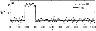
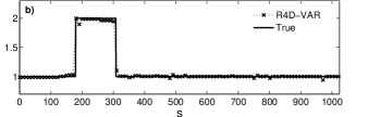
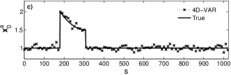
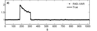
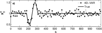
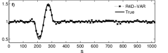
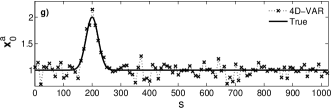
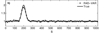
Figure 5: The results of the classic 4D-Var (left panel) versus the results of $\ell_{1}$-norm R4D-Var (right panel) for the tested initial conditions in a white Gaussian error environment. The solid lines are the true initial conditions and the crosses represent the recovered initial states or the analysis. In general, the results of the classic 4D-Var suffer from overfitting while the background and observation errors are suppressed and the sharp transitions and peaks are effectively recovered in the regularized analysis.

The average of the results for 30 independent runs is reported in Table 1. Three different lump quality metrics are examined as follows:

$${\rm MSE}_{r} = \left\|\mathbf{x}_{0}^{t}-\mathbf{x}_{0}^{a}\right\|_{2}/\left\|\mathbf{x}_{0}^{t}\right\|_{2}$$

$${\rm MAE}_{r} = \left\|\mathbf{x}_{0}^{t}-\mathbf{x}_{0}^{a}\right\|_{1}/\left\|\mathbf{x}_{0}^{t}\right\|_{1}$$

$${\rm BIAS}_{r} = \left|\mathbf{\bar{x}}_{0}^{t}-\mathbf{\bar{x}}_{0}^{a}\right|/\left|\mathbf{\bar{x}}_{0}^{t}\right|$$ (19)

namely, relative mean squared error $\left({\rm MSE}_{r}\right)$, relative mean absolute error $\left({\rm MAE}_{r}\right)$, and relative Bias $\left({\rm BIAS}_{r}\right)$. In (19) $\mathbf{x}_{0}^{t}$ denotes the true initial condition, $\mathbf{x}_{0}^{a}$ is the analysis, and upper bar denote the expected value. It is seen that based on the selected lump quality metrics, the $\ell_{1}$-norm R4D-Var significantly outperforms the classic 4D-Var. In general, the ${\rm MAE}_{r}$ metric is improved more than the ${\rm MSE}_{r}$ metric in the presented experiments. The best improvement is obtained for the flat top-hat initial condition (FTH), where the sparsity is very strong compared to the other initial conditions. In other words, the $\ell_{1}$-norm R4D-Var is more effective for stronger sparsity of the initial state. The ${\rm MSE}_{r}$ metric is improved almost three orders of magnitude, while the ${\rm MAE}_{r}$ improvement reaches up to six orders of magnitude in the FTH initial condition. We need to note that although the trigonometric functions can be sparsely represented in the DCT domain, here we used a window sinusoid, which suffers from discontinuities over the edges and can not be perfectly sparsified in the DCT domain. However, we see that even in a weaker sparsity, the results of the $\ell_{1}$-norm R4D-Var are still much better than the classic solution.

White Background Error
	${\rm MSE}_{r}$		${\rm MAE}_{r}$		${\rm BIAS}_{r}$
	R4D-Var	4D-Var	R4D-Var	4D-Var	R4D-Var	4D-Var
FTH	0.0188	0.0690	0.0099	0.0589	0.0016	0.0004
QTH	0.0152	0.0515	0.0083	0.0414	0.0030	0.0016
WS	0.0296	0.0959	0.0229	0.0771	0.0038	0.0022
SE	0.0316	0.0899	0.0235	0.0728	0.0018	4.26${\rm e}-5$

Table 1: Expected values of the ${\rm MSE}_{r}$, ${\rm MAE}_{r}$, and ${\rm BIAS}_{r}$, defined in (19), for 30 independent runs. The background and observation errors are white ($\mathbf{B}=\sigma_{b}^{2}\mathbf{I}$, $\mathbf{R}=\sigma_{r}^{2}\mathbf{I}$ ), where $\sigma_{b}=0.10$ (${\rm SNR}\cong 10.5$ dB) and $\sigma_{r}=0.08$ (${\rm SNR}\cong 12$ dB). The initial conditions are: flat top-hat (FTH), quadratic top-hat (QTH), window sinusoid (WS), and squared-exponential (SE). The results are reported for both the classic 4D-Var and the regularized 4D-Var (R4D-Var).

4.3.2 Correlated background error

In this part, the background error $\mathbf{B}=\sigma_{b}^{2}\mathbf{C}_{b}$ is considered to be correlated. As previously discussed, typically longer correlation length creates ill-conditioning in the background error covariance matrix and makes the problem more unstable. On the other hand, the correlated background error covariance imposes smoothness on the analysis [see, Gaspari and Cohn, 1999], improves filtering effects, and makes the classic solution to be less prone to overfitting. In this subsection, we examine the effect of correlation length on the solution of data assimilation and compare the results of the sparsity promoting R4D-Var with the classic 4D-Var. Here, we do not apply any preconditioning as the goal is to emphasize on the stabilizing role of the $\ell_{1}$-norm regularization in the presented formulaiton. In addition, for brevity, the results are only reported for the top-hat and window sinusoid initial condition, which are solved in the wavelet and DCT domains, respectively.

a)

Results for the AR(1) background error

As is evident, in this case, the background state is defined by adding AR(1) correlated error to the true state (6a,d) which is known to us for these experimental studies. Figure 6 demonstrates that in the case of correlated error the classic 4D-Var is less prone to overfitting compared to the case of the uncorrelated error in Figure 5. Typically in the flat top-hat initial condition (FTH) with sharp transitions, the classic solution fails to capture those sharp jumps and becomes spoiled around those discontnuities (Figure 6b). For the trigonometric initial condition (WS), the classic solution is typically overly smooth and can not capture the peaks (Figure 6e). These deficiencies in classic solutions typically become more pronounced for larger correlation lengths and thus more ill-conditioned problems. On the other hand, the $\ell_{1}$-norm R4D-Var markedly outperforms the classic method by improving the recovery of the sharp transitions in FTH and peaks in WS (Figure 6).

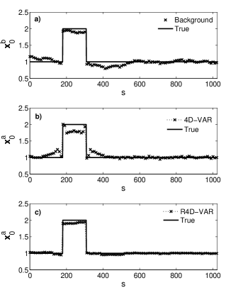
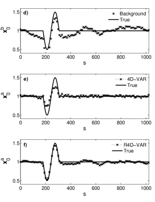
Figure 6: Comparison of the results of the classic 4D-Var (b, e) and $\ell_{1}$-norm R4D-Var (c, f) for the top-hat (left panel) and window sinusoid (right panel) initial conditions. The background states in (a) and (d) are defined by adding correlated errors using an AR(1) covariance model of $\rho(\tau)\propto e^{-\alpha\left|\tau\right|}$, where $\alpha=1/250$. The results show that the $\ell_{1}$-norm R4D-Var improves recovery of sharp jumps and peaks and results in a more stable solution compared to the classic 4D-Var; see Figure 7 for quantitative results.

We examined a relatively wide range of applicable correlation lengths, $\alpha^{-1}\in\left\{1,\,10,\,25,\,50,\,250,\,1000\right\}$, which correspond to decades of variations ranging from $10^{1}$ to $10^{6}$ in the condition number $\kappa\left(\mathbf{B}\right)$ of the background error covariance matrices (see Figure 3a). The assimilation results using different correlation lengths are demonstrated in Figure 7. To have a robust conclusion about comparison of the proposed R4D-Var with the classic 4D-Var, the plots in this figure demonstrate the expected values of the quality metrics for 30 independent runs.

It can be seen that for small error correlation lengths ($\alpha^{-1}\lesssim 25$), the improvement of the R4D-Var is very significant while in the medium range ($25\lesssim\alpha^{-1}\lesssim 50$) the classic solution becomes more competitive and closer to the regularized analysis. As previously mentioned, this improvement in the classic solutions is mainly due to the smoothing effect of the background covariance matrix. However, for larger correlation lengths ($\alpha^{-1}\gtrsim 50$), the differences of the two methods are more drastic as the classic solutions become more unstable and fail to capture the underlying structure of the initial state of interest. In general, we see that the ${\rm MSE}_{r}$ and ${\rm MAE}_{r}$ metrics are improved for all examined background error correlation lengths. As expected, the regularized solutions are slightly biased compared to classic solutions; however, the magnitude of the bias is not significant compared to the mean value of the initial state (see Figure 7). Figure 7 also shows a very important outcome of regularization which implies that the R4D-Var is almost insensitive to the studied range of correlation length and thus condition number of the problem. This confirms the stabilizing role of regularization and needs to be further studied for large scale and operational data assimilation problems. Another important observation is that, for extremely correlated background error, the classic R4D-Var may produce analysis with larger bias than the proposed R4D-Var (Figure 7c). This unexpected result might be due to the presence of spurious bias in the background state coming from a strongly correlated error. In other words, a strongly correlated error may shift the mean value of the background state significantly and create a large bias in the solution of the classic 4D-Var. In this case, the improved performance of the R4D-Var may be due to its stronger stability and filtering properties.

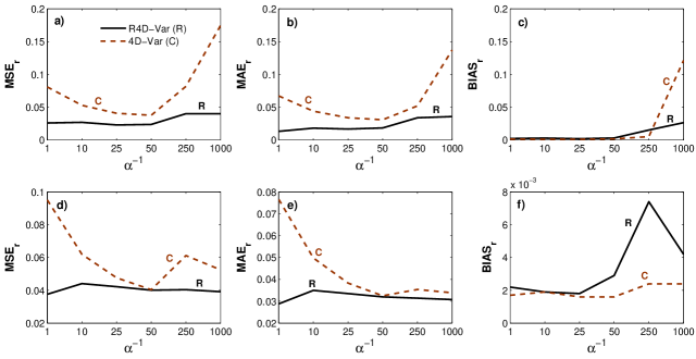
Figure 7: Comparison of the results of the proposed $\ell_{1}$-norm R4D-Var (solid lines) and the classic 4D-Var (broken lines) under the AR(1) background error for different correlation characteristic length scales ($\alpha^{-1}$). Top panel: (a-c) the chosen quality metrics for the top-hat initial condition (FTH); Bottom panel: (d-f) the metrics for the window sinusoid initial condition (WS). These results, averaged over 30 independent runs, demonstrate significant improvements in recovering the analysis state by the proposed $\ell_{1}$-norm R4D-Var compared to the classic 4D-Var.

b)

Results for the AR(2) background error

The AR(2) model is suitable for errors with higher order Markovian structure compared to the AR(1) model. As is seen in Figure (4), the condition number of the AR(2) covariance matrix is much larger than the AR(1) for the same values of the parameter $\alpha$ in the studied covariance models. Here, we limited our experiments to fewer characteristic correlation lengths of $\alpha^{-1}=\left\{1,\,5,\,25,\,50\right\}$. We constrained our considerations to $\alpha^{-1}\lesssim 50$ , because for larger values (slower correlation decay rates) the condition number of $\mathbf{B}$ exceeds $10^{8}$ and almost both methods failed to obtain the analysis without any preconditioning effort.

In our case study, for $\alpha^{-1}\lesssim 25$, where $\kappa(\mathbf{B})\lesssim 10^{6}$, the proposed R4D-Var outperforms the 4D-Var similar to what has been explained for the AR(1) error in the previous subsection. However, we found that for $25\lesssim\alpha^{-1}\lesssim 50$, where $10^{6}\lesssim\kappa(\mathbf{B})\lesssim 10^{8}$, without proper preconditioning, the used conjugate gradient algorithm fails to obtain the analysis state in the 4D-Var (Table 2). On the other hand, due to the role of the proposed regularization, the R4D-Var remains sufficiently stable; however, its effectiveness deteriorated compared to the cases where the condition numbers were lower. This observation verifies the known role of the proposed regularization for improving the condition number of the variational data assimilation problem.

AR(2) – Background Error
	$\alpha^{-1}$	${\rm MSE}_{r}$		${\rm MAE}_{r}$		${\rm BIAS}_{r}$
		R4D-Var	4D-Var	R4D-Var	4D-Var	R4D-Var	4D-Var
FTH	1	0.0254	0.0754	0.0162	0.0629	0.0023	0.0016
	5	0.0328	0.0643	0.0212	0.0534	0.0043	0.0018
	25	0.0722	-	0.0608	-	0.0187	-
	50	0.0742	-	0.0582	-	0.0268	-
WS	1	0.0363	0.0887	0.0272	0.0715	0.0029	0.0012
	5	0.0708	0.0906	0.0571	0.0529	0.0106	0.0017
	25	0.0877	-	0.0710	-	0.0243	-
	50	0.0898	-	0.0747	-	0.0361	-

Table 2: Expected values of the ${\rm MSE}_{r}$, ${\rm MAE}_{r}$, and ${\rm BIAS}_{r}$ defined in (19), for 30 independent runs. The background and observation errors are modeled by the first order auto-regressive ($\mathbf{B}=\sigma_{b}^{2}\mathbf{C}_{B}$) and white ($\mathbf{R}=\sigma_{r}^{2}\mathbf{I}$ ) Gaussian processes, where $\sigma_{b}=0.10$ (${\rm SNR}\cong 10.5$ dB) and $\sigma_{r}=0.08$ (${\rm SNR}\cong 12$ dB). The parameter $\alpha$ denotes the correlation decay rate in the AR(2) covariance function $\rho(\tau)\propto e^{-\alpha\left|\tau\right|}\left(1+\alpha\left|\tau\right|\right)$. The studied initial conditions are: flat top-hat (FTH), and window sinusoid (WS) and the results are reported for both the classic 4D-Var and the regularized 4D-Var (R4D-Var). The dash lines in the table denote that the classic method failed to return a solution without any pre-conditioning.

4.3.3 Selection of the regularization parameters

As previously explained, the regularization parameter $\lambda$ plays a very important role in making the analysis sufficiently faithful to the observations and background state, while preserving the underlying regularity of the analysis. To the best of our knowledge, no general methodology exists which will produce an exact and closed form solution for the selection of this parameter, especially for the proposed $\ell_{1}$-norm regularization [see, Hansen, 2010, chap.5]. Here, we chose the regularization parameter $\lambda$ by trial and error based on a minimum mean squared error criterion (Figure 8). As a rule of thumb, we found that in general $\lambda\lesssim 0.05\left\|\mathbf{b}\right\|_{\infty}$ yields reasonable results. We also realized that under similar error signal-to-noise ratio, the selection of $\lambda$ depends on some important factors such as, the pre-selected basis, the degree of ill-conditioning of the problem, and more importantly the ratio between the dominant frequency components of the state and the error.

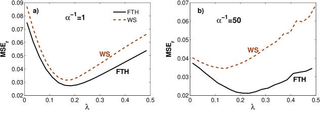
Figure 8: The relative mean squared error versus the regularization parameter obtained for the AR(1) background error for different characteristic correlation length (a) $\alpha^{-1}=1$, and (b) $\alpha^{-1}=50$. FTH and WS denote the flat top-hat and window sinusoid initial conditions, respectively.

5 Summary and Discussion

We have discussed the concept of sparse regularization in variational data assimilation and examined a simple but important application of the proposed problem formulation to the advection-diffusion equation, relevant to land surface heat and mass flux studies. In particular, we extended the classic formulations by leveraging sparsity for solving data assimilation problems in wavelet and spectral domains. The basic claim is that if the underlying state of interest exhibits sparsity in a pre-selected basis, this prior information can serve to further constrain and improve the quality of the analysis cycle and thus the forecast skill. We demonstrated that the regularized variational data assimilation (RVDA) not only shows better interpolation properties but also exhibits improved filtering attributes by effectively removing small scale noisy features that possibly do not satisfy the underlying governing physical laws. Furthermore, it is argued that the $\ell_{1}$-norm RVDA is more robust to the possible ill-conditioning of the data assimilation problem and leads to more stable analysis compared to the classic methods.

We explained that, from the statistical point of view, this prior knowledge speaks for the spatial intrinsic non-Gaussian structure of the state variable of interest which can be well parameterized and modeled in a properly chosen basis. We discussed that selection of the sparsifying basis can be seen as a statistical model selection problem which can be guided by studying the distribution of the representation coefficients.

Further research needs to be devoted to developing methodologies to: (a) characterize the analysis covariance, especially using ensemble based approaches; (b) automatize the selection of the regularization parameter and study its impact on various applications of data assimilation problems; (c) apply the methodology in an incremental setting to tackle non-linear observation operators [Courtier et al., 1994]; and (d) study the role of preconditioning on the background error covariance for very ill-conditioned data assimilation problems in regularized variational data assimilation settings.

Furthermore, a promising area of future research is that of developing and testing $\ell_{1}$-norm RVDA to tackle non-linear measurement and model equations in a hybrid variational-ensemble data setting. Basically, a crude framework can be cast as follows: (1) given the analysis and its covariance at previous time step, properly generate an ensemble of analysis state; (2) use the analysis ensembles to generate forecasts or background ensembles via the model equation and then compute the background ensemble mean and covariance; (3) given the background ensembles, obtain observation ensembles via the observation equation and then obtain the ensemble observation covariance; (4) solve an $\ell_{1}$-norm RVDA problem similar to that of (12) for each ensemble to obtain ensemble analysis states at present time; (5) compute the ensemble analysis mean and covariance and use them to forecast the next time step; and (6) repeat the recursion.

Appendix A Appendix

A.1 Quadratic Programming form of the $\ell_{1}$-norm RVDA

To obtain the quadratic programming (QP) form presented in (13), we follow the general strategy proposed in the seminal work by Chen et al. [2001]. To this end, let us expand the $\ell_{1}$-norm regularized variational data assimilation ($\ell_{1}$-RVDA) problem in (12) as follows:

$$\underset{\mathbf{x}_{0}}{{\rm minimize}}\,\,\,\left\{\frac{1}{2}\mathbf{x}_{0}^{{\rm T}}\left(\mathbf{B}^{-1}+\underline{\mathbf{H}}{}^{{\rm T}}\mathbf{R}^{-1}\mathbf{\underline{\mathbf{H}}}\right)\mathbf{x}_{0}-\left(\mathbf{B}^{-1}\mathbf{x}_{0}^{b}+\mathbf{\underline{\mathbf{H}}}^{{\rm T}}\mathbf{R}^{-1}\underline{\mathbf{y}}\right)^{{\rm T}}\mathbf{x}_{0}+\lambda\left\|\mathbf{\Phi}\mathbf{x}_{0}\right\|_{1}\right\}.$$ (A.1)

Assuming $\mathbf{c}_{0}=\mathbf{\Phi}\mathbf{x}_{0}\in\mathbb{R}^{m}$, then the above problem can be rewritten as,

$$\underset{\mathbf{z}_{0}}{{\rm minimize}}\,\,\,\left\{\frac{1}{2}\mathbf{c}_{0}^{{\rm T}}\mathbf{Q}\mathbf{c}_{0}+\mathbf{b}^{{\rm T}}\mathbf{c}_{0}+\lambda\left\|\mathbf{c}_{0}\right\|_{1}\right\},$$ (A.2)

where, $\mathbf{Q}=\mathbf{\Phi}^{-{\rm T}}\left(\mathbf{B}^{-1}+\mathbf{\underline{\mathbf{H}}}^{{\rm T}}\mathbf{R}^{-1}\underline{\mathbf{H}}\right)\mathbf{\Phi}^{-1}$ and $\mathbf{b}=-\mathbf{\Phi}^{-{\rm T}}\left(\mathbf{B}^{-1}\mathbf{x}_{0}^{b}+\underline{\mathbf{H}}^{{\rm T}}\mathbf{R}^{-1}\underline{\mathbf{y}}\right)$. Having $\mathbf{c}_{0}=\mathbf{u}_{0}-\mathbf{v}_{0}$, where $\mathbf{u}_{0}=\max\left(\mathbf{c}_{0},\,0\right)\in\mathbb{R}^{m}$ and $\mathbf{v}_{0}=\max\left(-\mathbf{c}_{0},\,0\right)\in\mathbb{R}^{m}$ encode the positive and negative components of $\mathbf{c}_{0}$, problem (A.2) can be represented as follows:

$$\underset{\mathbf{x}_{0}}{{\rm minimize}\,\,\,} \left\{\frac{1}{2}\left(\mathbf{u}_{0}-\mathbf{v}_{0}\right)^{{\rm T}}\mathbf{Q}\left(\mathbf{u}_{0}-\mathbf{v}_{0}\right)+\mathbf{b}^{{\rm T}}\left(\mathbf{u}_{0}-\mathbf{v}_{0}\right)+\lambda 1_{m}^{{\rm T}}\left(\mathbf{u}_{0}+\mathbf{v}_{0}\right)\right\}$$

$$\,\,\,\,\,\,\,\,\,\,{\rm subject}\,{\rm to\,\,\,\,\,\,}\mathbf{u}_{0}\succcurlyeq 0,\,\mathbf{v}_{0}\succcurlyeq 0$$ (A.3)

Stacking $\mathbf{u}_{0}$ and $\mathbf{v}_{0}$ in $\mathbf{w}_{0}=[\mathbf{u}_{0}^{{\rm T}},\,\mathbf{v}_{0}^{{\rm T}}]^{{\rm T}}$, the more standard QP formulation of the problem is immediately followed as:

$$\underset{\mathbf{w}_{0}}{{\rm minimize}}\,\,\, \left\{\frac{1}{2}\mathbf{w}_{0}^{{\rm T}}\begin{bmatrix}\begin{array}[]{rr}\mathbf{Q}&-\mathbf{Q}\\ -\mathbf{Q}&\mathbf{Q}\end{array}\end{bmatrix}\mathbf{w}_{0}+\left(\lambda\mathbf{1}_{2m}+\begin{bmatrix}\begin{array}[]{r}\mathbf{b}\\ -\mathbf{b}\end{array}\end{bmatrix}\right)^{{\rm T}}\mathbf{w}_{0}\right\}$$

$$\,\,\,\,\,\,\,\,\,\,{\rm subject}\,{\rm to\,\,\,\,\,\,}\mathbf{w}_{0}\succcurlyeq 0.$$ (A.4)

Obtaining $\mathbf{\hat{w}}_{0}=[\mathbf{\hat{u}}_{0}^{{\rm T}},\,\mathbf{\hat{v}}_{0}^{{\rm T}}]^{{\rm T}}\in\mathbb{R}^{2m}$ as the solution of (A.4), one can easily recover $\mathbf{\hat{c}}_{0}=\hat{\mathbf{u}}_{0}-\hat{\mathbf{v}}_{0}$ and thus the initial state of interest $\mathbf{\hat{x}}_{0}=\mathbf{\Phi}^{-1}\hat{\mathbf{c}}_{0}$.

The dimension of the QP representation (A.4) is twice that of the original $\ell_{1}$-RVDA problem (A.1). However, using iterative first order gradient based methods, which are often the only practical option for large-scale data assimilation problems, it is easy to show that the effect of this dimensionality enlargement is minor on the overall cost of the problem. Because, one can easily see that obtaining the gradient of the cost function in (A.4) only requires to compute

$$\begin{bmatrix}\begin{array}[]{rr}\mathbf{Q}&-\mathbf{Q}\\ -\mathbf{Q}&\mathbf{Q}\end{array}\end{bmatrix}\mathbf{w}_{0}=\begin{bmatrix}\begin{array}[]{r}\mathbf{Q}\left(\mathbf{u}_{0}-\mathbf{v}_{0}\right)\\ -\mathbf{Q}\left(\mathbf{u}_{0}-\mathbf{v}_{0}\right)\end{array}\end{bmatrix},$$

which mainly requires matrix-vector multiplication in $\mathbb{R}^{m}$ [see; e.g., Figueiredo et al., 2007].

A.2 Upper Bound of the Regularization Parameter

Here to derive the upper bound for the regularization parameter in the $\ell_{1}$-RVDA problem, we follow a similar approach as suggested for example by Kim et al. [2007]. Let us refer back to the problem (A.2) which is convex but not differentiable at the origin. Obviously, $\mathbf{c}_{0}^{a}$ is a minimizer if and only if the cost function $\mathcal{J}_{R4D}(\mathbf{c}_{0})$ in (A.2) is sub-differentiable at $\mathbf{c}_{0}^{a}$ and thus

$$0\in\partial\mathcal{J}_{R4D}(\mathbf{c}_{0}^{a}),$$

where, $\partial\mathcal{J}_{R4D}(\mathbf{c}_{0}^{a})$ denotes the sub-differential set at the solution point or analysis coefficients in the selected basis. Given that

$$\partial\mathcal{J}_{R4D}(\mathbf{c}_{0}^{a})=\mathbf{Q}\mathbf{c}_{0}^{a}+\mathbf{b}+\lambda\partial\left(\left\|\mathbf{c}_{0}^{a}\right\|_{1}\right),$$

we have

$$-\mathbf{Q}\mathbf{c}_{0}^{a}-\mathbf{b}\in\lambda\partial\left(\left\|\mathbf{c}_{0}^{a}\right\|_{1}\right).$$

and thus for $\mathbf{c}_{0}^{a}=\mathbf{0}_{m}$, $\mathbf{0}_{m}=\left[0,\,\ldots,\,0\right]^{{\rm T}}\in\mathbb{R}^{m}$, one can obtain the following vector inequality

$$-\lambda\mathbf{1}_{m}\preceq-\mathbf{b}\preceq\lambda\mathbf{1}_{m},$$

which implies that $\left\|\mathbf{b}\right\|_{\infty}\leq\lambda$. Therefore $\lambda$ must be less than $\left\|\mathbf{b}\right\|_{\infty}$ to obtain nonzero analysis coefficients in problem (A.2) and thus (A.1).

A.3 Gradient Projection Method

Gradient projection (GP) method is an efficient and convergent optimization method to solve convex optimization problems over convex sets [see, Bertsekas, 1999, pp. 228]. This method is of particular interest, especially, when the constraints form a convex set $\mathcal{C}$ with simple projection operator. The cost function $\mathcal{J}_{R4D}(\mathbf{w}_{0})$ in (13) is a quadratic function that need to be minimized on non-negative orthant $\mathcal{C}=\{\mathbf{w}_{0}|\,\,w_{0,i}\geq 0\,\,\forall\,i=1,\ldots,2m\}$ as follows:

$$\hat{\mathbf{w}}_{0} = {\rm argmin}\,\left\{\mathcal{J}_{R4D}(\mathbf{w}_{0})\right\}$$ (A.5)

$$\,\,{\rm s.t.\,\,\mathbf{w}_{0}\succeq 0}.$$

For this particular problem, the GP method amounts obtaining the following fixed point:

$$\mathbf{w}_{0}^{*}=\left[\mathbf{w}_{0}^{*}-\beta\nabla\mathcal{J}_{R4D}(\mathbf{w}_{0}^{*})\right]^{+},$$ (A.6)

where $\beta$ is a stepsize along the descent direction and for every element of $\mathbf{w}_{0}$

$$\left[w_{0}\right]^{+}=\begin{cases}0&\,\,{\rm if}\,\,w_{0}\leq 0\\ w_{0}&{\rm otherwise,}\end{cases}$$ (A.7)

denotes the Euclidean projection operator onto the non-negative orthant. As is evident, the fixed point can be obtained iteratively as

$$\mathbf{w}_{0}^{k+1}=\left[\mathbf{w}_{0}^{k}-\beta^{k}\nabla\mathcal{J}_{R4D}(\mathbf{w}_{0}^{k})\right]^{+}.$$ (A.8)

Thus, if the descent at step $k$ is feasible, that is $\mathbf{w}_{0}^{k}-\beta^{k}\nabla\mathcal{J}_{R4D}(\mathbf{w}_{0}^{k})\succeq 0$, the GP iteration becomes an ordinary unconstrained steepest descent method, otherwise the result is mapped back onto the feasible set by the projection operator in (A.7). In effect, the GP method finds iteratively the closest feasible point in the constraint set to the solution of the original unconstrained minimization.

In our study, the stepsize $\beta^{k}$ was selected using the Armijo rule, or the so-called backtracking line search, that is a convergent and very effective stepsize rule. This stepsize rule depends on two constants $0<\xi<0.5$ , $0<\varsigma<1$ and assumed to be $\beta^{k}=\varsigma^{m_{k}}$, where $m_{k}$ is the smallest non-negative integer for which

$$\mathcal{J}_{R4D}\left(\mathbf{w}_{0}^{k}-\beta^{k}\nabla\mathcal{J}_{R4D}(\mathbf{w}_{0}^{k})\right)\leq\mathcal{J}_{R4D}(\mathbf{w}_{0}^{k})-\xi\beta^{k}\nabla\mathcal{J}_{R4D}(\mathbf{w}_{0}^{k})^{{\rm T}}\nabla\mathcal{J}_{R4D}(\mathbf{w}_{0}^{k}).$$ (A.9)

In our experiments the backtracking parameters are set to $\xi=0.2$ and $\varsigma=0.5$ [see, Boyd and Vandenberghe, 2004, pp.464 for more explanation]. In our coding, the iterations terminate if $\frac{\left\|\mathbf{w}_{0}^{k}-\mathbf{w}_{0}^{k-1}\right\|_{2}}{\left\|\mathbf{w}_{0}^{k-1}\right\|_{2}}\leq 10^{-5}$ or the number of iterations exceeds 100.

References

- Afshar and Marino [1978] Afshar, A., and M. A. Marino (1978), Model for simulating soil-water content considering evapotranspiration, Journal of Hydrology, 37(3–4), 309 – 322, 10.1016/0022-1694(78)90022-7.
- Anderson [2001] Anderson, J. L. (2001), An Ensemble Adjustment Kalman Filter for Data Assimilation, Mon. Wea. Rev., 129(12), 2884–2903, 10.1175/1520-0493(2001)129<2884:AEAKFF>2.0.CO;2.
- Bai et al. [1987] Bai, Z., J. Demmel, J. Dongarra, A. Ruhe, and H. Van Der Vorst (1987), Templates for the solution of algebraic eigenvalue problems: a practical guide, vol. 11, SIAM, Philadelphia.
- Barnard et al. [2000] Barnard, J., R. McCulloch, and X. Meng (2000), Modeling covariance matrices in terms of standard deviations and correlations, with application to shrinkage, Stat. Sinica, 10(4), 1281–1312.
- Bennett and McIntosh [1982] Bennett, A. F., and P. C. McIntosh (1982), Open Ocean Modeling as an Inverse Problem: Tidal Theory, J. Phys. Oceanogr., 12(10), 1004–1018, 10.1175/1520-0485(1982)012<1004:OOMAAI>2.0.CO;2.
- Bertsekas [1976] Bertsekas, D. (1976), On the Goldstein-Levitin-Polyak gradient projection method, IEEE Trans. Automat. Contr., 21(2), 174 – 184, 10.1109/TAC.1976.1101194.
- Bertsekas [1999] Bertsekas, D. P. (1999), Nonlinear Programming, 2nd ed., 794 pp., Athena Scientific, Belmont, MA.
- Boyd and Vandenberghe [2004] Boyd, S., and L. Vandenberghe (2004), Convex optimization, 716 pp., Cambridge University Press, New York.
- Budd et al. [2011] Budd, C., M. Freitag, and N. Nichols (2011), Regularization techniques for ill-posed inverse problems in data assimilation, Computers & Fluids, 46(1), 168–173, 10.1016/j.compfluid.2010.10.002.
- Candes and Tao [2006] Candes, E., and T. Tao (2006), Near-Optimal Signal Recovery From Random Projections: Universal Encoding Strategies?, IEEE Trans. Inform. Theory., 52(12), 5406–5425, 10.1109/TIT.2006.885507.
- Chan and Jin [2007] Chan, R. H.-F., and X.-Q. Jin (2007), An Introduction to Iterative Toeplitz Solvers, SIAM, Philadelphia.
- Chapra [2008] Chapra, S. C. (2008), Surface Water Quality Modeling, Waveland Press, Inc. IL, USA.
- Chen et al. [2001] Chen, S., D. Donoho, and M. Saunders (2001), Atomic Decomposition by Basis Pursuit, SIAM rev., 43(1), 129–159.
- Chen et al. [1998] Chen, S. S., D. L. Donoho, and M. A. Saunders (1998), Atomic decomposition by basis pursuit, SIAM J. Sci. Comput., 20, 33–61.
- Courtier and Talagrand [1990] Courtier, P., and O. Talagrand (1990), Variational assimilation of meteorological observations with the direct and adjoint shallow-water equations, Tellus A, 42(5), 531–549.
- Courtier et al. [1994] Courtier, P., J.-N. Thépaut, and A. Hollingsworth (1994), A strategy for operational implementation of 4D-VAR, using an incremental approach, Quart. J. Roy. Meteor. Soc., 120(519), 1367–1387, 10.1002/qj.49712051912.
- Daley [1993] Daley, R. (1993), Atmospheric data analysis, 472 pp., Cambridge University Press.
- Durrett [1999] Durrett, R. (1999), Essentials of Stochastic Processes, Springer-Verlag, N.Y.
- Ebtehaj and Foufoula-Georgiou [2013] Ebtehaj, A. M., and E. Foufoula-Georgiou (2013), On Variational Downscaling, Fusion and Assimilation of Hydro-meteorological States: A Unified Framework via Regularization, Water Resour. Res, under review.
- Elad [2010] Elad, M. (2010), Sparse and Redundant Representations: From Theory to Applications in Signal and Image Processing, 376 pp., Springer Verlag.
- Evensen [1994a] Evensen, G. (1994a), Sequential data assimilation with a nonlinear quasi-geostrophic model using Monte Carlo methods to forecast error statistics, J. Geophys. Res., 99(C5), 10,143–10,162.
- Evensen [1994b] Evensen, G. (1994b), Inverse methods and data assimilation in nonlinear ocean models, Physica D: Nonlinear Phenomena, 77(1–3), 108 – 129, 10.1016/0167-2789(94)90130-9, <ce:title>Special Issue Originating from the 13th Annual International Conference of the Center for Nonlinear Studies Los Alamos, NM, USA, 17&ndash;21 May 1993 </ce:title>.
- Fetter [1994] Fetter, C. (1994), Applied Hydrogeology, Prentice Hall, New Jersey, USA, Fourth Edition.
- Figueiredo et al. [2007] Figueiredo, M., R. Nowak, and S. Wright (2007), Gradient Projection for Sparse Reconstruction: Application to Compressed Sensing and Other Inverse Problems, IEEE J. Sel. Topics Signal Process., 1(4), 586–597, 10.1109/JSTSP.2007.910281.
- Freitag et al. [2010] Freitag, M. A., N. K. Nichols, and C. J. Budd (2010), L1-regularisation for ill-posed problems in variational data assimilation, PAMM, 10(1), 665–668, 10.1002/pamm.201010324.
- Freitag et al. [2012] Freitag, M. A., N. K. Nichols, and C. J. Budd (2012), Resolution of sharp fronts in the presence of model error in variational data assimilation, Quart. J. Roy. Meteor. Soc., 10.1002/qj.2002.
- Gaspari and Cohn [1999] Gaspari, G., and S. E. Cohn (1999), Construction of correlation functions in two and three dimensions, Quart. J. Roy. Meteor. Soc., 125(554), 723–757, 10.1002/qj.49712555417.
- Ghil [1989] Ghil, M. (1989), Meteorological data assimilation for oceanographers. Part I: Description and theoretical framework, Dyn. Atmos. Oceans, 13(3), 171–218.
- Ghil and Malanotte-Rizzoli [1991] Ghil, M., and P. Malanotte-Rizzoli (1991), Data Assimilation in Meteorology and Oceanography, pp. 141 – 266, Elsevier, 10.1016/S0065-2687(08)60442-2.
- Ghil et al. [1981] Ghil, M., S. Cohn, J. Tavantzis, K. Bube, and E. Isaacson (1981), Applications of Estimation Theory to Numerical Weather Prediction, in Dynamic Meteorology: Data Assimilation Methods, Applied Mathematical Sciences, vol. 36, edited by L. Bengtsson, M. Ghil, and E. Källén, pp. 139–224, Springer New York, 10.1007/978-1-4612-5970-1_5.
- Golub et al. [1999] Golub, G., P. Hansen, and D. O’Leary (1999), Tikhonov regularization and total least squares, SIAM J. Matrix Anal. Appl., 21(1), 185–194.
- Hansen [1998] Hansen, P. (1998), Rank-deficient and discrete ill-posed problems: numerical aspects of linear inversion, vol. 4, Society for Industrial Mathematics (SIAM), Philadelphia.
- Hansen [2010] Hansen, P. (2010), Discrete inverse problems: insight and algorithms, vol. 7, Society for Industrial & Applied Mathematics (SIAM), Philadelphia, PA, USA.
- Hansen and O’Leary [1993] Hansen, P., and D. O’Leary (1993), The use of the L-curve in the regularization of discrete ill-posed problems, SIAM J Sci Comput, 14(6), 1487–1503.
- Hansen et al. [2006] Hansen, P., J. Nagy, and D. Óleary (2006), Deblurring images: matrices, spectra, and filtering, vol. 3, Society for Industrial & Applied Mathematics (SIAM), Philadelphia, PA, USA.
- Hawkins [2004] Hawkins, D. M. (2004), The problem of overfitting, J. Chem. Inf. Comput. Sci., 44(1), 1–12.
- Hu and Islam [1995] Hu, Z., and S. Islam (1995), Prediction of Ground Surface Temperature and Soil Moisture Content by the Force-Restore Method, Water Resources Research, 31(10), 2531–2539, 10.1029/95WR01650.
- Ide et al. [1997] Ide, K., P. Courtier, M. Gill, and A. Lorenc (1997), Unified notation for data assimilation: Operational, sequential, and variational, J. Meteo. Soc. Japan, 75, 181–189.
- Jochum and Murtugudde [2006] Jochum, M., and R. Murtugudde (2006), Temperature advection by tropical instability waves, J. Phys. Oceanogr., 36(4), 592–605.
- Johnson et al. [2005a] Johnson, C., B. J. Hoskins, and N. K. Nichols (2005a), A singular vector perspective of 4D-Var: Filtering and interpolation, Quart. J. Roy. Meteor. Soc., 131(605), 1–19, 10.1256/qj.03.231.
- Johnson et al. [2005b] Johnson, C., N. K. Nichols, and B. J. Hoskins (2005b), Very large inverse problems in atmosphere and ocean modelling, Int. J. Numer. Meth. Fl., 47(8-9), 759–771, 10.1002/fld.869.
- Kalnay [2003] Kalnay, E. (2003), Atmospheric modeling, data assimilation, and predictability, 341 pp., Cambridge University Press, New York.
- Kim et al. [2007] Kim, S.-J., K. Koh, M. Lustig, S. Boyd, and D. Gorinevsky (2007), An Interior-Point Method for Large-Scale l1-Regularized Least Squares, IEEE J. Sel. Topics Signal Process., 1(4), 606–617, 10.1109/JSTSP.2007.910971.
- Kleist et al. [2009] Kleist, D. T., D. F. Parrish, J. C. Derber, R. Treadon, W.-S. Wu, and S. Lord (2009), Introduction of the GSI into the NCEP Global Data Assimilation System, Wea. Forecasting, 24(6), 1691–1705, 10.1175/2009WAF2222201.1.
- Lanser and Verwer [1999] Lanser, D., and J. Verwer (1999), Analysis of operator splitting for advection–diffusion–reaction problems from air pollution modelling, Journal of Computational and Applied Mathematics, 111(1–2), 201 – 216, 10.1016/S0377-0427(99)00143-0.
- Levy [2008] Levy, B. C. (2008), Principles of Signal Detection and Parameter Estimation, 1 ed., 639 pp., Springer Publishing Company, New York, USA, 10.1007/978-0-387-76544-0.
- Lewicki and Sejnowski [2000] Lewicki, M., and T. Sejnowski (2000), Learning overcomplete representations, Neural Comput., 12(2), 337–365.
- Liang et al. [1999] Liang, X., E. F. Wood, and D. P. Lettenmaier (1999), Modeling ground heat flux in land surface parameterization schemes, J. Geophys. Res., 104(D8), 9581–9600.
- Lin et al. [1998] Lin, Y.-L., R. L. Deal, and M. S. Kulie (1998), Mechanisms of cell regeneration, development, and propagation within a two-dimensional multicell storm, J. Atmos. Sci., 55(10), 1867–1886.
- Lorenc [1988] Lorenc, A. (1988), Optimal nonlinear objective analysis, Quart. J. Roy. Meteor. Soc., 114(479), 205–240.
- Lorenc [1986] Lorenc, A. C. (1986), Analysis methods for numerical weather prediction, Quart. J. Roy. Meteor. Soc., 112(474), 1177–1194, 10.1002/qj.49711247414.
- Lorenc et al. [2000] Lorenc, A. C., S. P. Ballard, R. S. Bell, N. B. Ingleby, P. L. F. Andrews, D. M. Barker, J. R. Bray, A. M. Clayton, T. Dalby, D. Li, T. J. Payne, and F. W. Saunders (2000), The Met. Office global three-dimensional variational data assimilation scheme, Quart. J. Roy. Meteor. Soc., 126(570), 2991–3012, 10.1002/qj.49712657002.
- Mallat [1989] Mallat, S. (1989), A theory for multiresolution signal decomposition: the wavelet representation, IEEE Trans. Pattern Anal. Mach. Intell., 11(7), 674–693, 10.1109/34.192463.
- Mallat [2009] Mallat, S. (2009), A wavelet tour of signal processing: the sparse way, 3rd ed., 805 pp., Elsevier /Academic Press.
- Moradkhani et al. [2005] Moradkhani, H., K.-L. Hsu, H. Gupta, and S. Sorooshian (2005), Uncertainty assessment of hydrologic model states and parameters: Sequential data assimilation using the particle filter, Water Resour. Res., 41(5), W05,012–.
- Nadarajah [2005] Nadarajah, S. (2005), A generalized normal distribution, J. Appl. Stat., 32(7), 685–694.
- Neumaier [1998] Neumaier, A. (1998), Solving Ill-Conditioned and Singular Linear Systems: A Tutorial on Regularization, SIAM Rev., 40(3), 636–666, 10.1137/S0036144597321909.
- Parrish and Derber [1992] Parrish, D. F., and J. C. Derber (1992), The National Meteorological Center’s Spectral Statistical-Interpolation Analysis System, Mon. Wea. Rev., 120(8), 1747–1763, 10.1175/1520-0493(1992)120<1747:TNMCSS>2.0.CO;2.
- Peters-Lidard et al. [1997] Peters-Lidard, C. D., M. S. Zion, and E. F. Wood (1997), A soil-vegetation-atmosphere transfer scheme for modeling spatially variable water and energy balance processes, J. Geophys. Res., 102(D4), 4303–4324, 10.1029/96JD02948.
- Rabier et al. [2000] Rabier, F., H. Järvinen, E. Klinker, J.-F. Mahfouf, and A. Simmons (2000), The ECMWF operational implementation of four-dimensional variational assimilation. I: Experimental results with simplified physics, Quart. J. Roy. Meteor. Soc., 126(564), 1143–1170.
- Rao and Yip [1990] Rao, K., and P. Yip (1990), Discrete Cosine Transform: Algorithms, Advantages, Applications, Boston: Academic Press.
- Rasmussen and Williams [2006] Rasmussen, C., and C. Williams (2006), Gaussian processes for machine learning, vol. 1, MIT press Cambridge, MA.
- Rawlins et al. [2007] Rawlins, F., S. P. Ballard, K. J. Bovis, A. M. Clayton, D. Li, G. W. Inverarity, A. C. Lorenc, and T. J. Payne (2007), The Met Office global four-dimensional variational data assimilation scheme, Quart. J. Roy. Meteor. Soc., 133(623), 347–362, 10.1002/qj.32.
- Sasaki [1970] Sasaki, Y. (1970), Some basic formalisms in numerical variational analysis, Mon. Weather Rev., 98(12), 875–883.
- Serafini et al. [2005] Serafini, T., G. Zanghirati, and L. Zanni (2005), Gradient projection methods for quadratic programs and applications in training support vector machines, Optim. Methods Softw., 20(2-3), 353–378, 10.1080/10556780512331318182.
- Smith and Marshall [2009] Smith, K. S., and J. Marshall (2009), Evidence for Enhanced Eddy Mixing at Middepth in the Southern Ocean, J. Phys. Oceanogr., 39(1), 50–69, 10.1175/2008JPO3880.1.
- Stein [1999] Stein, M. L. (1999), Interpolation of Spatial Data, Springer-Verlag, New York.
- Tibshirani [1996] Tibshirani, R. (1996), Regression Shrinkage and Selection via the Lasso, J. R. Stat. Soc. Ser. B Stat. Methodol., 58(1), 267–288.
- Tikhonov et al. [1977] Tikhonov, A., V. Arsenin, and F. John (1977), Solutions of ill-posed problems, Winston & Sons. Washington, DC.
- van Leeuwen [2010] van Leeuwen, P. J. (2010), Nonlinear data assimilation in geosciences: an extremely efficient particle filter, Q.J.R. Meteorol. Soc., 136(653), 1991–1999.
- Wahba and Wendelberger [1980] Wahba, G., and J. Wendelberger (1980), Some New Mathematical Methods for Variational Objective Analysis Using Splines and Cross Validation, Mon. Wea. Rev., 108(8), 1122–1143, 10.1175/1520-0493(1980)108<1122:SNMMFV>2.0.CO;2.
- Zhou et al. [2006] Zhou, Y., D. McLaughlin, and D. Entekhabi (2006), Assessing the performance of the ensemble Kalman filter for land surface data assimilation, Mon. Weather Rev., 134(8), 2128–2142.
- Zupanski [1993] Zupanski, M. (1993), Regional four-dimensional variational data assimilation in a quasi-operational forecasting environment, Mon. Weather Rev., 121(8), 2396–2408.