Distilling single-photon entanglement from photon loss and decoherence

Abstract

Single-photon entanglement may be the simplest type of entanglement but it is of vice importance in quantum communication. Here we present a practical protocol for distilling the single-photon entanglement from both photon loss and decoherence. With the help of some local single photons, the probability of single photon loss can be decreased and the less-entangled state can also be recovered to maximally entangled state simultaneously. It only requires some linear optical elements which makes it feasible in current experiment condition. This protocol might find applications in current quantum communications based on the quantum repeaters.

I introduction

Quantum entanglement is the key source in current quantum information processing (QIP) book ; rmp . Most quantum communication protocols such as quantum key distribution Ekert91 ; QSDC1 , teleportation teleportation ; cteleportation1 ; cteleportation2 , quantum secret sharing QSS1 ; QSS2 ; QSS3 , quantum secure direct communication QSDC2 ; QSDC3 , and quantum state sharing QSTS1 ; QSTS2 ; QSTS3 all need the entanglement. Single-photon entanglement (SPE) of the form $\frac{1}{\sqrt{2}}(|0\rangle_{A}|1\rangle_{B}+|1\rangle_{A}|0\rangle_{B})$ may be the simplest type of entanglement. It means that the single photon may be in the location A, or in the location B with the same probability. The single-photon entangled state can be prepared with the single-photon source and the 50:50 beam splitter (BS). The early works for SPE are focused on the nolocality of the single photon single1 ; single2 ; single3 . In the recent ten years, the SPE has been proved to be a valuable resource for cryptography singleQKD1 ; singleQKD2 , state engineering engineering , and tomography of states and operations tomography1 ; tomography2 . Especially, Duan et al. proposed a quantum repeater protocol using the single-photon entanglement and cold atomic ensembles in 2001 DLCZ . It is so called the DLCZ protocol. The quantum repeater protocols with SPE were well developed by the group of Gisin singlerepeater1 ; singlerepeater2 ; singlerepeater3 . Recently, the entanglement purification and entanglement concentration protocols for SEM protocol were also realized and discussed singlepurification1 ; singlepurification2 ; shengqic ; shengjosa1 , respectively. The extraction of information from the single particle using partial measurement were well discussed by Paraoanu partialmeasurement1 ; partialmeasurement2 ; partialmeasurement3 .

However, like any other quantum entanglement based on a two-photon pair or two-mode electromagnetic field, SPE cannot avoid the environment noise. The degree of entanglement between two distant sites normally decreases exponentially with the length of the connecting channel DLCZ . Therefore, the photon loss is one of the main obstacle for long-distance quantum communication. One of the powerful ways to overcome the difficulty associated with the exponential fidelity decay is the photon noiseless linear amplification (NLA), which was proposed by Ralph and Lund amplification1 . In 2010, the proposal for implementing Device-Independent-Quantum key distribution based on a heralded qubit amplifier was proposed amplification2 . Xiang et al. also realized the heralded NLA and the distillation of entanglement in the same year amplification3 . Curty and Moroder discussed the heralded-qubit amplifier for practical device-independent quantum key distribution amplification4 . Pitkanen also presented an efficient way for heralding photonic qubit signals using linear optics devices amplification5 . Recently, Osorio et al. reported their experimental result for heralded noiseless amplification based on single-photon sources and linear optics amplification6 . The experiment of heralded noiseless amplification of a photon polarization qubit was also reported recently amplification8 . Inspired by the previous works, Zhang et al. proposed an efficient way for protecting single-photon entanglement from photon loss using NLA amplification7 . In their protocol, based on the model of photon loss, the maximally entangled state $\frac{1}{\sqrt{2}}(|0\rangle_{A}|1\rangle_{B}+|1\rangle_{A}|0\rangle_{B})$ may become the mixed state of the form

$$\rho_{AB}=\eta|\Phi\rangle_{AB}\langle\Phi|+(1-\eta)|vac\rangle\langle vac|.$$ (1)

Here $|\Phi\rangle_{AB}=\frac{1}{\sqrt{2}}(|0\rangle_{A}|1\rangle_{B}+|1\rangle_{A}|0\rangle_{B})$ and $|vac\rangle$ is the vacuum state, which means that the photon is completely lost with the probability of $1-\eta$.

Actually, during the practical transmission, though the sing-photon entanglement is not completely lost, the parties still cannot obtain the maximally entangled state. The reason is that the single photon can be partially lost which can make $|\Phi\rangle_{AB}$ degrade to $|\Psi\rangle_{AB}=\alpha|1\rangle_{A}|0\rangle_{B}+\beta|0\rangle_{A}|1\rangle_{B}$. Here $|\alpha|^{2}+|\beta|^{2}=1$. Therefore, in order to obtain the maximally entangled state, the parties not only need to increase the probability of the SPE, but also need to recover the less-entangled state into the maximally entangled state.

Entanglement concentration provides us a good way for distilling the maximally entangled state from the less-entangled state C.H.Bennett2 ; zhao1 ; Yamamoto1 ; swapping1 ; swapping2 ; shengpra2 ; shengpra3 ; dengconcentration ; wangchuan1 ; wangchuan2 ; zhounoon ; shengwstate ; review . The concept of the entanglement concentration for two-particle less-entangled state was proposed by Bennett et al. in 1996 C.H.Bennett2 . The entanglement concentration protocol (ECP) based on the linear optics for the photon pair encoded in the polarization degree of freedom was proposed by Zhao et al. and Yamamoto et al. independently zhao1 ; Yamamoto1 . Later, their ECPs ware developed with the help of cross-Kerr nonlinearity shengpra2 ; shengpra3 ; dengconcentration .

Figure 1: A schematic drawing of the ELACP for single-photon entangled state. Two different VBSs are used here.

Therefore, inspired by the practical environment noise and the previous works about NLA and ECPs, in this paper, we will describe an practical way for distilling the single-photon entangled state from both the photon loss and decoherence. It contains both linear amplification and concentration. Therefore, this entanglement linear amplification and concentration protocol (ELACP) can both amplify the fidelity of the entangled state and distill the maximally entangled state from the less-entangled state. Interestingly, with the help of two local single photons, by adjusting the different transmission coefficient of two variable fiber beam splitters (VBSs), the whole task can be achieved with some success probability. Moreover, the similar setup described in Refs. amplification6 ; amplification7 can be used to complete this protocol and only two different VBSs are required, which make this protocol be useful for current quantum communication.

This paper is organized as follows: In Sec. II, we first briefly described the basic model of this ELACP. In Sec. III, we provide our numerical simulation and discussion. In Sec. IV, we discuss the practical realization in current experiment. In Sec. V, we make a conclusion.

II linear amplification and concentration

In this section, we start to explain our EALCP model. As shown in Fig. 1, the single-photon source (S) emits one pair of maximally entangled state and distributes it to Alice and Bob. However, the lossy channel will degrade it and make it become

$$\rho_{AB}=\eta|\Psi\rangle_{a_{1}b_{1}}\langle\Psi|+(1-\eta)|vac\rangle\langle vac|.$$ (2)

Here $|\Psi\rangle_{a1b1}$ is a less-entangled state with $|\Psi\rangle_{a1b1}=\alpha|1\rangle_{a1}|0\rangle_{b1}+\beta|0\rangle_{a1}|1\rangle_{b1}$, where $|\alpha|^{2}+|\beta|^{2}=1$. From Eq. (2), after the noisy channel, the single photon may be completely lost and become a vacuum sate $|vac\rangle$ with the probability of $1-\eta$. It may be partially lost and become a less-entangled state $|\Psi\rangle_{a1b1}$. Therefore, the task of this protocol is not only to amplify the single-photon entangled state, but also to convert the less-entangled state to the maximally entangled state.

From Fig. 1, two variable fiber beam splitters (VBSs) are used here. Different from Ref. amplification7 , the transmission of two VBSs are different. The transmission of VBS₁ and VBS₂ is t₁ and t₂, respectively. They will produce the entangled state between different spatial modes as

$$|1\rangle_{A}\rightarrow\sqrt{t_{1}}|1\rangle_{d1}|0\rangle_{d2}+\sqrt{1-t_{1}}|0\rangle_{d1}|1\rangle_{d2},$$ (3)

$$|1\rangle_{B}\rightarrow\sqrt{t_{2}}|1\rangle_{c1}|0\rangle_{c2}+\sqrt{1-t_{2}}|0\rangle_{c1}|1\rangle_{c2}.$$ (4)

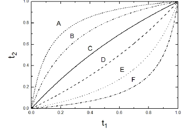
Figure 2: The transmission coefficient t₂ is altered with the t₁ to satisfy the concentration condition as shown in Eq. (15). Curve A: $\alpha^{2}$=0.1. Curve B: $\alpha^{2}$=0.2. Curve C: $\alpha^{2}$=0.4. Curve D:$\alpha^{2}$=0.5. Curve E: $\alpha^{2}$=0.8. Curve F: $\alpha^{2}$=0.9.

Here the $|1\rangle_{A}$ and $|1\rangle_{B}$ are two single photons prepared by Alice and Bob, respectively. Therefore, the two single photons combined with the $\rho_{AB}$ can be described as: with the probability of $\eta$, it is in the state $|\Psi\rangle_{a_{1}b_{1}}\otimes|1\rangle_{A}\otimes|1\rangle_{B}$, with the probability of $1-\eta$, it is in the state $|vac\rangle\otimes|1\rangle_{A}\otimes|1\rangle_{B}$. We first describe the $|\Psi\rangle_{a_{1}b_{1}}\otimes|1\rangle_{A}\otimes|1\rangle_{B}$. It evolves as

$$|\Psi\rangle_{a_{1}b_{1}}\otimes|1\rangle_{A}\otimes|1\rangle_{B}=(\alpha|1\rangle_{a1}|0\rangle_{b1}+\beta|0\rangle_{a1}|1\rangle_{b1})$$ (5)

$$\otimes |1\rangle_{A}\otimes|1\rangle_{B}\rightarrow(\alpha|1\rangle_{a1}|0\rangle_{b1}+\beta|0\rangle_{a1}|1\rangle_{b1})$$

$$\otimes (\sqrt{t_{1}}|1\rangle_{d1}|0\rangle_{d2}+\sqrt{1-t_{1}}|0\rangle_{d1}|1\rangle_{d2})$$

$$\otimes (\sqrt{t_{2}}|1\rangle_{c1}|0\rangle_{c2}+\sqrt{1-t_{2}}|0\rangle_{c1}|1\rangle_{c2})$$

$$= \alpha\sqrt{t_{1}t_{2}}|1\rangle_{a1}|0\rangle_{b1}|1\rangle_{d1}|0\rangle_{d2}|1\rangle_{c1}|0\rangle_{c2}$$

$$+ \alpha\sqrt{t_{1}(1-t_{2})}|1\rangle_{a1}|0\rangle_{b1}|1\rangle_{d1}|0\rangle_{d2}|0\rangle_{c1}|1\rangle_{c2}$$

$$+ \alpha\sqrt{t_{2}(1-t_{1})}|1\rangle_{a1}|0\rangle_{b1}|0\rangle_{d1}|1\rangle_{d2}|1\rangle_{c1}|0\rangle_{c2}$$

$$+ \alpha\sqrt{(1-t_{1})(1-t_{2})}|1\rangle_{a1}|0\rangle_{b1}|0\rangle_{d1}|1\rangle_{d2}|0\rangle_{c1}|1\rangle_{c2}$$

$$+ \beta\sqrt{t_{1}t_{2}}|0\rangle_{a1}|1\rangle_{b1}|1\rangle_{d1}|0\rangle_{d2}|1\rangle_{c1}|0\rangle_{c2}$$

$$+ \beta\sqrt{t_{1}(1-t_{2})}|0\rangle_{a1}|1\rangle_{b1}|1\rangle_{d1}|0\rangle_{d2}|0\rangle_{c1}|1\rangle_{c2}$$

$$+ \beta\sqrt{t_{2}(1-t_{1})}|0\rangle_{a1}|1\rangle_{b1}|0\rangle_{d1}|1\rangle_{d2}|1\rangle_{c1}|0\rangle_{c2}$$

$$+ \beta\sqrt{(1-t_{1})(1-t_{2})}|0\rangle_{a1}|1\rangle_{b1}|0\rangle_{d1}|1\rangle_{d2}|0\rangle_{c1}|1\rangle_{c2}.$$

In order to realize the protocol, both Alice and Bob should detect one and only one photon. From Eq. (5), terms $|1\rangle_{a1}|0\rangle_{b1}|1\rangle_{d1}|0\rangle_{d2}|1\rangle_{c1}|0\rangle_{c2}$, $|1\rangle_{a1}|0\rangle_{b1}|1\rangle_{d1}|0\rangle_{d2}|0\rangle_{c1}|1\rangle_{c2}$,$|1\rangle_{a1}|0\rangle_{b1}|0\rangle_{d1}|1\rangle_{d2}|0\rangle_{c1}|1\rangle_{c2}$, $|0\rangle_{a1}|1\rangle_{b1}|1\rangle_{d1}|0\rangle_{d2}|1\rangle_{c1}|0\rangle_{c2}$, $|0\rangle_{a1}|1\rangle_{b1}|0\rangle_{d1}|1\rangle_{d2}|1\rangle_{c1}|0\rangle_{c2}$ and $|0\rangle_{a1}|1\rangle_{b1}|0\rangle_{d1}|1\rangle_{d2}|0\rangle_{c1}|1\rangle_{c2}$ cannot lead the Alice and Bob both only detect one photon. Therefore, by choosing the cases that both Alice and Bob only detect one photon, Eq. (5) will become

$$|\Psi_{1}\rangle = \alpha\sqrt{t_{2}(1-t_{1})}|1\rangle_{a1}|0\rangle_{b1}|0\rangle_{d1}|1\rangle_{d2}|1\rangle_{c1}|0\rangle_{c2}$$ (6)

$$+ \beta\sqrt{t_{1}(1-t_{2})}|0\rangle_{a1}|1\rangle_{b1}|1\rangle_{d1}|0\rangle_{d2}|0\rangle_{c1}|1\rangle_{c2}.$$

Certainly, $|vac\rangle\otimes|1\rangle_{A}\otimes|1\rangle_{B}$ can also lead Alice and Bob both obtain one photon. In detail,

$$|vac\rangle\otimes|1\rangle_{A}\otimes|1\rangle_{B}$$ (7)

$$= |vac\rangle\otimes(\sqrt{t_{1}}|1\rangle_{d1}|0\rangle_{d2}+\sqrt{1-t_{1}}|0\rangle_{d1}|1\rangle_{d2})$$

$$\otimes (\sqrt{t_{2}}|1\rangle_{c1}|0\rangle_{c2}+\sqrt{1-t_{2}}|0\rangle_{c1}|1\rangle_{c2})$$

$$= |vac\rangle\otimes(\sqrt{t_{1}t_{2}}|1\rangle_{d1}|0\rangle_{d2}|1\rangle_{c1}|0\rangle_{c2}$$

$$+ \sqrt{(1-t_{1})t_{2}}|0\rangle_{d1}|1\rangle_{d2}|1\rangle_{c1}|0\rangle_{c2}$$

$$+ \sqrt{t_{1}(1-t_{2})}|1\rangle_{d1}|0\rangle_{d2}|0\rangle_{c1}|1\rangle_{c2}$$

$$+ \sqrt{(1-t_{1})(1-t_{2})}|0\rangle_{d1}|1\rangle_{d2}|0\rangle_{c1}|1\rangle_{c2}).$$

From Eq. (7), they will obtain

$$|\Psi_{2}\rangle=(\sqrt{t_{1}t_{2}}|1\rangle_{d1}|0\rangle_{d2}|1\rangle_{c1}|0\rangle_{c2},$$ (8)

if Alice and Bob both contain one photon. The total success probability is

$$P=\eta(\alpha^{2}t_{2}+\beta^{2}t_{1})+t_{1}t_{2}-2\eta t_{1}t_{2}.$$ (9)

In Fig. 1, the beam splitters (BSs) are used to convert

$$|1\rangle_{a1}\rightarrow\frac{1}{\sqrt{2}}(|1\rangle_{f1}+|1\rangle_{f2}),$$

$$|1\rangle_{d1}\rightarrow\frac{1}{\sqrt{2}}(|1\rangle_{f1}-|1\rangle_{f2}).$$

$$|1\rangle_{b1}\rightarrow\frac{1}{\sqrt{2}}(|1\rangle_{e1}+|1\rangle_{e2}),$$

$$|1\rangle_{c1}\rightarrow\frac{1}{\sqrt{2}}(|1\rangle_{e1}-|1\rangle_{e2}).$$ (10)

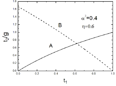
Figure 3: The transmission coefficient t₂ (Curve A) and the amplification factor g (Curve B) are altered with t₁, with $\alpha^{2}$=0.4. Here we choose $\eta=0.6$.

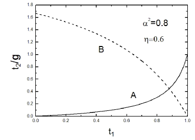
Figure 4: The transmission coefficient t₂ (Curve A) and the amplification factor g (Curve B) are altered with t₁, with $\alpha^{2}$=0.8. Here we choose $\eta=0.6$.

Therefore, if the single-photon detectors D₁D₃ or D₂D₄ register, $|\Psi_{1}\rangle$ will become

$$|\Psi_{2}\rangle^{\prime}= \alpha\sqrt{t_{2}(1-t_{1})}|1\rangle_{a1}|0\rangle_{b1}$$ (11)

$$+ \beta\sqrt{t_{1}(1-t_{2})}|0\rangle_{a1}|1\rangle_{b1}.$$

On the other hand, if D₂D₃ or D₁D₄ register, $|\Psi_{1}\rangle$ will become

$$|\Psi_{2}\rangle^{\prime\prime} = \alpha\sqrt{t_{2}(1-t_{1})}|1\rangle_{a1}|0\rangle_{b1}$$ (12)

$$- \beta\sqrt{t_{1}(1-t_{2})}|0\rangle_{a1}|1\rangle_{b1}.$$

One of the parties only needs to perform a phase-flip operation to convert it to $|\Psi_{2}\rangle^{\prime}$. $|\Psi_{2}\rangle$ always becomes the vacuum state after the two photons being detected.

Therefore, after the two photons being detected, the initial state becomes

$$\rho^{\prime}_{AB}=\eta^{\prime}|\Psi^{\prime}_{2}\rangle\langle\Psi^{\prime}_{2}|+(1-\eta^{\prime})|vac\rangle\langle vac|.$$ (13)

Here

$$\eta^{\prime}=\frac{\eta(\alpha^{2}t_{2}+\beta^{2}t_{1}-t_{1}t_{2})}{\eta(\alpha^{2}t_{2}+\beta^{2}t_{1})+t_{1}t_{2}-2\eta t_{1}t_{2}}.$$ (14)

In order to obtain the maximally entangled state, they should let

$$\frac{\alpha^{2}}{\beta^{2}}=\frac{t_{1}(1-t_{2})}{{t_{2}(1-t_{1})}}.$$ (15)

Moreover, in order to realize the linear amplification, they should make $\eta^{\prime}>\eta$. If we denote the ampliation factor $g\equiv\frac{\eta^{\prime}}{\eta}$, we can obtain

$$g=\frac{\alpha^{2}t_{2}+\beta^{2}t_{1}-t_{1}t_{2}}{\eta(\alpha^{2}t_{2}+\beta^{2}t_{1})+t_{1}t_{2}-2\eta t_{1}t_{2}}.$$ (16)

III Numerical simulation and discussion

Thus far, we have briefly explained the EALCP. From above discussion, we should require two different VBSs, while in Ref.amplification7 , two similar VBSs are used. In Eq. (15), we should adjust the coefficients t₁ and t₂ to obtain the maximally entangled state, according to the initial coefficients $\alpha$ and $\beta$. Certainly, if we choose a special case that $\alpha^{2}=\beta^{2}=\frac{1}{2}$, we can obviously obtain t₁=t₂ $\equiv$t. Moreover, according to the Eq. (16), we can get $g=\frac{1-t}{\eta+t-2\eta t}$. In this way, our results is consist with the Ref.amplification7 . The relationship between t₁ and t₂ is shown in Fig. 2. We calculated the t₂ alters with t₁ under different $\alpha^{2}$. In Fig. 2, Curve A is corresponding to $\alpha^{2}=0.1$. Curve B is corresponding to $\alpha^{2}=0.2$. Curve C is corresponding to $\alpha^{2}=0.4$. Curve D is corresponding to $\alpha^{2}=0.6$. Curve E is corresponding to $\alpha^{2}=0.8$, and Curve F is corresponding to $\alpha^{2}=0.9$. From Eq. (15), if $\alpha=\beta$, we can obtain that t₁=t₂, which is same as Ref. amplification7 . The relationship described in Fig. 2 only realizes the function of entanglement concentration. In order to increase the fidelity of the entangled state, we should let $\eta^{\prime}>\eta$.

Figure 5: The amplification factor $g$ is altered with the transmission coefficient t₁ with $\alpha^{2}=0.4$. Curve A: $\eta=0.2$. Curve B: $\eta=0.4$. Curve C: $\eta=0.6$. Curve D: $\eta=0.8$. All four curves pass through the same point $K$ with $g=1$.

Figure 6: The amplification factor $g$ is altered with the transmission coefficient t₁ with $\alpha^{2}=0.8$. Curve A: $\eta=0.2$. Curve B: $\eta=0.4$. Curve C: $\eta=0.6$. Curve D: $\eta=0.8$. All four curves pass through the same point $K$ with $g=1$. The numerical simulation of the limitation $g$ shows that it is equal to $\frac{1}{\eta}$, which is consist to the theoretical derivation.

In Fig. 3 and Fig. 4, we both calculated the t₂ and amplification factor $g$ alters with the t₁ when $\eta_{0}=0.4$, $\alpha^{2}=0.4$ and $\alpha^{2}=0.8$, respectively. In Fig. 3, Curve A is the t₂ alters with the coefficient t₁ and the Curve B is the g alters with t₁. Therefore, in order to realize the amplification, we should require $t_{1}\in(0,0.44)$, and $t_{2}\in(0,0.54)$ when $\eta=0.6$, $\alpha^{2}=0.4$. On the other hand, In Fig. 4, when $\eta=0.6$, $\alpha^{2}=0.8$, we get $t_{1}\in(0,0.63)$ and $t_{1}\in(0,0.15)$. We also calculated the $g$ alters with the different initial probability $\eta$ and $\alpha^{2}$. In Fig. 5 and Fig. 6, Curve A is relationship between t₁ and $g$ when $\eta=0.2$. Curve B is $\eta=0.4$. Curve C is $\eta=0.6$ and Curve D is $\eta=0.8$. Interestingly, as shown in Fig. 5 and Fig. 6, all four curves pass through the same point $K$, which corresponding to $\eta=1$. Actually, according to Eq. (16), if $\eta=1$, we can get $\frac{\alpha^{2}t_{2}+\beta^{2}t_{1}}{2t_{1}t_{2}}=1$. It is shown that the initial coefficient $\eta$ disappears. This is the reason that all curves pass through the same point $K$. From both Figs. 5 and 6, another interesting case is that the limitation of $g$ seems to be a constant. It changes with initial $\eta$ and has nothing to do with the initial $\alpha$ and $\beta$. From Eq. (15) and Fig. 2, $t_{2}\rightarrow 0$ when $t_{1}\rightarrow 0$. In Eq. (16), term $t_{1}t_{2}$ is the second-order infinitesimal when $t_{2}\rightarrow 0$ and $t_{1}\rightarrow 0$, which can be omitted. Therefore, we can calculate the limitation of $g$ as

$$\lim_{t_{1},t_{2}\rightarrow 0}g=\frac{\alpha^{2}t_{2}+\beta^{2}t_{1}}{\eta(\alpha^{2}t_{2}+\beta^{2}t_{1})}=\frac{1}{\eta}.$$ (17)

The numerical simulation shown in Fig. 5 and Fig. 6 is consist with the Eq. (17). It is easy to explain the limitation $g$ in Eq. (17), for the upper limit of both $\eta$ and $\eta^{\prime}$ is 1, according to Eq. (2). If the initial probability $\eta$ is 0.2, the maximally value of $g$ must be 5. In this way, the limitation of $g$ is nothing to do with the coefficient $\alpha$. We should point out that if both $t_{2}\rightarrow 0$ and $t_{1}\rightarrow 0$, from Eq. (9), the total success probability is also $P\rightarrow 0$. It reveals that it is a trade-off between the success probability $P$ and amplification $g$.

IV Possible experimental realization

Figure 7: A schematic drawing of the possible experimental realization of ELACP for single-photon entangled state.

In this section, we will briefly discuss the possible realization in experiment. The main challenge for this ELACP is to ensure the input and auxiliary photons are indistinguishable in every degree of freedom. They are essentially the Hong-Ou-Mandel (HOM) interference on two BSs. As shown in Fig. 7, the pump pulse of ultraviolet light passes through a $\beta$-barium borate crystal (BBO). Then a correlated pair of photons will be generated with the probability $p$ in the spatial modes $a_{0}$ and $b_{0}$. The pump pulse of ultraviolet light will be reflected by the mirror (M) and pass through the BBO crystal in a second time, which can generate another correlated pair in the spatial mode $b_{1}$ and $b_{2}$. The position of the mirror can be adjusted. The Delay line can also be used to ensure the photons arriving at the two BSs simultaneously. The photon in the spatial mode $b_{0}$ is blocked. The photon in the spatial mode $a_{0}$ is used to prepare the initial state as shown in Eq. (2). The VBS₁ is to generate the less-entangled state $|\Psi\rangle$, similar to Ref. amplification7 . The coefficient $\alpha$ is decided by the transmission of VBS₁. The VBS₂ and VBS₃ with the same transmission are used to prepare the local bosonic lossy channels. The transmission coefficients of VBS₂ and VBS₃ is $T_{0}=\eta$. The two auxiliary photons are prepared in the spatial modes b₁ and b₂, respectively. According to the initial $\eta$ and $\alpha$, we should adjust the transmission of VBS₄ and VBS₅ to satisfy the relationship in Eqs. (15) and (16), for its realization in the experiment. On the other hand, the phase fluctuations and multi-photon cases may disturb the experiment. Fortunately, as pointed out by Refs. purification1 ; purification2 , the good overlap on the PBS and phase stability have been achieved in current experimental condition. The second problem can be solved by four-mode cases, similar as Ref.purification2 . That is the spatial modes b₀, D₁, D₃ and Out1, or b₀, D₁, D₃ and Out2 all exactly contain one photon.

V conclusion

In conclusion, we have a practical way to distill the SPE from photon loss and decoherence. By adjusting the transmission coefficients t₁ and t₂, one can both realize the amplification and concentration of the single-photon entangled state. We discussed the numerical condition of amplification factor $g$ changed with the initial parameters $\alpha$ and $\eta$. Interestingly, the limitation $g$ only depends on the $\eta$ and it has nothing to do with $\alpha$. We also discussed its possible realization in current experimental condition. Compared with the protocol of SPE amplification, this protocol is more practical. As the SEM is of vice importance in current long-distance quantum communication, this protocol is useful.

References

- (1) M. A. Nielsen and I.L. Chuang, (Cambridge University Press, Cambridge, UK, 2000).
- (2) N. Gisin, G. Ribordy, W. Tittel, and H. Zbinden, Rev. Mod. Phys. 74, 145 (2002).
- (3) A. K. Ekert, Phys. Rev. Lett. 67, 661 (1991).
- (4) G.-L. Long, and X.-S. Liu, Phys. Rev. A 65, 032302 (2002).
- (5) C. H. Bennett, G. Brassard, C. Crepeau, R. Jozsa, A. Peres, and W. K. Wootters, Phys. Rev. Lett. 70, 1895 (1993).
- (6) A. Karlsson, M. Bourennane, Phys. Rev. A 58, 4394 (1998).
- (7) F. G. Deng, C. Y. Li, Y. S. Li, H. Y. Zhou, and Y. Wang, Phys. Rev. A 72, 022338 (2005).
- (8) M. Hillery, V. Bužek, and A. Berthiaume, Phys. Rev. A 59, 1829 (1999).
- (9) A. Karlsson, M. Koashi, and N. Imoto, Phys. Rev. A 59, 162 (1999).
- (10) L. Xiao, G.-L. Long, F.-G. Deng, and J.-W. Pan, Phys. Rev. A 69, 052307 (2004).
- (11) F.-G. Deng, G.-L. Long, and X.-S. Liu, Phys. Rev. A, 68, 042317 (2003).
- (12) C. Wang, F. G. Deng, Y. S. Li, X. S. Liu, and G. L. Long, Phys. Rev. A 71, 044305 (2005).
- (13) R. Cleve, D. Gottesman, and H. K. Lo, Phys. Rev. Lett. 83, 648 (1999).
- (14) A. M. Lance, T. Symul, W. P. Bowen, B. C. Sanders, and P. K. Lam, Phys. Rev. Lett. 92, 177903 (2004).
- (15) F. G. Deng, X. H. Li, C. Y. Li, P. Zhou, and H. Y. Zhou, Phys. Rev. A 72, 044301 (2005).
- (16) S. M. Tan, D. F. Walls, and M. J. Collett, Phys. Rev. Lett. 66, 252 (1991).
- (17) L. Hardy, Phys. Rev. Lett.73, 2279 (1994).
- (18) A. Peres, Phys. Rev. Lett. 74, 4571 (1995).
- (19) C. Silberhorn, T. C. Ralph, N. Lütkenhaus, and G. Leuchs, Phys. Rev. Lett.89, 167901 (2002).
- (20) C. Silberhorn, N. Korolkova, and G. Leuchs, Phys. Rev. Lett. 88, 167902 (2002).
- (21) M. G. A. Paris, M. Cola, and R. Bonifacio, Phys. Rev. A 67, 042104 (2003).
- (22) G. M. D Ariano and P. Lo Presti, Phys. Rev. Lett. 86, 4195 (2001).
- (23) G. M. D Ariano, P. Lo Presti, and M. G. A. Paris, Phys. Rev. Lett. 87, 270404 (2001).
- (24) L. M. Duan, M. D. Lukin, J. T. Cirac and P. Zoller, Nature (London) 414, 413 (2001).
- (25) C. Simon, H. de Riedmatten, M. Afzelius, N. Sangouard, H. Zbinden, N. Gisin, Phys. Rev. Lett. 98, 190503 (2007).
- (26) N. Sangouard, C. Simon, B. Zhao, Y. A. Chen, H. de Riedmatten, J. W. Pan, and N. Gisin, Phys. Rev. A 77, 062301 (2008).
- (27) N. Sangouard, C. Simon, H. de Riedmatten, and N. Gisin, Rev. Mod. Phys. 83, 33 (2011).
- (28) N. Sangouard, C. Simon, T. Coudreau, and N. Gisin, Phys. Rev. A 78, 050301 (2008).
- (29) D. Salart, O. Landry, N. Sangouard, N. Gisin, H. Herrmann, B. Sanguinetti, C. Simon, W. Sohler, R. T. Thew, A. Thomas, H. Zbinden, Phys. Rev. Lett. 104, 180504 (2010).
- (30) Y. B. Sheng, F. G. Deng, and H. Y. Zhou, Quant. Inf. & Comput. 10, 272 (2010).
- (31) L. Zhou, Y. B. Sheng, W. W. Cheng, L. Y. Gong and S. M. Zhao, J. Opt. Soc. Am. B 30, 71 (2013).
- (32) G. S. Paraoanu, Found Phys. 41, 1214 (2011).
- (33) G. S. Paraoanu, Phys. Rev. A 83, 044101 (2011).
- (34) G. S. Paraonau, Eur. Phys. Lett. 93, 64002 (2011).
- (35) T. C. Ralph, and A. P. Lund, in Quantum Communication Measurement and Computing, Proceedings of 9th International Conference, edited by A. lvovsky (AIP, New York, 2009) pp. 155-160.
- (36) N. Gisin, S. Pironio, and N. Sangouard, Phys. Rev. Lett. 105, 070501 (2010).
- (37) G. Y. Xiang, T. C. Ralph, A. P. Lund, N. Walk, and G. J. Pryde, Nat. Photon. 4, 316 (2010).
- (38) M. Curty, and T. Moroder, Phys. Rev. A 84, 010304(R) (2011).
- (39) D. Pitkanen, X. Ma, R. Wickert, P. van Loock, and N. Lütkenhaus, Phys. Rev. A 84, 022325 (2011).
- (40) C. I. Osorio, N. Bruno, N. Sangouard, H. Zbinden, N. Gisin, and R. T. Thew, Phys. Rev. A 86, 023815 (2012).
- (41) S. Kocsis, G. Y. Xiang, T. C. Ralph, and G. J. Pryde, Nat. Phys. 9, 23 (2013).
- (42) S. L. Zhang, S. Yang, X. B. Zou, B. S. Shi, and G. C. Guo, Phys. Rev. A 86, 034302 (2012).
- (43) C. H. Bennett, H. J. Bernstein, S. Popescu, and B. Schumacher, Phys. Rev. A 53, 2046 (1996).
- (44) S. Bose, V. Vedral, and P. L. Knight, Phys. Rev A 60, 194 (1999).
- (45) B. S. Shi, Y. K. Jiang, and G. C. Guo, Phys. Rev. A 62, 054301 (2000).
- (46) Z. Zhao, J. W. Pan, and M. S. Zhan, Phys. Rev. A 64, 014301 (2001).
- (47) T. Yamamoto, M. Koashi, and N. Imoto, Phys. Rev. A 64, 012304 (2001).
- (48) Y. B. Sheng, F. G. Deng, and H. Y. Zhou, Phys. Rev. A 77, 062325 (2008).
- (49) Y. B. Sheng, L. Zhou, S. M. Zhao, and B. Y. Zheng, Phys. Rev. A 85, 012307 (2012).
- (50) F. G. Deng, Phys. Rev. A 85, 022311 (2012).
- (51) C. Wang, Y. Zhang and G. S. Jin, Phys. Rev. A 84, 032307 (2011).
- (52) C. Wang, Phys. Rev. A 86, 012323 (2012).
- (53) L. Zhou, Y. B. Sheng, W. W. Cheng, G. L. Yan, and S. M. Zhao, Quant. Inf. Process. 12, 1307 (2013).
- (54) Y. B. Sheng, and L. Zhou, Entropy, 15, 1776 (2013).
- (55) Y. B. Sheng, L. Zhou, and S. M. Zhao, Phys. Rev. A 85, 042302 (2012).
- (56) C. Simon, and J. W. Pan, Phys. Rev. Lett. 89, 257901 (2002).
- (57) J. W. Pan, C. Simon, C̆. Brukner, and A. Zeilinger, Nature 410, 1067 (2001).