An efficient spectral method for computing dynamics of rotating two-component Bose–Einstein condensates via coordinate transformation

Abstract

In this paper, we propose an efficient and accurate numerical method for computing the dynamics of rotating two-component Bose–Einstein condensates (BECs) which is described by coupled Gross–Pitaevskii equations (CGPEs) with an angular momentum rotation term and an external driving field. By introducing rotating Lagrangian coordinates, we eliminate the angular momentum rotation term from the CGPEs, which allows us to develop an efficient numerical method. Our method has spectral accuracy in all spatial dimensions and moreover it can be easily implemented in practice. To examine its performance, we compare our method with those reported in literature. Numerical results show that to achieve the same accuracy, our method needs much shorter computing time. We also applied our method to study the dynamic properties of rotating two-component BECs. Furthermore, we generalize our method to solve the vector Gross–Pitaevskii equations (VGPEs) which is used to study rotating multi-component BECs.

1 Introduction

The Bose–Einstein condensation (BEC), which affords an astonishing glimpse into the macroscopic quantum world, has been extensively studied since its first realization in 1995 [2, 15, 20]. Later, with the observation of quantized vortices in BECs [36, 37], attention has been broaden to explore vortex states and their dynamics associated with superfluidity. Rotating BECs which are known to exhibit highly regular vortex lattices have been heavily studied both experimentally and theoretically [1, 38, 33, 21]. On the other hand, multi-component BECs admit numerous interesting phenomena absent from single-component condensates, for example, domain walls, vortons, square vortex lattices and so on; see [24, 25, 18, 27, 29, 31, 32] and references therein. As the simplest cases, two-component BECs provide a good opportunity to investigate the properties of multi-component condensation.

The first experiment of two-component BECs was carried out in $|F=2,m_{f}=2\rangle$ and $|F=1,m_{f}=-1\rangle$ hyperfine states of ${}^{87}{\rm Rb}$ [39]. At temperatures $T$ much smaller than the critical temperature $T_{c}$, a rotating two-component BEC with an external driving field (or an internal Josephson junction) can be well described by two self-consistent nonlinear Schrödinger equations (NLSEs), also known as the coupled Gross–Pitaevskii equations (CGPEs). The dimensionless CGPEs has the following form [30, 31, 43, 44, 10, 12, 32]:

$$i\frac{\partial\psi_{1}({\bf x},t)}{\partial t}=\left[-\frac{1}{2}\nabla^{2}+V_{1}({\bf x})+(\beta_{11}|\psi_{1}|^{2}+\beta_{12}|\psi_{2}|^{2})-\Omega L_{z}\right]\psi_{1}-\lambda\psi_{2},$$ (1.1)

$$i\frac{\partial\psi_{2}({\bf x},t)}{\partial t}=\left[-\frac{1}{2}\nabla^{2}+V_{2}({\bf x})+(\beta_{21}|\psi_{1}|^{2}+\beta_{22}|\psi_{2}|^{2})-\Omega L_{z}\right]\psi_{2}-\lambda\psi_{1},\quad{\bf x}\in{\mathbb{R}}^{d},\ \,t>0.\qquad\quad$$ (1.2)

Here, ${\bf x}\in{\mathbb{R}}^{d}$ ($d=2$ or $3$) is the Cartesian coordinate vector, $t$ is the time and $\psi_{j}({\bf x},t)$ is the complex-valued macroscopic wave function of the $j$th ($j=1,2$) component. The interaction constants $\beta_{jk}=\beta_{kj}={4\pi Na_{jk}}/{a_{0}}$ (for $j,k=1,2$), where $N$ is the total number of atoms in two-component BECs, $a_{0}$ is the dimensionless spatial unit and $a_{jk}=a_{kj}$ represents the $s$-wave scattering lengths between the $j$th and $k$th components (positive for repulsive interaction and negative for attractive interaction). The constant $\lambda$ describes the effective Rabi frequency to realize the internal atomic Josephson junction by a Raman transition, $\Omega$ represents the speed of angular momentum rotation and $L_{z}=-i(x\partial_{y}-y\partial_{x})$ is the $z$-component of the angular momentum operator. The real-valued function $V_{j}({\bf x})$ ($j=1,2$) represents the external trapping potential imposed on the $j$th component. In most BEC experiments, a harmonic potential is used, i.e.,

$$V_{j}({\bf x})=\frac{1}{2}\left\{\begin{array}[]{ll}{\gamma}_{x,j}^{2}x^{2}+{\gamma}_{y,j}^{2}y^{2},&d=2,\\ {\gamma}_{x,j}^{2}x^{2}+{\gamma}_{y,j}^{2}y^{2}+{\gamma}_{z,j}^{2}z^{2},&d=3,\end{array}\right.\quad\ \ j=1,2.$$ (1.5)

The initial conditions of (1.1)–(1.2) are given by

$$\psi_{j}({\bf x},0)=\psi_{j}^{0}({\bf x}),\quad\ {\bf x}\in{\mathbb{R}}^{d},\quad\ \ j=1,2.$$ (1.6)

There are two important invariants associated with the CGPEs in (1.1)–(1.2): the total mass (or normalization), i.e.,

$$N(t):=\|\Psi(\cdot,t)\|^{2}=N_{1}(t)+N_{2}(t)\equiv\|\Psi(\cdot,0)\|^{2}=1,\quad\ t\geq 0,$$ (1.7)

where $\Psi({\bf x},t)=(\psi_{1}({\bf x},t),\psi_{2}({\bf x},t))^{T}$ and $N_{j}$(t) is the mass of the $j$th component at time $t\geq 0$, which is defined by

$$N_{j}(t):=\|\psi_{j}(\cdot,t)\|^{2}=\int_{{\mathbb{R}}^{d}}|\psi_{j}({\bf x},t)|^{2}d{\bf x},\quad\ t\geq 0,\quad\ \ j=1,2,$$ (1.8)

and the energy

$$E(\Psi(\cdot,t)) = \int_{{\mathbb{R}}^{d}}\bigg{[}\sum_{j=1}^{2}\bigg{(}\frac{1}{2}|\nabla\psi_{j}|^{2}+V_{j}({\bf x})|\psi_{j}|^{2}+\frac{\beta_{jj}}{2}|\psi_{j}|^{4}-\Omega{\rm Re}\left(\psi_{j}^{*}L_{z}\psi_{j}\right)\bigg{)}\qquad$$ (1.9)

$$\qquad+\beta_{12}|\psi_{1}|^{2}|\psi_{2}|^{2}-2\lambda{\rm Re}(\psi_{1}\psi_{2}^{*})\bigg{]}d{\bf x}=E(\Psi(\cdot,0)),\quad\ t\geq 0,$$

where ${\rm Re}(f)$ and $f^{*}$ represent the real part and the conjugate of a function $f$, respectively. In fact, if there is no external driving filed (i.e., $\lambda=0$ in (1.1)–(1.2)), the mass of each component is also conserved, i.e., $N_{j}(t)=N_{j}(0)$ ($j=1,2$) for $t\geq 0$. These invariants can be used, in particular, as benchmarks and validation of numerical algorithms for solving the CGPEs (1.1)–(1.2).

Many numerical methods have been proposed to study the dynamics of the non-rotating two-component BECs, i.e., when $\Omega=0$, with/without external driving field [5, 40, 45, 17]. Compared to other methods, the time-splitting pseudo-spectral method in [5] is one of the most successful methods. It has spectral order of accuracy in space and can be easily implemented, i.e., they can achieve both the accuracy and efficiency. However, the appearance of the angular rotational term hinders the direct application of those methods to study the rotating two-component BECs. Recently, several numerical methods were proposed for simulating the dynamics of rotating two-component BECs [44, 43, 10, 19, 26, 28]. For example, in [44], a pseudo-spectral type method was proposed by reformulating the problem in two-dimensional polar coordinates or three-dimensional cylindrical coordinates. While in [43], the authors designed a time-splitting alternating direction implicit method, where the angular rotation term is treated in $x$- and $y$-directions separately. Although these methods have higher spatial accuracy compared to those finite difference/element methods, they have their own limitations. The method in [44] is only of second-order or fourth-order in the radial direction, while the implementation of the method in [43] could become quite involved. One possible approach to overcome those limitations is to relax the constrain of the rotational term, which is the main aim of this paper. In this paper, we propose a simple and efficient numerical method to solve the CGPEs (1.1)–(1.2). The main merits of our method are: (i) Using a rotating Lagrangian coordinate transform, we reformulate the original CGPEs in (1.1)–(1.2) to one without angular momentum rotation term. Then, the time-splitting pseudo-spectral method designed for the non-rotating BECs, which are of spectral order accuracy in space and easy to implemented, can be directly applied to solve the CGPEs in new coordinates. Moreover, (ii) our method solves the CGPEs in two splitting steps instead of three steps in literature [44, 43], which makes our method more efficient.

The paper is organized as follows. In Section 2, we introduce a rotating Lagrangian coordinate and then cast the CGPEs (1.1)–(1.6) in the new coordinate system. A simple and efficient numerical method is introduced to discretize the CGPEs under a rotating Lagrangian coordinate in Section 3, which is subsequently generalized in Section 4 to solve the VGPEs for multi-component BECs. To test its performance, we compare our method with those reported in literature and apply it to study the dynamics of rotating two-component BECs in Section 5. In Section 6, we make some concluding remarks.

2 CGPEs under a rotating Lagrangian coordinate

In this section, we first introduce a rotating Lagrangian coordinate and then reformulate the CGPEs (1.1)–(1.6) in the new coordinate system. In the following, we will always refer the Cartesian coordinates ${\bf x}$ as the Eulerian coordinates. For any time $t\geq 0$, let ${\bf A}(t)$ be an orthogonal rotational matrix defined as [22, 4, 13]

$${\bf A}(t)=\left(\begin{array}[]{cc}\cos(\Omega t)&\sin(\Omega t)\\ -\sin(\Omega t)&\cos(\Omega t)\end{array}\right),\quad\ \ \mbox{if \ \ $d=2$,}\qquad\quad\ \$$ (2.3)

and

$${\bf A}(t)=\left(\begin{array}[]{ccc}\cos(\Omega t)&\sin(\Omega t)&0\\ -\sin(\Omega t)&\cos(\Omega t)&0\\ 0&0&1\end{array}\right),\quad\ \ \mbox{if \ \ $d=3$.}\qquad$$ (2.7)

It is easy to verify that ${\bf A}^{-1}(t)={\bf A}^{T}(t)$ for any $t\geq 0$ and ${\bf A}(0)={\bf I}$ with ${\bf I}$ the identity matrix. Referring the Cartesian coordinates ${\bf x}$ as the Eulerian coordinates, we introduce the rotating Lagrangian coordinates $\widetilde{\bf x}$ as

$$\widetilde{\bf x}={\bf A}^{-1}(t){\bf x}={\bf A}^{T}(t){\bf x}\quad\Leftrightarrow\quad{\bf x}={\bf A}(t){\widetilde{\bf x}},\quad\ {\bf x}\in{\mathbb{R}}^{d},\quad t\geq 0.$$ (2.8)

and reformulate the wave functions $\psi_{j}({\bf x},t)$ in the new coordinates as $\phi_{j}(\widetilde{\bf x},t)$

$$\phi_{j}(\widetilde{\bf x},t):=\psi_{j}({\bf x},t)=\psi_{j}\left({\bf A}(t){\widetilde{\bf x}},t\right),\quad\ \widetilde{\bf x}\in{\mathbb{R}}^{d},\quad t\geq 0,\quad\ \ j=1,2.$$ (2.9)

We see that when $d=3$, the transformation in (2.8) does not change the coordinate in $z$-direction, that is, $\widetilde{z}=z$ and the coordinate transformation essentially occurs only in $xy$-plane for any $t\geq 0$. Fig. 1 illustrates the geometrical relation between the $xy$-plane in the Eulerian coordinates and $\tilde{x}\tilde{y}$-plane in the rotating Lagrangian coordinates for $\Omega>0$.

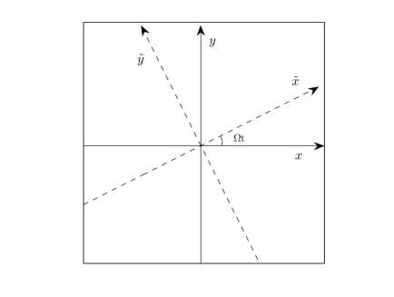
Figure 1: Eulerian (or Cartesian) coordinates $(x,y)$ (solid) and rotating Lagrangian coordinates $(\tilde{x},\tilde{y})$ (dashed) in two dimensions for $\Omega>0$ at a fixed $t\geq 0$.

Furthermore, it is easy to see that when $t=0$ the rotating Lagrangian coordinates $\widetilde{\bf x}$ become exactly the same as the Eulerian coordinates ${\bf x}$, i.e., $\widetilde{\bf x}\equiv{\bf x}$ when $t=0$. Note that we assume that $\Omega\neq 0$ in this paper.

From (2.8)–(2.9), we obtain that

$$\partial_{t}\phi_{j}(\widetilde{\bf x},t)=\partial_{t}\psi_{j}({\bf x},t)+\nabla\psi_{j}({\bf x},t)\cdot\left(\dot{\bf A}(t)\widetilde{\bf x}\right)=\partial_{t}\psi_{j}({\bf x},t)-\Omega(x\partial_{y}-y\partial_{x})\psi_{j}({\bf x},t),\qquad\quad$$

$$\nabla\phi_{j}(\widetilde{\bf x},t)={{\bf A}^{-1}}(t)\nabla\psi_{j}({\bf x},t),\quad\nabla^{2}\phi_{j}(\widetilde{\bf x},t)=\nabla^{2}\psi_{j}({\bf x},t),\quad\ {\bf x}\in{\mathbb{R}}^{d},\quad t\geq 0,\quad\ j=1,2.$$

Substituting the above derivatives into (1.1)–(1.2) gives the following $d$-dimensional CGPEs in the rotating Lagrangian coordinates $\widetilde{\bf x}$:

$$i\frac{\partial\phi_{1}(\widetilde{{\bf x}},t)}{\partial t}=\left[-\frac{1}{2}\nabla^{2}+W_{1}(\widetilde{{\bf x}},t)+(\beta_{11}|\phi_{1}|^{2}+\beta_{12}|\phi_{2}|^{2})\right]\phi_{1}-\lambda\phi_{2},\qquad\qquad$$ (2.10)

$$i\frac{\partial\phi_{2}(\widetilde{{\bf x}},t)}{\partial t}=\left[-\frac{1}{2}\nabla^{2}+W_{2}(\widetilde{{\bf x}},t)+(\beta_{21}|\phi_{1}|^{2}+\beta_{22}|\phi_{2}|^{2})\right]\phi_{2}-\lambda\phi_{1},\quad\ \widetilde{\bf x}\in{\mathbb{R}}^{d},\quad t>0.\qquad\qquad$$ (2.11)

The corresponding initial conditions are

$$\phi_{j}(\widetilde{\bf x},0):=\phi_{j}^{0}(\widetilde{\bf x})=\psi_{j}({\bf x},0)=\psi_{j}^{0}({\bf x}),\quad\ \widetilde{\bf x}={\bf x}\in{\mathbb{R}}^{d}.$$ (2.12)

In (2.10)–(2.11), $W_{j}(\widetilde{\bf x},t)$ ($j=1,2$) denotes the effective potential of the $j$th component, which is obtained from

$$W_{j}(\widetilde{\bf x},t)=V_{j}(A(t)\widetilde{\bf x}),\quad\ \widetilde{\bf x}\in{\mathbb{R}}^{d},\quad t\geq 0,\quad\ \ j=1,2.$$ (2.13)

In particular, if $V_{j}({\bf x})$ is a harmonic potential as defined in (1.5), then $W_{j}(\widetilde{\bf x},t)$ has the form

$$W_{j}(\widetilde{\bf x},t)$$

$$\quad=\frac{{\gamma}_{x,j}^{2}+{\gamma}_{y,j}^{2}}{4}(\widetilde{x}^{2}+\widetilde{y}^{2})+\frac{{\gamma}_{x,j}^{2}-{\gamma}_{y,j}^{2}}{4}\left[(\widetilde{x}^{2}-\widetilde{y}^{2})\cos(2\Omega t)+2\widetilde{x}\widetilde{y}\sin(2\Omega t)\right]+\left\{\begin{array}[]{ll}0&d=2,\\ \frac{1}{2}{\gamma}_{z,j}^{2}\widetilde{z}^{2},&d=3,\\ \end{array}\right.\qquad$$

for $j=1,2$. Hence, when the external harmonic potentials are radially symmetric in two dimensions (2D) or cylindrically symmetric in three dimensions (3D), i.e., ${\gamma}_{x,j}={\gamma}_{y,j}:={\gamma}_{r,j}$, the potential

$$W_{j}(\widetilde{\bf x},t)=V_{j}(\widetilde{\bf x}),\quad\ \widetilde{\bf x}\in{\mathbb{R}}^{d},\quad t\geq 0,\quad\ j=1,2,$$ (2.15)

become time-independent.

In rotating Lagrangian coordinates, the wave functions $\Phi(\widetilde{\bf x},t)=(\phi_{1}(\widetilde{\bf x},t),\phi_{2}(\widetilde{\bf x},t))^{T}$ satisfy the normalization

$${\widetilde{N}}(t):=\|\Phi(\cdot,t)\|^{2}={\widetilde{N}}_{1}(t)+{\widetilde{N}}_{2}(t)\equiv\|\Phi(\cdot,0)\|^{2}=1,\quad\ t\geq 0,$$ (2.16)

where ${\widetilde{N}}_{j}(t)$ is the mass of the $j$th component at time $t\geq 0$, i.e.,

$$\widetilde{N}_{j}(t):=\|\phi_{j}(\cdot,t)\|^{2}=\int_{{\mathbb{R}}^{d}}|\phi_{j}(\widetilde{\bf x},t)|^{2}d\widetilde{\bf x}=N_{j}(t),\quad t\geq 0,\quad\ \ j=1,2.$$ (2.17)

Similarly, when $\lambda=0$ the mass of each component is also conserved, i.e., $\widetilde{N}_{j}(t)\equiv\widetilde{N}_{j}(0)$ for $t\geq 0$ and $j=1,2$. The energy associated with the CGPEs (2.10)–(2.11) is

$$\widetilde{E}(\Phi(\cdot,t))=\int_{{\mathbb{R}}^{d}}\bigg{[}\sum_{j=1}^{2}\bigg{(}\frac{1}{2}|\nabla\phi_{j}|^{2}+W_{j}(\widetilde{\bf x},t)|\phi_{j}|^{2}-\int_{0}^{t}|\phi_{j}|^{2}\partial_{\tau}W_{j}(\widetilde{\bf x},\tau)d\tau+\frac{\beta_{jj}}{2}|\phi_{j}|^{4}\bigg{)}$$

$$\qquad\qquad\qquad\quad\ \ +\beta_{12}|\phi_{1}|^{2}|\phi_{2}|^{2}-2\lambda{\rm Re}(\phi_{1}\phi_{2}^{*})\bigg{]}d\widetilde{\bf x}=\widetilde{E}(\Phi(\cdot,0)),\quad\ t\geq 0.$$ (2.18)

As we see in (2.15), when ${\gamma}_{x,j}={\gamma}_{y,j}$ ($j=1,2$), the potential $W_{j}(\widetilde{\bf x},t)$ is time-independent, which implies that the term of $\int_{0}^{t}|\phi_{j}|^{2}\partial_{\tau}W_{j}(\widetilde{\bf x},\tau)d\tau\equiv 0$ in this case.

Compared to (1.1)–(1.2), the CGPEs (2.10)–(2.11) in rotating Lagrangian coordinates does not have the angular momentum rotational term, which eliminates the difficulties in discretizing the CGPEs and allows us to develop an efficient spectral method to solve (2.10)–(2.11).

3 Numerical method

In this section, we present a time-splitting spectral method to study the dynamics of rotating two-component BECs. To the best of our knowledge, so far all numerical methods computing dynamics of rotating two-component BECs in literature are based on discretizing the CGPEs (1.1)–(1.2) in Eulerian coordinates [44, 43, 10]. However, the appearance of rotating angular momentum term in Eulerian coordinates makes it very challenging to develop an efficient methods with higher accuracy but less computational efforts. In the following, instead of simulating (1.1)–(1.2) in Eulerian coordinates, we solve the CGPEs (2.10)–(2.11) in rotating Lagrangian coordinates. Hence, we avoid the discretization of the angular rotational term and it makes numerical method simpler and more efficient than those reported in [43, 44].

In practical computations, we truncate the problem (2.10)–(2.11) into a bounded computational domain ${\mathcal{D}}\subset{\mathbb{R}}^{d}$ and consider

$$i\partial_{t}\phi_{1}(\widetilde{{\bf x}},t)=\left[-\frac{1}{2}\nabla^{2}+W_{1}(\widetilde{{\bf x}},t)+(\beta_{11}|\phi_{1}|^{2}+\beta_{12}|\phi_{2}|^{2})\right]\phi_{1}-\lambda\phi_{2},\qquad\qquad$$ (3.1)

$$i\partial_{t}\phi_{2}(\widetilde{{\bf x}},t)=\left[-\frac{1}{2}\nabla^{2}+W_{2}(\widetilde{{\bf x}},t)+(\beta_{21}|\phi_{1}|^{2}+\beta_{22}|\phi_{2}|^{2})\right]\phi_{2}-\lambda\phi_{1},\quad\ \widetilde{\bf x}\in{\mathcal{D}},\quad t>0,\qquad\qquad$$ (3.2)

along with the initial conditions

$$\phi_{j}(\widetilde{\bf x},t)=\phi_{j}^{0}(\widetilde{\bf x}),\quad\ \widetilde{\bf x}\in\overline{\mathcal{D}},\qquad\mbox{with}\quad\int_{\overline{\mathcal{D}}}\left(|\phi_{1}^{0}(\widetilde{\bf x})|^{2}+|\phi_{2}^{0}(\widetilde{\bf x})|^{2}\right)d\widetilde{\bf x}=1.$$ (3.3)

The following homogeneous Dirichlet boundary conditions are considered here, i.e.,

$$\phi_{j}(\widetilde{\bf x},t)=0,\quad\ \widetilde{\bf x}\in\partial{\mathcal{D}},\quad t>0,\quad\ \ j=1,2.$$ (3.4)

Due to the confinement of the external potential $W_{j}({\bf x},t)$ and conservation of the normalization (2.16) and energy (2), the wave function $\phi_{j}(\widetilde{\bf x},t)$ vanishes as $|\widetilde{\bf x}|\rightarrow\infty$. Hence, it is natural to impose homogeneous Dirichlet boundary conditions to the truncated problem (3.1)–(3.3). The use of more sophisticated boundary conditions for more generalized cases, e.g., absence of trapping potential, is an interesting topic that remains to be examined in the future [3, 6]. In practical simulations, the computational domain ${\mathcal{D}}\subset{\mathbb{R}}^{d}$ is chosen as ${\mathcal{D}}=[a,b]\times[c,e]$ if $d=2$ and ${\mathcal{D}}=[a,b]\times[c,e]\times[f,g]$ if $d=3$. Moreover, we use sufficiently large domain ${\mathcal{D}}$ to ensure the homogeneous Dirichlet boundary conditions do not introduce aliasing error. Usually, the diameter of the bounded computational domain depends on the problem. In general, it should be larger than the “Thomas-Fermi radius” [7, 8].

3.1 Time-splitting method

In the following, we use the time-splitting method to discretize the problem (3.1)–(3.4) in time. To do it, we choose a time step $\Delta t>0$ and define time sequence $t_{n}=n\Delta t$ for $n=0,1,\ldots$. Then from time $t=t_{n}$ to $t=t_{n+1}$, we numerically solve the CGPEs (3.1)–(3.2) in two steps, i.e., solving

$$i\frac{\partial\phi_{j}(\widetilde{\bf x},t)}{\partial t}=-\frac{1}{2}\nabla^{2}\phi_{j}(\widetilde{\bf x},t)-\lambda\phi_{(3-j)}(\widetilde{\bf x},t),\quad\ \widetilde{\bf x}\in{\mathcal{D}},\quad t_{n}\leq t\leq t_{n+1},\quad\ \ j=1,2,$$ (3.5)

and

$$i\frac{\partial\phi_{j}(\widetilde{\bf x},t)}{\partial t}=\Big{(}W_{j}(\widetilde{\bf x},t)+\sum_{k=1}^{2}\beta_{jk}|\phi_{k}|^{2}\Big{)}\phi_{j}(\widetilde{\bf x},t),\quad\ \widetilde{\bf x}\in{\mathcal{D}},\quad t_{n}\leq t\leq t_{n+1},\quad\ \ j=1,2.$$ (3.6)

In fact, Eq. (3.5) is coupled linear Schrödinger equations and its discretization will be discussed later.

We notice that in (3.6), both $|\phi_{1}(\widetilde{\bf x},t)|$ and $|\phi_{2}(\widetilde{\bf x},t)|$ are invariants in time $t$, i.e., $|\phi_{j}(\widetilde{\bf x},t)|=|\phi_{j}(\widetilde{\bf x},t_{n})|$ ($j=1,2$) for any $t\in[t_{n},t_{n+1}]$. Thus, for time $t\in[t_{n},t_{n+1}]$, (3.6) is equivalent to

$$i\partial_{t}\phi_{j}(\widetilde{\bf x},t)=\Big{(}W_{j}(\widetilde{\bf x},t)+\sum_{k=1}^{2}\beta_{jk}|\phi_{k}(\widetilde{\bf x},t_{n})|^{2}\Big{)}\phi_{j}(\widetilde{\bf x},t),\quad\ \widetilde{\bf x}\in{\mathcal{D}},\quad\ \ j=1,2.$$ (3.7)

Integrating (3.7) exactly in time leads to the solution of (3.6), i.e.,

$$\phi_{j}(\widetilde{\bf x},t)=\phi_{j}(\widetilde{\bf x},t_{n})\exp\Big{[}-i\Big{(}(t-t_{n})\sum_{k=1}^{2}\beta_{jk}|\phi_{k}(\widetilde{\bf x},t_{n})|^{2}+\int_{t_{n}}^{t}W_{j}(\widetilde{\bf x},\tau)d\tau\Big{)}\Big{]},\quad\ \ j=1,2,$$ (3.8)

for $\widetilde{\bf x}\in{\mathcal{D}}$ and $t\in[t_{n},t_{n+1}]$.

Remark 3.1.

If $V_{j}({\bf x})$ ($j=1,2)$ is a harmonic potential as defined in (1.5), then the integral in (3.8) can be evaluated analytically, i.e.,

$$\int_{t_{n}}^{t}W_{j}(\widetilde{\bf x},\tau)d\tau=\frac{({\gamma}_{x,j}^{2}+{\gamma}_{y,j}^{2})(\widetilde{x}^{2}+\widetilde{y}^{2})}{4}(t-t_{n})+U(\widetilde{\bf x},t)+\left\{\begin{array}[]{ll}0,&d=2,\\ \frac{1}{2}{\gamma}_{z,j}^{2}\widetilde{z}^{2}(t-t_{n}),&d=3,\end{array}\right.$$ (3.11)

where

$$U(\widetilde{\bf x},t) = \frac{({\gamma}_{x,j}^{2}-{\gamma}_{y,j}^{2})}{4}\int_{t_{n}}^{t}\left[(\widetilde{x}^{2}-\widetilde{y}^{2})\cos(2\Omega\tau)+2\widetilde{x}\widetilde{y}\sin(2\Omega\tau)\right]d\tau$$

$$= \frac{({\gamma}_{x,j}^{2}-{\gamma}_{y,j}^{2})(\widetilde{x}^{2}-\widetilde{y}^{2})}{8\Omega}[\sin(2\Omega t)-\sin(2\Omega t_{n})]-\frac{({\gamma}_{x,j}^{2}-{\gamma}_{y,j}^{2})\widetilde{x}\widetilde{y}}{4\Omega}[\cos(2\Omega t)-\cos(2\Omega t_{n})].$$

Typically, when ${\gamma}_{x,j}={\gamma}_{y,j}$ ($j=1,2$), we have $U(\widetilde{\bf x},t)\equiv 0$.

For a general potential $V_{j}({\bf x})$, if the integral in (3.8) can not be found analytically, numerical quadratures such as Trapezoidal rule or Simpson’s rule can be used to calculate its approximation [8, 13].

3.2 Discretization of coupled linear Schrödinger equations

In the following, we first introduce a linear transformation of the wave functions $\phi_{j}(\widetilde{\bf x},t)$ ($j=1,2$) such that the coupled linear Schrödinger equations become independent of each other. Then we describe the sine pseudospectral discretization in two-dimensional case. Its generalization to three dimensions is straightforward.

Let the matrix

$${\bf P}=\left(\begin{array}[]{rr}1&1\\ 1&-1\end{array}\right),$$ (3.14)

and denote

$$\left(\begin{array}[]{c}\varphi_{1}(\widetilde{\bf x},t)\\ \varphi_{2}(\widetilde{\bf x},t)\end{array}\right)={\bf P}\left(\begin{array}[]{c}\phi_{1}(\widetilde{\bf x},t)\\ \phi_{2}(\widetilde{\bf x},t)\end{array}\right)=\left(\begin{array}[]{c}\phi_{1}(\widetilde{\bf x},t)+\phi_{2}(\widetilde{\bf x},t)\\ \phi_{1}(\widetilde{\bf x},t)-\phi_{2}(\widetilde{\bf x},t)\end{array}\right),\quad\ \widetilde{\bf x}\in{\mathbb{R}}^{d},\quad t\geq 0.$$ (3.21)

Combining (3.5) and (3.21), we obtain the following equations for $\varphi_{j}(\widetilde{\bf x},t)$ ($j=1,2$):

$$i\partial_{t}\varphi_{1}(\widetilde{\bf x},t)=-\frac{1}{2}\nabla^{2}\varphi_{1}(\widetilde{\bf x},t)-\lambda\varphi_{1}(\widetilde{\bf x},t),$$ (3.22)

$$i\partial_{t}\varphi_{2}(\widetilde{\bf x},t)=-\frac{1}{2}\nabla^{2}\varphi_{2}(\widetilde{\bf x},t)+\lambda\varphi_{2}(\widetilde{\bf x},t),\quad\ \widetilde{\bf x}\in{\mathcal{D}},\ \ \ t_{n}\leq t\leq t_{n+1}.$$ (3.23)

It is easy to see that the functions $\varphi_{1}$ and $\varphi_{2}$ are independent in (3.22)–(3.23), which allows us to solve them separately.

Choose two even integers $J,K>0$ and denote the index set

$${\mathcal{T}}_{JK}=\left\{(p,q)\,|\,1\leq p\leq J-1,\ \ 1\leq q\leq K-1\right\}.$$

Define the function

$$U_{pq}(\widetilde{\bf x})=\sin(\mu_{p}^{x}(\widetilde{x}-a))\sin(\mu_{q}^{y}(\widetilde{y}-c)),\quad\ \widetilde{\bf x}=(\widetilde{x},\widetilde{y})^{T}\in{\mathcal{D}},\quad\ \ (p,q)\in{\mathcal{T}}_{JK}.$$

Assume that

$$\varphi_{j}(\widetilde{\bf x},t)=\sum_{p=1}^{J-1}\sum_{q=1}^{K-1}\widehat{\varphi}_{j,pq}(t)\,U_{pq}(\widetilde{\bf x}),\quad\ \widetilde{\bf x}\in{\mathcal{D}},\quad t\in[t_{n},t_{n+1}],\quad\ \ j=1,2,$$ (3.24)

where $\widehat{\varphi}_{j,pq}(t)$ is the discrete sine transform of $\varphi_{j}(\widetilde{\bf x},t)$ corresponding to frequencies $(p,q)$ and

$$\mu_{p}^{x}=\frac{p\pi}{b-a},\quad\ \mu_{q}^{y}=\frac{q\pi}{e-c},\qquad(p,q)\in{\mathcal{T}}_{JK}.$$

Substituting (3.24) into (3.22)–(3.23) leads to

$$\widehat{\varphi}_{1,pq}(t)=\widehat{\varphi}_{1,pq}(t_{n})\exp\Big{[}-i\Big{(}\frac{(\mu_{p}^{x})^{2}+(\mu_{q}^{y})^{2}}{2}-\lambda\Big{)}(t-t_{n})\Big{]},$$ (3.25)

$$\widehat{\varphi}_{2,pq}(t)=\widehat{\varphi}_{2,pq}(t_{n})\exp\Big{[}-i\Big{(}\frac{(\mu_{p}^{x})^{2}+(\mu_{q}^{y})^{2}}{2}+\lambda\Big{)}(t-t_{n})\Big{]},\quad(p,q)\in{\mathcal{T}}_{JK},\ \ t\in[t_{n},t_{n+1}].\quad\qquad$$ (3.26)

Combining (3.25)–(3.26) and (3.24) and noticing the linear transformation in (3.21), we obtain a sine pseudospectral approximation to (3.5), i.e.,

$$\phi_{j}(\widetilde{\bf x},t)=\sum_{p=1}^{J-1}\sum_{q=1}^{K-1}\left[\cos(\lambda(t-t_{n}))\widehat{\phi}_{j,pq}(t_{n})+i\sin(\lambda(t-t_{n}))\widehat{\phi}_{(3-j),pq}(t_{n})\right]\eta_{pq}(t)\,U_{pq}(\widetilde{\bf x}),\qquad\quad$$ (3.27)

for $j=1,2$, where

$$\eta_{pq}(t)=\exp\Big{[}-\frac{i}{2}\left((\mu^{x}_{p})^{2}+(\mu^{y}_{q})^{2}\right)(t-t_{n})\Big{]},\qquad(p,q)\in{\mathcal{T}}_{JK}.$$

In (3.27), $\widehat{\phi}_{j,pq}(t)$ is the discrete sine transform of $\phi_{j}(\widetilde{\bf x},t)$ ($j=1,2$) corresponding to the frequency $(p,q)$. We remark here that although the solution (3.27) is found via (3.25)–(3.26), (3.24) and (3.21), in practice we only need to compute $\widehat{\phi}_{1,pq}(t)$ and $\widehat{\phi}_{2,pq}(t)$ to obtain (3.27).

3.3 Implementation of the method

For convenience of the readers, in the following we will summarize our method and describe its implementation. For simplicity of notations, the method will only be presented in two-dimensional case. Choose spatial mesh sizes $h_{\widetilde{x}}=(b-a)/J$ and $h_{\widetilde{y}}=(e-c)/K$ in $\widetilde{x}$- and $\widetilde{y}$-directions, respectively. Define

$$\widetilde{x}_{s}=a+sh_{\widetilde{x}},\quad 0\leq s\leq J;\qquad\widetilde{y}_{l}=c+lh_{\widetilde{y}},\quad 0\leq l\leq K.$$

Let $\phi_{j,sl}^{n}$ denote the numerical approximation to $\phi_{j}(\widetilde{x}_{k},\widetilde{y}_{l},t_{n})$. From $t=t_{n}$ to $t=t_{n+1}$, we use the second-order Strang splitting method [42, 23, 7] to combine the two steps in (3.5) and (3.6), i.e,

$$\phi_{j,sl}^{(1)}=\phi_{j,sl}^{n}\exp\Big{[}-i\Big{(}\frac{\Delta t}{2}\sum_{k=1}^{2}\beta_{jk}|\phi_{k,sl}^{n}|^{2}+\int_{t_{n}}^{t+\Delta t/2}W_{j}(\widetilde{x}_{s},\widetilde{y}_{l},\tau)d\tau\Big{)}\Big{]},$$ (3.28)

$$\phi_{j,sl}^{(2)}=\sum_{p=1}^{J-1}\sum_{q=1}^{K-1}e^{-i\frac{\Delta t}{2}[(\mu_{p}^{x})^{2}+(\mu_{q}^{y})^{2}]}\Big{[}\cos(\lambda\Delta t)\widehat{\phi}_{j,pq}^{(1)}+i\sin(\lambda\Delta t)\widehat{\phi}_{(3-j),pq}^{(1)}\Big{]}\sin\left(\frac{sp\pi}{J}\right)\sin\left(\frac{lq\pi}{K}\right),\qquad$$ (3.29)

$$\phi_{j,sl}^{n+1}=\phi_{j,sl}^{(2)}\exp\Big{[}-i\Big{(}\frac{\Delta t}{2}\sum_{k=1}^{2}\beta_{jk}|\phi_{k,sl}^{(2)}|^{2}+\int_{t+\Delta t/2}^{t_{n+1}}W_{j}(\widetilde{x}_{s},\widetilde{y}_{l},\tau)d\tau\Big{)}\Big{]},\qquad j=1,2,$$ (3.30)

for $0\leq s\leq J$, $0\leq l\leq K$ and $n=0,1,\ldots$. At $t=0$, the initial conditions (3.3) are discretized as

$$\phi_{j,sl}^{0}=\phi_{j}^{0}(\widetilde{x}_{s},\widetilde{y}_{l}),\quad\ 0\leq s\leq J,\quad 0\leq l\leq K,\qquad j=1,2,$$ (3.31)

Our method described in (3.28)–(3.31) is explicit and it is easy to implement. Furthermore, the memory cost is $O(JK)$ and the computational cost per time step is $O(JK\ln(JK))$ if a 2D CGPEs is solved. In 3D case, the memory cost and the computational cost per time step are $O(JKL)$ and $O(JKL\ln(JKL))$, respectively, where the even integer $L>0$ and $L+1$ is the number of grid points in $z$-direction in 3D.

Remark 3.2.

The solutions $\phi_{1,sl}^{n+1}$ and $\phi_{2,sl}^{n+1}$ obtained from (3.28)–(3.30) are grid functions on the bounded computational domain ${\mathcal{D}}$ in rotating Lagrangian coordinates. To obtain the wave functions $\psi_{1}({\bf x},t_{n})$ and $\psi_{2}({\bf x},t_{n})$ satisfying the CGPEs (1.1)–(1.2) over a set of fixed grid points in the Eulerian coordinates ${\bf x}$, we can use the standard Fourier/sine interpolation operators from the discrete numerical solution $\phi(\widetilde{\bf x},t_{n})$ to construct an interpolation continuous function over ${\mathcal{D}}$ [14, 41].

Remark 3.3.

If the potential $V_{j}({\bf x})$ in (1.5) is replaced by a time-dependent potential, e.g., $V_{j}({\bf x},t)$, the rotating Lagrangian coordinate transformation and the numerical method are still valid provided that we replace $W_{j}(\widetilde{\bf x},t)$ in (2.13) by $W_{j}(\widetilde{\bf x},t)=V_{j}(A(t)\widetilde{\bf x},t)$ for $\widetilde{\bf x}\in{\mathbb{R}}^{d}$ and $t\geq 0$.

4 Extension to rotating multi-component BECs

In Sections 2–3, we presented an efficient and accurate numerical method to compute the dynamics of rotating two-component BECs with internal Josephson junction. In fact, this method can be easily generalized to solve the vector Gross–Pitaevskii equations (VGPEs) with an angular momentum rotation term and an external driving field, which describes the dynamics of rotating multi-component BECs [5, 16, 34, 33].

Suppose there are $M\geq 2$ species in multi-component BECs. Denote the complex-valued macroscopic wave function for the $j$th component as $\psi_{j}({\bf x},t)$ for $j=1,\ldots,M$. Let $\Psi({\bf x},t)=\left(\psi_{1}({\bf x},t),\ldots,\psi_{M}({\bf x},t)\right)^{T}$. Then the evolution of the wave function $\Psi({\bf x},t)$ is governed by the following self-consistent VGPEs [5, 16, 34, 33, 35]:

$$i\frac{\partial\Psi({\bf x},t)}{\partial t}=\left[-\frac{1}{2}\nabla^{2}+{\bf V}({\bf x})+{\bf F}(\Psi)-\Omega L_{z}+g(t){\bf B}\right]\Psi,\quad\ {\bf x}\in{\mathbb{R}}^{d},\quad t>0$$ (4.1)

with the initial conditions

$$\Psi({\bf x},0)=\Psi^{0}({\bf x})=(\psi_{1}^{0}({\bf x}),\ldots,\psi_{M}^{0}({\bf x}))^{T},\quad\ \ {\bf x}\in{\mathbb{R}}^{d}.$$ (4.2)

The matrix ${\bf V}({\bf x})={\rm diag}\left(V_{1}({\bf x}),\,\ldots,\,V_{M}({\bf x})\right)^{T}$ represents the external traping potentials and ${\bf F}(\Psi)={\rm diag}\left(F_{1}(\Psi),\,\ldots,\,F_{M}(\Psi)\right)^{T}$ with

$$F_{j}(\Psi)=\sum_{k=1}^{M}\beta_{jk}|\psi_{k}({\bf x},t)|^{2},\quad\ \ j=1,\ldots,M,$$

where the constant $\beta_{jk}$ describes the interaction strength between the $j$th and $k$th components. $g(t)$ is a real-valued scalar function and ${\bf B}$ is a real-valued diagonalizable constant matrix.

To solve (4.1)–(4.2), similarly we introduce the rotating Lagrangian coordinates as defined in (2.8)–(2.9) and cast the VGPEs in the new coordinates. Then we truncate it into a bounded computational domain ${\mathcal{D}}\subset{\mathbb{R}}^{d}$ and consider the following VGPEs with homogenous Dirichlet boundary conditions:

$$i\frac{\partial\Phi(\widetilde{\bf x},t)}{\partial t}=\left[-\frac{1}{2}\nabla^{2}+{\bf W}(\widetilde{\bf x},t)+{\bf F}(\Phi)+g(t){\bf B}\right]\Phi,\quad\ \widetilde{\bf x}\in{\mathcal{D}},\quad t>0,\qquad\qquad\qquad\quad$$ (4.3)

$$\Phi(\widetilde{\bf x},0)=\Phi^{0}(\widetilde{\bf x}),\quad\ \widetilde{\bf x}\in\overline{\mathcal{D}}\qquad\mbox{and}\qquad\Phi(\widetilde{\bf x},t)=0,\quad\ \widetilde{\bf x}\in{\partial\mathcal{D}},\quad t>0,$$ (4.4)

where $\Phi(\widetilde{\bf x},t)=\left(\phi_{1}(\widetilde{\bf x},t),\,\ldots,\,\phi_{M}(\widetilde{\bf x},t)\right)^{T}$ and ${\bf W}(\widetilde{\bf x},t)={\rm diag}\left(W_{1}(\widetilde{\bf x},t),\,\ldots,\,W_{M}(\widetilde{\bf x},t)\right)^{T}$ with $W_{j}(\widetilde{\bf x},t)=V_{j}(A(t)\widetilde{\bf x})$ for $j=1,\ldots,M$. From time $t=t_{n}$ to $t=t_{n+1}$, we split the VGPEs (4.3) into two subproblems and solve

$$i\partial_{t}\Phi(\widetilde{\bf x},t)=\left[-\frac{1}{2}\nabla^{2}+g(t){\bf B}\right]\Phi,\quad\ \widetilde{\bf x}\in{\mathcal{D}},\quad t_{n}\leq t\leq t_{n+1}$$ (4.5)

for a time step of length $\Delta t$, followed by solving

$$i\partial_{t}\Phi(\widetilde{\bf x},t)=\left[{\bf W}(\widetilde{\bf x},t)+{\bf F}(\Phi)\right]\Phi,\quad\ \widetilde{\bf x}\in{\mathcal{D}},\quad t_{n}\leq t\leq t_{n+1}$$ (4.6)

for the same time step.

Equation (4.6) can be integrated exactly in time and the solution is

$$\phi_{j}(\widetilde{\bf x},t)=\phi_{j}(\widetilde{\bf x},t_{n})\exp\Big{[}-i\Big{(}(t-t_{n})F_{j}(\Phi(\widetilde{\bf x},t_{n}))+\int_{t_{n}}^{t}W_{j}(\widetilde{\bf x},\tau)d\tau\Big{)}\Big{]},\quad\ j=1,\ldots,M$$ (4.7)

for $\widetilde{\bf x}\in{\mathcal{D}}$ and $t\in[t_{n},t_{n+1}]$. On the other hand, since ${\bf B}$ is a diagonalizable matrix, there exists a matrix ${\bf D}$ and a diagonal matrix ${\bf\Lambda}={\rm diag}\left(\lambda_{1},\,\ldots,\,\lambda_{M}\right)$ such that ${\bf B}={\bf D}^{-1}{\bf\Lambda}{\bf D}.$ Denote

$$\Upsilon(\widetilde{\bf x},t):={\bf D}\Phi(\widetilde{\bf x},t)=\left(\varphi_{1}(\widetilde{\bf x},t),\,\ldots,\,\varphi_{M}(\widetilde{\bf x},t)\right)^{T}.$$ (4.8)

Then from (4.6), we obtain

$$i\partial_{t}\Upsilon(\widetilde{\bf x},t)=\left[-\frac{1}{2}\nabla^{2}+g(t){\bf\Lambda}\right]\Upsilon,\quad\ \widetilde{\bf x}\in{\mathcal{D}},\quad t_{n}\leq t\leq t_{n+1}.$$ (4.9)

Again we will only presented its solution in 2D case and the generalization to 3D is straightforward. Following the similar procedures in Sec. 3.2, i.e., solving (4.9) and noticing $\Phi={\bf D}^{-1}\Upsilon$, we obtain the solution of (4.5) as

$$\Phi(\widetilde{\bf x},t)=\left({\bf D}^{-1}e^{-i{\bf\Lambda}\int_{t_{n}}^{t}g(\tau)d\tau}\right)\sum_{p=1}^{J-1}\sum_{q=1}^{K-1}e^{-\frac{i}{2}\left[(\mu_{p}^{x})^{2}+(\mu_{q}^{y})^{2}\right](t-t_{n})}\left({\bf D}\widehat{\Phi}_{pq}(t_{n})\right)U_{pq}(\widetilde{\bf x}),$$ (4.10)

for $\widetilde{\bf x}\in{\mathcal{D}}$ and $t\in[t_{n},t_{n+1}]$, where $\widehat{\Phi}_{pq}(t_{n})=(\widehat{\phi}_{1,pq}(t_{n}),\widehat{\phi}_{2,pq}(t_{n}),\ldots,\widehat{\phi}_{M,pq}(t_{n}))^{T}$ with $\widehat{\phi}_{j,pq}(t_{n})$ ($j=1,2,\ldots,M)$ the discrete sine transform of $\phi_{j}(\widetilde{\bf x},t_{n})$ corresponding to the frequency $(p,q)$. Similarly, we can use the second-order Strange splitting method to combine the above two steps and it can be easily implemented by replacing (3.28) and (3.30) by (4.7) and (3.29) by (4.10).

5 Numerical results

In this section, we first test the accuracy of our method presented in Sec. 3 and compare its accuracy and efficiency with the method reported in [43]. Then we apply our method to study the dynamics of vortex lattices and other properties of rotating two-component BECs.

5.1 Comparison of methods

In this section, we test the accuracy and efficiency of our method and compare it with the time-splitting alternating direction implicit (TSADI) method proposed in [43]. The TSADI method has spectral accuracy in all spatial directions and thus is more accurate than other methods in literature. Hence, in the following we only compare our method with the TSADI method in [43].

We solve the two-dimensional (i.e., $d=2$) CGPEs with the parameters $\Omega=0.4$, $\lambda=1.0$, ${\gamma}_{x,j}={\gamma}_{y,j}=1$ (for $j=1,2$), and

$$\left(\begin{array}[]{c c}\beta_{11}&\beta_{12}\\ \beta_{21}&\beta_{22}\end{array}\right)=50\left(\begin{array}[]{cc}1.03&1.0\\ 1.0&0.97\end{array}\right).$$

The initial conditions are chosen as

$$\psi_{1}^{0}({\bf x})=\frac{1}{\sqrt{2\pi}}e^{-\frac{x^{2}+y^{2}}{2}},\qquad\psi_{2}^{0}({\bf x})=\frac{1.5^{1/4}}{\sqrt{2\pi}}e^{-\frac{x^{2}+1.5y^{2}}{2}},\qquad{\bf x}\in{\mathbb{R}^{2}}.$$ (5.2)

We remark here that the TSADI method in [43] is different from our method mainly in three aspects: (i) The TSADI method solves the CGPEs (1.1)–(1.2) in Eulerian coordinates. While our method solves the CGPEs (2.10)–(2.11) in rotating Lagrangian coordinates. (ii) To decouple the nonlinearity and internal Josephson junction terms, the TSADI method splits the CGPEs into three steps, while our method can solve the problem in two steps. (iii) In [43], the angular momentum rotational term $-\Omega L_{z}\psi$ is “split” into two parts using ADI method. In contrast, in our method we use coordinate transformation to eliminate this term and thus avoid to discretize it. For details of the TSADI method, we refer readers to [9, 43].

Since the TSADI and our method solve the problem in different coordinates, to compare them in a fair way we will use the same spatial mesh size and time step. In simulations, we choose sufficiently large computational domain ${\mathcal{D}}=[-16,16]^{2}$ for both methods. Denote $\phi_{j}^{(h_{\widetilde{x}},h_{\widetilde{y}},k)}(t)$ as the numerical approximation of $\phi_{j}(\widetilde{\bf x},t)$, which is obtained by using our method with time step $k$ and spatial mesh size $h_{\widetilde{x}}$ and $h_{\widetilde{y}}$. Similarly, let $\psi_{j}^{(h_{x},h_{y},k)}(t)$ be the numerical solution of $\psi_{j}({\bf x},t)$ from the TSADI method. Here we take $h_{x}=h_{y}=h_{\widetilde{x}}=h_{\widetilde{y}}:=h$. With a slight abuse of notation, we let $\phi_{j}(t)$ (or $\psi_{j}(t)$) represent the numerical solution with very fine mesh size $h=1/64$ and small time step $k=0.0001$ and assume it to be sufficiently good representation of the exact solution at time $t$. Tables 1–2 show the spatial and temporal errors of two methods, where the errors are computed by

$$\|\Phi(t)-\Phi^{(h,h,k)}(t)\|_{l^{2}}=\sqrt{\sum_{j=1}^{2}\|\phi_{j}(t)-\phi_{j}^{(h,h,k)}(t)\|^{2}_{l^{2}}}$$

for our method and $\|\Psi(t)-\Psi^{(h,h,k)}(t)\|_{l^{2}}$ for the TSADI method. In addition, we show the CPU time consumed by each method for time $t\in[0,2]$. To calculate the spatial errors in Table 1, we always use a very small time step $k=0.0001$ so that the errors from time discretization can be neglected compared to those from spatial discretization. On the other hand, in Table 2, we always use $h=1/64$ which is the same as those used in obtaining the ‘exact’ solution, so that one can regard the spatial discretization as ‘exact’ and the only errors are from time discretization.

	TSADI method		Our method
Mesh size $h$	Error	Computing time (s.)	Error	Computing time (s.)
1	0.8562	19.50	0.9408	13.16
1/2	0.1202	81.19	0.1202	53.09
1/4	6.9425E-4	383.74	6.8771E-4	235.54
1/8	1.1267E-7	1627.15	3.8578E-8	1002.43
1/16	$<$ 1.0E-8	7450.26	$<$ 1.0E-8	4502.41

Table 1: Spatial discretization errors at time $t=2$ and the computing time (i.e., CPU time in second) spent by each method, where the time step $k=0.0001$ for both methods.

	TSADI method		Our method
Time step $k$	Error	Computing time (s.)	Error	Computing time (s.)
1/40	1.7511E-2	649.14	1.0164E-2	415.21
1/80	4.3444E-3	1277.80	2.5310E-3	817.31
1/160	1.0839E-3	2587.39	6.3204E-4	1620.82
1/320	2.7064E-4	5033.16	1.5785E-4	3207.06
1/640	6.7444E-5	9956.51	3.9339E-5	6383.44

Table 2: Temporal discretization errors at time $t=2$ and the computing time (i.e., CPU time in second) spent by each method, where the mesh size $h=1/64$ for both methods.

From Tables 1–2, we see that both the TSADI method and our method have the spectral accuracy in space and the second-order of accuracy in time. However, for the same numerical parameters (i.e., $h$ and $k$), the TSADI method is much slower than our method. Usually, the computing time spent by the TSADI method is around 1.5 times more than that taken by our method. For example, when $h=1/64$ and $k=1/160$, the computing time by the TSADI method is $2587.39$ and our method only needs $1620.82$. This is mainly caused by two factors: (i) The TSADI method splits the spatial operator into the operators in $x$- and $y$-directions. Equivalently, it discretizes the $x$- and $y$-direction separately. While our method treats all spatial directions simultaneously, which saves the time in doing discrete sine transform. (ii) In [43], the CGPEs is solved by three splitting steps, i.e., there is an extra step of $i\partial_{t}\psi_{j}=-\lambda\psi_{(3-j)}$ for $j=1,2$ to solve at each time step. However, in our method we notice that the term of $-\lambda\psi_{(3-j)}$ can be combined with the $\Delta\phi_{j}$ by a linear transformation of the wave functions, which avoids introducing the extra step to treat the internal Josephson junction terms. Hence, our method is more efficient especially in higher dimensions or when more components are involved.

The computing time of both methods increases when smaller time step or spatial mesh size are used. Especially, for a fixed time step $k$, if the mesh size $h$ decreases by a factor $\alpha_{h}$, then the time spent by both methods increases by a factor of $\alpha_{h}^{2}$. While for fixed mesh size $h$, if the time step $k$ decreases by a factor $\alpha_{k}$, then the time spent by both methods increases by a factor of $\alpha_{k}$. We remark here that our motivation is to compare the speed of two methods and thus their computer programs are run on the same computer. We understand that the computing time presented in Tables 1–2 can be shorten if one uses an advanced computer or does parallel computations, which however is not our interest here.

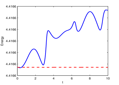
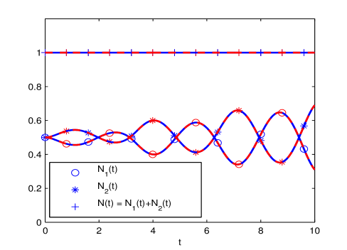
Figure 2: Dynamics of the energy and the total mass for $t=[0,10]$, where the mesh size $h=1/16$ and time step $k=0.0001$. Solid blue line: computed from TSADI method; dash red line: obtained from our method.

In addition, we study the conservation of the energy and total mass. Figure 2 shows the time evolution of the energy and total mass for time $t\in[0,10]$, where the mesh size $h=1/16$ and time step $k=0.0001$. It shows that both the TSADI and our methods conserve the total mass and energy in the discrete level, but our method has a better conservation in energy (c.f. Fig. 2 left).

To further test our method, in Sec. 5.2–5.3 we will apply it to study the dynamical properties of rotating two-component BECs, e.g., dynamics of mass, angular momentum expectation and condensate widths. Our numerical results will be compared with those reported in [44]. In [44], a numerical method was proposed for simulating dynamics of rotating two-component BECs, in which the polar coordinates or cylindrical coordinates were used to resolve the difficulty caused by the angular rotational term and a second- or fourth-order finite difference/element discretion is used in the radial direction. Thus, it has low-order accuracy in the radial direction.

5.2 Dynamics of the mass

We study dynamics of the mass of each component, i.e., $N_{j}(t)=\|\psi_{j}(\cdot,t)\|^{2}$ for $j=1,2$, and also the total mass $N(t)=N_{1}(t)+N_{2}(t)$. In our simulations, we solve two-dimensional CGPEs with the following parameters: $\lambda=1$, $\Omega=0.6$ and two-dimensional harmonic potentials are considered with ${\gamma}_{x,j}={\gamma}_{y,j}=1$ ($j=1,2$). The initial conditions are chosen as

$$\psi_{1}^{0}({\bf x})=\frac{x+iy}{\sqrt{\pi}}\exp\left(-\frac{x^{2}+y^{2}}{2}\right),\qquad\psi_{2}^{0}({\bf x})=0,\qquad\ {\bf x}\in{\mathbb{R}}^{2}.$$

That is, initially all atoms are in the first component. Then we study the dynamics with respect to the following two sets of paramters:

$$\mbox{(i) \ }\left(\begin{array}[]{cc}\beta_{11}&\beta_{12}\\ \beta_{21}&\beta_{22}\end{array}\right)=500\left(\begin{array}[]{cc}1.0&1.0\\ 1.0&1.0\end{array}\right);\qquad\mbox{(ii) \ }\left(\begin{array}[]{cc}\beta_{11}&\beta_{12}\\ \beta_{21}&\beta_{22}\end{array}\right)=500\left(\begin{array}[]{cc}1.0&0.6\\ 0.6&0.8\end{array}\right).$$ (5.13)

This is one example studied in [44]. We remark here that our goal is to test the performance of our method by comparing it with the available method, and thus we use the same example as that in [44] for the purpose of easy comparison.

(a) (b)

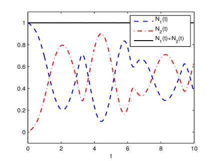
Figure 3: Time evolution of the mass $N_{j}(t)=\|\psi_{j}(\cdot,t)\|^{2}$ ($j=1,2$) and $N(t)=N_{1}(t)+N_{2}(t)$ for two sets of interactions parameters: (a) $\beta_{11}=\beta_{12}=\beta_{22}=500$; (b) $\beta_{11}$ = 500, $\beta_{22}=400$, $\beta_{12}=\beta_{21}=300$.

In our simulations, the computational domain is chosen as ${\mathcal{D}}=[-8,8]^{2}$. We use mesh size $h_{\widetilde{x}}=h_{\widetilde{y}}=\frac{1}{32}$ and time step $\Delta t=0.0001$. Figure 3 shows the time evolution of $N_{1}(t)$, $N_{2}(t)$ and $N(t)$ for time $t\in[0,10]$. From it, we see that when $\beta_{11}=\beta_{12}=\beta_{22}$ (c.f. Fig. 3(a)), the two components exchange their mass periodically with period $T=\pi/\lambda=\pi$. While when $\beta_{11}\neq\beta_{12}\neq\beta_{22}$, $N_{1}(t)$ and $N_{2}(t)$ are not periodical functions (c.f. Fig. 3(b)). In both cases, the total mass $N(t)=N_{1}(t)+N_{2}(t)$ is always conserved. The above observations are consistent with the analytical results reported in [44, 10]. Moreover, our numerical results in Fig. 3 are the same as those obtained in [44] where a numerical method based on Eulerian coordinates was used. However, our extensive simulations show that the computing time taken by our method is much shorter than that by the method in [44], if the same accuracy is required.

5.3 Dynamics of angular momentum expectation and condensate widths

There are two important quantities in describing the dynamics of rotating two-component BECs: angular momentum expectation and condensate widths. In the following, we numerically study their dynamics by applying our method in Sec. 3. For convenience of the readers, we first review the definition of these two quantities; see more information in [8, 44, 43, 10, 13].

The total angular momentum expectation of two-component BECs is defined as

$$\langle L_{z}\rangle(t)=\sum_{j=1}^{2}\int_{\mathbb{R}^{d}}\psi_{j}^{*}({\bf x},t)L_{z}\psi_{j}({\bf x},t)\,d{\bf x},\qquad t\geq 0,$$ (5.14)

and the angular momentum expectation of the $j$th component is

$$\langle L_{z}\rangle_{j}(t)=\frac{1}{N_{j}(t)}\int_{\mathbb{R}^{d}}\psi_{j}^{*}({\bf x},t)L_{z}\psi_{j}({\bf x},t)\,d{\bf x},\qquad t\geq 0,\qquad$$ (5.15)

for $j=1,2$. Usually, the angular momentum expectation can be used to measure the vortex flux. The condensate width of two-component BECs in $\alpha$-direction ($\alpha=x,y$ or $z$) is defined as

$$\sigma_{\alpha}=\sqrt{\delta_{\alpha}(t)}=\sqrt{\delta_{\alpha,1}(t)+\delta_{\alpha,2}(t)},\quad\ t\geq 0,\qquad\alpha=x,\ y\ \mbox{or}\ z,$$ (5.16)

where

$$\delta_{\alpha,j}(t)=\langle\alpha^{2}\rangle_{j}(t)=\int_{{\mathbb{R}}^{d}}\alpha^{2}|\psi_{j}({\bf x},t)|^{2}d{\bf x},\quad\ t\geq 0,\qquad j=1,2.$$ (5.17)

To study the dynamics of angular momentum expectation and condensate widths, we choose the following parameters in the CGPEs (3.1)–(3.2): $d=2$, $\Omega=0.6$, $\lambda=1$ and

$$\left(\begin{array}[]{cc}\beta_{11}&\beta_{12}\\ \beta_{21}&\beta_{22}\end{array}\right)=400\left(\begin{array}[]{cc}1.0&0.97\\ 0.97&0.94\end{array}\right).$$ (5.22)

The initial conditions are taken as

$$\psi_{j}^{0}({\bf x})=\frac{x+iy}{\sqrt{2\pi}}\exp\left(-\frac{x^{2}+y^{2}}{2}\right),\qquad{\bf x}\in{\mathbb{R}}^{2},\quad j=1,2.$$

The computational domain is chosen as ${\mathcal{D}}=[-24,24]^{2}$ with the mesh size $h_{\widetilde{x}}=h_{\widetilde{y}}=\frac{3}{64}$ and time step is $k=0.0001$.

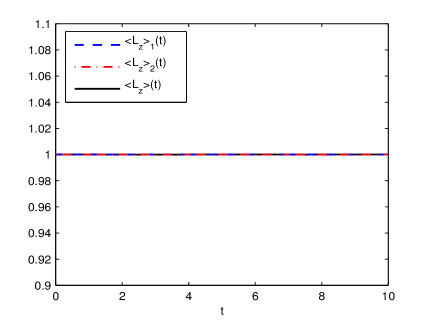
(a) (b)

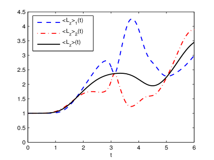
Figure 4: Time evolution of angular momentum expectation $\langle L_{z}\rangle_{j}(t)$ ($j=1,2$) and $\langle L_{z}\rangle$(t) for two sets of trapping frequencies: (a) ${\gamma}_{x,j}={\gamma}_{y,j}=1$ ($j=1,2$); (b) ${\gamma}_{x,1}={\gamma}_{y,1}=1$, ${\gamma}_{x,2}=1.05,{\gamma}_{y,2}=0.9$.

Figure 4 presents the dynamics of angular momentum expectations for two sets of trapping frequencies: (i) ${\gamma}_{x,1}={\gamma}_{y,1}={\gamma}_{x,2}={\gamma}_{y,2}=1$; (ii) ${\gamma}_{x,1}={\gamma}_{y,1}=1$, ${\gamma}_{x,2}=1.05,{\gamma}_{y,2}=0.9$. It shows that the total angular momentum expectation $\langle L_{z}\rangle(t)$ is conserved as long as both external trapping potentials $V_{1}({\bf x})$ and $V_{2}({\bf x})$ in (1.5) are symmetric (c.f. Fig. 4(a)). While when $\lambda\neq 0$, if at least one of the external potentials is asymmetric, none of $\langle L_{z}\rangle_{1}(t)$, $\langle L_{z}\rangle_{2}(t)$ and $\langle L_{z}\rangle(t)$ is conserved (c.f. Fig. 4(b)). In addition, the results in Fig. 4 are the same as those reported in [44] but the computing time used by our method is much less.

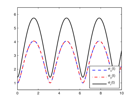
(a) (b)

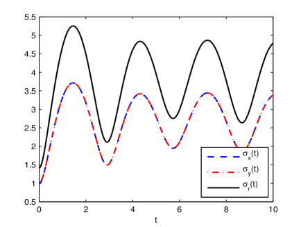
Figure 5: Time evolution of condensate widths $\sigma_{x}(t)$, $\sigma_{y}(t)$ and $\sigma_{r}(t)$ for two sets of trapping frequencies: (a) ${\gamma}_{x,j}={\gamma}_{y,j}=1$ ($j=1,2$); (b) ${\gamma}_{x,1}={\gamma}_{y,1}=1$, ${\gamma}_{x,2}={\gamma}_{y,2}=1.2$.

Figure 5 shows the dynamics of condensate widths for $\sigma_{x}(t)$, $\sigma_{y}(t)$ and $\sigma_{r}(t):=\sqrt{\sigma_{x}^{2}(t)+\sigma^{2}_{y}(t)}$ for two sets of trapping frequencies: (i) ${\gamma}_{x,1}={\gamma}_{y,1}={\gamma}_{x,2}={\gamma}_{y,2}:=\gamma=1$; (ii) ${\gamma}_{x,1}={\gamma}_{y,1}=1$, ${\gamma}_{x,2}={\gamma}_{y,2}=1.2$. From it, we see that when the two components have the same external trapping potentials, the condensate widths $\sigma_{x}(t)$, $\sigma_{y}(t)$ and $\sigma_{r}(t)$ are periodic functions with period $T=\pi/\gamma=\pi$ (c.f. Fig. 5(a)). If the potential $V_{1}({\bf x})\neq V_{2}({\bf x})$ in (1.5), the condensate widths are not periodic functions. The above results are consistent with those in [44].

5.4 Dynamics of vortex lattices

In this section, we apply our method to study the dynamics of vortex lattices in rotating two-component BECs. The initial data are taken as the stationary vortex lattices, which are computed by choosing $\Omega=0.9$, $\lambda=0$, ${\gamma}_{x,j}={\gamma}_{y,j}=1$ ($j=1,2$) and

$$\left(\begin{array}[]{c c}\beta_{11}&\beta_{12}\\ \beta_{21}&\beta_{22}\end{array}\right)=500\left(\begin{array}[]{cc}1.0&-0.25\\ -0.25&1.0\end{array}\right).$$

Due to the attractive interaction between two components, i.e., $\beta_{12}=\beta_{21}<0$, initially the stationary vortex lattices are exactly the same. Then at time $t=0$,

1. Case (i). Change the symmetric external potentials to asymmetric by setting $\gamma_{x,1}=\gamma_{y,2}=1.05$ and $\gamma_{x,2}=\gamma_{y,1}=0.95$;

2. Case (ii). Turn on the external driving field by setting $\lambda=1$.

Then we study the dynamics of vortex lattices. The computational domain is chosen as ${\mathcal{D}}=[-24,24]^{2}$ with $h_{\widetilde{x}}=h_{\widetilde{y}}=\frac{3}{32}$ and the time step $k=0.0001$.

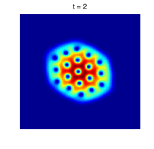
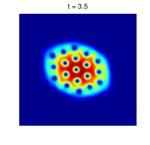
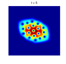
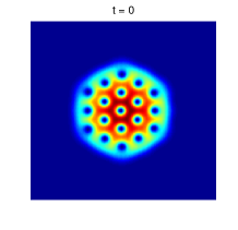
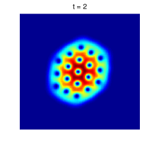
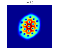
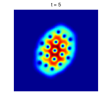
Figure 6: Contour plots of the density $|\psi_{1}|^{2}$ (top row) and $|\psi_{2}|^{2}$ (bottom row) at different time for Case (i). Displayed domain $(x,y)\in[-10,10]^{2}$.

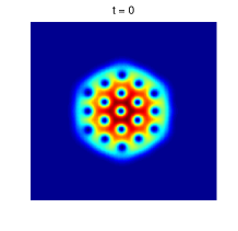
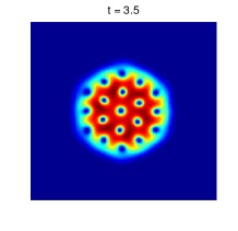
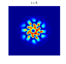
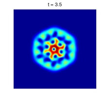
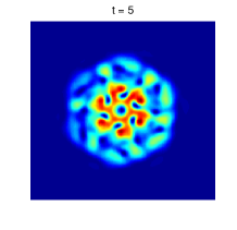
Figure 7: Contour plots of the density $|\psi_{1}|^{2}$ (top row) and $|\psi_{2}|^{2}$ (bottom row) at different time for Case (ii). Displayed domain $(x,y)\in[-10,10]^{2}$.

Figures 6–7 show the contour plots of the density $|\psi_{1}|^{2}$ and $|\psi_{2}|^{2}$ at different time $t$ in Case (i) and (ii), respectively, where the displayed domain is $(x,y)\in[-10,10]^{2}$. At $t=0$, the vortex lattices are identical and there are 19 vortices in each lattice. In Case (i), the lattices rotate periodically due to the anisotropy of the external potentials and the number of vortices is conserved during the dynamics (c.f. Fig. 6). While in Fig. 7, we see that the external driving field eventually destroys the pattern of vortex lattices.

6 Summary

We proposed an efficient numerical method to solve the coupled Gross–Pitaevskii equations (CGPEs) with both angular momentum rotation term and external driving field term, which well describes the dynamics of rotating two-component Bose–Einstein condensations (BECs) with an internal Josephson junction. We introduced a rotating Lagrangian coordinate transformation and then eliminated the angular momentum rotation term in the CGPEs. Under the new coordinates, we proposed a time-splitting sine pseudospectral method to simulate the dynamics of rotating two-component BECs. To efficiently treat the external driving field term, we applied a linear transformation so that it does not cause any extra computational complexity. Compared to the methods in literature has higher order spatial accuracy but requires less memory cost and computational cost. It can be easily implemented in practice. We then numerically examined the conservation of the angular momentum expectation and studied the dynamics of condensate widths and center of mass for different angular velocities. In addition, the dynamics of vortex lattice in rotating two-component BECs were investigated. Numerical studies showed that our method is very effective.

Acknowledgements    Q. Tang and Y. Zhang would like to express their sincere thanks to Prof. Weizhu Bao for the fruitful discussion on the project. This work was partially supported by the Singapore A*STAR SERC Grant No. 1224504056 (Q. Tang) and by the Simons Foundation Award No. 210138 (Y. Zhang).

References

References

- [1] J.R. Abo-Shaeer, C. Raman, J.M. Vogels and W. Ketterle, Observation of vortex lattices in Bose–Einstein condensates, Science, 292 (2001), pp. 210–236.
- [2] M.H. Anderson, J.R. Ensher, M.R. Matthews, C.E. Wieman and E.A. Cornell, Observation of Bose–Einstein condensation in a dilute atomic vapor, Science, 269 (1995), pp. 198–201.
- [3] X. Antoine, C. Besse and P. Klein, Numerical solution of time-dependent nonlinear Schrödinger equations using domain truncation techniques coupled with relaxation scheme, Laser Physics, 21 (2011), pp. 1–12.
- [4] P. Antonelli, D. Marahrens and C. Sparber, On the Cauchy problem for nonlinear Schrödinger equations with rotation, Disc. Contin. Dyn. Syst. A, 32 (2012), pp. 703–715.
- [5] W. Bao, Ground states and dynamics of multicomponent Bose–Einstein condensates, Multiscale Model. Simul., 2 (2004), pp. 210–236.
- [6] W. Bao, Q. Tang and Z. Xu, Numerical methods and comparison for computing dark and bright solitons in the nonlinear Schrödinger equation, J. Comput. Phys., 235 (2013), pp. 423–445.
- [7] W. Bao and Y. Zhang, Dynamics of the ground state and central vortex state in Bose–Einstein condensation, Math. Mod. Meth. Appl. Sci., 15 (2005), pp. 1863-1896.
- [8] W. Bao, Q. Du and Y. Zhang, Dynamics of rotating Bose–Einstein condensates and its efficient and accurate numerical computation, SIAM J. Appl. Math., 66 (2006), pp. 758–786.
- [9] W. Bao and H. Wang, An efficient and spectrally accurate numerical method for computing dynamics of rotating Bose–Einstein condensates, J. Comput. Phys., 217 (2006), pp. 612–626.
- [10] W. Bao, Analysis and efficient computation for the dynamics of two-component Bose–Einstein condensate, Comtemporary Mathematics, AMS, 473 (2008), pp. 1–26.
- [11] W. Bao, H. Li and J. Shen, A generalized Laguerre–Fourier–Hermite pseudospectral method for computing the dynamics of rotating Bose–Einstein condensates, SIAM J. Sci. Comput., 31 (2009), pp. 3685–3711.
- [12] W. Bao and Y. Cai, Ground states of two-component Bose–Einstein condensates with an internal atomic Josephson junction, East Asian J. Appl. Math., 1 (2011), pp. 49-81.
- [13] W. Bao, D. Marahens, Q. Tang and Y. Zhang, A simple and efficient numerical method for computing the dynamics of rotating Bose–Einstein condensates via a rotating Lagrangian coordinate, preprint, (2013).
- [14] J.P. Boyd, A fast algorithm for Chebyshev, Fourier, and since interpolation onto an irregular grid, J. Comput. Phys., 103 (1992), pp. 243–247.
- [15] C.C. Bradley, C.A. Sackett, J.J. Tollett and R.G. Hulet, Evidence of Bose–Einstein condensation in an atomic gas with attractive interaction, Phys. Rev. Lett., 75 (1995), pp. 1687–1690.
- [16] S. Chang, C. Lin, T. Lin and W. Lin, Segregated nodal domains of two dimensional multispecies Bose–Einstein condensates, Physica D, 196 (2004), pp. 341–361.
- [17] G.-H. Chen and Y.-S. Wu, Quantum phase transition in a multi-component Bose–Einstein condensate in optical lattices, Phys. Rev. A, 67 (2003), article 013606.
- [18] S.T. Chui, V.N. Ryzhov and E.E. Tareyeva, Phase separation and vortex states in the binary mixture of Bose–Einstein condensates, J. Exper. Thect. Phys., 91 (2000), pp. 1183–1189.
- [19] I. Corro, R.G. Scott and A.M. Martin, Dynamics of two-component Bose–Einstein condensates in rotating traps, Phys. Rev. A, 80 (2009), article 033609.
- [20] K.B. Davis, M.O. Mewes, M.R. Andrews, N.J. van Druten, D.S. Durfee, D.M. Kurn and W. Ketterle, Bose–Einstein condensation in a gas of sodium atoms, Phys. Rev. Lett., 75 (1995), pp. 3969–3973.
- [21] A.L. Fetter, Rotating trapped Bose–Einstein condensates, Rev. Mod. Phys., 81 (2009), pp. 647–691.
- [22] J.J. García-Ripoll, V.M. Pérez–García and V. Vekslerchik, Construction of exact solution by spatial translations in inhomogeneous nonlinear Schrödinger equations, Phys. Rev. E, 64 (2001), article 056602.
- [23] R. Glowinski and P. Le Tallec, Augmented Lagrangian and operator splitting methods in nonlinear mechanics, SIAM Stud. Appl. Math., 9 (1989) SIAM, Philadelphia.
- [24] D.S. Hall, M.R. Matthews, J.R. Ensher, C.E. Wieman and E.A. Cornell, Dynamics of component separation in a binary mixture of Bose–Einstein condensates, Phys. Rev. Lett., 81 (1998), pp. 1539–1542.
- [25] T.-L. Ho and V.B. Shenoy, Binary mixtures of Bose condensates of alkali atoms, Phys. Rev. Lett., 77 (1996), pp. 3276–3279.
- [26] C.-H. Hsueh, T.-L. Horng, S.-C.Gou and W.C. Wu, Equilibrium vortex formation in ultrarapidly rotating two-component Bose–Einstein condensates, Phy. Rev. A, 84 (2011), article 023610.
- [27] D.M. Jezek, P. Capuzzi and H.M. Cataldo, Structure of vortices in two-component Bose–Einstein condensates, Phys. Rev. A, 64 (2001), article 023605.
- [28] J. Jin, S. Zhang, W. Han and Z. Wei, The ground states and spin textures of rotating two-component Bose–Einstein condensates in an annular trap, J. Phys. B: At. Mol. Opt. Phys., 46 (2013), article 075302.
- [29] K. Kasamatsu, M. Tsubota and M. Ueda, Spin-textures in rotating two-component Bose–Einstein condensates, Phys. Rev. A, 71 (2004), article 043611.
- [30] K. Kasamatsu, M. Tsubota and M. Ueda, Vortex phase diagram in rotating two-component Bose–Einstein condensates, Phys. Rev. Lett., 91 (2003), article 150406.
- [31] K. Kasamatsu, M. Tsubota and M. Ueda, Vortices in multicomponent Bose–Einstein condensates, Inter. J. Modern Phys. B, 19 (2005), pp. 1835–1904.
- [32] D. Kobyakov, V. Bychkov, E. Lundh, A. Bezett, V. Akkerman and M. Marklund, Interface dynamics of a two-component Bose–Einstein condensate driven by an external force, Phys. Rev. A, 83 (2011), article 043623.
- [33] E.H. Lieb and R. Seiringer, Derivation of the Gross–Pitaevskii equation for rotating Bose gases, Comm. Math. Phys., 264 (2006), pp. 505–537.
- [34] Z. Liu, Rotating multicomponent Bose–Einstein condensates, Nonl. Differ. Equ. Appl., 19 (2012), pp. 49–65.
- [35] T. Lin and J. Wei, Ground states of coupled nonlinear Schrödinger equations in , , Comm. Math. Phys., 255 (2005), pp. 629–653.
- [36] M.R. Matthews, B.P. Anderson, P.C. Haljan, D.S. Hall, C.E. Wiemann and E.A. Cornell, Vortices in a Bose–Einstein condensate, Phys. Rev. Lett., 83 (1999), pp. 2498–2501.
- [37] K.W. Madison, F. Chevy, W. Wohlleben and J. Dalibard, Vortex formation in a stirred Bose–Einstein condensate, Phys. Rev. Lett., 84 (2000), pp. 806–809.
- [38] K.W. Madison, F. Chevy, V. Bretin and J. Dalibard, Stationary states of a rotating Bose–Einstein condensates: Routes to vortex nucleation, Phys. Rev. Lett., 86 (2001), pp. 4443–4446.
- [39] C.J. Myatt, E.A. Burt, R.W. Ghrist, E.A. Cornell and G. E. Wieman, Production of two overlapping Bose–Einstein condensates by sympathetic cooling, Phys. Rev. Lett., 78 (1997), pp. 586–589.
- [40] M. Sepúlveda and O. Vera, Numerical methods for a coupled nonlinear Schrödinger system, Bol. Soc. Esp. Mat. Apl., 43 (2008), pp. 95–102.
- [41] J. Shen, T. Tang and L. Wang, Spectral Methods: Algorithms, Analysis and Applications, Springer, 2011.
- [42] G. Strang, On the construction and comparison of difference schemes, SIAM J. Numer. Anal., 5 (1968), pp. 505-517.
- [43] H. Wang, A time-splitting spectral method for coupled Gross–Pitaevskii equations with applications to rotating Bose–Einstein condensates, J. Comput. Appl. Math., 205 (2007), pp. 88–104.
- [44] Y. Zhang, W. Bao and H. Li, Dynamics of rotating two-component Bose–Einstein condensates and its efficient computation, Physica D, 234 (2007), pp. 49–69.
- [45] D. Jaksch, S.A. Gardiner, K. Schulze, J.I. Cirac and P. Zoller, Uniting Bose–Einstein condensates in optical resonators, Phys. Rev. Lett., 86 (2001), pp. 4733–4736.