Real-space density functional theory on graphical processing units: computational approach and comparison to Gaussian basis set methods

Abstract

We discuss the application of graphical processing units (GPUs) to accelerate real-space density functional theory (DFT) calculations. To make our implementation efficient, we have developed a scheme to expose the data parallelism available in the DFT approach; this is applied to the different procedures required for a real-space DFT calculation. We present results for current-generation GPUs from AMD and Nvidia, which show that our scheme, implemented in the free code octopus, can reach a sustained performance of up to 90 GFlops for a single GPU, representing a significant speed-up when compared to the CPU version of the code. Moreover, for some systems our implementation can outperform a GPU Gaussian basis set code, showing that the real-space approach is a competitive alternative for DFT simulations on GPUs.

I Introduction

For many years, the constant reduction in the size of the transistors, as described by Moore’s law Moore (1965), has been translated into an increment of the processing capacity of central processing units (CPUs). However, due to the limitations in efficiency and power consumption related to the breakdown of Dennard scaling Dennard et al. (1974); *Bohr2009, CPU designers moved towards parallel processing to profit from the increasing number of transistors. This trend towards parallelism can be seen in current CPUs, that have multiple cores, with each core capable of executing multiple threads and containing vectorial processing units that operate simultaneously on several sets of values.

Simultaneously, a more parallel kind of processor appeared: the graphical processing unit (GPU). Originally designed for real-time rendering of images, a computationally intensive and highly-parallel task, modern GPUs are also suitable for general purpose computing, in particular for high-performance numerical simulations. They typically have thousands of execution units, that give them approximately one order of magnitude higher processing power than a CPU. This difference is explained by different design strategies: while a single instruction may be executed faster on a CPUs, GPUs can execute thousands of them in parallel.

In the last years there has been a considerable interest in applying GPUs to computational science. While in some areas of atomistic simulations GPUs are becoming a standard tool Harju et al. (2013), in the electronic structure domain, and in particular in density functional theory (DFT) Hohenberg and Kohn (1964); *Kohn1965, the adoption of GPUs has been slower. The first full electronic-structure implementation on GPUs was terachem, presented by Ufimtsev and Martínez in 2008 Ufimtsev and Martínez (2008a). Currently, several electronic structure codes have also incorporated some degree of GPU acceleration Yasuda (2008); Vogt et al. (2008); Genovese et al. (2009); Watson et al. (2010); Tomono et al. (2010); Andrade and Genovese (2012); Andrade et al. (2012a); Maintz et al. (2011); DePrince and Hammond (2011); Spiga and Girotto (2012); Maia et al. (2012); Hacene et al. (2012); Esler et al. (2012); Hakala et al. (2013); Jia et al. (2013a); *Jia2013b; Hutter et al. (2013).

Still, how to get the most out of a GPU for modeling electronic systems is an active area of research Spiga and Girotto (2012); Bhaskaran-Nair et al. (2013); Titov et al. (2013), as simulation approaches that are efficient on a CPU might not be as efficient on a GPU. These approaches can be improved or replaced by other methods that are better suited to massively parallel architectures. In this respect, the large diversity of methods used for electronic structure methods by chemists and physicist, offers an interesting starting point to explore the application of GPUs to the simulation of electronic systems.

In this work we focus on one particular approach for electronic structure, real-space DFT, and how it can be adapted to GPUs. While not as widely used as basis-set methods, the real-space grid discretization is a popular alternative for DFT simulations Becke (1989); Chelikowsky et al. (1994); Briggs et al. (1995); Fattebert and Bernholc (2000); Fattebert and Nardelli (2003); Beck (2000); Marques et al. (2003); Torsti et al. (2003); Hirose (2005); Mortensen et al. (2005); Kronik et al. (2006); Yabana et al. (2006); Hernández et al. (2007); Iwata et al. (2010). Its main features are the flexibility to model different types of electronic systems, the systematic control of the discretization error, and its potential for parallelization in distributed memory systems with thousands of processors Andrade et al. (2012a); Bernholc et al. (2008); Enkovaara et al. (2010); Hasegawa et al. (2011).

The development of an efficient GPU implementation does not only involve rewriting and optimizing low-level routines for the GPU. For complex scientific software, choosing an appropriate design strategy for the entirety of the code can be fundamental for optimal GPU performance. This work is mainly focused on this issue: we have developed a scheme to apply DFT efficiently on GPUs by exposing the available parallelism to the low-level routines.

Our approach was developed for the implementation of GPU support in the octopus code Marques et al. (2003); Castro et al. (2006); Andrade et al. (2012a) and is freely available under an open source license oct . Octopus is used by several research groups for theoretical development Burnus et al. (2005); Botti et al. (2008); Andrade et al. (2009); Räsänen et al. (2010); Helbig et al. (2011); De Giovannini et al. (2012); Elliott et al. (2012); Andrade et al. (2012b) and applications in different fields of chemistry and physics Wasserman et al. (2008); Malloci, G. et al. (2008); Botti et al. (2009); Vila et al. (2010); Zhang et al. (2011); Bonaca and Bilalbegović (2011); Avendaño Franco et al. (2012); Castro (2013); Andrea Rozzi et al. (2013); Räsänen and Heller (2013). In this article, we describe in detail our general strategy and its application to the different procedures required for real-space DFT, extending previous results for real-time time-dependent DFT Andrade and Genovese (2012); Andrade et al. (2012a). Our GPU implementation is based on OpenCL Munshi (2009), a standard and portable framework for writing code for parallel processors, so it can run on GPUs, CPUs, and other processing devices, from different vendors.

In order to assess the efficiency of our implementation, we perform a series of tests involving top-end GPUs from Nvidia and AMD, and a set of molecular systems of different sizes. We provide different indicators that illustrate the performance of our implementation: numerical throughput (number of floating point operations executed per unit of time), total calculation times, and comparisons with the CPU version of the code and a different GPU-DFT implementation. These results show that real-space DFT is an interesting and competitive approach for GPU-accelerated electronic structure calculations.

II Real-space density functional theory

In the Kohn-Sham (KS) formulation of DFT, the electronic density of an interacting electronic system, $n({\bm{r}})$, is generated by a set of single-particle orbitals, or states, $\varphi_{k}({\bm{r}})$. These orbitals are generated by the KS equations Hohenberg and Kohn (1964); *Kohn1965

$$H[n]\varphi_{k}({\bm{r}}) =\epsilon_{k}\,\varphi_{k}({\bm{r}})$$ (1a)

$$n({\bm{r}}) =\sum_{k=1}^{N}\varphi_{k}^{*}({\bm{r}})\varphi_{k}({\bm{r}})\ ,$$ (1b)

where the $H$ operator is the KS effective single-particle Hamiltonian, (atomic units are used throughout)

$$H[n]=-\frac{1}{2}\nabla^{2}+v_{\mathrm{ext}}({\bm{r}})+v_{\mathrm{hxc}}[n]({\bm{r}},t)\ .$$ (2)

The external potential $V_{\mathrm{ext}}$ contains the nuclear potential and other external fields that may be present, $V_{\mathrm{hxc}}$ represents the electron-electron interaction and is usually divided in the Hartree term, that contains the classical electrostatic interaction between electrons, and the exchange and correlation (XC) potential.

To solve the KS equations numerically, the orbitals, the density, and other fields need to be represented as a finite set of numbers. The selection of the discretization scheme is probably the most important aspect in the numerical solution of the electronic structure problem. Traditionally, a basis set expansion is used: atomic orbitals for molecules, and plane waves for crystalline systems. In the real-space approach, instead of a basis, fields are discretized in a grid. This provides a simple and flexible scheme that is suitable to model both finite and periodic systems Natan et al. (2008). The electron ion interaction is modeled by the pseudo-potential approximation, or the projector-augmented-wave method Mortensen et al. (2005), that remove the problem of representing the hard Coulomb potential, so uniform grids can be used.

One of the main advantages of the real-space grid approach is that the discretization error can be controlled systematically by reducing the spacing and increasing the size of the box. Of course, this increases the number of points and, proportionally, the time and memory cost of the calculation. To keep the number of grid points to a minimum, our implementation uses arbitrarily-shaped grids. This choice makes the code more complex but allows for an important reduction in grid size compared with a simpler cubic grid. For molecular systems we use a uniform grid whose shape is given by the union of spheres around each atom, as shown in Fig. 1. This strategy avoids placing points in regions where the value of the density is not significant for the desired accuracy.

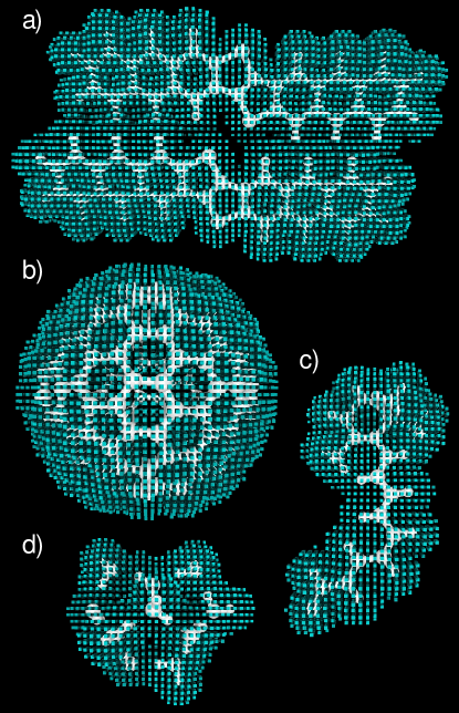
Figure 1: Examples of real-space grids adapted to the shape of different molecular systems: a) DAT-thiophane dimer b) C₁₈₀ fullerene c) cis-retinal d) water cluster. The (cyan) cubes mark the position of the grid points. For visualization purposes, we represent smaller and coarser grids than the ones used for actual calculations.

III Numerical solution of real-space density functional theory

We now describe the numerical procedure to solve the KS equations in real-space. As it is standard in Hartree-Fock (HF) and DFT, in order to account for the nonlinearity introduced by the density dependence in eq. (1) a self-consistent field (SCF) iterative scheme is used. A new set of orbitals and density are generated each SCF iteration; this involves several numerical procedures, that are shown in Fig. 2.

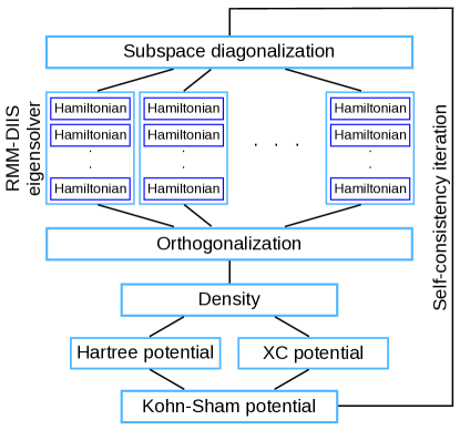
Figure 2: Schematic of a density functional theory calculation in real-space using a self-consistency scheme and the residual minimization-direct inversion in the iterative subspace (RMM-DIIS) eigensolver. The boxes represent the different numerical procedures that need to be performed.

Every SCF step we need to find the lower eigenvectors and eigenvalues of the KS Hamiltonian for a fixed density. In real-space, the discretization of the KS Hamiltonian, eq. (2), is done using a high-order finite differences representation Chelikowsky et al. (1994). As this results in a sparse operator, the diagonalization is done using iterative methods that do not require the Hamiltonian matrix to be built explicitly, only to be applied as an operator. In this work, we use the efficient residual minimization-direct inversion in the iterative subspace (RMM-DIIS) eigensolver Wood and Zunger (1985); Kresse and Furthmüller (1996) (not to be confused with the DIIS SCF scheme Pulay (1980)). To precondition the eigensolver, we use the filter operator proposed by Saad et al. Saad et al. (1996).

In practice, it is not worth it to find a converged solution of the eigenvalue problem at each SCF iteration: instead we do a fixed number of eigensolver iterations per step. In this manner, the eigenproblem convergence is achieved towards the end of the SCF cycle.

The RMM-DIIS scheme requires the application of the KS Hamiltonian and two additional procedures that act over the whole set of orbitals: orthogonalization and subspace diagonalization. Given a set of orbitals, the orthogonalization procedure performs a linear transformation that generates a new orthogonal set. Similarly, subspace diagonalization is an effective method to remove contamination between orbitals. It calculates the representation of the KS Hamiltoninan in the subspace spanned by a set of orbitals, and generates a new set where the subspace Hamiltonian is diagonal.

After the eigensolver steps and the posterior orthogonalization, a new set of orbitals and a new density are obtained; this density is mixed with the densities from previous steps to generate a new guess density according to the Broyden scheme Broyden (1965); Srivastava (1984).

From the new guess density, the new KS effective potential is calculated. Numerically, the most expensive part of this step is obtaining the Hartree potential, $V_{\mathrm{H}}$, that requires the solution of the Poisson equation

$$\nabla^{2}V_{\mathrm{H}}({\bm{r}})=-4\pi\,n({\bm{r}})\ .$$ (3)

In our implementation, we use a Poisson solver based on fast Fourier transforms. The XC potential, $v_{\mathrm{xc}}$, also needs to be recalculated. This is approximated by a local or semi-local expression that is evaluated directly on the grid.

IV General GPU optimization strategy

In this section we discuss the general scheme that we have developed to solve efficiently the real-space DFT equation on GPUs. This strategy was designed taking into account the strengths and weaknesses of the current generation of GPUs, but is also effective for CPUs with vectorial floating point units.

For optimum efficiency, GPUs need to operate simultaneously over large amounts of data, so that the numerous independent operations fill the execution units and hide operation and memory latency (the time it takes the result of an instruction to be available to other instructions). A way to fulfill this requirement is to expose data-parallelism to the low-level routines. For example, if the same operation needs to be performed over certain data objects, the routines should receive as an argument a group of those objects, instead of operating over one object per call.

In order to expose parallelism in the DFT case, our GPU optimization strategy is based on the concept of blocks of KS orbitals. Instead of acting over a single KS orbital at a time, performance critical routines receive a group of orbitals as argument. By operating simultaneously over several orbitals, the amount of parallelism exposed to the processor is increased considerably. In Fig. 3 we show a scheme of how this concept works.

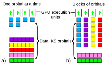
Figure 3: Scheme illustrating the blocks of orbitals strategy for DFT on GPUs. a) Operating on a single orbital might not provide enough parallelism for the GPU to perform efficiently. b) By operating simultaneously over several orbitals there is a larger degree of data parallelism and there is less divergence among GPU threads.

The blocks-of-orbitals strategy has an additional advantage: in a GPU, threads are divided in groups of 32 (Nvidia) or 64 (AMD), called warps or wavefronts; for efficient execution all threads in a warp must execute exactly the same instruction sequence. Since the same operation has to be performed over each orbital, we can assign operations corresponding to different orbitals to different threads in a warp. This ensures that the execution within each warp is regular, without divergences in the instruction sequence. In a CPU, vectorial floating point units play a similar role as warps.

A possible drawback of the block-of-orbitals approach is that memory access issues might appear, as working with larger amount of data can saturate caches and reduce their ability to speed-up memory access. This is especially true for CPUs, which rely more on caches than GPUs. Larger blocks can also increase the amount of memory required for temporary data. So using blocks that are too large might be detrimental for performance.

In our implementation the number of orbitals in a block, or block-size, is variable and controlled at execution time. Ideally the block-size should be an integer multiple of the warp-size. This might not be possible if not enough orbitals are available, in such a case the block-size should be a divisor of the warp size. Following these considerations we restrict our block-size to be a small power of two .

The way blocks of orbitals are stored in memory is also fundamental for optimal performance. A natural scheme would be to store the coefficients for each orbital (Fig. 4a) contiguously in memory, so that each orbital in a block can be easily accessed. However, memory access is usually more efficient when threads access adjacent memory locations as loads or stores go to the same cache-lines. Since in our approach consecutive threads are assigned to different orbitals, we order blocks by the orbital index first and then by the discretized ${\bm{r}}$-index, ensuring that adjacent threads will access adjacent memory locations (Fig. 4b).

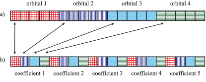
Figure 4: Example of memory layout for a block of 4 orbitals with 5 coefficients each: (a) Standard memory layout where each orbital is contiguous in memory. (b) Optimal memory layout where all the coefficients in a block are contiguous. The arrows indicate the relation of the position of the first coefficient in both schemes.

In the following sections, we show how these general strategies are applied to the different numerical procedures that were introduced in section III. For each operation we show the numerical performance that our implementation obtains for a test system, $\beta$-cyclodextrin, on an Intel Core i7 3820 CPU and two GPUs, an AMD Radeon HD 7970 and a Nvidia Tesla K20 (shown in Fig. 5). Details about the platforms and the calculations can be found in section XII.

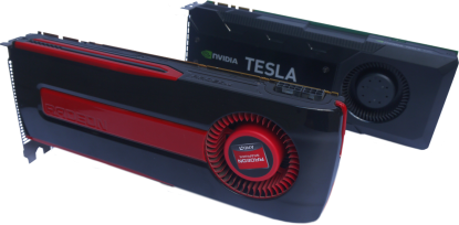
Figure 5: AMD Radeon HD 7970 and a Nvidia Tesla K20 GPU cards used for the numerical tests.

V Kohn-Sham Hamiltonian

The application of the KS Hamiltonian, eq. (2), is the basic operation of the real-space DFT approach, as such, it is the first target for efficient GPU execution. Moreover, the KS Hamiltonian application is also used in other DFT-based simulations like on-the-fly molecular dynamics Tuckerman and Parrinello (1994); *Alonso2008, and response calculations in time Yabana and Bertsch (1996); *Castro2004 and frequency domains Baroni et al. (2001); *Andrade2007.

As a matrix, the real-space KS Hamiltonian operator is sparse, with a number of coefficients that is proportional to the number of grid points. While the matrix could be stored in a sparse form, it is not convenient to do so. It is more efficient to use it in operator form, with three different terms that are applied independently: the kinetic energy operator, the local potential, and the non-local potential.

V.1 Kinetic energy operator

In real-space the kinetic-energy operator corresponds to the Laplacian differential operator. While in a basis-set approach this term is calculated exactly, in real-space the Laplacian is approximated using high-order finite-differences Chelikowsky et al. (1994). Numerically, this is a stencil calculation, where the value at each point is calculated as a linear combination of the neighboring-point values. The stencil represents the grid points used in the calculation of the differential operator, see Fig. 6 for an example. In the simulations presented in this paper we use a fourth-order approximation that in 3D results in a stencil size of 25.

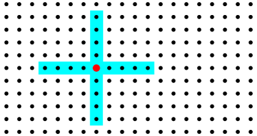
Figure 6: Example of a stencil for the fourth-order Laplacian in a 2D grid. The values from points in the colored region are used to calculate the Laplacian in the central (red) point.

Since stencil calculations are common in scientific and engineering applications, their optimization in CPU and GPU architectures has received considerable interest Peng et al. (2009); Datta et al. (2009); Dursun et al. (2009); Treibig et al. (2011); de la Cruz and Araya-Polo (2011); Henretty et al. (2011); Holewinski et al. (2012). In our approach the stencil is applied over several orbitals at once, avoiding some of the performance issues that appear in the application of a stencil to a single dataset, in particular with respect to vectorization Henretty et al. (2011).

On the GPU, to perform the application of the Laplacian over a block of orbitals the threads are arranged in a two-dimensional grid: the first dimension corresponds to the orbital index and the second to the point index. The first task of each group of threads is to find the location of the neighboring points in the input array. Since the grid has an arbitrary shape, this location cannot be easily calculated and we need to use a table of neighbors . Once the neighbor addresses are obtained, each thread iterates over the stencil position loading the neighbor value, multiplying it by the corresponding weight and accumulating the result.

Memory access is usually the limiting factor for the performance of the finite-difference operators Datta et al. (2009), as for each point we need to iterate over the stencil loading values that are only used for one multiplication and one addition. As the values of the neighbors are scattered, memory access is not regular. This part of the problem is addressed by using blocks of orbitals: since the Laplacian is calculated over a group of orbitals at a time, for each point of the stencil we load several values, one per orbital in the block, that are contiguous in memory. This makes memory access more regular and hence more efficient for both GPUs and CPUs.

Still, a potential problem with memory access persists. As each input value of the stencil has to be loaded several times, ideally it should be loaded from main memory once and kept in cache for subsequent uses. Unfortunately, as the stencil operation has poor memory locality, this is not always the case.

We devised an approach to improve cache utilization by controlling how grid points are ordered in memory, i.e., how the three-dimensional grid is mapped to a linear array. The standard approach is to use a row-major or column-major order which leads to some neighboring points being allocated in distant memory locations. Our approach is to enumerate the grid points based on a sequence of small parallelepipedic grids, as shown in the example of Fig. 7. This approach permits close spatial regions to be stored closer in memory, improving memory locality for the Laplacian operator. The effect of this optimization can be seen in Fig. 8, where we compare the throughput of the Laplacian operator, as a function of the block-size, for the optimized grid order with respect to the standard one. For the CPU with the standard ordering of points, there is only a small gain performance from using blocks of orbitals, while by optimizing the grid order, the parallelism exposed by a larger block size allows a considerable performance gain. For the GPU the effect of the optimization is less dramatic but still significant.

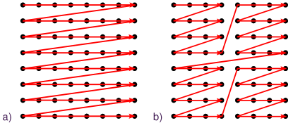
Figure 7: Examples of different grid orders in 2D: (a) standard order (b) grid ordered by small parallelepipedic blocks.

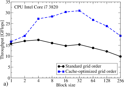
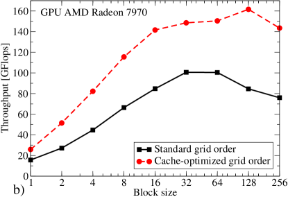
Figure 8: Effect of the optimization of the grid mapping for data locality in the numerical throughput of the Laplacian operator as a function of the size of the orbitals block. Spherical grid with  500k points. a) computations with an Intel Core i7 3820 (8 threads). b) computations with a AMD Radeon 7970.

An area for further improvement, is that the optimal size of the parallelepipedic subgrids depends on the processor and the shape and size of the grid, which change for each molecule. Since it is not practical to optimize these parameters for each case, we use a fixed set that does not always yield the best possible performance. This can be seen in Fig. 9, where we show a comparison of the numerical throughput of the GPU and CPU implementations of the Laplacian operator for a $\beta$-cyclodextrin molecule: the performance obtained is not as high as in Fig. 8. We plan to study the applicability of more sophisticated space-filling curves Peano (1890); *Sagan1994; *Gunther2006 to address this issue.

It is clear from Fig. 9 that for all processors, the use of blocks of KS states represents a significant numerical performance gain with respect to working with one state at a time. This is particularly important for GPUs, where performance with a single state is similar to the CPU, but it is more than five times larger with blocks of size 32 or 64.

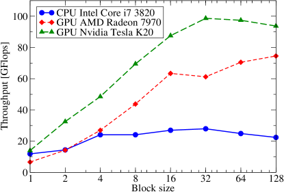
Figure 9: Numerical throughput of the calculation of the finite-difference fourth-order Laplacian as a function of the size of the block of orbitals (block-size) for different processors. Calculation for $\beta$-cyclodextrin with 256 orbitals and 260k grid points.

V.2 Local potential

The second term of the Hamiltonian is the local potential, that includes contributions from the external potential, including the local parts of the pseudo-potentials, the Hartree, exchange, and correlation potentials. All these terms are summed into a single potential, so we only need to multiply each orbitals by this potential and store the result.

Since there are only two arithmetic operations per element, the application of the local potential is heavily limited by memory access. Using blocks of orbitals has two beneficial effects: the larger number of simultaneous operations can hide the memory latency, and the values of the potential are reused, reducing the number of memory accesses. In Fig. 10, we compare the numerical performance of the application of the local potential for different processors. As expected, the GPU has a considerable performance advantage caused by the higher memory bandwidth. Still, the numerical throughput is significantly below the values we obtain for other parts of the calculation.

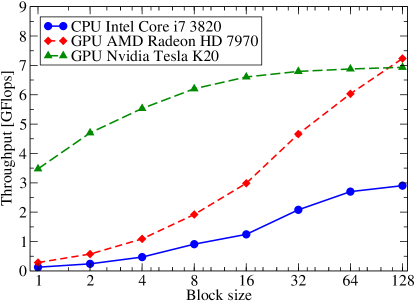
Figure 10: Numerical throughput of the application of the local potential as a function of size of the block of orbitals (block-size) for different processors. Calculation for $\beta$-cyclodextrin with 256 orbitals and 260k grid points.

V.3 Non-local potential

The final term required for the application of the Hamiltonian is the non-local potential that comes from the norm-conserving pseudo-potentials Kleinman and Bylander (1982); *Troullier1991. The non-locality comes from the fact that each angular momentum component of the orbital sees a different potential. In practice, we calculate

$$V_{\mathrm{nl}}\varphi_{k}({\bm{r}})=\sum_{A}\sum_{lm}\gamma^{A}_{lm}({\bm{r}}-{\bm{R}})\int_{r^{\prime}<r_{c}}\!\!\!\!\!\!\!\!\!\mathrm{d}{\bm{r}}^{\prime}\,\gamma^{A}_{lm}({\bm{r}}^{\prime}-{\bm{R}}_{A})\varphi_{k}({\bm{r}}^{\prime})\,,$$ (4)

where $\gamma^{A}_{lm}$ corresponds to the pseudo-potential projectors for atom $A$, and $l$ and $m$ are the angular momentum components that go from 0 to a certain $l_{\mathrm{max}}$, usually 3, and from $-l$ to $l$, respectively. The projector functions are localized over a sphere, such that $\gamma^{A}_{lm}({\bm{r}})=0$ for $\left|{\bm{r}}\right|>r_{\mathrm{c}}$.

In our implementation, eq. (4) is calculated in two parts that are parallelized differently on the GPU. The first part is to calculate the integrals over ${\bm{r}^{\prime}}$ and store the results. This calculation is parallelized for a block of orbitals, angular-momentum components and all atoms, with each GPU-thread calculating an integral.

The second part of the application of the non-local potential is to multiply the stored integrals by the radial functions and sum over angular-momentum components. In this case, the calculation can be parallelized over orbitals, and, if the pseudo-potential spheres associated to each atom do not overlap, it can also be parallelized over the ${\bm{r}}$-index and atoms. Usually the spheres do not overlap, but if they do, race conditions would appear as several threads would try to update the same point. In order to do the calculations in parallel, we divide the atoms in groups whose spheres do not overlap. Then, we parallelize over all atoms in each group. In Fig. 11 we show an example of the division of atoms for the C₆₀ molecule in non-overlapping groups.

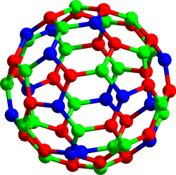
Figure 11: Division of the atoms of a C₆₀ molecule in groups (represented by different colors) whose pseudo-potential spheres do not overlap.

In Fig. 12, we plot the throughput obtained by the non-local potential implementation for a $\beta$-cyclodextrin molecule. The Nvidia card shows a good performance, 46 GFlops, only when large blocks of orbitals are used. The AMD card has a similar behavior, but the performance is much lower, with a maximum of 11 GFlops. This is a clear example of how our approach is an effective way of increasing the performance that can be obtained from the GPU. As this is a complex routine, and our current implementation is very basic, we suspect that a more sophisticated and optimized version could significantly increase the numerical performance of this part of the application of the KS Hamiltonian, in particular for the AMD GPU.

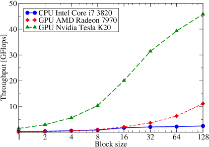
Figure 12: Numerical throughput of the application of the non-local potential as a function of the size of the block of orbitals (block-size). Calculation for $\beta$-cyclodextrin with 256 orbitals and 260k grid points.

VI Orthogonalization and subspace diagonalization

Given a set of orbitals, $\left\{\varphi_{k}\right\}$, the orthogonalization process generates a new set of orthogonal orbitals, $\left\{\bar{\varphi}_{k}\right\}$, as a linear combination of the original ones. Our implementation of the orthogonalization procedure is based on the Cholesky decomposition and other matrix linear algebra operations Kresse and Furthmüller (1996). For CPUs blas and lapack provide an efficient and portable set of routines to perform these operations. For GPUs, we use the OpenCL blas implementation provided by AMD as part of the Accelerated Parallel Processing Math Libraries (APPML).

The first step of the orthogonalization is to calculate the overlap between orbitals,

$$S_{jk}=\langle\varphi_{j}|\varphi_{k}\rangle\ .$$ (5)

Our first approximation to this problem was to use the orbitals-block approach to calculate the matrix $S$, by dividing it into sub-matrices, where each sub-matrix corresponds to the dot product between all the elements of two blocks of orbitals; however, this scheme is not efficient as it reduces the amount of data reuse in the matrix multiplication Wadleigh and Crawford (2000).

We have found that a much more efficient approach is to first copy the data to an array where all the coefficients corresponding to different orbitals are contiguous in memory, then we can use blas to calculate $S$ as a rank k operation. To avoid allocating a full copy of all the orbitals, we perform the operation for a set of points at a time. Effectively, we are switching from a block-of-orbitals representations to a block-of-points approach. Once $S$ is calculated, we need to factorize it into a $U^{\dagger}U$ form using a Cholesky decomposition Benoit (1924). In our implementation, this operation is done on the CPU using lapack. However, this is not an issue in our current implementation, since the cost of the decomposition is much smaller than other operations.

From the upper-triangular matrix $U$, given by the Cholesky decomposition, we can obtain the new set of orthogonal orbitals from the linear equation

$$\sum_{k}U_{jk}\bar{\varphi}_{k}({\bm{r}})={\varphi}_{j}({\bm{r}})\ .$$ (6)

Since $U$ is triangular, the solution of the linear problem is a simple operation that is done by blas. As this procedure mixes all states we cannot use the blocks-of-orbitals approach, instead we switch again to the blocks-of-points representation.

In Fig. 13 we show the performance obtained for our implementation of the orthogonalization procedure. The GPU speed-up is not very large with respect to the CPU. As this operation is based on linear algebra operations, we attribute the poor speed-up to difference in the linear algebra libraries. While for CPUs blas implementations are quite mature, the implementation of linear algebra operations on a GPU is still a field of active study, in particular for the solution of triangular systems Ries et al. (2012), like eq. (6).

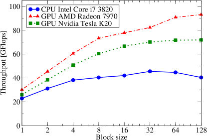
Figure 13: Numerical throughput of the orthogonalization procedure as a function of the size of the block of orbitals (block-size) for different processors. Calculation for $\beta$-cyclodextrin with 256 orbitals and 260k grid points.

The procedure for subspace diagonalization is very similar in form to the orthogonalization. It is used by diagonalization algorithms for sparse matrices to resolve between eigenvectors that have close eigenvalues. The first step in subspace diagonalization is to generate the representation of the Hamiltonian in the subspace of the approximated orbitals, $\left\{\varphi_{k}\right\}$,

$$h_{jk}=\langle\varphi_{j}|H|\varphi_{k}\rangle\ .$$ (7)

As in the case of the matrix $S$ for the orthogonalization, we perform this operation by blocks of points. This time we need to apply the Hamiltonian to the orbitals first, and then calculate the dot products as a matrix multiplication.

Once the subspace Hamiltonian is calculated, it is diagonalized to obtain the matrix of its eigenvectors, $\xi_{jk}$. As in the case of the Cholesky decomposition, this dense-matrix diagonalization is done by the CPU. This is not a performance issue for the systems studied in this article, but for larger systems, the dense eigensolver, that scales as $O(n^{3})$, could consume a considerable part of the computation time.

Once the subspace Hamiltonian is diagonalized, the new set of orbitals, $\left\{\bar{\varphi}_{k}\right\}$, is generated by rotating the old set by the eigenvector matrix,

$$\bar{\varphi}_{k}({\bm{r}})=\sum_{j}\xi_{jk}\,{\varphi}_{j}({\bm{r}})\ .$$ (8)

Since this rotation mixes all orbitals, we follow a similar procedure as we do in eq. (6) for the orthogonalization. The only difference is that in this case we directly multiply by the matrix instead of its inverse.

Fig. 14 shows the performance obtained for the subspace diagonalization. In this case the GPU speed-up is larger than for the orthogonalization case, probably because this routine is based on our implementation of the KS Hamiltonian, and on matrix-matrix multiplications, that in general are simpler to optimize and parallelize than other linear algebra operations.

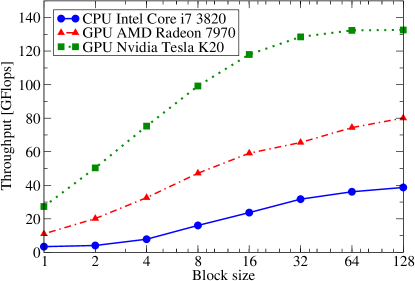
Figure 14: Numerical throughput of the subspace-diagonalization procedure as a function of the size of the block of orbitals (block-size) for different processors. Calculation for $\beta$-cyclodextrin with 256 orbitals and 260k grid points.

VII The Hartree potential

Other operation that we execute on the GPU is the calculation of the Hartree potential by solving the Poisson problem, eq. (3). This equation also appears in other contexts in electronic structure simulations, for example, in the calculation of approximations to the exchange term Perdew and Zunger (1981); *Umezawa2006; *Andrade2011, in the calculation of integrals that appear in Hartree–Fock or Casida theories Shang et al. (2010), or to impose electrostatic boundary conditions Tan et al. (1990); *Luscombe1992; Klamt and Schuurmann (1993); *Tomasi1994; Olivares-Amaya et al. (2011); *Watson2012.

The Poisson equation can be solved by different methods in linear or quasi-linear time Greengard and Rokhlin (1997); *Kutteh1995; Briggs (1987); *Beck1997; Cerioni et al. (2012); Garcia-Risueno et al. (2013). In our GPU implementation we use an approach based on fast Fourier transforms (FFTs), as it is quite efficient and simple to implement. By using FFTs, in principle we are imposing periodic boundary conditions to the electrostatic potential. We can, however, find the free-boundary solution by enlarging the FFT grid and using a modified interaction kernel Rozzi et al. (2006).

The solution process involves several steps. The first one is to copy the density from the arbitrarily-shaped grid to a cubic grid, where we perform the forward FFT. The result is the density in Fourier space, that is multiplied by the Coulomb-interaction kernel. After an inverse FFT, we obtain the Hartree potential, that is copied back to the arbitrarily-shaped grid. Since we only need to solve a single Poisson equation, independently of the size of the system, we cannot use the block approach in this case. The essential component of this solver is an FFT implementation, for GPUs, we use the clAMDFft library provided by AMD. For CPUs we use the multi-threaded FFTW library Frigo and Johnson (2005).

In Fig. 15, we show the performance of our GPU based Poisson solver for different system sizes. For the AMD card, the GPU version outperforms the CPU version, in some cases by a factor of 7. For the Nvidia GPU the speed-up is smaller, probably because the library has not been explicitly optimized for this GPU. The step structure seen on the plot is caused by the fact that FFTs cannot be performed efficiently over grids of any size: the grid dimension in each direction must be a product of certain values, or radices, that are determined by the implementation. If a grid dimension is not valid, the size of the grid is increased. Since the CPU implementation is more mature and supports more radices, the steps are smaller than the GPU implementation that only supports radices 2 and 3 . So, it is reasonable to expect that as the GPU-accelerated FFT implementations improve, the numerical performance of the calculation of the Hartree potential will increase.

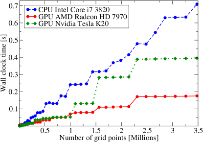
Figure 15: Comparison of the computational time required for solving the Poisson equation using FFTs as a function of the number of grid points. The data is originally on main memory, so the time required to copy the input data to the GPU and copy back the result is included. The number of points corresponds to the grid used by octopus, the FFT grid has a larger number of points.

VIII Other operations

In the previous sections we have described the main operations that we have implemented on the GPU. There are several simpler operations that also need to be performed on the GPU. These operations include basic operations between orbitals, like copies, linear combinations, and dot products. All of them are implemented on the GPU using the block-of-orbitals approach to improve performance. In fact, we have found that it is necessary to pay attention to the parallelization of most of the operations performed on the GPU, as a single routine that is not properly parallelized can spoil the numerical performance of the entire code.

In our current implementation, there are two procedures that are still done by the CPU, as they would require a considerable effort to implement on the GPU, but have a minor impact in numerical performance. The first one is the evaluation of the XC potential. This is a local operation that is straightforward to parallelize and should perform well on the GPU. The problem is that there is large number of XC approximations, each one involving complex formulas Marques et al. (2012) that would need to be implemented on the GPU. The second procedure that is executed on the CPU is the initialization of the molecular orbitals by a linear combination of the atomic orbitals obtained from the pseudo-potentials. The reason is that we use a spline interpolation to transfer the orbitals to the grid, which depends on the GSL library Galassi et al. (2003) that is not available on the GPU.

IX Accuracy

The strategy presented in this article does not imply a reduction in the precision of the calculations with respect to the original real-space DFT implementation. There are, however, some factors that could produce some numerical differences in the results.

In a sparse eigensolver, usually the eigenvectors are only converged until their error goes below a certain threshold, to avoid wasting computational time in over-converging some eigenvectors. In our implementation, iterations are only stopped when a whole block of eigenvectors is below the threshold. This makes the code simpler and avoids thread divergence, but introduces a dependency of the results on the block-size.

Another source of differences in the results is the calculation of the Hartree potential. Since the number of prime factors supported by the GPU FFT library is smaller than the CPU implementation, the size of the FFT grid can be larger for the GPU. However, as in both cases the grid is large enough to eliminate periodicity effects, the change in the results due to this difference is minimum.

Finally, there might be some differences in the numerical operations. While we use double precision for all operations and both GPUs used for the tests are IEEE-754 compliant, there might be differences in the finite precision arithmetic from fused multiply addition (FMA) operations, that are not available in the tested CPU, and due to different ordering of operations.

In our tests with different molecules we observe that the difference in the total energy between CPU and GPU calculations is on average 0.1 millihartree with a maximum of 0.5 millihartree. This is difference is caused mainly by the different size of FFT grids used by the CPU and GPU implementations of the Poisson solver. The difference between the energy computed with the Nvidia GPU with respect to the AMD GPU is on average 0.008 millihartree with a maximum of 0.08 millihartree. The variation of the total energy with the block-size is well below this values.

X Numerical performance

In this section we evaluate the numerical performance of our implementation and how it depends on the size of the blocks of orbitals or the size of the molecular systems. For this analysis we use several parameters: the throughput, the total calculation time for a single-point energy calculation, the speed-up with respect to the CPU implementation, and the comparison with a second GPU implementation.

X.1 Block-size

We start our performance analysis by studying how the block-size influences execution performance. In Fig. 16 we plot, for the $\beta$-cyclodextrin molecule, both the numerical throughput obtained for the SCF loop and the total execution time as a function of the size of the blocks of orbitals. For the CPU the optimal block-size is 16, with a second local optimum for block-size 256. For GPUs, increasing the block-size always improve performance up to size 128, that is the limit imposed by the GPU memory. This shows how the block approach produces a significant improvement with respect to working with a single orbital at a time (the block-size 1 case).

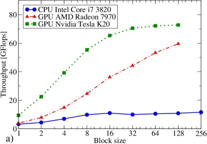
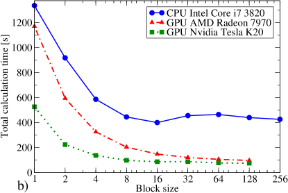
Figure 16: Performance of our CPU and GPU implementations as a function of the size of the block of orbitals (block-size). a) Numerical throughput of the self-consistency cycle. b) Total execution time for a single-point energy calculation. Simulation for $\beta$-cyclodextrin with 256 orbitals and 260k grid points.

X.2 Molecule size

We now focus our attention on how our GPU implementation performs for molecules of different sizes. For this test we have selected a set of 40 molecules, listed in table 1. In this respect, we would like to assert that we did not select the set of molecules based on any performance-related criterion, we just aimed to have a set of molecules composed mainly of first and second row elements with different numbers of valence electrons and that could fit in the memory of our GPUs.

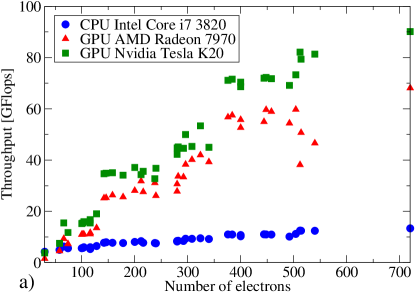
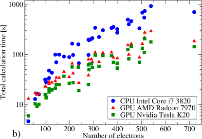
Figure 17: Performance of our CPU and GPU implementations for a set of 40 molecules of different sizes. a) Numerical throughput of the self-consistency cycle. b) Total execution time for a single-point energy calculation. The list of molecules and the calculation times are given in table 1.

Table 1: List of systems used for the performance studies done in this article. For each molecule we include the number of valence electrons, the number of grid points used in the simulation, the computational times for octopus with three different processors: CPU Intel Core i7 3820 (CPU), GPU AMD Radeon HD 7970 (AMD) and GPU Nvidia Tesla K20 (Nvidia), and calculation time for terachem with the Nvidia Tesla K20 GPU (Terachem). The geometry for each molecule can be found as supplementary information. ^aThese molecules were obtained from the Harvard Clean Energy Project (CEP) Hachmann et al. (2011).

System		Calculation size		Single-point calculation time [s]
Stoichiometry	Description	Electrons	Points [1/1000]	CPU	AMD	Nvidia	Terachem
C6H6	benzene	30	37.3	4.6	13.0	5.9	2.0
C10H18	cis-decalin	58	62.5	12.8	16.9	10.3	6.8
C14H10	anthracene	66	63.0	16.3	15.7	9.2	7.6
C8H10N4O2	caffeine	74	63.1	15.9	16.1	10.0	8.7
C16H24O2	palmitoyl	100	93.2	31.3	22.8	15.7	15.1
C18H24	cis-retinal	102	96.5	31.0	22.7	15.6	17.4
(H2O)13	water cluster	104	83.7	27.7	20.9	13.5	8.2
C20H24O2	ethinyl estradiol	116	99.1	33.6	25.6	17.8	24.1
C18H32O2	linoleic acid	116	122.7	47.5	28.5	20.5	14.4
C22H28O2	etonogestrel	128	107.3	43.1	27.3	19.5	30.0
C26H16O3S	molecule from CEPa	142	110.0	62.7	29.3	21.1	24.6
C29H20N2	molecule from CEPa	146	119.9	69.5	34.5	25.0	30.4
C34H22	diphenylpentacene	158	131.2	99.0	34.1	24.8	33.8
C22H30N6O4S	sildenafil citrate	178	137.8	90.6	45.3	36.6	41.3
CH4(H2O)24	methane + water	200	132.6	88.2	35.5	26.4	27.8
C40H52	carotene	212	206.0	163.9	65.8	56.2	42.1
C48H24	kekulene	216	147.6	97.0	41.9	27.2	49.2
C44H54Si2	TIPS-pentacene	238	182.8	158.6	59.6	55.5	68.6
C60	fullerene	240	102.4	66.6	27.0	18.9	76.6
C70	fullerene	280	113.1	97.2	38.2	24.9	128.3
C51H33N5O3	porphyrin	280	209.8	196.7	79.5	61.8	105.4
C58H32S3	molecule from CEPa	282	214.9	192.0	64.8	49.5	82.0
C41H40N8O8	carbazole complex	292	192.3	203.5	80.4	64.7	126.2
C60H32S4	DAT-thiophane dimer	296	213.7	211.6	70.4	54.5	78.9
C42H83NO8P	phosphatidylcholine	308	283.9	340.8	109.7	96.4	95.7
C45H51NO15	taxol	324	219.0	222.6	71.2	57.6	141.1
C50H238MgN4O5	chlorophyll	340	269.8	303.9	107.8	94.9	174.5
C58H48N8O12	methotrexate complex	376	238.1	337.4	110.1	94.3	135.4
C36H60O30	$\alpha$-cyclodextrin	384	222.9	354.9	86.6	69.2	89.6
C100	fullerene	400	160.8	272.2	64.9	53.1	194.2
C60(H2O)20	fullerene + water	400	200.5	319.2	83.7	66.3	225.2
C54H90N6O18	valinomycin	444	293.6	494.3	152.5	124.5	185.6
C42H70O35	$\beta$-cyclodextrin	448	259.5	401.0	99.5	81.6	100.6
C62H63N15O12	methotrexate complex	458	265.4	461.6	163.1	145.0	331.1
C122H4	fullerene dimer	492	198.3	331.4	87.2	69.6	344.0
C114H48	graphite cluster	504	277.8	684.1	162.6	132.5	672.4
C48H80O40	$\gamma$-cyclodextrin	512	290.9	543.3	216.8	109.5	131.0
C68H76N13O16P	cAMP complex	514	327.4	734.6	273.0	206.7	334.1
C68H318Na2O20P2	phospholipid	540	404.7	925.8	291.3	177.8	808.8
C180	fullerene	720	267.8	699.2	188.9	141.8	461.1

In Fig. 17, we show, for the molecules in our set, the performance measured as throughput of the SCF cycle and total computational time as a function of the number of electrons. As expected, the computational time tends to increase with the number of electrons, but there is a strong variation from system to system. This variation is mainly explained by the physical size of each molecule, that determines the size of the grid that is used in the simulation. The number of iterations required for eigensolver and self-consistency convergence can also change from one system to the other, affecting the total calculation time. From Fig. 17a is clear that as the size of the system increases, the GPU becomes more efficient, with a maximum throughput of 90 GFlops for the largest molecule tested, C₁₈₀.

We now measure the speed-up of the GPUs with respect to the CPU version. In Fig. 18a we plot the speed-up measured using the total computational time. The maximum value we get is 5.2x for the Nvidia GPU and 4.2x for the AMD GPU. If we only consider the time spent in the SCF cycle and ignore the initialization time, the speed-up is 8.0x for the Nvidia GPU and 5.2x for the AMD GPU, the curve also becomes more regular, hinting that much of the variation in the computational time for systems with similar number of electrons comes from initialization routines.

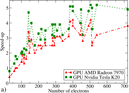
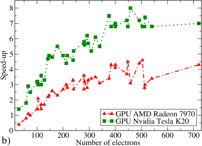
Figure 18: Speed-up of the GPU calculation with the respect to the CPU for different molecules as a function of the number of valence electrons. a) Speed-up calculated from the total calculation time. b) Speed-up computed from the time spent in the SCF-cycle (without considering initializations). The reference CPU is an Intel Core i7 3820 using 8 threads.

While the speed-ups are not as large as some that have been reported in the literature, there are several factors to consider when analyzing GPU speed-ups. First of all, the maximum speed-up we could obtain is given by the peak-performance ratio between the GPU and the CPU, which is approximately 8x for and the AMD GPU and 10x for the Nvidia card. If performance is limited by the memory bandwidth, then the maximum speed-up is reduced to 5x (AMD) or 6x (Nvidia). The CPU code taken as reference is also important. In this case we are comparing code that uses the similar optimization strategies on the CPU and the GPU, and in both the cases it has been parallelized to use all the execution units available on each processor. This is not the case, for example, when a full GPU is compared against a single core of a CPU.

X.3 Comparison with Terachem

In order to make an exhaustive evaluation of the performance of our approach, we compare it with another GPU-accelerated DFT implementation, the terachem code Ufimtsev and Martínez (2008a, b); *Ufimtsev2009a; *Ufimtsev2009b; *Luehr2011. Terachem uses Gaussian type orbitals (GTOs) as a basis for the expansion of the molecular orbitals: the traditional approach used in quantum chemistry. Terachem has been extended to perform different types of simulations like excited states Isborn et al. (2011) or ab-initio molecular dynamics Ufimtsev et al. (2011), and thanks to the computational power offered by GPUs, it has been used to study challenging systems like large proteins Kulik et al. (2012); *Isborn2012.

Since octopus and terachem use very different simulation techniques, we take great care in making a significant comparison. The main issue is to select discretization parameters that produce a similar level of approximation. We take as reference the caffeine molecule, C₈H₁₀N₄O₂ in the Becke-Lee-Yang-Parr (BLYP) XC approximation Becke (1988); *Lee1988; *Miehlich1989. In terachem we select the 6-311g* basis that has an error in the total energy of 5 millihartree per atom, with respect to a calculation with the aug-cc-pvqz basis. We then look for grid parameters that give a similar error, this time taking as reference the converged real-space result. The selected grid is a union of spheres of radius 5.5 Bohr around each atom and a spacing of 0.41 Bohr. However, the real-space approach has an additional approximation, as it requires pseudo-potentials so that the ionic potential is smooth enough to be represented in a uniform grid. To minimize the effect of this difference in computation time and to compare the actual implementation, we test molecules composed mainly of first and second-row elements.

In Fig. 19, we compare the timings for both codes for the same set of systems used in section X.2 (table 1). We show the comparison between absolute times and also the relative performance between the two DFT implementations. We can see that terachem tends to be faster for smaller systems, while octopus has an advantage for systems with more than 100 electrons. It is difficult to generalize these results due to the different simulation approaches and their different strengths and weaknesses. For example, our current implementation will certainly be much slower than terachem for hybrid HF-DFT XC approximations Becke (1993) due to the cost of applying exact-exchange operator in real-space. However, we can conclude that for pure DFT calculations the real-space method can compete with the Gaussian approach, and can outperform it for some systems.

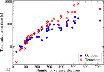
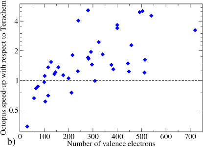
Figure 19: Numerical performance comparison between our GPU implementation (octopus) and the terachem code. a) Comparison of the total calculation time as a function of the number of valence electrons. b) Speed-up of our implementation with respect to terachem (run time of terachem divided by the run time of octopus). The calculations are single-point energy evaluations performed on a set of 40 molecules, running on a Nvidia Tesla K20 GPU. The list of molecules and the calculation times are given in table 1.

XI Conclusions

We have presented an approach for the implementation of real-space density functional theory on GPUs. What we have shown is much more than a re-implementation of the code in GPU language, but a scheme designed to perform DFT calculations efficiently on massively parallel processors.

Our approach is based on using blocks of KS orbitals as the basic data object. This provides the GPU with enough data to perform efficiently, something that would be harder to achieve by working on single orbitals at a time. However, this approach is not applicable or does not work efficiently for all operations, so in other cases a block-of-points strategy is used. Many of these techniques are applicable to other DFT discretization approaches, especially those based on sparse representations like plane-waves or wavelets.

The efficiency of our approach is analyzed by examining several parameters. We achieve a considerable throughput and speed-up with respect to the CPU version of octopus. More importantly, in comparison to a GPU-accelerated implementation of DFT based on Gaussian basis sets, we find that calculation times are similar, with our code being faster for several of the systems that were tested. This is not to be taken lightly, as the GTO approach has been designed and constantly improved with the specific purpose of efficiently modeling molecular systems. The real-space method, on the other hand, is a more general approach used to study different types of partial differential equations.

We can conclude that the real-space formulation provides a good framework for the implementation of DFT on GPUs, making real-space DFT an interesting alternative for electronic structure calculations, as it offers good performance, systematic control of the discretization and the flexibility to study many classes of systems, including both periodic and finite systems.

A particular advantage of real-space DFT is its potential for large scale parallelization in distributed memory systems with tens of thousands of processors Andrade et al. (2012a); Enkovaara et al. (2010); Hasegawa et al. (2011). This is something we want to apply in future work, by exploring the combination of in-processor (OpenCL) and distributed memory (MPI) parallelization for DFT calculations on GPU-based supercomputers.

XII Computational methods

Our numerical implementation is included in the Octopus code Marques et al. (2003); Castro et al. (2006); Andrade et al. (2012a) and it is publicly available under the GPL free-software license oct . The calculations were performed with the development version (octopus superciliosus, svn revision 10562). GPU support is also available in the 4.1 release of Octopus.

Since octopus is written in Fortran 95, we wrote a wrapper library to call OpenCL from that language. This library is called FortranCL and it is available as a standalone package under a free-software license Andrade (2011).

All calculations were performed using the default pseudo-potentials of octopus, filtered to remove high-frequency components Tafipolsky and Schmid (2006). The grid for all simulation is a union of spheres of radius 5.5 Bohr around each atom with a uniform spacing of 0.41 Bohr.

The GTO calculations were done with terachem (version v1.5K) with the 6-311g* basis and dftgrid = 1. All other simulation parameters were kept in its default values. For all calculations we used the BLYP XC functional Becke (1988); *Lee1988; *Miehlich1989.

The system used for the tests has an Intel Core i7 3820 CPU, which has 4 cores running at 3.6 GHz that can execute 2 threads each. The CPU has a quad-channel memory subsystem with 16 GiB of RAM running at 1600 MHz. The GPUs are a AMD Radeon HD 7970 with 3 GiB of RAM and Nvidia Tesla K20c with 5 GiB (ECC is disabled, as the other processors do not support ECC). Both GPUs are connected to a PCIe 16x slot, the AMD card supports the PCIe 3 protocol while the Nvidia card is limited to PCIe 2. Octopus was compiled with the GNU compiler (gcc and gfortran, version 4.7.2) with AVX vectorization enabled. For finite-difference operations, CPU vectorization is implemented explicitly using compiler directives. We use the Intel MKL (version 10.3.6) implementation of blas and lapack that is optimized for AVX. We use the OpenCL implementation from the respective GPU vendor: the AMD OpenCL version is 1084.4 (VM) and the Nvidia one is 310.32 (OpenCL is not used for the CPU calculations). All tests are executed with 8 OpenMP threads.

Total and partial execution times were measured using the gettimeofday call. The throughput is defined as the number of floating point additions and multiplications per unit of time. The number of operations for each procedure is counted by inspection of the code. For terachem the total execution time is obtained from the program output.