A linear distribution of orbits in compact planetary systems?

Abstract

We report a linear ordering of orbits in a sample of multiple extrasolar planetary systems with super-Earth planets. We selected $20$ cases, mostly discovered by the Kepler mission, hosting at least four planets within $\sim 0.5\,\mbox{au}$. The semi-major axis $a_{n}$ of an $n$-th planet in each system of this sample obeys $a(n)=a_{1}+(n-1)\,\Delta\,a$, where $a_{1}$ is the semi-major axis of the innermost orbit and $\Delta\,a$ is a spacing between subsequent planets, which are specific for a particular system. For instance, the Kepler-33 system hosting five super-Earth planets exhibits the relative deviations between the observed and linearly predicted semi-major axes of only a few percent. At least half of systems in the sample fulfill the linear law with a similar accuracy. We explain the linear distribution of semi-major axes as a natural implication of multiple chains of mean motion resonances between subsequent planets, which emerge due to planet–disk interactions and convergent migration at early stages of their evolution.

1 Introduction

The Kepler photometric mission (Borucki et al., 2010) brought many discoveries of multiple low-mass planetary systems. There are several known systems with four or more super-Earths and/or Neptune/Uranus mass planets. In particular there are the Kepler-11 system with six planets (Lissauer et al., 2011), five-planet systems Kepler-33 (Lissauer et al., 2012), Kepler-20 (Gautier et al., 2012) and Kepler-32 (Fabrycky et al., 2012). There are also a few systems with five candidate planets: KOI-435 (Ofir & Dreizler, 2012), KOI-500, KOI-505 (Borucki et al., 2011) and several more four-planet systems. Configurations of this type were first discovered with Doppler spectroscopy, e.g., Gliese 876 (Rivera et al., 2010), Gliese 581 (Forveille et al., 2011), HD 10180 (Lovis et al., 2011) and HD 40307 (Tuomi et al., 2013). In the Gliese 876 system, however, two of the companions are jovian planets, similarly to the Kepler-94 system. All studied systems, with a few discussed furthermore, host at least four planets with orbital semi-major axes $\lesssim 0.5\,\mbox{au}$.

These discoveries raise a question on mechanisms leading to such compact ordering of the planetary systems, and simultaneously providing their long-term stability. Our recent study of the Kepler-11 system (Migaszewski et al., 2012) revealed that this configuration of six super-Earths is chaotic, and its marginal, long-term dynamical (Lagrangian) stability is most likely possible due to particular multiple mean-motion resonances between the planets. In the sample quoted above, we may pick up multiple configurations even more compact, and bounded to the distance as small as $0.08\,\mbox{au}$, e.g., Kepler’s KOI-500 with five planets. The orbital architecture of planetary systems of this class recalls the hypothesis of the Packed Planetary Systems (PPS, Barnes & Raymond, 2004), though originally formulated for configurations with jovian companions. In the jovian mass range, the orbital stability of multiple systems is statistically preserved, if planets in subsequent pairs with semi-major axes $a_{1},a_{2}$ and masses $m_{1},m_{2}$ are separated by more than $K\sim 4,5$ mutual Hill radii $R_{H,M}$, where $R_{H,M}=(1/2)(a_{1}+a_{2})[(m_{1}+m_{2})/(3m_{*})]^{(1/3)}$ and $m_{*}$ is the mass of the parent star (Chatterjee et al., 2008). However, $R_{H,M}$ in the above systems is of the order of $10^{-3}$ au, hence their typical separation is at least one order of magnitude larger, $K\sim 10$, for the outermost pairs of planets, while for the innermost planets $K\sim 30$–$50$. A study of systems with 1 Earth-mass planets orbiting a Sun-like star conclude that the stability is maintained for $K$ roughly larger than 10-13 (Smith & Lissauer, 2009). This seems in accord with the analysis of the Kepler-11 (Migaszewski et al., 2012) and similar systems which reveals, that likely they evolved into a particular architectures helping to maintain the stability. Indeed, due to small eccentricities, these systems unlikely suffered planet-planet scattering, often quoted in the literature to explain the observed eccentricity distribution in the sample of multiple extrasolar systems (e.g. Raymond et al., 2009). In the light of the PPS hypothesis, the multiple, compact systems with super-Earths will be classified as packed multiple-planet systems, from hereafter. In this Letter, we report a detection of a linear ordering of the planets with their number (index) and argue that such particular architecture might stem from the planetary migration.

2 A prototype case: the Kepler-33 system

The Kepler-33 system hosts five planets. For the parent star mass $m_{0}=(1.29\pm 0.12)\,\mbox{M}_{\sun}$ (see caption to Table 1 for references to all discussed systems) and the reported orbital periods, we computed the semi-major axes of the planets, $a_{n}$, where $n=2,3,4,5,6$. The plot of $a_{n}$ against $n$ (the top left-hand panel of Fig. 1) reveals a clear linear correlation $a(n)=0.024+0.047\,(n-1)$ (shown as a green line). We start the sequence of indexes from $2$ rather than from $1$ to have $a_{1}\in[0,\Delta\,a)$. We want this condition to be fulfilled in all studied examples. The uncertainties of the best-fit parameters $a_{1},\Delta\,a$ (accompanied by other quantities introduced below) are given in the first row of Table 1. All of $a_{n}$ are very close to the line on the $(n,a_{n})$-graph. In the sample of multiple Kepler systems, we found a few other systems exhibiting a similar dependence of the semi-major axes on the planet index. To express deviations between observed and predicted semi-major axis (O-C) of a planet in a given system, we introduce $\Delta_{n}\equiv[a_{n}-a(n)]/a_{n}$ and $\bar{\Delta}_{n}\equiv[a_{n}-a(n)]/\Delta\,a,$ which are the (O-C) scaled by $a_{n}$ and $\Delta\,a$, respectively. The top-left panel of Fig. 1 is labeled by $\Delta_{n}$ and $\bar{\Delta}_{n}$ expressed in percents, close to each red filled-circle marking a particular $a_{n}$. Values of $\Delta_{n}$ are given above the linear graph, and $\bar{\Delta}_{n}$ below the graph. To measure the ”goodness of fit” of the linear model for a whole $N$-planet system, we define $\delta\equiv\big{[}\frac{1}{N}\sum_{i=1}^{N}\bar{\Delta}_{n(i)}^{2}\big{]}^{1/2}\times 100\,\%,$ where $n(i)$ is an index given to $i$-th planet. Therefore, $\delta$ is equivalent to the common rms scaled by the spacing parameter $\Delta a$. When the indexes $n(i)$ for subsequent planets of the Kepler-33 are $2,3,4,5,6$, the resulting $\delta\approx 6.1\,\%$. We did not find any better linear fit parameters and planets numbering. However, in other cases, as shown below, non-unique solutions may appear for different $\Delta\,a$.

To find the best-fit combination of the $a_{1},\Delta a$ and a sequence of indexes $\left\{n(i)\right\}_{i=1}^{i=N}$, for each studied system, we perform a simple optimization. We fix a point in the $(a_{1},\Delta\,a)$–plane, where $a_{1}\in[0,\Delta\,a)$ and look for a set of indexes $n(i)$ providing $\min\bar{\Delta}_{n(i)}$. The results for the Kepler-33 system are illustrated in the top left-hand panel of Fig. 2 in the form of one-dimensional scan over $\Delta a$.

Table 1: The results of analysis of a sample of $21$ systems. References: $1$: Lissauer et al. (2012), $2$: Ofir & Dreizler (2012), $3$: Borucki et al. (2011), $4$: Fabrycky et al. (2012), $5$: Tuomi et al. (2013), $6$: Hirano et al. (2012), $7$: Weiss et al. (2013), $8$: Lissauer et al. (2011), $9$: Forveille et al. (2011), $10$: Gautier et al. (2012), $11$: Rivera et al. (2010), $12$: Lovis et al. (2011).

star	$m_{0}[\mbox{M}_{\sun}]$	$N$	ref.	$\Delta\,a\,[\mbox{au}]$	$a_{1}\,[\mbox{au}]$	$\delta[\%]$	$f_{2/3}[\%]$	$f_{1}[\%]$	sequence
Kepler-33	$1.29\pm 0.12$	$5$	$1$	$0.0466\pm 0.0012$	$0.024\pm 0.004$	$6.1$	$5.8$	$1.8$	$2-3-4-5-6$
KOI-435	$0.9$	$5$	$2$	$0.0507\pm 0.0012$	$0.0419\pm 0.0033$	$6.9$	$8.0$	$2.5$	$1-2-3-4-6$
KOI-1955	$1.0^{*}$	$4$	$2$	$0.0497\pm 0.0015$	$0.025\pm 0.004$	$6.0$	$14.4$	$6.6$	$1-3-4-5$
KOI-719	$0.68$	$4$	$3$	$0.0291\pm 0.0004$	$0.0155\pm 0.0017$	$4.3$	$8.0$	$3.6$	$2-3-6-8$
KOI-408	$1.05$	$4$	$3$	$0.03006\pm 0.00035$	$0.0157\pm 0.0013$	$3.0$	$3.8$	$1.7$	$2-3-4-7$
KOI-671	$0.96$	$4$	$3$	$0.02428\pm 0.00082$	$0.001\pm 0.003$	$5.7$	$11.3$	$5.2$	$3-4-5-6$
Kepler-32	$0.58\pm 0.05$	$5$	$4$	$0.01952\pm 0.00036$	$0.0132\pm 0.0012$	$6.5$	$6.7$	$2.1$	$1-2-3-4-7$
KOI-500	$0.66$	$5$	$3$	$0.0146\pm 0.0006$	$0.004\pm 0.002$	$10.2$	$23.2$	$7.9$	$2-3-4-5-6$
HD 40307	$0.77\pm 0.05$	$6$	$5$	$0.02795\pm 0.00016$	$0.0229\pm 0.0015$	$7.2$	$4.1$	$0.9$	$2-3-5-7-9-22$
KOI-730	$1.07$	$4$	$3$	$0.01400\pm 0.00044$	$0.0071\pm 0.0033$	$8.3$	$26.8$	$12.8$	$6-7-9-11$
KOI-94	$1.25\pm 0.40$	$4$	$6,7$	$0.0637\pm 0.0027$	$0.0437\pm 0.0062$	$8.8$	$29.0$	$13.8$	$1-2-3-5$
Gliese 581	$0.31\pm 0.02$	$5$	$9$	$0.01469\pm 0.00013$	$0.013\pm 0.001$	$7.3$	$9.7$	$3.1$	$2-3-5-10-15$
KOI-510	$1.03$	$4$	$3$	$0.0243\pm 0.0005$	$0.0184\pm 0.0022$	$7.4$	$21.4$	$10.1$	$2-3-5-9$
KOI-505	$1.01$	$5$	$3$	$0.01181\pm 0.00006$	$0.008\pm 0.001$	$9.8$	$20.3$	$6.9$	$4-6-7-10-33$
Kepler-31	$1.21\pm 0.17$	$4$	$4$	$0.0521\pm 0.0013$	$0.047\pm 0.006$	$8.0$	$24.8$	$11.8$	$2-3-5-8$
				$0.0807\pm 0.0033$	$0.008\pm 0.010$	$8.3$	$26.0$	$12.3$	$2-3-4-6$
Kepler-11	$0.95\pm 0.10$	$6$	$8$	$0.01427\pm 0.00011$	$0.0077\pm 0.0019$	$13.4$	$33.9$	$8.8$	$7-8-11-14-18-33$
				$0.0519\pm 0.0013$	$0.0453\pm 0.0051$	$11.7$	$22.5$	$5.5$	$2-2-3-4-5-9$
Kepler-20	$0.912\pm 0.035$	$5$	$10$	$0.0149\pm 0.0001$	$0.0027\pm 0.0011$	$7.9$	$11.8$	$3.8$	$4-5-7-10-24$
				$0.0232\pm 0.0003$	$0.0211\pm 0.0019$	$9.6$	$19.3$	$6.5$	$2-3-4-6-15$
KOI-623	$1.21$	$4$	$3$	$0.0353\pm 0.0027$	$0.024\pm 0.008$	$11.8$	$47.3$	$23.8$	$2-3-4-5$
				$0.0282\pm 0.0017$	$0.013\pm 0.007$	$12.2$	$49.4$	$24.9$	$3-4-5-7$
Gliese 876	$0.33\pm 0.03$	$4$	$11$	$0.1030\pm 0.0063$	$0.021\pm 0.012$	$9.5$	$33.5$	$16.1$	$1-2-3-4$
				$0.064\pm 0.003$	$0.015\pm 0.009$	$10.9$	$41.6$	$20.3$	$1-3-4-6$
HD 10180	$1.06\pm 0.05$	$5$	$12$	$0.0717\pm 0.0003$	$0.0597\pm 0.0027$	$4.8$	$3.0$	$1.0$	$1-2-4-7-20$
		$8$		$0.02246\pm 0.00006$	$0.0202\pm 0.0014$	$11.3$	$9.0$	$1.0$	$1-3-4-6-12-15-22-63$

Red color is for solutions for which minimal difference between subsequent indexes equal to $1$. For instance, a solution of a given $\Delta\,a$ corresponding to a sequence $1-2-4-6-7$ would be plotted in red, because differences between indexes $n(2)=2$ and $n(1)=1$ as well as $n(5)=7$ and $n(4)=6$ equals $1$. On the other hand, $\Delta\,a$ corresponding to a sequence $1-3-5-8-11$ would be plotted in black (minimal difference between indexes equals $2$ in this case). It is obvious that when $\Delta\,a$ is much smaller than the distance between planets forming the closest pair in a system, one can obtain apparently very low values of $\delta$. To avoid such artificial solutions, we limit our analysis to solutions from the red part of scans presented on Fig. 2.

2.1 Testing the linear ordering for known packed systems

The sample consists of $20$ systems (including Kepler 33). The results are gathered in Table 1. Its columns display the name of the star, its mass, the number of planets, the reference, $\Delta\,a$, $a_{1}$, $\delta$, $f_{2/3}$, $f_{1}$ (False Alarm Probabilities, FAPs, defined below) and a sequence of $n(i)$. A few planetary systems have more than one record. Figure 1 shows the $(n,a_{n})$-diagrams for $9$ chosen systems. For a reference, 1-dim scans of $\delta(\Delta\,a)$ are presented in Fig. 2. The choice of systems to be shown in Figs. 1 and 2 was made on basis of a few criteria, which are: as low $\delta$ and FAP as possible, and as few gaps as possible. Because this is a multiple-criteria choice it has to be, to some degree, arbitrary.

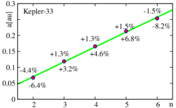
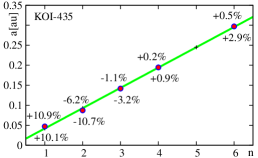
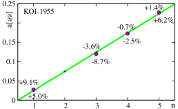
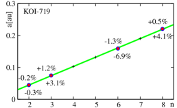
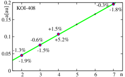
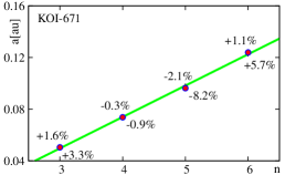
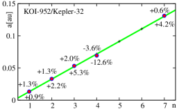
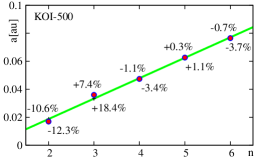
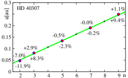
Figure 1: The $(n,a_{n})$-diagrams of the best-fit linear solutions computed for chosen planetary systems. See the text for details.

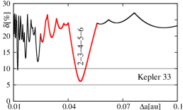
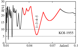
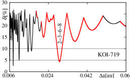
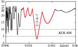
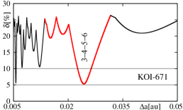
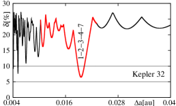
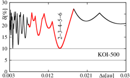
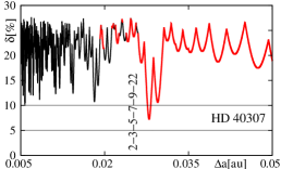
Figure 2: Goodness of the linear fit $\delta$ as a function of $\Delta\,a$. Each panel is for one system.

KOI-435 is a system with five planetary candidates in orbits of $a\lesssim 0.4\,\mbox{au}$ and the sixth object, for which only one transit was observed, is much more distant from the star. Here, we take into account only five inner candidates. Fig. 2 reveals that the linear model corresponds to the minimum of $\delta$ around $\Delta\,a\approx 0.05$ au, which is close to the value for the Kepler-33 system. The quality of this model is very good, $\delta\approx 7\,\%$. Indexes of the planets are $1-2-3-4-6$, hence there is a gap between planet 4 and planet 6. We did not find any better nor alternative solution. It is not yet possible to say if such a gap should be filled by yet undetected planet. The question is if such gaps are frequent outcomes of physical processes leading to discussed architecture. If they are rare one might expect a planet with $n=5$ in the KOI-435, otherwise we cannot make any predictions. Figure 1 shows $(n,a_{n})$-diagram for this sequence. This system seems very similar to the Kepler-33 system. A difference of $a_{1}$ means that the orbits of planets in KOI-435 are slightly shifted, when compared to the Kepler-33 orbits. In both cases, stellar masses are known with $\sim 10\,\%$ uncertainty, which propagates into $\sim 3\,\%$ uncertainty of $a_{n}$, as well as of $\Delta\,a$ and $a_{1}$.

We estimate, that the remaining $7$ systems shown in Fig. 2 obey the linear law similarly well. The most interesting example here is KOI-500 with five planets, which form a sequence $2-3-4-5-6$ (the same as Kepler 33). All planets reside within the distance of $0.08\,\mbox{au}$ from the parent star.

The Kepler-31 system (not shown in Fig. 2) of four candidate planets, exhibits non-unique solutions ($\Delta\,a\approx 0.052\,\mbox{au}$ and $\Delta\,a\approx 0.081\,\mbox{au}$). For both of them $\delta\approx 8\,\%$. Indexes of these models are $2-3-5-8$ and $2-3-4-6$, respectively. The next system, Kepler-11 has six planets. Two of its inner orbits are separated by only $\sim 0.015\,\mbox{au}$. Other orbits are separated by $\sim 0.05\,\mbox{au}$ except of the last one, which is relatively distant (separated by $\sim 0.2\,\mbox{au}$ from the preceding planet). There are two possible solutions: $\Delta\,a\approx 0.0154\,\mbox{au}$ ($\delta\gtrsim 13\,\%$) and $\Delta\,a\approx 0.052\,\mbox{au}$ ($\delta\approx 12\,\%$). For the second case the indexes are $2-2-3-4-5-9$, i.e., two innermost planets have the same number $2$. The parameters are almost the same as for KOI-435 and Kepler-31 (the first solution). The remaining members of the group of systems not shown in Fig. 2 exhibit relatively large $\delta$ or the best-fit models have usually many ”gaps”. Moreover, in some cases, more than one model is possible (see Tab. 1).

Having in mind systems with many gaps and/or large values of $\delta$, one might ask whether the linear ordering might be just a matter of blind coincidence, like the widely criticised Titius-Bode (TB) rule. To check the linear rule on statistical grounds, we applied the Monte-Carlo approach of Lynch (2003). He expressed the TB model in the logarithmic scale, which can be directly used in our case. We then analyse a random sample of $10^{7}$ synthetic orbits of $a_{n}=a_{1}+[(n-1)+k\,y_{n}]\Delta a,$ where $y_{n}\in[-0.5,+0.5]$ is chosen randomly, while $k>0$ is a scaling parameter. We optimize each synthetic system and compute the percentage of systems for which $\delta<\delta_{0}$, where $\delta_{0}$ is for the observed system. The resulting FAPs for $k=2/3$ and $k=1$ are displayed as $f_{2/3}$, and $f_{1}$ in Table 1, respectively. We conclude that the random occurrence of the linear ordering in unlikely ($f_{2/3}\lesssim 10\,\%$, $f_{1}\lesssim 5\,\%$) for approximately half of the sample. Nevertheless, these results are not definite, as the FAPs might depend on the sampling strategy (Lynch, 2003).

We would like to stress here that the linear ordering of orbits is not expected to be a universal rule which all systems would obey. We found that some of them are ordered according to this rule while some other systems from the sample are built differently. Our next step is to explain this.

3 Is the linear rule reflecting MMRs?

Since the linear spacing of orbits cannot be pure coincidence for all systems, there should be a physical mechanism leading to this particular ordering of them. Searching for possible explanations of this phenomenon, we found that it may appear naturally due to the inward, convergent migration of the planets interacting with the remnant protoplanetary disk. The migration of two planets in a gaseous disk has been studied in many papers (e.g., Papaloizou & Terquem, 2006; Szuszkiewicz & Podlewska-Gaca, 2012). It is known that the migration usually leads to trapping orbits into the mean motion resonances (MMRs). It is reasonable to foresee that systems with more planets might be trapped into chains of MMRs, see Conclusions. We ask now if there is any combination of MMRs between subsequent pairs of planets resulting in the linear spacing of the orbits.

There are no MMRs leading to the exact linear spacing of the orbits ($\delta=0$). However, we can pick up easily many different linear model possessing $\delta\sim 1\,\%$. We examined synthetic planetary systems of $5$ and $6$ planets involved in multiple MMRs. We searched for such combinations of MMRs which lead to the linear distribution of semi-major axes with no ”gaps”, like in the Kepler 33 case. We found many models with $\delta<4\,\%$. Let us quote some interesting examples. For a five-planet system, subsequent MMRs $7:3$, $5:3$, $3:2$ and $4:3$ corresponds to a sequence of indexes $2-3-4-5-6$ and $\delta\approx 2.4\,\%$. Actually, this is very similar to the Kepler 33 system. Its planets are close to the same resonances.

A proximity of a particular pair of planets $i$ and $i+1$ to a given MMR $q:p$, i.e., $P_{i+1}/P_{i}\approx q/p$ (where $q,p$ are relatively prime natural numbers), can be expressed through $\epsilon_{i,i+1}(q,p)\equiv\left({q\,P_{i}}/{p\,P_{i+1}}-1\right)\times 100\,\%.$ For Kepler 33 one finds $\epsilon_{{\mbox{\scriptsize b}},{\mbox{\scriptsize c}}}(7,3)\approx 0.4\,\%,\epsilon_{{\mbox{\scriptsize c}},{\mbox{\scriptsize d}}}(5,3)\approx 0.8\,\%,\epsilon_{{\mbox{\scriptsize d}},{\mbox{\scriptsize e}}}(3,2)\approx 2.7\,\%,\epsilon_{{\mbox{\scriptsize e}},{\mbox{\scriptsize f}}}(4,3)\approx 3.2\,\%,$ where the subsequent planets are called as b, c, d, e and f, respectively. Periods ratios of the first two pairs of planets are almost exactly equal to rational numbers $7/3$ and $5/3$. For two more distant pairs, deviations from $3/2$ and $4/3$ are slightly larger, still as small as $\sim 3\,\%$.

If, in accord with the linear law, there existed one more innermost planet, it would be involved in $7:1$ MMR with planet b. In such a case, the six-planet sequence would correspond to the MMRs chain of $7:1$, $7:3$, $5:3$, $3:2$, $4:3$ and $\delta\approx 2.2\%$. Yet other MMRs between planets $1$ and $b$ are possible ($6:1$, $8:1$, $9:1$, $11:2$), leading to $\delta<3\,\%$. One more example of six planets involved in low order MMRs are: $5:1$, $2:1$, $5:3$, $3:2$, $4:3$ with $\delta\approx 3.4\,\%$ (the first MMR could be also $6:1$, $9:2$); $7:1$, $5:2$, $5:3$, $3:2$, $4:3$ ($\delta\approx 3.4\,\%$); $9:2$, $9:4$, $5:3$, $3:2$, $4:3$ ($\delta\approx 3.6\,\%$); $6:1$, $7:3$, $7:4$, $3:2$, $4:3$ ($\delta\approx 3.6\,\%$). There are many other solutions with higher order resonances and/or larger $\delta$. The most frequent MMRs in such sequences are $3:2$, $4:3$, $5:2$, $5:3$, $2:1$ and $7:3$. Considering the 4:3 MMR, Rein et al. (2012) argue that it is difficult to construct this resonance on the grounds of the common planet formation scenario. However, Rein et al. (2012) studied two-planet systems and their results might be not necessarily extrapolated for systems with more planets. Indeed, a recent paper by Cossou et al. (2013) suggests quite opposite that forming the low-order MMRs, and the 4:3 MMR in particular, might be quite a natural and common outcome of a joint migration of planetary systems with low-mass members.

Table 2: List of MMRs ($\epsilon<2\,\%$). See the text for an explanation.

system	res. $(\epsilon[\%])$	res. $(\epsilon[\%])$	res. $(\epsilon[\%])$
Kepler 33	$7$b : $3$c $(+0.4)$	$5$c : $3$d $(+0.8)$
KOI-435	$5$b : $2$c $(-0.9)$	$8$d : $5$e $(-0.5)$
KOI-1955	$7$c : $4$d $(+1.2)$	$3$d : $2$e $(-0.3)$
KOI-671	$7$b : $4$c $(-0.9)$	$3$c : $2$d $(+0.6)$
Kepler 32	$3$d : $2$e $(+1.2)$	$13$e : $5$f $(-0.1)$
KOI-500	$3$c : $2$d $(-0.8)$	$3$d : $2$e $(-1.3)$	$4$e : $3$f $(-1.3)$
HD 40307	$9$b : $4$c $(+0.9)$	$5$d : $3$e $(-1.7)$	$3$e : $2$f $(+0.3)$
KOI-730	$4$b : $3$c $(-0.06)$	$3$c : $2$d $(-0.1)$	$4$d : $3$e $(-0.006)$
KOI-94	$14$b : $5$c $(+0.6)$	$12$d : $5$e $(-1.3)$
Kepler 11	$5$b : $4$c $(-1.1)$	$7$c : $4$d $(+0.5)$	$7$d : $5$e $(-0.8)$
	$5$f : $2$g $(-1.4)$
Kepler 20	$5$b : $3$c $(+1.0)$	$9$c : $5$d $(+1.1)$	$9$d : $5$e $(-0.2)$
	$4$e : $1$f $(+0.9)$
KOI-510	$11$b : $5$c $(+1.3)$	$9$c : $4$d $(-1.8)$	$12$d : $5$e $(-0.4)$
KOI-623	$3$c : $2$d $(-1.0)$	$8$d : $5$e $(-0.5)$
KOI-505	$4$c : $3$d $(-1.1)$	$5$d : $3$e $(+1.1)$
Gliese 876	$2$c : $1$d $(-1.6)$	$2$d : $1$e $(-1.7)$
HD 10180	$5$c : $3$d $(-0.6)$	$5$d : $3$e $(-1.6)$	$3$e : $1$f $(-1.4)$
	$4$f : $3$g $(-1.8)$	$9$g : $5$h $(-1.1)$

Kepler 33 is not the only system whose planets are close to MMRs. In Table 2 we gathered other systems with at least two MMRs with $|\epsilon|<2\,\%$. For most systems from the studied sample, there are two or even more resonant pairs. The KOI-730 system is a good example here, as all three pairs of planets exhibit almost exact period commensurabilites (Fabrycky et al., 2011): planets b and c are close to $4:3$ MMR ($\epsilon\approx-0.06\,\%$), planets c and d lie in a vicinity of the $3:2$ MMR ($\epsilon\approx-0.1\,\%$), and planets d and e are trapped in the $4:3$ MMR ($\epsilon\approx-0.006\,\%$). Furthermore, planets b and d, as well as planets c and f are very close to $2:1$ MMR, and planets b and e are close to $4:1$ MMR. This is an amazing example of a multiple, chain structure of MMRs. Still, it is not the only known system with all planets trapped into multiple MMRs (i.e., with $|\epsilon|\approx 1\,\%$). The Kepler 20 systems exhibits the following chain of MMRs, $5:3$, $9:5$, $9:5$, $4:1$. This implies that planets b and d are close to $3:1$ MMR.

We do not attempt to study here whether a given system is involved in an exact MMR or only evolves close to this MMR. The migration does not necessarily result in trapping super-Earth into exact MMRs. Indeed, there are several mechanisms proposed in the literature to explain systematic and significant deviations of orbits in multiple Kepler systems from the MMRs (e.g., Rein, 2012; Lithwick & Wu, 2012; Petrovich et al., 2013).

An inward migration of already formed planets is not the only scenario, when an early history of a planetary system is considered. A migration of small ”pebbles” may take place before they form a planet (Boley & Ford, 2013; Chatterjee & Tan, 2013) or both migration and formation may occur simultaneously. Although this is a very complex issue, because different mechanisms have to be taken into account, trapping planets into MMRs seems to be a natural outcome of a dissipative evolution of a young planetary system.

4 Conclusions and discussions

Although in the sample of $20$ packed planetary systems there are stunning examples of the linear architecture, not all studied systems could be satisfactorily described by the proposed rule. One possible explanation is that there exist additional planets in these systems, not yet detected (due to unfavourable orbit orientation or too small radii) or the systems are trapped into such chains of MMRs, which do not necessarily imply the linear architecture. It is also possible that the migration was stopped before pairwise MMRs were attained by the orbits, for instance due to relatively early disk depletion.

Some of the systems exhibit multiple-resonant structure, which, as we found here, might explain the linear spacing law. This means an occurrence of a chain of two-body MMRs. Remarkably, some of combinations of MMRs imply indexing of the planets without gaps. Nevertheless, there are many other combinations which may lead to sequences including ”gaps”.

It is widely believed that a convergent migration of relatively small planets within protoplanetary disk or due to tidal interaction with the outer disk leads to trapping the planets into MMRs. Still, the underlying astrophysics is very complex (Paardekooper et al., 2013; Quillen et al., 2013). We performed preliminary numerical studies of a simple model of planet-disk interaction (Moore et al., 2013). We found that multiple-resonance capture is very likely, indeed. Recently, Moore et al. (2013) showed that, for appropriately chosen initial semi-major axes and rates of migration, it is possible to simulate appearance of the chain of resonances in KOI-730. This result is encouraging for the explanation of the linear spacing as the final outcome of relatively ”quiet” and slow migration of the whole, interacting systems towards the observed state. Obviously final chain of MMRs as well as $\Delta\,a$ depend on initial orbits as well as on disk properties. Longer migration at a given rate can result in smaller $\Delta\,a$. Our finding might be also confirmed by the fact that in most Kepler systems planets are not captured into exact MMRs — but are found close to them (e.g., Jenkins et al., 2013). Detailed studies of migration of multiple-planet systems are necessary to tell which final states, determined by the observed architectures, are likely. We postpone this problem to future papers.

References

- Barnes & Raymond (2004) Barnes R., Raymond S. N., 2004, ApJ, 617, 569
- Boley & Ford (2013) Boley A. C., Ford E. B., 2013, ArXiv e-prints
- Borucki et al. (2010) Borucki W. J., Koch D., Basri G., Batalha N., Brown T., et al. 2010, Science, 327, 977
- Borucki et al. (2011) Borucki W. J., Koch D. G., Basri G., Batalha N., Brown T. M., et al. 2011, ApJ, 736, 19
- Chatterjee et al. (2008) Chatterjee S., Ford E. B., Matsumura S., Rasio F. A., 2008, ApJ, 686, 580
- Chatterjee & Tan (2013) Chatterjee S., Tan J. C., 2013, ArXiv e-prints
- Cossou et al. (2013) Cossou C., Raymond S. N., Pierens A., 2013, A&A, 553, L2
- Fabrycky et al. (2012) Fabrycky D. C., Ford E. B., Steffen J. H., Rowe J. F., Carter J. A., et al. 2012, ApJ, 750, 114
- Fabrycky et al. (2011) Fabrycky D. C., Holman M. J., Carter J. A., Rowe J., Ragozzine D., Borucki W. J., Koch D. G., Kepler Team 2011, in AAS/Division for Extreme Solar Systems Abstracts Vol. 2 of AAS/Division for Extreme Solar Systems Abstracts, Koi-730 As A System Of Four Planets In A Chain Of Resonances. p. 304
- Forveille et al. (2011) Forveille T., Bonfils X., Delfosse X., Alonso R., Udry S., et al. 2011, ArXiv e-prints
- Gautier et al. (2012) Gautier III T. N., Charbonneau D., Rowe J. F., Marcy G. W., Isaacson H., et al. 2012, ApJ, 749, 15
- Hirano et al. (2012) Hirano T., Narita N., Sato B., Takahashi Y. H., Masuda K., et al. 2012, ApJL, 759, L36
- Jenkins et al. (2013) Jenkins J. S., Tuomi M., Brasser R., Ivanyuk O., Murgas F., 2013, ArXiv e-prints
- Lissauer et al. (2011) Lissauer J. J., Fabrycky D. C., Ford E. B., Borucki W. J., Fressin F., et al. 2011, Nature, 470, 53
- Lissauer et al. (2012) Lissauer J. J., Marcy G. W., Rowe J. F., Bryson S. T., Adams E., et al. 2012, ApJ, 750, 112
- Lithwick & Wu (2012) Lithwick Y., Wu Y., 2012, ApJL, 756, L11
- Lovis et al. (2011) Lovis C., Ségransan D., Mayor M., Udry S., Benz W., et al. 2011, A&A, 528, A112
- Lynch (2003) Lynch P., 2003, MNRAS, 341, 1174
- Migaszewski et al. (2012) Migaszewski C., Słonina M., Goździewski K., 2012, MNRAS, 427, 770
- Moore et al. (2013) Moore A., Hasan I., Quillen A. C., 2013, MNRAS
- Ofir & Dreizler (2012) Ofir A., Dreizler S., 2012, ArXiv e-prints
- Paardekooper et al. (2013) Paardekooper S.-J., Rein H., Kley W., 2013, ArXiv e-prints
- Papaloizou & Terquem (2006) Papaloizou J. C. B., Terquem C., 2006, Reports on Progress in Physics, 69, 119
- Petrovich et al. (2013) Petrovich C., Malhotra R., Tremaine S., 2013, ApJ, 770, 24
- Quillen et al. (2013) Quillen A. C., Bodman E., Moore A., 2013, ArXiv e-prints
- Raymond et al. (2009) Raymond S. N., Barnes R., Veras D., Armitage P. J., Gorelick N., Greenberg R., 2009, ApJL, 696, L98
- Rein (2012) Rein H., 2012, MNRAS, 427, L21
- Rein et al. (2012) Rein H., Payne M. J., Veras D., Ford E. B., 2012, MNRAS, 426, 187
- Rivera et al. (2010) Rivera E. J., Laughlin G., Butler R. P., Vogt S. S., Haghighipour N., Meschiari S., 2010, ApJ, 719, 890
- Smith & Lissauer (2009) Smith A. W., Lissauer J. J., 2009, Icarus, 201, 381
- Szuszkiewicz & Podlewska-Gaca (2012) Szuszkiewicz E., Podlewska-Gaca E., 2012, Origins of Life and Evolution of the Biosphere, 42, 113
- Tuomi et al. (2013) Tuomi M., Anglada-Escudé G., Gerlach E., Jones H. R. A., Reiners A., et al. 2013, A&A, 549, A48
- Weiss et al. (2013) Weiss L. M., Marcy G. W., Rowe J. F., Howard A. W., Isaacson H., et al. 2013, ArXiv e-prints