Analysis of data in the form of graphs

Abstract

We discuss the problem of extending data mining approaches to cases in which data points arise in the form of individual graphs. Being able to find the intrinsic low-dimensionality in ensembles of graphs can be useful in a variety of modeling contexts, especially when coarse-graining the detailed graph information is of interest. One of the main challenges in mining graph data is the definition of a suitable pairwise similarity metric in the space of graphs. We explore two practical solutions to solving this problem: one based on finding subgraph densities, and one using spectral information. The approach is illustrated on three test data sets (ensembles of graphs); two of these are obtained from standard graph generating algorithms, while the graphs in the third example are sampled as dynamic snapshots from an evolving network simulation.

I Introduction

Recent advances in scientific computation (both hardware and algorithms) increasingly facilitate the direct simulation of complex systems, characterized by very large numbers of degrees of freedom; detailed dynamic simulations are extensively used beyond statistical mechanics, across fields such as epidemiology Eubank et al. (2004); Ferguson et al. (2005); Longini et al. (1986), economics Iori (2002); Wang and Zhang (2005) or biology Levine et al. (2001); Liu and Passino (2004). Large-scale graphs -networks- constitute a key feature of many complex systems Barabási (2002); Newman (2003), whether in the form of a large fixed network of biochemical reactions, or in the form of an evolving social network. Tools for the systematic analysis and characterization of networks, and, in particular, tools for the concise (coarse-grained) description of their state are crucial in modeling dynamic behavior, especially when the networks become very large. A priori knowledge of the right few observables, that is, the (hopefully) small number of network statistics that suffice to summarize the salient network features, is clearly a major advantage for the modeler. When such observables (“coarse variables”) are not known, their detection from data-mining becomes an important and challenging task, since standard data mining approaches need to be extended to cases where each data point is in the form of a graph. Such data ensembles would arise from recording many “snapshots” of a dynamic network evolution process, such as a growing social network, or from the action of plasticity in a neuronal network; they might also arise from “horizontally” (rather than longitudinally) sampling the social networks of several city residents at the same moment in time, or the contact networks arising in several granular experiments.

Good low-dimensional observables for an ensemble of graph data can find several uses in a modeling context. One can, for example, try to close effective dynamic equations in terms of these reduced observables, explicitly if possible through appropriate assumptions, or even “on the fly” numerically, in the spirit of multiscale modeling algorithms like those of the equation-free approach (see Kevrekidis et al. (2003, 2004) and for applications to network problems Bold et al. (2012); Tsoumanis et al. (2012)).

Low-dimensionality in the collected data ensemble also has implications about separation of time scales and long-term dynamics for graph evolution processes (e.g. number of slow eigenvalues in the final approach to a stable stationary state, or exploration of coarse-grained instabilities and bifurcations as model parameters vary). In the case of graph-generating algorithms (like Watts and Strogatz (1998); Albert and Barabási (2002)), it should be useful to compare the dimensionality of the resulting ensemble to the number of free parameters in the model, possibly leading to model fine-tuning modifications. A particularly interesting inverse problem also arises: given values of a few important observables, when -and how- is it possible to construct actual network realizations consistent with these values? Graph generating algorithms motivated by such inverse problems can be found in the literature, both deterministic (e.g. the Havel-Hakimi algorithm for construction of networks with a prescribed degree sequence Havel (1955)) and stochastic (e.g. Dorogovtsev et al. (2002); Serrano and Boguná (2005)). A recent mixed integer linear programming formulation of such inverse problems can be found in Gounaris et al. (2011). In this paper we will concentrate on determining reduced sets of observables (good reduction coordinates) from graph ensemble data. There is, of course, no guarantee that these data mining based parameterizations of graph data have a simple and obvious associated physical meaning; if simple and easily communicable meaning is desirable, then additional effort has to be invested in finding sets of physically meaningful variables that are one-to-one (on the graph data) with the ones discovered through data mining.

The paper is organized as follows: In Section II, we briefly discuss the data mining algorithm that will be used in this paper. Subsequently, in Section III, we focus on the issue of defining pairwise similarities between graphs; this constitutes the biggest challenge in adapting established data mining techniques to data in the form of graphs. We discuss the two options we use in approaching this problem. Three illustrative network ensemble examples are presented, and data mining algorithms (with both our similarity measure choices) are implemented in Section  IV. A summary of results and suggestions for future work are finally presented in Section  V.

II Data mining

The most established tool in data mining is, arguably, principal component analysis (PCA) Shlens (2003), which is used to represent a low dimensional dataset, embedded in a (much) higher dimensional space, in terms of an optimal (in a well-defined sense) linear basis. It enables one to identify directions along which the data ensemble has the most variance. But PCA can only find out the best linear lower dimensional subspace in which the dataset lies. In many problems, however, the data lie in a highly curved, non-linear lower dimensional subspace; the best linear subspace required to embed the data may thus be significantly higher-dimensional than the inherent data dimensionality. A number of non-linear data mining tools such as Diffusion Maps Nadler et al. (2005, 2006) and ISOMAP Tenenbaum et al. (2000) have been developed with the goal to extract such an inherently nonlinear minimal-dimensional subspace intrinsic to the data. We use diffusion maps as a representative non-linear data mining approach, modified so as to apply to sets of data in the form of graphs. In diffusion maps one constructs a graph with the data points as vertices, while a pairwise similarity measure between two data points is used as the weight on the corresponding edge. In broad terms, the leading eigenfunctions of the diffusion process on this graph are used to embed the data points. If the data points actually lie very close to (in) a low dimensional non-linear manifold, the first few of these eigenfunctions will suffice to embed the data while retaining most(all) the relevant information.

Consider a set of n points $\{x_{i}\}_{i=1}^{n}$ in p-dimensional Euclidean space, one defines a similarity matrix, $W$ (a measure of closeness between pairs of points in this space) according to the following equation (choosing a Gaussian kernel):

$$W(i,j)=exp\left(\frac{-\|x_{i}-x_{j}\|^{2}}{\epsilon^{2}}\right).$$ (1)

Here, $\epsilon$ is a suitable length scale; this is a tuning parameter: points with Euclidean distance (much) larger than $\epsilon$ are, effectively, not connected directly. One also defines a diagonal normalization matrix, $D_{ii}=\sum_{j}W_{ij}$, and consequently the matrix, $A=D^{-1}W$. $A$ can be viewed as a Markov matrix defining a random walk (or diffusion) on the data points, i.e., $A_{ij}$ denotes the probability of transition from $x_{i}$ to $x_{j}$. Since $A$ is a Markov matrix, the first eigenvalue is always $1$. The corresponding eigenvector is a constant, trivial eigenvector. In diffusion maps, the next few non-trivial eigenvectors of $A$ (corresponding to the next few largest eigenvalues) constitute the best “directions” that parameterize the nonlinear manifold in which the data lie.

It is clear that a crucial step in the implementation of diffusion maps is the definition of a measure of pairwise similarity between data points. If the data points are defined in a Euclidean space, it is straightforward to use the Euclidean norm as the measure the distance (the closeness) between pairs of points. When the data points are given in the form of individual graphs, however, it is not trivial to define good measures of pairwise similarity between them. Thus, the important step in successfully adapting the machinery of non-linear data mining -and diffusion maps in particular- to the case of graph-type data lies in our ability to define a “useful” measure of similarity/closeness between pairs of graphs.

III Defining similarity measures between graph objects

Although measures of similarity in the context of graphs have been discussed in the literature Danai Koutra and Xiang (2011), standardized classifications are still lacking. One may define similarities between nodes in a given graph, or similarities between the graphs themselves. In this paper, we will discuss the latter type, since we are interested in comparing entire graph objects. Additionally, the nodes of the graphs may be labeled or unlabeled, giving rise to different similarity measures. We are interested in the case of unlabeled nodes, where the problem of “matching” the nodes across the two graphs (i.e. ordering the nodes) makes the definition of similarity measures more challenging. We will focus here on the case where all the graphs in the dataset have the same number of nodes; the approach is, in principle, easily extendable to collections of graphs of different sizes.

Existing techniques in the literature for defining graph similarities may roughly be classified into a few broad categories. The first is the class of methods that make use of the structure of the graphs to define similarities. An obvious choice is to consider two graphs to be similar if they are isomorphic Pelillo (1998). One of the first definitions of distance between pairs of graphs using the idea of graph isomorphism was based on constructing the smallest larger graph with subsets isomorphic to both graphs of interest Zelinka (1975). Likewise, one can define similarity measures based on the largest common subgraph in pairs of graphs Bunke (1998); Raymond et al. (2002). The graph edit distance, which measures the number of operations on the nodes and edges of a graph required to transform it into the other graph, is another example of a method using the idea of graph isomorphism. The graph edit distance and a list of other measures that use the structure of the network to quantify similarity are discussed in Papadimitriou et al. (2008).

One can alternatively use methods that compare the behavior of the neighborhoods of the nodes in the two graphs. Comparing neighborhoods of nodes is especially applicable in measuring similarities between sparse graphs. Often, the graph similarity problem is solved through solving the related problem of graph matching, which entails finding the correspondence between nodes in the two graphs such that the edge overlap is maximal. Methods like the similarity flooding algorithm Melnik et al. (2002), the graph similarity scoring algorithm Zager and Verghese (2008) and the belief propagation algorithm Bayati et al. (2009) are representative of this type of approach. Graph kernels based on the idea of random walks Gärtner et al. (2003); Kashima et al. (2003); Mahe et al. (2004) also fall under the category of algorithms based on comparing node neighborhoods.

One of the simplest options to evaluate similarities between graphs is to directly compare a few chosen, representative features of the network. The chosen features may correspond to any facet of the graph, such as structural information (degree distribution, for instance) or spectral measures (eigenvalues and/or eigenvectors of the graph Laplacian matrix). In this paper, we will take this approach and consider two options for defining similarities between graphs: (i) using a list of several subgraph densities and (ii) an approach using spectral information.

III.1 The subgraph density approach

The general idea behind this approach is that two graphs are similar if the frequencies of occurrence of representative subgraphs in these graphs are similar. The density of a small subgraph in a large graph is a weighted frequency of occurrence of the subgraph (pattern) in the large, original graph. We use the following definition for the density of a subgraph $H$ with $k$ nodes in a graph $G$ with $n$ nodes:

$$\rho(H,G):=\frac{1}{{n\choose k}}\!\sum_{\varphi:[k]\to[n]}\!\left[\forall i,j\in[k]\!:\!H(i,j)\!=\!G_{n}(\varphi(i),\varphi(j))\right].$$ (2)

A graph can be reconstructed exactly if the densities of all possible subgraphs in the graph are specified Lovász and Szegedy (2006). Thus, a list of all these subgraph densities is an alternative way of providing complete information about a graph. This list can be thought of as an embedding of the graph, which can then be used to define similarity measures in the space of graphs. It is, however, not so practical to computationally find the subgraph densities of all possible subgraphs of a given graph, especially when the number of nodes in the graph becomes large. A systematic yet practical way to embed a graph is to use the subgraph densities of all subgraphs lesser than a given (relatively small, and thus computationally manageable) size in the graph. For instance, to embed a graph with $n$ nodes, one can evaluate the subgraph densities of all subgraphs of size less than or equal to $m~{}(m\ll n)$. Since $m\ll n$, the embedding cannot be used to exactly reconstruct the graph. One can, nevertheless, compute distances between the embeddings (the vectors of subgraph densities) of any two graphs; these distances may be useful estimates of the similarities between the graphs.

Let $G_{i}$ and $G_{j}$ be two graphs defined on $n$ nodes. Let $H_{1}$, $H_{2}$,$\ldots H_{r}$ be the $r$ chosen, representative subgraphs. We find the frequencies of occurrence of these subgraphs in the original graphs by appropriately modifying the open-source RANDESU algorithm described in Wernicke and Rasche (2006). The subgraph densities are calculated (normalized) by dividing these frequencies by $n\choose{k}$, where $n$ and $k$ are the the number of nodes in the original graph and the subgraph respectively. Although dividing by $n\choose{k}$ is not a unique choice for normalizing the subgraph densities, the densities we calculated this way had similar orders of magnitude; we thus considered them a sensible choice. The density of subgraph $H$ in graph $G$ is denoted by $\rho(H,G))$. The similarity measure between a pair of graphs $G_{i}$ and $G_{j}$ can then be defined as an $L_{2}$-norm (possibly weighted) of the difference between the vectors of subgraph densities as follows:

$$k(G_{i},G_{j})=\sqrt{\sum_{l=1}^{r}\left(\rho(H_{l},G_{i})-\rho(H_{l},G_{j})\right)^{2}}.$$ (3)

In order to use this pairwise similarity measure in a diffusion map context, the Gaussian kernel, analogous to Eq. 1, can be calculated as follows:

$$W(i,j)=exp\left(\frac{-(k(G_{i},G_{j}))^{2}}{\epsilon^{2}}\right).$$ (4)

In our illustrative numerical computations, we considered all connected subgraphs of size less than or equal to $m=4$ as a representative sample of subgraphs. There are $r=9$ such graphs as shown in Fig. 1.

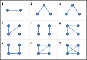
Figure 1: The $9$ connected subgraphs of size less than or equal to $4$.

III.2 Our spectral approach

Our second approach to defining similarities between graphs was initially motivated by the approach given in Vishwanathan et al. (2010), and we based it on the notion of non-conservative diffusion on graphs Ghosh et al. (2011). There are, of course, numerous ways in which spectral information of graphs (or equivalently information from performing random walks on graphs) could be used to define similarity measures. The particular version of the similarity metric discussed here is inspired by the spectral decomposition algorithm in Vishwanathan et al. (2010). The usual definition of random walks on graphs is based on a physical diffusion process. One starts with a given initial density of random walkers, who are then redistributed at every step by premultiplying the distribution of random walkers at the current stage by the graph adjacency matrix. The rows of the adjacency matrix are scaled by the row sum, so that the quantity of random walkers is conserved. In our approach, we consider a non-conservative diffusion process where we replace the normalized adjacency matrix in the random walk process by its original, unnormalized counterpart.

Let us consider graphs $G_{i}$ and $G_{j}$, with adjacency matrices $B_{i}$ and $B_{j}$ respectively. Let their spectral decompositions be given by $B_{i}=P_{i}D_{i}P_{i}^{T}$ and $B_{j}=P_{j}D_{j}P_{j}^{T}$ respectively. Let the initial probability distribution of random walkers on the $n$ nodes of the graph be denoted by $\hat{p}$. This can be taken to be the uniform distribution. At every step of the process, the new distribution of random walkers is found by applying the unnormalized adjacency matrix to the distribution at the previous step. Since the adjacency matrix is not normalized, the density of random walkers changes over time depending on the weights associated with the edges of the graphs. We consider walks of different lengths, at the end of which we evaluate statistics by weighing the density of random walkers on the nodes according to a prescribed vector $\hat{q}$; this can also be assumed to be a uniform vector that takes the value $1/n$ at every node. As pointed out in Vishwanathan et al. (2010), the vectors $\hat{p}$ and $\hat{q}$ are ways to “embed prior knowledge into the kernel design”. We reiterate that, although the method is general, we will consider the special case where the sizes of the graphs are the same.

The (possibly weighted) average density of random walkers after a k-length walk in $G_{i}$, is denoted by $Q_{ik}$. This can be evaluated as follows:

$$Q_{ik}=\hat{q}^{T}B_{i}^{k}\hat{p}=\hat{q}^{T}(P_{i}D_{i}^{k}P_{i}^{T})\hat{p}.$$ (5)

Consider a summation of $Q_{ik}$ for walks of all lengths, with appropriate weights $\mu_{k}$ corresponding to each value of $k$. Let the computed weighted sum of densities corresponding to graph $G_{i}$ be denoted as $S_{i}$.

$$S_{i}=\sum_{k=0}^{\infty}\mu(k)Q_{ik}=\sum_{k=0}^{\infty}\mu(k)~{}l_{i}^{T}D_{i}^{k}r_{i}.$$ (6)

where $l_{i}=P_{i}^{T}\hat{q}$ and $r_{i}=P_{i}^{T}\hat{p}$.

We used the following choice of weighting relation: $\mu(k)=\frac{\lambda^{k}}{k!}$. With this choice of weights, one can write $S_{i}$ as a simple function of $\lambda$ as follows:

$$S_{i}(\lambda)=l_{i}^{T}e^{(\lambda D_{i})}r_{i}.$$ (7)

Thus, every graph $G_{i}$ is embedded using these $S_{i}$ values evaluated at characteristic values of $\lambda$ (say $\lambda_{1},\lambda_{2},...\lambda_{M}$). A similarity between any two graphs $G_{i}$ and $G_{j}$ can then be evaluated using the Gaussian kernel defined in Eq. 4 using the following expression for $k(G_{i},G_{j})$:

$$k(G_{i},G_{j})=\sqrt{\sum_{m=1}^{M}(S_{i}(\lambda_{m})-S_{j}(\lambda_{m}))^{2}}.$$ (8)

This formula is simple and convenient for our purpose. For every graph $G_{i}$, one can evaluate the three vectors, $l_{i}$, diagonal elements of $D_{i}$ and $r_{i}$ and store them. The $3n$ values they are comprised of can be thought of (and used) as a coarse embedding of the graph. The similarity measure between pairs of graphs can then finally be evaluated by using Eq. 7 and Eq. 8 in terms of these stored values. This also makes it straightforward to add new graphs in the ensemble, increasing the size of the similarity matrix without much additional computation.

IV Computational results

We will explore the dimensionality of datasets (where the data points are individual graphs) using the diffusion map approach; within this approach we will construct implementations using the graph similarity metrics mentioned above. We use three different datasets for this exploration; two of them arise in the context of “graph-generation” models (they are the ubiquitous Erdös-Rényi networks and the Chung-Lu networks). The third is closer to the types of applications that motivated our work: networks that arise as individual temporal “snapshots” during a dynamic network evolution problem.

IV.1 Test case $1$: Erdös-Rényi graphs

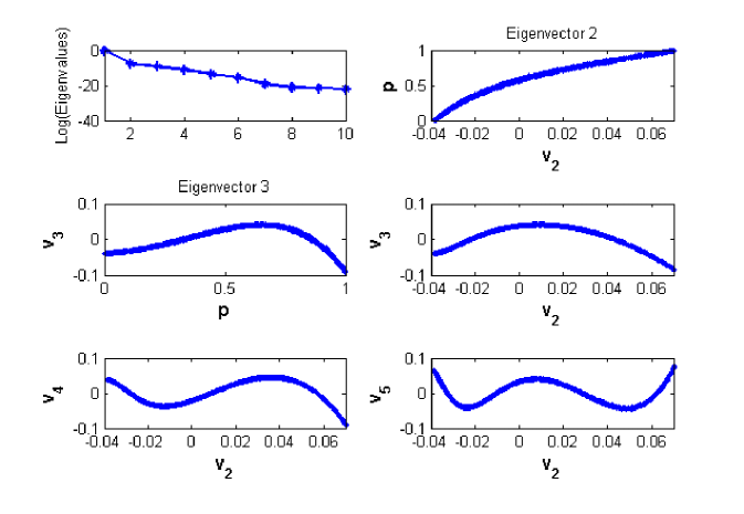
Figure 2: Data mining ensembles of Erdös-Rényi graphs: The subgraph approach was used to quantify similarity between individual graphs. The top-left plot shows the first $10$ eigenvalues of the random walk matrix arising in Diffusion Maps. The corresponding first two non-trivial eigenvectors are plotted against the “construction parameter” $p$ used to create the graphs, as well as against each other. Notice how the first non-trivial eigenvector (the second eigenvector) is one-to-one with $p$. The fourth and fifth eigenvectors are also plotted against the second eigenvector. An $\epsilon$ of 0.5 was used in the diffusion map algorithm.

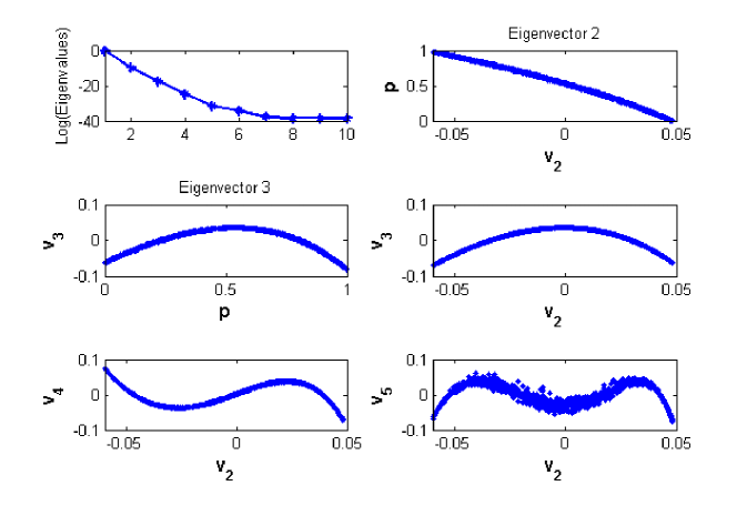
Figure 3: Data mining ensembles of Erdös-Rényi graphs: Our spectral approach was used to quantify similarity between graphs. The top-left plot shows the first $10$ eigenvalues of the random walk matrix arising in Diffusion Maps. The corresponding first two non-trivial eigenvectors are plotted against the construction parameter $p$ used to create the graphs, as well as against each other. Notice how, again, the first non-trivial eigenvector (the second eigenvector) is one-to-one with $p$. The fourth and fifth eigenvectors are also plotted against the second eigenvector. An $\epsilon$ of 5 was used in the diffusion map algorithm.

Consider, as our initial example, a dataset consisting of $m=1000$ Erdös-Rényi $G(n,p)$ random graphs Erdös and Rényi (1959) with $n=100$ nodes each. The parameter $p$ (the probability of edge existence) used to construct these graphs is randomly sampled uniformly in the interval $(0,1)$. We start by computing the similarity measures between pairs of individual graphs (both the subgraph approach (Eq. 3) using $9$ subgraph densities and our spectral approach (Eq. 8 using 100 values of $\lambda$ uniformly spaced from $0.0001$ to $0.01$). The similarity matrix $W$ is then calculated using Eq. 4. The first $10$ eigenvalues of the corresponding random walk matrix $A$, (as described in Sec. II) are plotted in Figs. 2 and 3, corresponding to the subgraph approach and to our spectral approach respectively. For both these cases, the first two non-trivial eigenvectors (viz., the eigenvectors corresponding to the second and third eigenvalues) are plotted against the parameter $p$ of the corresponding Erdös-Rényi graph. From the figures, it is clear that the second eigenvector is one-to-one with the parameter $p$, which here is also the edge-density. Thus, this eigenvector (in both cases) captures the principal direction of variation in the collection of Erdös-Rényi graphs. In other words, our data mining approach independently recovers the single important parameter $p$ in our sample dataset.

In diffusion maps, the first non-trivial eigenvector always characterizes the principal direction in the dataset. Subsequent eigenvectors can represent one of the following: (i) higher harmonics of the principal direction, (ii) new directions in the dataset, or (iii) noise (in this case, the variability of sampling among Erdös-Rényi graphs of the same $p$). One can discriminate between these options by plotting the eigenvectors against each other and looking for correlations. In this example, when subsequent eigenvectors are plotted against the second, we clearly observe that they are simply higher harmonics in its “direction”. The third, fourth and fifth eigenvectors, in both cases, are clearly seen to be a non-monotonic function of $v_{2}$($p$) but with an increasing number of “spatial” oscillations, reminiscent of Sturm-Liouville type problem eigenfunction shapes. These eigenvectors do not, therefore, capture new directions in the space of our sample graphs.

This simple example serves to illustrate the purpose of using data mining algorithms on graph data. In this case, we created a one parameter family of graphs, characterized by the parameter $p$. Using only the resulting graph objects, our data mining approach successfully recovered a characterization of these graphs equivalent to (one-to-one with) this parameter $p$. One feature of this one-to-one correspondence between $p$ and the $v_{2}$ component of the graphs is worth more discussion: data mining discovers the “one-dimensionality” of the data ensemble, but does not explicitly identify $p$ - a parameterization that has a direct and obvious physical meaning. Data mining only provides a parameterization effectively isomorphic to the one by $p$: to the eye the $p$-$v_{2}$ function appears continuous and with a continuous inverse. Providing a physical meaning for the parameterization discovered (or finding a physically meaningful parameterization isomorphic to the one discovered) is a completely separate task, where the modeler has to provide good candidates. The contribution of the data-mining process is determining the number of necessary parameters, and in providing a quantity against which good candidates can be tested.

IV.2 Test case $2$: A two parameter family of graphs

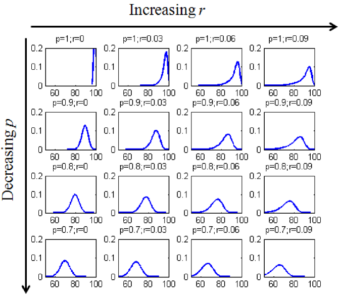
Figure 4: The degree distribution of Chung-Lu graphs created using the algorithm described in the text are plotted for various values of the construction parameters $p$ and $r$. The parameter $p$ corresponds to the density of edges in the graph. As $p$ decreases, the degree distribution shifts uniformly to the left. The parameter $r$ corresponds roughly to the skewness of the degree distribution. As $r$ is increased from $0$, the degree distribution shifts to the left, but the resulting degree distributions are skewed more and more to the left.

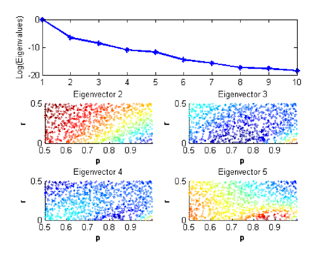
Figure 5: Data mining ensembles of two-parameter Chung-Lu graphs: The leading eigenvalues of the random walk matrix calculated using the subgraph similarity measure are first plotted. The corresponding first four non-trivial eigenvectors are then illustrated in a way that brings forth their relation to the construction parameters $p$ and $r$. In these plots, each graph is denoted as a point. The $x$ and $y$ coordinates of the point correspond to the parameters $p$ and $r$ used to construct that particular graph. The graphs are colored based on the magnitude of their components in the eigenvectors of the random walk matrix $A$. An $\epsilon$ of 10 was used in the diffusion map algorithm.

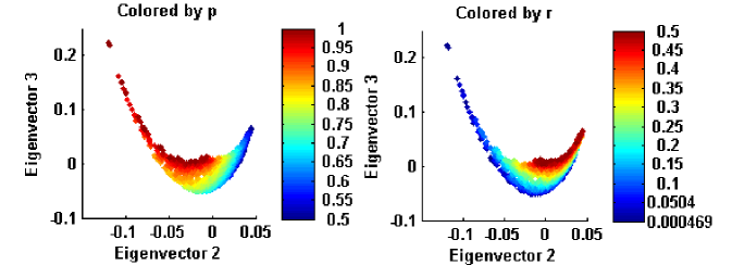
Figure 6: Data mining the two-parameter family of Chung-Lu graphs using the subgraph similarity metric leads to an apparent two-dimensional embedding. In these plots the $x$ and $y$ coordinates of each point (i.e. of each graph in the dataset) denote the components of that particular graph in the second and third eigenvectors of the random walk matrix respectively. Each point is now colored based on the parameter values of $p$ (left) and $r$ (right) used to construct the particular graph.

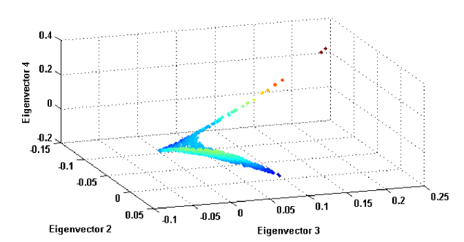
Figure 7: A $3-d$ plot suggesting that the fourth eigenvector of the random walk matrix -calculated using the subgraph similarity measure- for the case of the two parameter family of Chung-Lu graphs can be expressed as a function of the second and third eigenvectors: it does not capture a new direction in the space of our sample graphs.

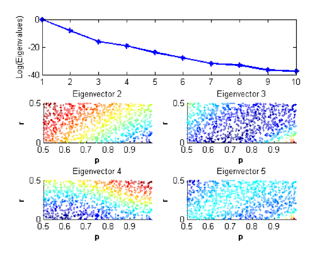
Figure 8: Data mining ensembles of two-parameter Chung-Lu graphs: The leading eigenvalues of the random walk matrix calculated using our spectral similarity measure are first plotted. The corresponding first four non-trivial eigenvectors are then illustrated in a way that brings forth their relation to the construction parameters $p$ and $r$. In these plots, each graph is denoted as a point. The $x$ and $y$ coordinates of the point correspond to the parameters $p$ and $r$ used to construct that particular graph. The graphs are colored based on the magnitude of their components in the eigenvectors of the random walk matrix $A$. An $\epsilon$ of 10 was used in the diffusion map algorithm.

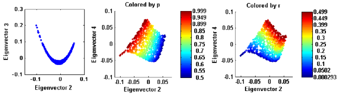
Figure 9: Data mining the two-parameter family of Chung-Lu graphs using the spectral similarity metric leads to an apparent two-dimensional embedding. In these plots the $x$ and $y$ coordinates of each point (i.e. of each graph in the dataset) denote the components of that particular graph in the second and third (resp., fourth) eigenvectors of the random walk matrix for the left plot (resp., middle and right plots). Each point is also colored based on the parameter values of $p$ (middle plot) and $r$ (right plot) used to construct the particular graph. An $\epsilon$ of 10 was used in the diffusion map algorithm.

We now consider a slightly richer dataset, where the graphs are constructed using two independent parameters. The definition of this illustrative family of graphs is based on the Chung-Lu algorithm Chung and Lu (2002). For a graph consisting a $n$ vertices (here $n=100$), following their original algorithm, we begin by assigning a weight $w_{i}$ to each vertex $i,1\leq i\leq n$. The weights we chose have the two-parameter form $w_{i}=np(i/n)^{r}$. The probability $P_{ij}$ of existence of the edge between vertices $i$ and $j$ is given by $P_{ij}=min(B_{ij},1)$, where

$$B_{ij}=\frac{w_{i}w_{j}}{\sum_{k}{w_{k}}}.$$ (9)

Once the edge existence probabilities are calculated, a graph can be constructed by sampling uniform random numbers between $0$ and $1$ for every pair of vertices $(i,j)$ and placing an edge between them if the random number is less than $P_{ij}$. Note that in the original Chung-Lu algorithm $P_{ij}=B_{ij}$. If the weights are chosen such that $B_{ij}\leq 1,\forall(i,j)$, then the expected value of the degree of node $i$ will be equal to the chosen weight values $w_{i}$. If any $B_{ij}$ exceeds the value of $1$, this would no longer be the case Chung and Lu (2002).

The model selected here has $2$ construction parameters: $p$ and $r$. If $r=0$, the resulting graphs are Erdös-Rényi graphs and the parameter $p$ represents the edge density. When $p=1$ and $r=0$, the resulting graphs are complete. As $r$ is increased, this procedure creates graphs whose degree distributions are skewed to the left (long tails towards lower degrees). Degree distributions resulting from creating graphs with various combinations of parameters $p$ and $r$ are shown in Fig. 4.

For our illustration, $1000$ graphs were created using this model with $n=100$ nodes each. The values of $p$ and $r$ were chosen by uniformly sampling in the interval $(0.5,1)$ and $(0,0.5)$ respectively. The diffusion maps algorithm was used on this set of graphs exactly as described in the first case. As we will discuss below, the results obtained using the two similarity measures that we consider in this paper, while conveying essentially the same qualitative information, have visible quantitative differences.

The first $10$ eigenvalues of the random walk matrix calculated using the subgraph approach for evaluating similarities are shown in the top plot of Fig. 5. The first four non-trivial eigenvectors are plotted below. In these plots, each of the $1000$ graphs is represented as a point in the $p-r$ two parameter plane. The colors represent the magnitude of the components of the corresponding graph data on each of the first $4$ non-trivial eigenvectors. The gradient of colors in these plots suggest the “direction” of each of these eigenvectors in the $p-r$ plane. However, a more careful inspection of the plots is required to determine independent subsets of these eigenvectors. To help explore this, we plot eigenvectors $2$ and $3$ against each other in Fig. 6. The figure clearly suggests (through its obvious two-dimensionality) that these two eigenvectors are independent of each other. Furthermore, when the points in these plots are colored by the two parameters $p$ and $r$ used to construct the graphs, two independent directions, a roughly “left-to-right” for $p$ and a roughly “top-to-bottom” for $r$, can be discerned on the $v_{2}-v_{3}$ manifold, Fig. 6. This strongly suggests that the Jacobian of the transformation from $(p,r)$ to $(v_{2},v_{3})$ is nonsingular on our data. Thus, these two eigenvectors, obtained solely through our data mining approach, can equivalently be used to parameterize the set of graphs constructed using the parameters $p$ and $r$. The components of the fourth eigenvector plotted in terms of these two leading eigenvectors in Fig. 7 are strong evidence that this fourth eigenvector is completely determined by (is a function of) the second and third ones. In other words, the fourth eigenvector “lives in the manifold” created by the second and third eigenvectors, and hence does not convey more information about (does not parameterize new directions in) our graph dataset.

We now focus on similar results obtained with the same dataset, but now using our spectral approach for measuring similarity. The eigenvalues and eigenvectors of the random walk matrix obtained by this approach are reported in Fig. 8. As before, we plot the leading eigenvectors against each other in Fig. 9. The plot of eigenvector $2$ versus eigenvector $3$ appears as a smooth “almost” curve, suggesting a strong correlation, while the plot of eigenvector $3$ versus eigenvector $4$ clearly shows two-dimensionality. These figures suggest that eigenvectors $2$ and $3$ parameterize the same direction in the $p-r$ plane, while eigenvector $4$ parameterizes a second, new direction in this plane. Hence, eigenvectors $2$ and $4$ constitute independent directions in the space of our sample graphs.

Once again, we have recovered (through data mining) two independent directions in our sample family of graphs that were originally constructed using two independent parameters. Although the results obtained using the subgraph and the spectral approaches in this case are quantitatively different in their details, they are both successful in recovering two independent coordinates in the space of graphs, apparently isomorphic to those given as input to the data mining algorithm. The $2D$ manifold resulting from the subgraph approach appears better at visually capturing the behavior of the original $p-r$ plane. The “quality” of these parameterizations will clearly be affected by the details used in the data-mining procedure and, in particular, those affecting the similarity measure evaluation: the number of subgraph densities kept, the choices for numerical constants such as $\lambda_{i}$ in the subgraph approach, $\epsilon$ in diffusion maps, etc. An obvious criterion in the selection of these method parameters is to make the Jacobian of the transformation from the “natural” to the “data-mining-based” parameterizations as far from singular as possible.

IV.3 Test case $3$: Graphs from a dynamic graph evolution model

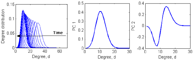
Figure 10: The evolution of degree distribution over time from a single initial condition is shown on the left. The first two principal components (obtained through PCA) of degree sequences, collected from transients starting from different initial conditions are shown on the right.

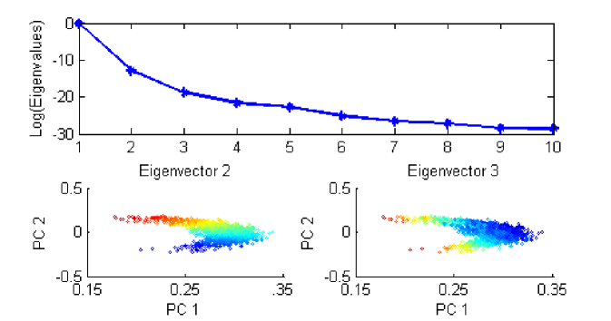
Figure 11: Data mining results for graphs collected from the dynamic graph evolution model: The leading eigenvalues of the random walk matrix calculated using the subgraph similarity measure are plotted. The corresponding first two non-trivial eigenvectors also are shown. In these plots, each graph datum is denoted as a point. The $x$ and $y$ coordinates of the point correspond to the parameters PC $1$ and PC $2$ described in the text. The graphs are colored based on the magnitude of their components in the two leading eigenvectors of the random walk matrix $A$. An $\epsilon$ of 10 was used in the diffusion map algorithm.

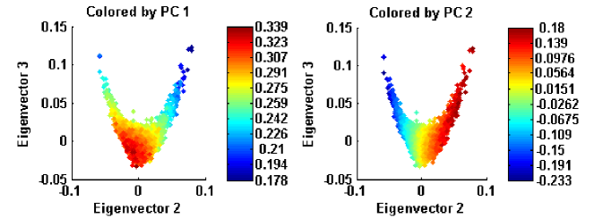
Figure 12: The graph data collected from the dynamic model transients are alternatively plotted in the embedding plane of the two leading diffusion map eigenvectors shown in Fig. 11. The points corresponding to the different graphs are colored based on the component of their degree distributions on the first two degree-distribution principal components.

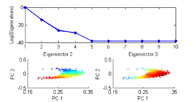
Figure 13: Data mining results for graphs collected from the dynamic graph evolution model: The leading eigenvalues of the random walk matrix calculated using our spectral similarity measure are plotted. The corresponding first two non-trivial eigenvectors also are shown. In these plots, each graph datum is denoted as a point. The $x$ and $y$ coordinates of the point correspond to the parameters PC $1$ and PC $2$ described in the text. The graphs are colored based on the magnitude of their components in the two leading eigenvectors of the random walk matrix $A$. An $\epsilon$ of 50 was used in the diffusion map algorithm.

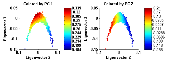
Figure 14: The graph data collected from the dynamic model transients are alternatively plotted in the embedding plane of the two leading diffusion map eigenvectors shown in Fig. 13. The points corresponding to the different graphs are colored based on the component of their degree distributions on the first two degree-distribution principal components.

In the two examples given above, the dataset graphs were created using prescribed rules of a graph-generation model characterized by one or more model parameters. We now consider a case where the graph dataset comes from sampling snaphots of a dynamic process that involves the evolution of graphs. The process sampled could be one occurring in nature/society (for instance, evolution of a social network) or one arising from a dynamic model with prescribed (deterministic or even stochastic) evolution rules. We consider the latter case for illustration, exploiting a simple model of a random evolution of networks Bold et al. (2012); our process is sampled at regular time intervals. A brief description of the model is as follows: Starting from an initial graph, the model rules update the graph structure at every time step by repeatedly sequentially applying the following two operations:

1. A pair of nodes selected at random are connected by an edge if they are not already connected to each other.

2. An edge chosen uniformly at random is removed with probability $r$ (here, $r=0.1$).

The details of the model behavior are discussed in Bold et al. (2012). Here, we will focus only on those characteristics of the model evolution necessary to rationalize the results of data mining. For this particular graph model, it is known that the (expected) degree distribution evolves smoothly in time as shown in the left plot of Fig. 10. Furthermore, it is also known that the evolution of degrees is decoupled from (and occurs at slower time scales than) the evolution of all higher order properties of the graph such as triangles, degree-degree correlations etc. Thus, as argued in Bold et al. (2012), the dynamic evolution of graphs according to this model can be usefully described in terms of degrees or degree distributions only. The temporal evolution starting from several different initial graphs was recorded, and a principal component analysis of a collection of snapshots of degree sequences that arose during these simulations was performed. The two leading principal components are plotted in Fig. 10. The first principal component (PCA), labeled PC $1$, is, in effect, the steady state degree distribution while the second principal component PC $2$ is the direction along which the degree distribution decays the slowest towards stationarity. Since it has been claimed that the degree distribution is the most significant observable in this model, PC $1$ and PC $2$ constitute good variables through which one can track the evolution of the graphs over time. In fact, as shown in Bold et al. (2012), one can write explicit Fokker-Planck equations for the evolution of the distribution of (appropriately shifted and scaled) degrees. The eigenfunctions of the corresponding eigenvalue problem are Hermite polynomials, the first two of which have the qualitative forms, $exp(-x^{2})$ and $x.exp(-x^{2})$; this functional dependence is clearly noticeable in $PC1$ and $PC2$ respectively.

We now ignore our knowledge of explicit models of the dynamical process, and focus on the sampled graph sequences created by the process. Our goal is to use diffusion maps to discover -using only the graph snapshot data- good variables through which to characterize the data. These variables should then also be useful in describing the dynamics of the evolution process – we anticipate that the data-mining variables and the variables PC $1$ and PC $2$ would embody similar information about the process. As before, we use both the subgraph and our spectral similarity measures. The eigenvalues and the first two non-trivial eigenvectors of the random walk matrix in diffusion maps are shown for each similarity measure in Figs. 11 and 13 respectively. The plots are constructed so that the plotted points (each corresponding to a sampled graph) lie in the plane of the principal components PC $1$ and PC $2$; the points are colored by the corresponding eigenvector components, for comparison. In both cases, the results show that the second and third eigenvectors have the most variation (as indicated by the gradient of colors) in the directions of PC $2$ and PC $1$ resp. This suggests that the first two non-trivial eigenvectors are roughly one-to-one with PC $2$ and PC $1$ respectively. Conversely, we can plot the graphs in the space of the diffusion map eigenvectors (the new embedding) and color them based on PC $1$ and PC $2$ as shown in Figs. 12 and 14 (one for each of our similarity measures). These two figures convey again the one-to-one nature of the transformation between Principal Component based and diffusion map based parameterization of the dynamic graph evolution data - yet the diffusion map based parameterization did not use prior knowledge about significant observables of the process. In the example considered here, the fact that theoretical results were available was used to validate our data mining, providing a reference with which to compare. The implication is that, even in problems where such theoretical results are not available, data mining can be used to gain an understanding about the primary driving factors in the dynamics of the system - provided that a relatively small number of such factors can be used to effectively model the process.

V Conclusions

We studied the problem of data mining in cases where the data points occur in the form of graphs. The main obstacle in applying established data mining algorithms to such cases is the definition of good measures quantifying the similarity between pairs of graphs. We discussed two common sense approaches to tackle this problem: the subgraph method, which compares the local structures in the graphs, and a spectral method, which is based on defining diffusion processes on the graphs. While alternate definitions of similarity metrics than the ones discussed in this paper are eminently possible, and probably very useful, the purpose of this paper is to demonstrate the usefulness of data mining in the context of graph data using a few illustrative examples for which the parameterizations obtained through our approach could be compared with known results. Certain remarks regarding the similarity measures used in this paper should however be made. The subgraph approach to evaluate similarity is much more computationally expensive, compared to our spectral approach, especially when larger sized subgraphs must be included to get useful results. (For example, there are $6$ connected subgraphs of size $4$, while there are $21$ subgraphs of size $5$. Searching for larger subgraphs becomes computationally increasingly more expensive). Both approaches require us to tune certain method parameters associated with the definitions of the similarity metric and the data mining approach. For the diffusion map algorithm, one has to choose a suitable size of neighborhood ($\epsilon$). In addition, the spectral approach requires one to define the weighting function, $\mu(k)$ (and also make assumptions about the vectors $p$ and $q$). This can be thought as analogous to selecting suitable normalizations in defining the subgraph densities in the subgraph approach. Such tuning considerations become especially crucial when one is confronted with data from a completely new problem, where intuition cannot be used to guide the selection of model parameters. Considering the trade-offs mentioned above, it might be reasonable to use the subgraph density approach to find similarities between graphs initially for new problems, and to subsequently “tune” spectral decomposition algorithm, which can then be used for faster computations.

We used three sample sets of graph data in this work. The first example was a collection of Erdös-Rényi random graphs with varying parameters. We also considered the case of graphs obtained from a simple two-parameter family of graphs motivated by the Chung-Lu algorithm. Both examples considered graphs created from a fixed model. As a third example, we used a collection of graphs from a dynamic model. In all these examples, we used the data mining approach with two different approaches for measuring similarities to extract good characterizations of the graph datasets with identical size graphs, and compared them to known parameterizations. A weighted version of the graph size can be used as part of the selected similarity measure; so that the measures we used can be extended to datasets with varying graph sizes.

An important motivation for our work is the desire to use the data mining-induced observables as variables in the equation-free modeling of graph evolution (Kevrekidis et al. (2003, 2004), see Bold et al. (2012); Tsoumanis et al. (2012) for graph-related applications). Even if explicit models for the coarse-grained evolution of graphs may not be available/easy to derive, the idea is that one can still use well-designed brief bursts of detailed network evolution simulations to effectively perform coarse-scale computations. In this process -and the associated algorithms, like coarse projective integration- the ability to fluently translate from fine (detailed network) to coarse-grained (reduced, only important statistics) descriptions lies at the heart of the approach. Several good attempts for implementing the reverse step of this transformation (lifting from coarse statistics to detailed networks consistent with them) can be found in the literature Havel (1955); Dorogovtsev et al. (2002); Holme and Kim (2002); Serrano and Boguná (2005); Gounaris et al. (2011); using data-mining inspired observables in such equation-free coarse-graining is a significant challenge, one that we are currently exploring.