Symbolic-numerical Algorithm for Generating
Cluster Eigenfunctions: Tunneling of Clusters Through Repulsive Barriers

Abstract

A model for quantum tunnelling of a cluster comprising $A$ identical particles, coupled by oscillator-type potential, through short-range repulsive potential barriers is introduced for the first time in the new symmetrized-coordinate representation and studied within the s-wave approximation. The symbolic-numerical algorithms for calculating the effective potentials of the close-coupling equations in terms of the cluster wave functions and the energy of the barrier quasistationary states are formulated and implemented using the Maple computer algebra system. The effect of quantum transparency, manifesting itself in nonmonotonic resonance-type dependence of the transmission coefficient upon the energy of the particles, the number of the particles $A=2,3,4$, and their symmetry type, is analyzed. It is shown that the resonance behavior of the total transmission coefficient is due to the existence of barrier quasistationary states imbedded in the continuum. .

1 Introduction

During a decade, the mechanism of quantum penetration of two bound particles through repulsive barriers [1] attracts attention from both theoretical and experimental viewpoints in relation with such problems as near-surface quantum diffusion of molecules  [2, 3, 4], fragmentation in producing very neutron-rich light nuclei  [5, 6], and heavy ion collisions through multidimensional barriers [7, 8, 9, 10, 11, 12, 13, 14]. Within the general formulation of the scattering problem for ions having different masses, a benchmark model with long-range potentials was proposed in Refs. [15, 16, 17]. The generalization of the two-particle model over a quantum system of $A$ identical particles is of great importance for the appropriate description of molecular and heavy-ion collisions. The aim of this paper is to present the convenient formulation of the problem stated above and the calculation methods, algorithms, and programs for solving this problem.

We consider a new method for the description of the penetration of $A$ identical quantum particles, coupled by short-range oscillator-like interaction, through a repulsive potential barrier. We assume that the spin part of the wave function is known, so that only the spatial part of the wave function is to be considered, which may be symmetric or antisymmetric with respect to a permutation of $A$ identical particles. The initial problem is reduced to the penetration of a composite system with the internal degrees of freedom, describing an $(A-1)\times d$-dimensional oscillator, and the external degrees of freedom describing the center-of-mass motion of $A$ particles in $d$-dimensional Euclidian space. For simplicity, we restrict our consideration to the so-called $s$-wave approximation [1] corresponding to one-dimensional Euclidean space ($d=1$).

We seek for the solution in the form of Galerkin expansion in terms of cluster functions in the new symmetrized coordinate representation (SCR) [18] with unknown coefficients having the form of matrix functions of the center-of-mass variable. As a result, the problem is reduced to a boundary-value problem for a system of ordinary second-order differential equations with respect to the center-of-mass variable. Conventional asymptotic boundary conditions involving unknown amplitudes of reflected and transmitted waves are imposed on the desired matrix solution. Solving the problem was implemented as a complex of the symbolic-numeric algorithms and programs in CAS MAPLE and FORTRAN environment. The results of calculations are analyzed with particular emphasis on the effect of quantum transparency that manifests itself as nonmonotonic energy dependence of the transmission coefficient due to resonance tunnelling of the bound particles in S (A) states through the repulsive potential barriers.

The paper is organized as follows. In Section 2, we present the problem statement in symmetrized coordinates. In Section 3, we introduce the SCR of the cluster functions of the considered problem and the asymptotic boundary conditions involving unknown amplitudes of reflected and transmitted waves. In Section 4, we formulate the boundary-value problem for the close-coupling equations in the Galerkin form using the SCR. In Section 5, we analyze the results of numerical experiment on the resonance transmission of a few coupled identical particles in S(A) states, whose energies coincide with the resonance eigenenergies of the barrier quasi-stationary states embedded in the continuum. In Conclusion, we sum up the results and discuss briefly the perspectives of application of the developed approach.

2 Problem Statement

We consider a system of $A$ identical quantum particles having the mass $m$ and a set of the Cartesian coordinates $x_{i}\in{\bf R}^{d}$ in $d$-dimensional Euclidian space, considered as vector $\tilde{\bf x}=(\tilde{x}_{1},...,\tilde{x}_{A})\in{\bf R}^{A\times d}$ in $A\times d$-dimensional configuration space. The particles are coupled by the pair potentials $\tilde{V}^{pair}(\tilde{x}_{ij})$ depending upon the relative coordinates, $\tilde{x}_{ij}=\tilde{x}_{i}-\tilde{x}_{j}$, similar to a harmonic oscillator potential $\tilde{V}^{hosc}(\tilde{x}_{ij})=\frac{m\omega^{2}}{2}(\tilde{x}_{ij})^{2}$ with the frequency $\omega$. The resulting clusters are subject to the influence of the potentials $\tilde{V}(\tilde{x}_{i})$ describing the external field of a target. The appropriate Schrödinger equation takes the form

$$\left[\!-\!\frac{\hbar^{2}}{2m}\sum_{i=1}^{A}\frac{\partial^{2}}{\partial\tilde{x}_{i}^{2}}\!+\!\sum_{i,j=1;i<j}^{A}\tilde{V}^{pair}(\tilde{x}_{ij})\!+\!\sum_{i=1}^{A}\tilde{V}(\tilde{x}_{i})\!-\!\tilde{E}\right]\tilde{\Psi}(\tilde{\bf x})\!=\!0,$$

where $\tilde{E}$ is the total energy of the system of $A$ particles, and $\tilde{P}^{2}={2m\tilde{E}}/{\hbar^{2}}$, $\tilde{P}$ is the total momentum of the system, and $\hbar$ is Planck constant. Using the oscillator units $x_{osc}=\sqrt{\hbar/(m\omega\sqrt{A})}$, $p_{osc}=\sqrt{(m\omega\sqrt{A})/\hbar}=x_{osc}^{-1}$, and $E_{osc}=\hbar\omega\sqrt{A}/2$ to introduce the dimensionless coordinates $x_{i}=\tilde{x}_{i}/x_{osc}$, $x_{ij}=\tilde{x}_{ij}/x_{osc}=x_{i}-x_{j}$, $E=\tilde{E}/E_{osc}=P^{2}$, $P=\tilde{P}/p_{osc}=\tilde{P}x_{osc}$, $V^{pair}(x_{ij})=\tilde{V}^{pair}(x_{ij}x_{osc})/E_{osc}$, $V^{hosc}(x_{ij})=\tilde{V}^{hosc}(x_{ij}x_{osc})/E_{osc}=\frac{1}{A}(x_{ij})^{2}$ and $V(x_{i})=\tilde{V}(x_{i}x_{osc})/E_{osc}$, one can rewrite the above equation in the form

$$\left[\!-\!\sum_{i=1}^{A}\frac{\partial^{2}}{\partial x_{i}^{2}}\!+\!\!\sum_{i,j=1;i<j}^{A}\frac{1}{A}(x_{ij})^{2}\!+\!\!\sum_{i,j=1;i<j}^{A}\!U^{pair}(x_{ij})\!+\!\!\sum_{i=1}^{A}V(x_{i})\!-\!E\right]\Psi({\bf x})\!=\!0,$$ (1)

where $U^{pair}(x_{ij})=V^{pair}(x_{ij})-V^{hosc}(x_{ij})$, i.e., if $V^{pair}(x_{ij})=V^{hosc}(x_{ij})$, then $U^{pair}(x_{ij})=0$.

The problem of tunnelling of a cluster of $A$ identical particles in the symmetrized coordinates $(\xi_{0},{\mbox{\boldmath$\xi$}})$, where ${\mbox{\boldmath$\xi$}}=\{\xi_{1},...,\xi_{A-1}\}$:

$$\!\!\xi_{0}=\frac{1}{\sqrt{A}}\left(\sum_{t=1}^{A}x_{t}\right),\,\,\xi_{s}=\frac{1}{\sqrt{A}}\left(x_{1}+\!\!\sum_{t=2}^{A}a_{0}x_{t}+\sqrt{A}x_{s+1}\right),\,\,s=1,...,A-1,$$ (2)

in terms of total potential $U(\xi_{0},{\mbox{\boldmath$\xi$}})=V(\xi_{0},{\mbox{\boldmath$\xi$}})+U^{eff}(\xi_{0},{\mbox{\boldmath$\xi$}})$ reads as [18]

$$\left[-\frac{\partial^{2}}{\partial\xi_{0}^{2}}+\sum_{i=1}^{A-1}\left(-\frac{\partial^{2}}{\partial\xi_{i}^{2}}+(\xi_{i})^{2}\right)+U(\xi_{0},{\mbox{\boldmath$\xi$}})-E\right]\Psi(\xi_{0},{\mbox{\boldmath$\xi$}})=0,$$ (3)

$$U^{eff}(\xi_{0},{\mbox{\boldmath$\xi$}})=\sum_{i,j=1;i<j}^{A}U^{pair}(x_{ij}({\mbox{\boldmath$\xi$}})),\quad V(\xi_{0},{\mbox{\boldmath$\xi$}})=\sum_{i=1}^{A}V(x_{i}(\xi_{0},{\mbox{\boldmath$\xi$}})),$$

which is invariant under permutations $\xi_{i}\leftrightarrow\xi_{j}$ at $i,j=1,...,A-1$, i.e., the invariance of Eq. (1) under permutations $x_{i}\leftrightarrow x_{j}$ at $i,j=1,...,A$ survives the transformation.

3 Cluster Functions and Asymptotic Boundary Conditions

For simplicity we restrict our consideration to the so-called $s$-wave approximation [1], i.e., one-dimensional Euclidian space ($d=1$). Cluster functions $\tilde{\Phi}_{j}(\xi_{0},{\mbox{\boldmath$\xi$}}),$ where ${\mbox{\boldmath$\xi$}}=\{\xi_{1},...,\xi_{A-1}\},$ corresponding to the threshold energies $\tilde{\epsilon}_{j}(\xi_{0})$ dependent on $\xi_{0}$ as a parameter, are solutions of the parametric eigenvalue problem

$$\left(-\frac{\partial^{2}}{\partial{\mbox{\boldmath$\xi$}}^{2}}+{\mbox{\boldmath$\xi$}}^{2}+U(\xi_{0},{\mbox{\boldmath$\xi$}})-\tilde{\epsilon}_{j}(\xi_{0})\right)\tilde{\Phi}_{j}(\xi_{0},{\mbox{\boldmath$\xi$}})=0,\int_{-\infty}^{+\infty}\!\!\!\!\!\!\tilde{\Phi}_{i}(\xi_{0},{\mbox{\boldmath$\xi$}})\tilde{\Phi}_{j}(\xi_{0},{\mbox{\boldmath$\xi$}})d^{A-1}{\mbox{\boldmath$\xi$}}=\delta_{ij},$$ (4)

where $U(\xi_{0},{\mbox{\boldmath$\xi$}})=V(\xi_{0},{\mbox{\boldmath$\xi$}})+U^{eff}(\xi_{0},{\mbox{\boldmath$\xi$}})$ is the total potential that enters Eq. (3). The effective potential $U^{eff}(\xi_{0},{\mbox{\boldmath$\xi$}})$ can be approximated also by the deformed Wood–Saxon potential in the single-particle oscillator approximation [9]. We seek for the cluster functions $\Phi_{i}(\xi_{0},{\mbox{\boldmath$\xi$}})$ in the form of an expansion over the eigenfunctions $\Phi_{j^{\prime}}^{S(A)}(\mbox{\boldmath$\xi$})$, symmetric (S) or antisymmetric (A) with respect to a permutation of the initial $A$ Cartesian coordinates of $A$ identical particles. These functions correspond to eigenenergies $E^{S(A)}_{i}$ of the $(A-1)$-dimensional oscillator, generated by the algorithm SCR [18], with unknown coefficients $\tilde{\alpha}^{(i)}_{j^{\prime}}(\xi_{0})$:

$$\tilde{\Phi}_{i}(\xi_{0},\mbox{\boldmath$\xi$})=\sum_{j^{\prime}=1}^{j^{\prime}_{\max}}\tilde{\alpha}^{(i)}_{j^{\prime}}(\xi_{0})\Phi^{S(A)}_{j^{\prime}}(\mbox{\boldmath$\xi$}).$$ (5)

Thus, the eigenvalue problem (4) is reduced to a linearized version of the Hartree–Fock algebraic eigenvalue problem

$$\sum_{j^{\prime}=1}^{j^{\prime}_{\max}}\left(\delta_{ij^{\prime}}E_{i}^{S(A)}+U_{ij^{\prime}}(\xi_{0})-\delta_{ij^{\prime}}\tilde{\epsilon}_{i}(\xi_{0})\right)\tilde{\alpha}^{(i)}_{j^{\prime}}(\xi_{0})=0,~{}~{}\sum_{j^{\prime}=1}^{j^{\prime}_{\max}}\tilde{\alpha}^{(i^{\prime})}_{j^{\prime}}(\xi_{0})\tilde{\alpha}^{(i)}_{j^{\prime}}(\xi_{0})=\delta_{ii^{\prime}},$$ (6)

where the potentials $U^{pair}_{ij^{\prime}}$ and $V_{ij^{\prime}}(\xi_{0})$ are expressed in terms of the integrals

$$U^{pair}_{ij^{\prime}}=\int d^{A-1}\mbox{\boldmath$\xi$}\Phi_{i}^{S(A)}(\mbox{\boldmath$\xi$})U^{eff}({\mbox{\boldmath$\xi$}})\Phi_{j^{\prime}}^{S(A)}(\mbox{\boldmath$\xi$}),$$ (7)

$$V_{ij^{\prime}}(\xi_{0})=\int d^{A-1}\mbox{\boldmath$\xi$}\Phi_{i}^{S(A)}(\mbox{\boldmath$\xi$})\left(\sum_{k=1}^{A}V(x_{k}(\xi_{0},\mbox{\boldmath$\xi$}))\right)\Phi_{j^{\prime}}^{S(A)}(\mbox{\boldmath$\xi$}).$$ (8)

The parametric algorithm SCR, i.e., algorithm PSCR, for solving the above parametric eigenvalue problem was implemented by means of subroutines [19, 20], or in the single-particle approximation by means of the subroutine [9] in CAS MAPLE and FORTRAN environment.
(G) If $U_{ij^{\prime}}(\xi_{0})=U^{pair}_{ij^{\prime}}$ are independent on $\xi_{0}$, then $\tilde{\epsilon}_{i}(\xi_{0})=\tilde{\epsilon}_{i}$ and $\tilde{\alpha}^{(i)}_{j^{\prime}}(\xi_{0})=\tilde{\alpha}^{(i)}_{j^{\prime}}$ are also independent of $\xi_{0}$, and (5) reduces to $\tilde{\Phi}_{i}(\mbox{\boldmath$\xi$})=\sum_{j^{\prime}=1}^{j^{\prime}_{\max}}\tilde{\alpha}^{(i)}_{j^{\prime}}\Phi^{S(A)}_{j^{\prime}}(\mbox{\boldmath$\xi$})$.
(O) If $V^{pair}(x_{ij})=V^{hosc}(x_{ij})$ and $U^{pair}_{ij^{\prime}}=0$, then $\tilde{\epsilon}_{i}=E^{S(A)}_{i}$ and $\tilde{\alpha}^{(i)}_{j^{\prime}}=\delta_{ij^{\prime}}$.

For the short-range barrier potentials $V(\xi_{0},x_{i}({\mbox{\boldmath$\xi$}}))$ in terms of the asymptotic cluster functions $\tilde{\Phi}_{j}({\mbox{\boldmath$\xi$}})\rightarrow\tilde{\Phi}_{j}(\xi_{0},{\mbox{\boldmath$\xi$}})$ at $|\xi_{0}|\rightarrow\infty$ the asymptotic boundary conditions for the solution $\Psi(\xi_{0},{\mbox{\boldmath$\xi$}})=\{\Psi_{i_{o}}(\xi_{0},{\mbox{\boldmath$\xi$}})\}_{i_{o}=1}^{N_{o}}$ in the asymptotic region $|{\mbox{\boldmath$\xi$}}|/|\xi_{0}|\ll 1$ have the form [16]

$$\Psi_{i_{o}}^{\stackrel{{\scriptstyle\scriptstyle\leftarrow}}{{\scriptstyle\to}}}(\xi_{0}\to\pm\infty,{\mbox{\boldmath$\xi$}})\rightarrow\tilde{\Phi}_{i_{o}}({\mbox{\boldmath$\xi$}})\frac{\exp\left(\mp\imath\left(p_{i_{o}}\xi_{0}\right)\right)}{\sqrt{p_{i_{o}}}}+\sum_{j=1}^{N_{o}}\tilde{\Phi}_{j}({\mbox{\boldmath$\xi$}})\frac{\exp\left(\pm\imath\left(p_{j}\xi_{0}\right)\right)}{\sqrt{p_{j}}}R_{ji_{o}}^{\stackrel{{\scriptstyle\scriptstyle\leftarrow}}{{\scriptstyle\to}}}(E),$$

$$\Psi_{i_{o}}^{\stackrel{{\scriptstyle\scriptstyle\leftarrow}}{{\scriptstyle\to}}}(\xi_{0}\to\mp\infty,{\mbox{\boldmath$\xi$}})\rightarrow\sum_{j=1}^{N_{o}}\tilde{\Phi}_{j}({\mbox{\boldmath$\xi$}})\frac{\exp\left(\mp\imath\left(p_{j}\xi_{0}\right)\right)}{\sqrt{p_{j}}}T_{ji_{o}}^{\stackrel{{\scriptstyle\scriptstyle\leftarrow}}{{\scriptstyle\to}}}(E),$$ (9)

$$\Psi_{i_{o}}^{\stackrel{{\scriptstyle\scriptstyle\leftarrow}}{{\scriptstyle\to}}}(\xi_{0},|{\mbox{\boldmath$\xi$}}|\to\infty)\rightarrow 0.$$

Here $v=\leftarrow,\rightarrow$ indicates the initial direction of the particle motion along the $\xi_{0}$ axis, $N_{o}$ is the number of open channels at the fixed energy $E$ and momentum $p^{2}_{i_{o}}=E-E_{i_{o}}>0$ of cluster; $R_{ji_{o}}^{\leftarrow}=R_{ji_{o}}^{\leftarrow}(E)$, $R_{ji_{o}}^{\rightarrow}=R_{ji_{o}}^{\rightarrow}(E)$ and $T_{ji_{o}}^{\leftarrow}=T_{ji_{o}}^{\leftarrow}(E)$, $T_{ji_{o}}^{\rightarrow}=T_{ji_{o}}^{\rightarrow}(E)$ are the unknown amplitudes of the reflected and transmitted waves. We can rewrite Eqs. (9) in the matrix form $\mbox{\boldmath$\Psi$}=\mbox{\boldmath$\tilde{\Phi}$}^{T}\mbox{\boldmath$F$}$ describing the incident wave and the outgoing waves at $\xi_{0}^{+}\to+\infty$ and $\xi_{0}^{-}\to-\infty$ as

$$\left(\begin{array}[]{ll}\mbox{\boldmath$F$}_{\rightarrow}(\xi_{0}^{+})&\mbox{\boldmath$F$}_{\leftarrow}(\xi_{0}^{+})\\ \mbox{\boldmath$F$}_{\rightarrow}(\xi_{0}^{-})&\mbox{\boldmath$F$}_{\leftarrow}(\xi_{0}^{-})\end{array}\right)\!=\!\left(\begin{array}[]{ll}\mathbf{0}&\mathbf{X}^{(-)}(\xi_{0}^{+})\\ \mathbf{X}^{(+)}(\xi_{0}^{-})&\mathbf{0}\end{array}\right)\!+\!\left(\begin{array}[]{ll}\mathbf{0}&\mathbf{X}^{(+)}(\xi_{0}^{+})\\ \mathbf{X}^{(-)}(\xi_{0}^{-})&\mathbf{0}\end{array}\right)\mathbf{S}.$$ (16)

Here the unitary and symmetric scattering matrix $\mathbf{S}$

$$\mathbf{S}=\left(\begin{array}[]{ll}\mathbf{R}_{\rightarrow}&\mathbf{T}_{\leftarrow}\\ \mathbf{T}_{\rightarrow}&\mathbf{R}_{\leftarrow}\end{array}\right),\quad\mathbf{S}^{\dagger}\mathbf{S}=\mathbf{S}\mathbf{S}^{\dagger}=\mathbf{I},$$ (19)

where $\mathbf{S}^{\dagger}$ is the conjugate transpose of $\mathbf{S}$. It is composed of the matrices, whose elements are reflection and transmission amplitudes that enter Eqs. (9) and possess the following properties[16, 17]:

$$\mathbf{T}_{\rightarrow}^{{\dagger}}\mathbf{T}_{\rightarrow}+\mathbf{R}_{\rightarrow}^{{\dagger}}\mathbf{R}_{\rightarrow}=\mathbf{I}_{oo}=\mathbf{T}_{\leftarrow}^{{\dagger}}\mathbf{T}_{\leftarrow}+\mathbf{R}_{\leftarrow}^{{\dagger}}\mathbf{R}_{\leftarrow},$$

$$\mathbf{T}_{\rightarrow}^{{\dagger}}\mathbf{R}_{\leftarrow}+\mathbf{R}_{\rightarrow}^{{\dagger}}\mathbf{T}_{\leftarrow}=\mathbf{0}=\mathbf{R}_{\leftarrow}^{{\dagger}}\mathbf{T}_{\rightarrow}+\mathbf{T}_{\leftarrow}^{{\dagger}}\mathbf{R}_{\rightarrow},$$ (20)

$$\mathbf{T}_{\rightarrow}^{T}=\mathbf{T}_{\leftarrow},\quad\mathbf{R}_{\rightarrow}^{T}=\mathbf{R}_{\rightarrow},\quad\mathbf{R}_{\leftarrow}^{T}=\mathbf{R}_{\leftarrow}.$$

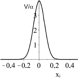
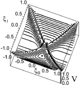
Figure 1: The Gaussian-type potential (24) at $\sigma=0.1$ (in oscillator units) and the corresponding 2D barrier potential at $\alpha=1/10$, $\sigma=0.1$

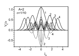
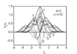
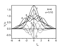
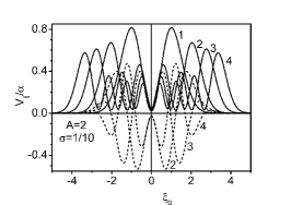
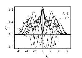
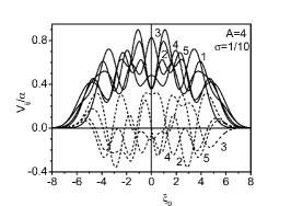
Figure 2: Diagonal $V_{jj}$ (solid lines) and nondiagonal $V_{j1}$, (dashed lines) effective potentials for $A=2$, $A=3$ and $A=4$ of the S- (upper panels) and A- (lower panels) of the particles at $\sigma=1/10$

4 Close-coupling Equations in the SCR

We seek for the solution of problem (3) in the symmetrized coordinates in the form of Galerkin (G) expansion over the asymptotic cluster functions $\tilde{\Phi}_{j}(\mbox{\boldmath$\xi$})$ corresponding to the eigenvalues $\tilde{\epsilon}_{i}$, which are also independent of $\xi_{0}$, from (6) under the (G) condition, with unknown coefficient functions $\chi_{ji_{o}}(\xi_{0})$:

$$\Psi_{i_{o}}(\xi_{0},\mbox{\boldmath$\xi$})=\sum_{j=1}^{j_{\max}}\tilde{\Phi}_{j}(\mbox{\boldmath$\xi$})\chi_{ji_{o}}(\xi_{0}),\,\,\chi_{ji_{o}}(\xi_{0})=\int d^{A-1}\mbox{\boldmath$\xi$}\tilde{\Phi}_{j}(\mbox{\boldmath$\xi$})\Psi_{i_{o}}(\xi_{0},\mbox{\boldmath$\xi$}).$$ (21)

The set of close-coupling Galerkin equations in the symmetrized coordinates has the form

$$\left[-\frac{d^{2}}{d\xi_{0}^{2}}+\tilde{\epsilon}_{i}-E\right]\chi_{ii_{o}}(\xi_{0})+\sum_{j=1}^{j_{\max}}\tilde{V}_{ij}(\xi_{0})\chi_{ji_{o}}(\xi_{0})=0,\qquad\qquad$$ (22)

where the effective potentials $\tilde{V}_{ij}(\xi_{0})$ are calculated using the set of eigenvectors $\tilde{\alpha}^{(i)}_{j^{\prime}}$ of the noparametric algebraic problem (6) under the above condition (G): $U_{ij^{\prime}}(\xi_{0})=U^{pair}_{ij^{\prime}}\neq 0$,

$$\!\!\!\!\!\!\!\!\!\!\!\!\!\!\tilde{V}_{ij}(\xi_{0})=\sum_{j^{\prime}=1}^{j^{\prime}_{\max}}\sum_{j^{\prime\prime}=1}^{j^{\prime}_{\max}}\tilde{\alpha}^{(i)}_{j^{\prime}}V_{j^{\prime}j^{\prime\prime}}(\xi_{0})\tilde{\alpha}^{(j)}_{j^{\prime\prime}},$$ (23)

and the integrals $V_{ij^{\prime}}(\xi_{0})$ are defined in (8) and calculated in CAS MAPLE. In the examples considered below, we put $U_{ij^{\prime}}(\xi_{0})=U^{pair}_{ij^{\prime}}=0$ in (6), then we have the (O) condition: $\tilde{\epsilon}_{i}=E_{i}^{S(A)}$, $\tilde{\alpha}^{(i)}_{j^{\prime}}=\delta_{ij^{\prime}}$ and $\tilde{V}_{ij}(\xi_{0})=V_{ij}(\xi_{0})$. The repulsive barrier is chosen to have the Gaussian shape

$$V(x_{i})=\frac{\alpha}{\sqrt{2\pi}\sigma}\exp(-\frac{x_{i}^{2}}{\sigma^{2}}).$$ (24)

Figure 1 illustrates the Gaussian potential and the corresponding barrier potentials in the symmetrized coordinates at $A=2$. This potential has the oscillator-type shape, and two barriers are crossing at the right angle. In the case $A\geq 3$, the hyperplanes of barriers are crossing at the right angle, too.

The effective potentials $V_{ij}(\xi_{0})$ calculated using the algorithm SCR [18] and algorithm DC (see Section 5), are shown in Fig. 2. In comparison with the symmetric basis, for antisymmetric one the increase of the numbers $i$ and/or $j$ results in stronger oscillation of the effective potentials $V_{ij}$ and weaker decrease of them to zero at $\xi_{0}\to\infty$. At $A=2$, all effective potentials are even functions, and at $A\geq 3$, some effective potentials are odd functions.

Thus, the scattering problem (3) with the asymptotic boundary conditions (9) is reduced to the boundary-value problem for the set of close-coupling equations in the Galerkin form (22) under the boundary conditions at $d=1$, $\xi_{0}=\xi_{\min}$ and $\xi_{0}=\xi_{\max}$:

$$\frac{d\mbox{\boldmath$F$}(\xi_{0})}{d\xi_{0}}\biggl{|}_{\xi_{0}=\xi_{\min}}\!\!\!\!\!=\mathbf{\mathcal{R}}(\xi_{\min})\mbox{\boldmath$F$}(\xi_{\min}),\,\frac{d\mbox{\boldmath$F$}(\xi_{0})}{d\xi_{0}}\biggl{|}_{\xi_{0}=\xi_{\max}}\!\!\!\!\!=\mathbf{\mathcal{R}}(\xi_{\max})\mbox{\boldmath$F$}(\xi_{\max}),$$ (25)

where $\mathbf{\mathcal{R}}(\xi)$ is an unknown $j_{\max}\times j_{\max}$ matrix function, $\mbox{\boldmath$F$}(\xi_{0})=\{\mbox{\boldmath$\chi$}_{i_{o}}(\xi_{0})\}_{i_{o}=1}^{N_{o}}=\{\{\chi_{ji_{o}}(\xi_{0})\}_{j=1}^{j_{\max}}\}_{i_{o}=1}^{N_{o}}$ is the required $j_{\max}\times N_{o}$ matrix solution, and $N_{o}$ is the number of open channels, $N_{o}=\max\limits_{2E\geq\tilde{\epsilon}_{j}}j\leq j_{\max}$, calculated using the third version of KANTBP 3.0 program [21, 22], implemented in CAS MAPLE and FORTRAN environment and described in [17, 16].

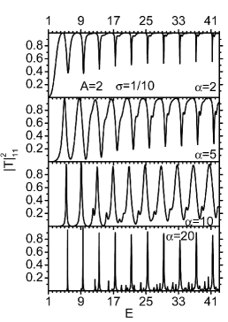
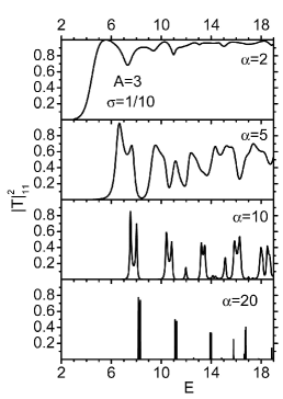
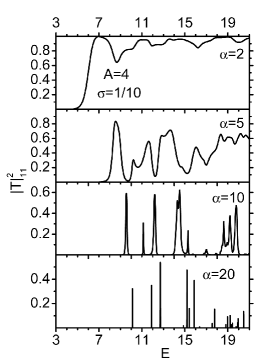
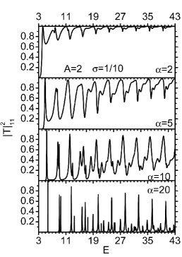
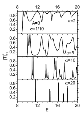
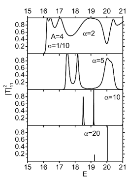
Figure 3: The total transmission probability $|T|^{2}_{11}$ vs energy $E$ (in oscillator units) for the system of $A=2,3,4$ S- (upper panels) and A- (lower panels) particles coupled by the oscillator potential and being initially in the ground cluster state penetrating through the repulsive Gaussian-type potential barriers (24) with $\sigma=0.1$ and $\alpha=2,5,10,20$

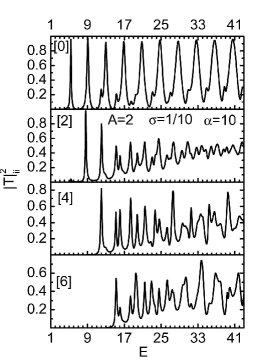
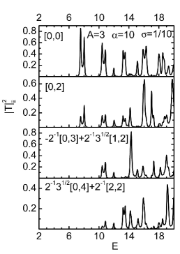
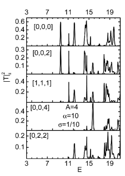
Figure 4: The total transmission probability $|T|^{2}_{ii}$ vs the energy $E$ (in oscillator units) for the system of $A=2,3,4$ particles, coupled by the oscillator potential and being initially in the ground and excited S-states, penetrating through the repulsive Gaussian-type potential barriers (24) with $\sigma=0.1$ and $\alpha=10$. We use the notation of the S-states, $[i_{1},...,i_{A-1}]=1/\sqrt{N_{\beta}}\sum_{i_{1}^{\prime},...,i_{A-1}^{\prime}}\prod\bar{\Phi}_{i_{k}^{\prime}}(\xi_{k})$, with summation over all ($N_{\beta}$) multiset permutations of $i_{1},...,i_{A-1}$ of $A-1$-dimensional oscillator functions [18]

Table 1: Resonance values of the energy $E_{S}$ ($E_{A}$) for S (A) states for $A=2,3,4$ ($\sigma=1/10$, $\alpha=20$) with approximate eigenvalues $E_{i}^{D}$, for the first ten states $i=1,...,10$, calculated using the truncated oscillator basis (D) till $j_{\max}=136,816,1820$ at $A=2,3,4$. The asterisk labels two overlapping peaks of transmission probability

$i$	1	2	3	4	5	6	7	8	9	10
$A=2$
$E_{S}$	5.72	9.06	9.48	12.46	12.57	13.46	15.74	15.78	16.65	17.41
$E_{A}$	5.71	9.06	9.48	12.45	12.57	13.45	15.76∗	15.76∗	16.66	17.40
$E^{D}_{i}$	5.76	9.12	9.53	12.52	12.64	13.52	15.81	15.84	16.73	17.47
$A=3$
$E_{S}$	8.18	11.11		12.60	13.93		14.84	15.79		16.67
	8.31	11.23			14.00		14.88			16.73
$E_{A}$			11.55			14.46			16.18
			11.61			14.56			16.25
$E_{i}^{D}$	8.19	11.09	11.52	12.51	13.86	14.42	14.74	15.67	16.11	16.53
$A=4$
$E_{S}$	10.12	11.89	12.71	14.86	15.19	15.41	15.86	16.37	17.54	17.76
$E^{D31}_{i}$	10.03		12.60	14.71	15.04			16.18	17.34	17.56
$E^{D22}_{i}$		11.76				15.21	15.64

5 Resonance Transmission of a Few Coupled Particles

In the (O) case, i.e., $V^{pair}(x_{ij})=V^{hosc}(x_{ij})$, the solution of the scattering problem described above yields the reflection and transmission amplitudes $R_{ji_{o}}(E)$ and $T_{ji_{o}}(E)$ that enter the asymptotic boundary conditions (9) as unknowns. $|R_{ji_{o}}(E)|^{2}$ ($|T_{ji_{o}}(E)|^{2}$) is the probability of a transition to the state described by the reflected (transmitted) wave and, hence, will be referred as the reflection (transmission) coefficient. Note that $|R_{ji_{o}}(E)|^{2}+|T_{ji_{o}}(E)|^{2}=1$.

In Figs. 3 and 4, we show the energy dependence of the total transmission probability $|T|^{2}_{ii}=\sum_{j=1}^{N_{o}}|T_{ji}(E)|^{2}$. This is the probability of a transition from a chosen state $i$ into any of $N_{o}$ states found from Eq. (21) by solving the boundary-value problem in the Galerkin form, (22) and (25), using the KANTBP 3.0 program [21, 22] on the finite-element grid $\Omega_{\xi}\{-\xi_{0}^{\max},\xi_{0}^{\max}\}$ with $N_{\rm elem}$ fourth-order Lagrange elements between the nodes. For S-solutions at $A=2,3,4$ the following parameters were used: $j_{\max}=13,21,39$, $\xi_{0}^{\max}=9.3,10.5,12.8$, $N_{\rm elem}=664,800,976$, while for A-solutions we used $j_{\max}=13,16,15$, $\xi_{0}^{\max}=9.3,10.5,12.2$, $N_{\rm elem}=664,800,976$ that yield an accuracy of the solutions of an order of the fourth significant figures.

Figure 3 demonstrates non-monotonic behavior of the total transmission probability versus the energy, and the observed resonances are manifestations of the quantum transparency effect. With the barrier height increasing, the peaks become narrower, and their positions shift to higher energies. The multiplet structure of the peaks in the symmetric case is similar to that in the antisymmetric case. For three particles, the major peaks are double, while for two and four particles, they are single. For $A=2$ and $\alpha=10,20$, one can observe the additional multiplets of small peaks.

Figure 4 illustrates the energy dependence of the total transmission probabilities from the exited states. As the energy of the initial excited state increases, the transmission peaks demonstrate a shift towards higher energies, the set of peak positions keeping approximately the same as for the transitions from the ground state and the peaks just replacing each other, like it was observed in the model calculations [12]. For example, for $A=3$, the position of the third peak for transitions from the first two states ($E=10.4167$ and $E=10.4156$) coincides with the position of the first peak for the transitions from the second two states ($E=10.4197$ and $E=10.4298$).

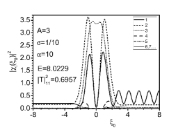
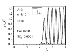
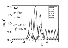
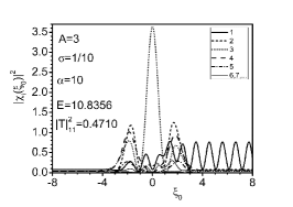
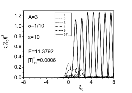
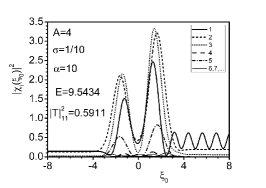
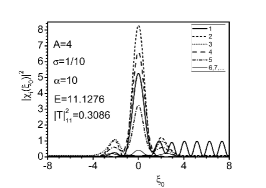
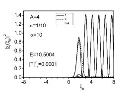
Figure 5: The probability densities $|\chi_{i}(\xi_{0})|^{2}$ for the coefficient functions of the decomposition (21), representing the incident wave function of the ground S-state of the particles at the values of the collision energy $E$ corresponding to individual maxima and minima of the transmission coefficient in Fig. 3. The parameters of the Gaussian barrier are $\alpha=10$ and $\sigma=0.1$

Calculation of energy position of the barrier quasistationary states
In the considered case, the potential barrier $V(x_{i})$ is narrow, and $V^{pair}(x_{ij})=V^{hosc}(x_{ij})$, so that we solve Eq. (1) in the Cartesian coordinates $x_{1},...,x_{A}$ in one of the $2^{A}-2$ subdomains, defined as $p_{i}x_{i}>0$, $p_{i}=\pm 1$, under the Dirichlet conditions (DC): $\Psi(x_{1},...,x_{A})|_{\cup_{i=1}^{A}\{x_{i}=0\}}=0$ at the internal boundaries $\cup_{i=1}^{A}\{x_{i}=0\}$. Here the value $p_{i}=\pm 1$ indicates the location of the $i^{th}$ particle at the right or left side of the barrier, respectively. Thus, in the DC procedure we seek for the solution in the form of a Galerkin expansion over the orthogonal truncated oscillator basis, $\Psi^{D}_{i}({\bf x})\!=\sum_{j=1}^{j_{max}}\bar{\Phi}_{j}({\bf x})\Psi^{D}_{ji}$ composed of $A$-dimensional harmonic oscillator functions $\bar{\Phi}_{j}({\bf x})$, odd in each of the Cartesian coordinates $x_{1},...,x_{A}$ in accordance with the above DCs, with unknown coefficients $\Psi^{D}_{ji}$. As a result, we arrive at the algebraic eigenvalue problem $D\Psi^{\rm D}=\Psi^{\rm D}{E}^{\rm D}$ with a dense real-symmetric $j_{max}\times j_{max}$ matrix. So, in the DC procedure we seek for an approximate solution in one of the potential wells, i.e., we neglect the tunnelling through the barriers between wells. Therefore, we cannot observe the splitting inherent in exact eigenvalues corresponding to S and A eigenstates, differing in permutation symmetry. However, we can explain the mechanism of their appearance and give their classification, which is important, too. This algorithm DC was implemented in CAS MAPLE and FORTRAN environment.
Remark. The DC procedure is similar to solving Eq. (3) in the symmetrized coordinates $\xi_{0},\mbox{\boldmath$\xi$}$ related to the Cartesian ones by Eq. (2), implemented the following two steps:
(i) we approximate the narrow barriers by impenetrable walls $x_{k}(\xi_{0},\mbox{\boldmath$\xi$})=0$;
(ii) we superpose these mutually perpendicular walls with the coordinate hyperplanes using rotations.
Actually, the two approaches yield the same boundary-value problem formulated in different coordinates (1), (3).

The algorithm DC:
                                                                                                                                  
Input:
$A$ is the number of identical particles;
$x_{k}$, $k=1,...,A$ are the Cartesian coordinates of the identical particles;
$p_{k}=\pm 1$ indicates the location of the $k^{th}$ particle ;
$j_{max}$ is the number of the eigenfunctions of A-dimensional harmonic oscillator;
                                                                                                                                  
Output:
$D=\{D_{j^{\prime}j}\}$ is the $j_{max}\times j_{max}$ matrix ;
$E_{i}^{D}$ and $\Psi^{D}_{ji}$ are the real-value eigenenergies and eigenvectors;
                                                                                                                                  
Local:
$\Phi_{j}=\sqrt{2^{A}}\prod_{k=1}^{A}\bar{\Phi}_{i_{k}}(x_{k})$;
$I(i_{k}^{\prime},i_{k})=\int_{0}^{\infty}\bar{\Phi}_{i_{k}^{\prime}}(x)\bar{\Phi}_{i_{k}}(x)dx=\frac{2^{(i_{k}^{\prime}+i_{k})/2}{}_{2}F_{1}(i_{k}^{\prime},i_{k};(2-i_{k}^{\prime}-i_{k})/2;1/2)}{\Gamma((2-i_{k}^{\prime}-i_{k})/2)\sqrt{i_{k}^{\prime}!i_{k}!}};$
$\Gamma(*)$ is the gamma-function, ${}_{2}F_{1}(*,*;*;*)$ is the hypergeometric function;
                                                                                                                                  
1: $Eq:=(-\Delta+\sum(p_{k}x_{k}-p_{k^{\prime}}x_{k^{\prime}})/2A)$;
2: $Eq:=\sqrt{A/(A-1)}(Eq,\Delta\to\Delta/(A/(A-1)),x_{k}\to x_{k}\sqrt[4]{A/(A-1)}$;
3: $Eq:=Eq,p_{k}^{2}\to 1,\Delta=\sum_{k}(x_{k}^{2}-(2n_{k}+1))$;
4: $Eq:=Eq\prod\bar{\Phi}_{i_{k}}(x_{k})$;
5: $Eq:=x_{k}=(\sqrt{i_{k}+1}\bar{\Phi}_{i_{k}+1}(x_{k})+\sqrt{i_{k}}\bar{\Phi}_{i_{k}-1}(x_{k}))/(\sqrt{2}\bar{\Phi}_{i_{k}}(x_{k}))$;
6: for $j,j^{\prime}=1,...,j_{max}$ do
666 $D_{j^{\prime}j}:=\Phi_{i_{k}}(x_{k})\to I(i_{k}^{\prime},i_{k})$;
6: end for
7: $D\Psi^{D}_{ji}=\Psi^{D}_{ji}E_{i}^{D}$ $\to$ $E_{i}^{D}$ and $\Psi^{D}_{ji}$;
                                                                                                                                  

In Table 1, we present the resonance values of the energy $E_{S}$ ($E_{A}$) calculated by solving the boundary-value problem (22) and (25), using the KANTBP 3.0 program, for S (A) states at $A=2,3,4$ $\sigma=1/10$, $\alpha=20$ that correspond to the maxima of transmission coefficients $|T|^{2}_{ii}$ in Fig. 3 up to values of energy $E<18$ and corresponding resonance values of the energy $E_{D}$ calculated by means of the algorithm DC. One can see that the accepted approximation of the narrow barrier with impermeable walls using in the algorithm DC provides the appropriate approximations $E_{i}^{D}$ of the above high accuracy results $E_{S}$ ($E_{A}$) with the error smaller than 2%. Below we give a comparison and qualitative analysis of the obtained results.

For two particles, $A=2$ (see Fig. 1), there are two symmetric potential wells. In each of them both symmetric and asymmetric wave functions are constructed. Since the potential barrier separating the wells is sufficiently high, the appropriate energies are closely spaced, so that each level describes the states of both S and A type. The lower energy levels form a sequence “singlet-doublet-triplet, etc.”, which is seen in Fig. 3. The resonance transmission energies for a pair of particles in S states are lower than that for a pair of those in A states. This is due to the fact that in the vicinity of the collision point, the wave function is zero.

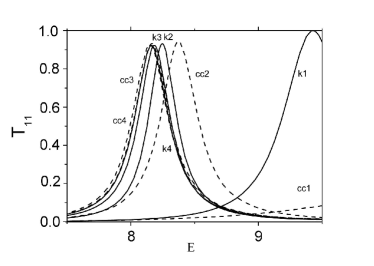
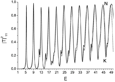
Figure 6: a. The comparison of convergence rate of Galerkin (cc*) and Kantorovich (k*) close-coupling expansions in calculations of transmission coefficient $|T|_{11}^{2}$ for the S-states, $A=2$ at $\alpha=10$, $\sigma=0.1$, like epure of the first peak from Fig. 3. b. The comparison of Galerkin and Kantorovich methods (G=K) with Finite-Difference Numerov method (N)

When $A=3$ there are six similar wells, three of them at each side of the plane $\xi_{0}=0$. The symmetry with respect to the plane $\xi_{0}=0$ explains the presence of doublets. The presence of states with definite symmetry is associated with the fact that the axis $\xi_{0}$ is a third-order symmetry axis. However, in contrast to the case $A=2$, one can obtain either S or A combinations of states. For example, the first four solutions of the problem, in one of the wells (e.g., the one restricted with the pair-collision planes “13” and “23”) possess the dominant components $2\sqrt{2}\bar{\Phi}_{1}(x_{1})\bar{\Phi}_{1}(x_{2})\bar{\Phi}_{1}(x_{3})$, $2(\bar{\Phi}_{1}(x_{1})\bar{\Phi}_{3}(x_{2})+\bar{\Phi}_{3}(x_{1})\bar{\Phi}_{1}(x_{2}))\bar{\Phi}_{1}(x_{3})$, $2(\bar{\Phi}_{1}(x_{1})\bar{\Phi}_{3}(x_{2})-\bar{\Phi}_{3}(x_{1})\bar{\Phi}_{1}(x_{2}))\bar{\Phi}_{1}(x_{3})$, $2\sqrt{2}\bar{\Phi}_{1}(x_{1})\bar{\Phi}_{1}(x_{2})\bar{\Phi}_{3}(x_{3})$. Note that the first, second, and fourth of these functions are symmetric with respect to the permutation $x_{1}\leftrightarrow x_{2}$, while the third one is antisymmetric. Hence, in all six wells using the first four solutions one can obtain six S and two A states.

When $A=4$ there are 14 wells. Six wells at the center correspond to the case when two particles are located at one side of the barrier and the rest two at the other side. The corresponding eigenenergy is denoted $E^{D22}_{i}$. The rest eight wells correspond to the case when one particle is located at one side of the barrier and the rest three at the other side. The corresponding eigenenergy is denoted $E^{D31}_{i}$. For these states, doublets must be observed, similar to the case of three particles. However, the separation between the energy levels is much smaller, because the 4-well groups are strongly separated by two barriers, instead of only one barrier in the case $A=3$.

The necessary condition for the quasi-stationary state being symmetric (antisymmetric) is that the wave functions must be symmetric (antisymmetric) with respect to those coordinates $x_{i}$ and $x_{j}$, for which $p_{i}=p_{j}$.

The effect of quantum transparency is caused by the existence of barrier quasistationary states imbedded in the continuum. Fig. 5 shows that in the case of resonance transmission, the wave functions depending on the center-of-mass variable $\xi_{0}$ are localized in the vicinity of the potential barrier center ($\xi_{0}=0$).

For the energy values corresponding to some of the transmission coefficient peaks in Fig. 3 at $\alpha=10$ within the effective range of barrier potential action, the wave functions demonstrate considerable increase (from two to ten times) of the probability density in comparison with the incident unit flux. This is a fingerprint of quasistationary states, which is not a quantitative definition, but a clear evidence in favor of their presence in the system[23]. In the case of total reflection, the wave functions are localized at the barrier side, on which the wave is incident, and decrease to zero within the effective range of the barrier action.

Note that the explicit explanation of the quantum transparency effect is achieved in the framework of Kantorovich close-coupling equations because of the multi-barrier potential structure of the effective potential, appearing explicitly even in the diagonal or adiabatic approximation, in particular, in the S case for $A=2$ [1, 16]. Nevertheless, in Galerkin close-coupling equations, the multi-barrier potential structure of the effective potential is observed explicitly in the A case (see Fig. 2).

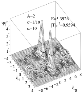
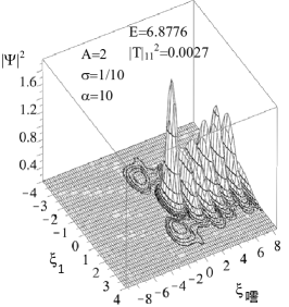
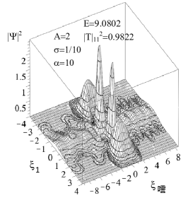
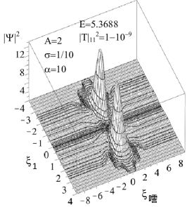
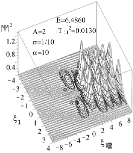
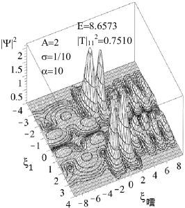
Figure 7: The profiles of probability densities $|\Psi(\xi_{0},\xi_{1})|^{2}$ for the S- (upper panel) and A- (lower panel) states of $A=2$ particles, revealing resonance transmission and total reflection at resonance energies, shown in Figs. 3

As an example, Fig. 6a, which is an epure of Fig. 3, shows the comparison of convergence rates of Galerkin (21) and Kantorovich close-coupling expansions in calculations of transmission coefficient $|T|_{11}^{2}$ for S wave functions, $A=2$ at $\alpha=10$, $\sigma=0.1$. One can see that the diagonal approximation of the Kantorovich method provides better approximations of the positions of the transmission coefficient $|T|_{11}^{2}$ resonance peaks. With the increasing number of basis functions, i.e., the number $j_{\max}$ of close-coupling equations with respect to the center-of-mass coordinates in Galerkin (22) and Kantorovich form, respectively, the convergence rates are similar and confirm the results obtained by solving the problem by means of the Finite-Difference Numerov method in 2D domain [1], see Fig. 6 b. This is true for the considered short-range potentials (24), while for long-range potentials of the Coulomb type, the Kantorovich method can be more efficient [16].

Figure 7 shows the profiles of $|\mbox{\boldmath$\Psi$}|^{2}\equiv|\mbox{\boldmath$\Psi$}_{Em\to}^{(-)}|^{2}$ for the S and A total wave functions of the continuous spectrum in the $(\xi_{0},\xi_{1})$ plane with $A=2$, $\alpha=10$, $\sigma=1/10$ at the resonance energies of the first and the second maximum and the first minimum of the transmission coefficient demonstrating resonance transmission and total reflection, respectively. It is seen that in the case of resonance transmission, the redistribution of energy from the center-mass degree of freedom to the internal (transverse) ones takes place, i.e., the transverse oscillator undergoes a transition from the ground state to the excited state, while in the total reflection, the redistribution of energy is extremely small, and the transverse oscillator returns to infinity in the same state.

6 Conclusion

We considered a model cluster of $A$ identical particles bound by the oscillator-type potential that undergo quantum tunnelling through the short-range repulsive barrier potentials. The model was formulated in the new representation, which we referred as the Symmetrized Coordinate Representation (SCR, see forthcoming paper [18]), that implies construction of symmetric (asymmetric) combinations of oscillator wave functions in new coordinates. The approach was implemented as a complex of the symbolic-numeric algorithms and programs.

For clarity, a system of several identical particles was considered in one-dimensional Euclidian space ($d=1$). We calculated only the spatial part of the wave function, symmetric or antisymmetric under permutation of $A$ identical particles. If necessary, the spin part of the wave function can be introduced using the conventional procedure for more rigorous calculation.

We analyzed the effect of quantum transparency, i.e., the resonance tunnelling of several bound particles through repulsive potential barriers. We demonstrated that this effect is due to the existence of sub-barrier quasistationary states imbedded in the continuum. For the considered type of symmetric Gaussian barrier potential, the energies of the S and A quasistationary states are slightly different because of the similarity of the multiplet structure of oscillator energy levels at a fixed number of particles. This fact explains a similar behavior of transmission coefficients for S and A states shifted by threshold energies. The multiplet structure of these states is varied with increasing the number of particles, e.g., for three particles, the major peaks are double, while for two and four particles, they are single. Our calculations have also shown that with increasing the energy of the initial excited state of few-body clusters, the transmission peaks demonstrate a shift towards higher energies, the set of peak positions keeping approximately the same as for the transitions from the ground state and the peaks just skipping from one position to another.

The proposed approach can be adapted and applied to tetrahedral-symmetric nuclei, quantum diffusion of molecules and micro-clusters through surfaces, and fragmentation mechanism in producing very neutron-rich light nuclei. In connection with the intense search for superheavy nuclei, a particularly significant application of the proposed approach is the mathematically correct analysis of mechanisms of sub-barrier fusion of heavy nuclei and the study of fusion rate enhancement by means of resonance tunnelling.

The authors thank Professors V.P. Gerdt, A. Góźdź, and F.M. Penkov for collaboration. The work was supported by grants 13-602-02 JINR, 11-01-00523 and 13-01-00668 RFBR, 0602/GF MES RK and the Bogoliubov-Infeld program.

References

- [1] Pen’kov, F.M.: Quantum transmittance of barriers for composite particles. JETP 91, 698–705 (2000)
- [2] Pijper, E., Fasolino, A.: Quantum surface diffusion of vibrationally excited molecular dimers. J. Chem. Phys. 126, 014708–1–10 (2007)
- [3] Bondar, D.I., Liu, W.-Ki, Ivanov, M.Yu.: Enhancement and suppression of tunneling by controlling symmetries of a potential barrier. Phys. Rev. A 82, 052112–1–9 (2010)
- [4] Shegelski M.R.A., Pittman, J., Vogt, R., Schaan, B.: Time-dependent trapping of a molecule. European Phys. J. Plus 127, 17–1–13 (2012)
- [5] Ershov, S.N., Danilin, B.V.: Breakup of two-neutron halo nuclei. Phys. Part. Nucl. 39, 1622–1720 (2008)
- [6] Nesterov, A.V., Arickx, F., Broeckhove, J., Vasilevsky, V.S.: Three-cluster description of properties of light nuclei with neutron and proton access within the algebraic version of the resonating group method. Phys. Part. Nucl. 41, 1337–1426 (2010)
- [7] Hofmann, H.: Quantummechanical treatment of the penetration through a two-dimensional fission barrier. Nucl. Phys. A 224, 116–139 (1974)
- [8] Krappe, H.J., Möhring, K.,Nemes, M.C., Rossner, H.: On the interpretation of heavy-ion sub-barrier fusion data. Z. Phys. A 314, 23–31 (1983)
- [9] Cwiok, S., Dudek, J., Nazarewicz, W., Skalski, J., Werner, T.: Single-particle energies, wave functions, quadrupole moments and g-factors in an axially deformed Woods-Saxon potential with applications to the two-centre-type nuclear problems. Comput. Phys. Communications 46, 379–399 (1987)
- [10] Hagino, K., Rowley, N., Kruppa, A.T. A program for coupled-channel calculations with all order couplings for heavy-ion fusion reactions. Comput. Phys. Commun. 123, 143–152 (1999)
- [11] Zagrebaev, V.I., Samarin, V.V.: Near-barrier fusion of heavy nuclei: coupling of channels. Phys. Atom. Nucl. 67, 1462–1477 (2004)
- [12] Ahsan, N., Volya, A.: Quantum tunneling and scattering of a composite object reexamined. Phys. Rev. C 82, 064607–1–19 (2010)
- [13] Shotter, A.C., Shotter, M.D.: Quantum mechanical tunneling of composite particle systems: Linkage to sub-barrier nuclear reactions. Phys. Rev. C 83, 054621–1–11 (2011)
- [14] Shilov, V.M.: Sub-barrier fusion of intermediate and heavy nuclear systems. arXiv:1012.3683 [nucl-th] Phys. Atom. Nucl. 75, 485–490 (2012)
- [15] Chuluunbaatar, O., Gusev, A.A., Derbov, V.L., Krassovitskiy, P.M., Vinitsky, S.I.: Channeling problem for charged particles produced by confining environment. Phys. Atom. Nucl. 72, 768–778 (2009)
- [16] Gusev, A.A., Vinitsky, S.I., Chuluunbaatar, O., Gerdt, V.P., Rostovtsev, V.A.: Symbolic-numerical algorithms to solve the quantum tunneling problem for a coupled pair of ions. LNCS 6885, 175–191 (2011)
- [17] Gusev, A.A., Chuluunbaatar, O., Vinitsky, S.I.: Computational scheme for calculating reflection and transmission matrices, and corresponding wave functions of multichannel scattering problems. In: Uvarova, L.A. (ed.) Proc. Second International Conference “The Modeling of Non-linear Processes and Systems”, (Yanus, Moscow, 2011), ISBN 978-5-8037-0541-3.
- [18] Gusev, A., Vinitsky, S., Chuluunbaatar, O., Rostovtsev, V., Hai, L., Derbov, V., Góźdź, A., Klimov, E.: Symbolic-numerical algorithm for generating cluster eigenfunctions: identical particles with pair oscillator interactions, presented in this issue
- [19] Vinitsky, S.I., Gerdt, V.P., Gusev, A.A., Kaschiev, M.S., Rostovtsev, V.A., Samoilov, V.N., Tupikova, T.V., Chuluunbaatar, O.: A symbolic-numerical algorithm for the computation of matrix elements in the parametric eigenvalue problem, Programming and Computer Software 33, 105–116 (2007)
- [20] Bunge, C.F.: Fast eigensolver for dense real-symmetric matrices. Comput. Phys. Communications 138, 92–100, (2001)
- [21] Chuluunbaatar, O., Gusev, A.A., Vinitsky, S.I., Abrashkevich, A.G.: KANTBP 2.0: New version of a program for computing energy levels, reaction matrix and radial wave functions in the coupled-channel hyperspherical adiabatic approach, Comput. Phys. Commun. 179, 685–693 (2008)
- [22] Chuluunbaatar, O., Gusev, A.A., Vinitsky, S.I., Abrashkevich, A.G.: KANTBP 3.0 - New version of a program for computing energy levels, reflection and transmission matrices, and corresponding wave functions in the coupled-channel adiabatic approach, Program library “JINRLIB”, http://wwwinfo.jinr.ru/programs/jinrlib/kantbp/indexe.html
- [23] de Carvalho, C.A.A., Nussenzweig, H.M.: Time delay. Phys. Rept. 364, 83–174 (2002)