Galaxy redshift surveys with sparse sampling

Abstract

Survey observations of the three-dimensional locations of galaxies are a powerful approach to measure the distribution of matter in the universe, which can be used to learn about the nature of dark energy, physics of inflation, neutrino masses, etc. A competitive survey, however, requires a large volume (e.g., $V_{\rm survey}\sim 10~{}{\rm Gpc}^{3}$) to be covered, and thus tends to be expensive. A “sparse sampling” method offers a more affordable solution to this problem: within a survey footprint covering a given survey volume, $V_{\rm survey}$, we observe only a fraction of the volume. The distribution of observed regions should be chosen such that their separation is smaller than the length scale corresponding to the wavenumber of interest. Then one can recover the power spectrum of galaxies with precision expected for a survey covering a volume of $V_{\rm survey}$ (rather than the volume of the sum of observed regions) with the number density of galaxies given by the total number of observed galaxies divided by $V_{\rm survey}$ (rather than the number density of galaxies within an observed region). We find that regularly-spaced sampling yields an unbiased power spectrum with no window function effect, and deviations from regularly-spaced sampling, which are unavoidable in realistic surveys, introduce calculable window function effects and increase the uncertainties of the recovered power spectrum. On the other hand, we show that the two-point correlation function (pair counting) is not affected by sparse sampling. While we discuss the sparse sampling method within the context of the forthcoming Hobby-Eberly Telescope Dark Energy Experiment, the method is general and can be applied to other galaxy surveys.

1 Introduction

How do we measure the large-scale distribution of matter in the universe? Broadly speaking, there are two classes of methods: (1) to measure locations of collapsed objects (galaxies and clusters of galaxies), and (2) to measure the distribution of the intervening matter by gravitational lensing or absorption lines (e.g., Lyman-$\alpha$ forest). In this paper, we focus on the first class (although our one-dimensional study may have some relevance to the Lyman-$\alpha$ forest), and ask the question, “What is the most efficient way to measure three-dimensional locations of collapsed objects?”

Ideally, one aims to measure angular positions and redshifts of all galaxies down to a certain limiting line flux or magnitude over the full sky; however, this approach is usually too expensive to carry out in practice. The most time-consuming aspect is the spectroscopic observations required to determine redshifts. A conventional method has been to execute less-expensive imaging surveys over some fraction of the full sky, and use certain criteria to select candidates for spectroscopic observations. Still, in some cases too many candidates remain for feasible spectroscopic observations. Also, for multi-object spectrographs, collisions of fibers/slits make it difficult to observe crowded (over-dense) regions. To observe all galaxies in these regions, one must visit the same area more than once, requiring a further selection process. As one wishes to avoid introducing artificial clustering of galaxies due to selection effects, selection of candidates is done such that the outcome is a fair sample of the underlying distribution of galaxies, i.e., Poisson sampling of galaxies selected from the imaging survey data [1]. This method works and has been repeatedly used in the past: recent examples include the Sloan Digital Sky Survey (SDSS; [2, 3]), the Two-degree Field Galaxy Redshift Survey (2dFGRS; [4]), the WiggleZ Dark Energy Survey [5], and the VIMOS Public Extragalactic Redshift Survey (VIPERS; [6]).

There is a way to avoid pre-selection of targets. With the advent of Integral Field Unit (IFU) spectrographs, it is now possible to obtain blind, multiple spectra of all points in the sky simultaneously in the two-dimensional field-of-view of the instrument without target pre-selection. For example, the Visible Integral-Field Replicable Unit Spectrograph (VIRUS; [7, 8]), which will outfit the 10-m Hobby-Eberly Telescope (HET; [9]) at McDonald Observatory in West Texas, consists of 75 IFUs. Each IFU has 448 fibers and feeds one unit with two spectrographs. 150 spectrographs (33,600 fibers) are being built and will be used for a forthcoming galaxy survey called the Hobby-Eberly Telescope Dark Energy Experiment (HETDEX; [10]). HETDEX is a blind spectroscopic survey of emission-line galaxies in a high-redshift universe. Specifically, HETDEX will observe spectra between 3500 and 5500 Å at the resolution of $R\sim 700$ in order to detect approximately 0.8 million Lyman-$\alpha$ emitting galaxies over the redshift range of $z=1.9-3.5$. The total volume covered by the survey footprints is approximately 9 Gpc³.

While it is in principle possible to obtain spectra (hence redshifts) of all galaxies in the sky down to a certain limiting line flux and within a certain redshift range by simply “tiling the sky with IFUs,” in practice it still requires a great commitment of resources.

At this point, we first must decide what we would want to accomplish with our galaxy survey data. In this paper, we shall focus on measuring the power spectrum of galaxies, $P_{g}(k)$, from three-dimensional locations of galaxies found by a galaxy redshift survey such as HETDEX. If the focus is to measure the power spectrum of galaxies, the observational requirements are somewhat relaxed. The fractional statistical r.m.s. uncertainty of the measured power spectrum is given by $\delta P_{g}(k)/P_{g}(k)\propto V_{\rm survey}^{-1/2}(1+[n_{g}P_{g}(k)]^{-1})$, where $n_{g}$ is the number density of observed galaxies and $V_{\rm survey}$ is a survey volume. The first and second terms within the parenthesis represent uncertainties from sample variance and shot noise, respectively. We would not be able to reduce the uncertainty of the measured power spectrum significantly by observing more galaxies once we have the number density of galaxies that satisfies $n_{g}P_{g}(k)>1$. At that point, the only way to reduce the uncertainty is to cover more volume.

The exact definition of $V_{\rm survey}$ requires some thoughts. Suppose that we divide a large volume, $V_{\rm survey}$, into smaller regions each having a volume of $V_{\rm small}$, which are separated by distances comparable to the size of each volume. (When the smaller non-overlapping regions are embedded in the larger volume, $V_{\rm survey}$, the sum of $V_{\rm small}$ is smaller than $V_{\rm survey}$.) Is the survey volume $V_{\rm survey}$, or the sum of $V_{\rm small}$? The answer depends on the wavenumbers at which we measure $P_{g}(k)$. If we are interested in measuring the power spectrum on length scales much smaller than the size of smaller volumes, $k\gg 2\pi V_{\rm small}^{-1/3}$, then the survey volume would be the sum of $V_{\rm small}$. On the other hand, to reconstruct a plane-wave fluctuation having a given wavenumber, one would not need to have a full sample of the plane wave. The Nyquist sampling theorem states that one can completely reconstruct a plane-wave fluctuation as long as it is sampled at the rate twice the wavenumber of the plane wave. Therefore, if we choose the distribution of smaller regions properly, we can reconstruct long-wavelength fluctuations by sparsely sampling $V_{\rm survey}$ without loss of information; thus, the survey volume in this case is equal to $V_{\rm survey}$ despite the fact that the observations cover only a fraction of $V_{\rm survey}$.

A number of questions arise. For example, what is the optimal distribution of smaller regions? Should we distribute them regularly, or randomly? In this paper, we shall address questions related to this “sparse sampling method” as applied to galaxy redshift surveys. Specifically, we shall discuss the sparse sampling method within the context of HETDEX [10]; however, our discussion is sufficiently general so that it can be applied to other galaxy surveys measuring the power spectrum. Similar issues have been studied in [11, 12].

This paper is organized as follows. In section 2, we construct a relation between the observed galaxy power spectrum and the underlying one, making clear how the selection function of the sparse sampling enters into the relation. In section 3, we analyze a toy one-dimensional example to understand the basic properties of the power spectrum measured from sparsely-sampled density fields. In section 4, we investigate a toy two-dimensional example to explore the effects of shapes and orientations of observed regions. In section 5, we use log-normal realizations of semi-realistic density fields in three dimensions to investigate the remaining effects of sparse sampling in detail. We also study how sparse sampling of a realistic galaxy survey may affect the observed Baryon Acoustic Oscillations (BAOs) and the constraints on cosmological parameters. In section 6, we study the effect of sparse sampling on the two-point correlation function. We conclude in section 7. In appendix A, we derive the one-dimensional window function effect for Gaussian perturbations to the regularly-sparse sampling. In appendix B, we describe our log-normal simulations of density fields. In appendix C, we present our Gaussian realizations for the power spectrum with window functions.

2 Power spectrum and window function

Galaxy redshift surveys measure three-dimensional locations of galaxies, from which one can determine two-point correlation functions. The two-point correlation function in real space can be estimated from the observed locations directly, while computation of the two-point correlation function in Fourier space (power spectrum) using a Fast Fourier Transform requires an estimate of local number density of galaxies at regular grid points. Using an appropriate density assignment scheme (such as the nearest-grid-point (NGP) density assignment; the cloud-in-cell (CIC) density assignment; etc. See [13]), one can measure local density fields of observed galaxies, $n_{g}({\bf r})$.

The observed number density is a product of the true, underlying number density of galaxies of a given population for a given limiting magnitude or line flux, $n({\bf r})$, and the so-called “selection function,” $W({\bf r})$:

$$n_{g}({\bf r})=n({\bf r})W({\bf r}).$$ (2.1)

The observed density fluctuation is defined as (see eq. 2.1.3 of [14])

$$\delta_{g}({\bf r})\equiv\frac{n_{g}({\bf r})-\bar{n}_{g}({\bf r})}{\left[\int d^{3}r~{}\bar{n}^{2}_{g}({\bf r})\right]^{1/2}}.$$ (2.2)

Here, $\bar{n}_{g}({\bf r})\equiv\bar{n}(z)W({\bf r})$ is an estimate of the local mean number density of galaxies, and $\bar{n}(z)$ is the global mean of $n({\bf r})$ at a given redshift calculated from, e.g., a controlled field where $W({\bf r})$ is normalized to be unity.

In this paper, we shall focus only on the spherically-averaged (monopole) power spectrum. Fourier transforming $\delta_{g}$, we calculate the observed power spectrum, $\hat{P}_{g}(k)$, by

$$\hat{P}_{g}(k)\equiv\frac{1}{N_{k}}\sum_{i=1}^{N_{k}}\left|\delta_{g}({\bf k}_{i})\right|^{2},$$ (2.3)

where $N_{k}$ is the number of Fourier meshes for which $|{\bf k}_{i}|$ lies within a given wavenumber bin, i.e., $k-\delta k/2\leq|{\bf k}_{i}|<k+\delta k/2$. The expectation value of $\hat{P}_{g}(k)$ is then given by (see eq. 2.1.6 of [14])

$$\langle\hat{P}_{g}(k)\rangle=\frac{1}{W_{\rm sq}}\int\frac{d^{3}q}{(2\pi)^{3}}~{}P({\bf q})|W({\bf k}-{\bf q})|^{2}+P_{\rm shot},$$ (2.4)

where $P({\bf q})$ is the true, underlying power spectrum of galaxies of a given population for a given limiting magnitude or line flux, $W_{\rm sq}$ is the normalization factor given by $W_{\rm sq}\equiv\int d^{3}r~{}\bar{n}^{2}(z)W^{2}({\bf r})$, and $P_{\rm shot}$ is the shot noise:

$$P_{\rm shot}\equiv\frac{\int d^{3}r~{}\bar{n}(z)W^{2}({\bf r})}{\int d^{3}r~{}\bar{n}^{2}(z)W^{2}({\bf r})}.$$ (2.5)

Here in the derivation, we have ignored the effects of density assignments. However, in our numerical results, we do take the density assignments into account following the procedures in ref. [13].

In the sparse-sampling approach, there are gaps (i.e., $W({\bf r})=0$) between observed fields. Therefore, our goal is to determine how the sparse sampling affects the observed power spectrum and its uncertainties. For simplicity, throughout this paper, we shall assume that $\bar{n}(z)$ is independent of $z$, i.e. $\bar{n}(z)=\bar{n}$. Thus $W_{\rm sq}=\bar{n}^{2}\int d^{3}r~{}W^{2}({\bf r})=(2\pi)^{-3}\bar{n}^{2}\int d^{3}k~{}|W({\bf k})|^{2}$.

3 One-dimensional study

3.1 Regularly-spaced sparse sampling

First, let us examine a toy example of a one-dimensional density field. Suppose that we observe $N$ one-dimensional non-overlapping regions, each having a size of $d$. The selection function is given by the sum of $N$ top-hat functions: $W(x)=\sum_{m=1}^{N}\theta(d/2-|x-x_{c,m}|)$, where $\theta(y)=1$ for $y\geq 0$ and 0 otherwise, and $x_{c,m}$ is the position of the center of the $m^{\rm th}$ region. Fourier-transforming the selection function, one finds $W(k)=d\sum_{m=1}^{N}{\rm sinc}(kd/2)e^{-ikx_{c,m}}$. (${\rm sinc}(x)=\sin(x)/x$.) For regularly-spaced regions with a separation between the centers given by $r$, one finds

$$W(k)=\frac{dL}{r}\frac{{\rm sinc}(kd/2){\rm sinc}(kL/2)}{{\rm sinc}(kr/2)},$$ (3.1)

where $L=Nr$ is the survey length. The one-dimensional window function is shown in figure 1 for survey parameters of $L=1000~{}h^{-1}~{}{\rm Mpc}$, $d=1~{}h^{-1}~{}{\rm Mpc}$, and $r=2~{}h^{-1}~{}{\rm Mpc}$.

For wavelengths much greater than the size of the smaller regions, $kd\ll 1$, and the separation between the region centers, $kr\ll 1$, the window function becomes $W(k)\propto{\rm sinc}(kL/2)$, which is what one would expect for a contiguous survey ($r=d$).

Figure 1: (Left panel) One-dimensional window function of a regularly-spaced sparse sampling, $W(k)$ (see eq. 3.1), for $0\leq k\leq 0.2~{}h~{}{\rm Mpc}^{-1}$. (Right panel) Same as the left panel, but for $3.0\leq k\leq 3.2~{}h~{}{\rm Mpc}^{-1}$. The survey parameters are $L=1000~{}h^{-1}~{}{\rm Mpc}$, $d=1~{}h^{-1}~{}{\rm Mpc}$, and $r=2~{}h^{-1}~{}{\rm Mpc}$.

The key behavior of this window function is that it diverges at $kr=2m\pi$ where $m$ is an arbitrary non-zero integer. This property may bias the observed power spectrum, and the effect can be quantified by the one-dimensional version of eq. 2.4, i.e.,

$$\langle\hat{P}_{g}(k)\rangle=\frac{1}{W_{\rm sq}}\int\frac{dq}{2\pi}~{}P(|q|)|W(k-q)|^{2},$$ (3.2)

as $\langle\hat{P}_{g}(k)\rangle$ receives contributions from $P(k)$ as well as from $P(|k\pm 2m\pi/r|)$. (We have ignored the shot noise here for simplicity.)

However, there is an easy solution to this problem. When we compute density fields from locations of galaxies, we assign density values to meshes (which we call “density meshes”). If we choose the size of density meshes, $H=L/N_{\rm mesh}$, such that the Nyquist frequency, $k_{Nyq}=\pi/H$, is smaller than $2\pi/r$, then the above integral receives contributions from the main peak ($k-q=0$) but does not receive contributions from the other peaks ($k-q=\pm 2\pi/r$) of the window function, and thus $\langle\hat{P}_{g}(k)\rangle-P_{\rm shot}$ becomes unbiased, i.e., regularly-spaced sparse sampling returns an unbiased power spectrum when the size of the density mesh is so large/coarse ($H>r/2$) that it does not resolve separations between observed regions. Mathematically, eq. 3.2 is modified as

$$\langle\hat{P}_{g}(k)\rangle=\frac{1}{W_{\rm sq,mesh}}\int\frac{dq}{2\pi}~{}P(|q|)|W(k-q)|^{2}|W_{\rm mesh}(k-q)|^{2},$$ (3.3)

where $W_{\rm mesh}(k)$ is the Fourier transform of the density assignment scheme and $W_{\rm sq,mesh}=\int\frac{dk}{2\pi}~{}|W(k)|^{2}|W_{\rm mesh}(k)|^{2}$. For CIC, $W_{\rm mesh}(k)={\rm sinc}^{2}(kH/2)$. Therefore, all peaks in the window function with wavenumber greater than $2\pi/H$ are suppressed. To compute this expression, we use Fourier transform: we first create a one-dimensional Fourier-space window function, $W(k)$, with $d=1~{}h^{-1}~{}{\rm Mpc}$, $r=2~{}h^{-1}~{}{\rm Mpc}$, and $L=1000~{}h^{-1}~{}{\rm Mpc}$ (i.e., $N=500$). We then compute $|W(k)|^{2}|W_{\rm mesh}(k)|^{2}$, Fourier transform it to real space, multiply the result by the Fourier transform of the underlying power spectrum, and finally Fourier transform the product back to obtain $\langle\hat{P}_{g}(k)\rangle$.

Figure 2: (Top panel) The thick dashed and dotted lines show the expectation values of the observed power spectrum, $\langle\hat{P}_{g}(k)\rangle$, computed from 500 and 1200 density meshes, respectively (the total survey length, $L$, is divided into 500 and 1200 meshes). The survey parameters are $L=1000~{}h^{-1}~{}{\rm Mpc}$, $r=2~{}h^{-1}~{}{\rm Mpc}$, and $d=1~{}h^{-1}~{}{\rm Mpc}$. The solid line shows the underlying power spectrum, $P(k)$. (Bottom panel) Ratios of $\langle\hat{P}_{g}(k)\rangle$ to $P(k)$.

In figure 2, we display two power spectra computed from eq. 3.2 with two density meshes. For 500 and 1200 meshes, the linear sizes of each mesh are $H=2.000$ and $0.833~{}h^{-1}~{}{\rm Mpc}$, respectively. (Note that the survey length, $L$, is the same for both mesh sizes.) As $r/2=1~{}h^{-1}~{}{\rm Mpc}$, the former does not resolve separations between observed regions, while the latter does. As a result, we find that the former yields an unbiased power spectrum, while the latter is significantly biased.

This bias in the power spectrum we find here can be understood by recalling that $\langle\hat{P}_{g}(k)\rangle$ receives contributions from $P(k)$ as well as from $P(|k\pm 2m\pi/r|)$ with $2\pi/r\simeq 3.1~{}h~{}{\rm Mpc}^{-1}$. As $P(k)$ is a decreasing function of $k$ for $k\gtrsim 10^{-2}~{}h~{}{\rm Mpc}^{-1}$, contributions from $P(|k\pm 2m\pi/r|)$ are much smaller than those from $P(k)$ for $k\ll 2\pi/r$. Therefore, eq. 3.2 is approximately given by

$$\langle\hat{P}_{g}(k)\rangle\approx\frac{1}{W_{\rm sq}}\frac{k_{F}}{2\pi}~{}P(k)|W(0)|^{2},$$ (3.4)

for $k\ll 2\pi/r$. Here, $k_{F}=2\pi/L$ is the fundamental frequency. For 1200 meshes, we have $W_{\rm sq}=330.533$ and $W(0)=dL/r=500$, which gives $\langle\hat{P}_{g}(k)\rangle\simeq 0.824P(k)$, in agreement with the numerical result shown in figure 2.

As we move to smaller scales, a contribution of $P(|k-2\pi/r|)$ becomes important. For example, $P(|k-2\pi/r|)$ becomes equal to $P(k)$ for $k=\pi/r\simeq 1.5~{}h~{}{\rm Mpc}^{-1}$, in agreement with the result in figure 2. At $k>1.5~{}h~{}{\rm Mpc}^{-1}$, the contribution of $P(|k-2\pi/r|)$ exceeds that of $P(k)$, enhancing $\langle P_{g}(k)\rangle$ above $P(k)$.

3.2 Perturbations to regularly-spaced sparse sampling

Due to various observational constraints, it is often not possible to have perfectly regular separations between observed regions. To study the effect of deviations from regular spacing, we perturb the center of the $a^{\rm th}$ observed region by $\epsilon_{a}$, where $\epsilon_{a}$ is a Gaussian variable with zero mean, $\langle\epsilon_{a}\rangle=0$, and the correlation function given by $\langle\epsilon_{a}\epsilon_{b}\rangle=\sigma_{\epsilon}^{2}\delta_{ab}$. The expectation value of the window function squared is given by

$$\langle\left|W(k)\right|^{2}\rangle = \left[d\ {\rm sinc}\left(\frac{kd}{2}\right)\right]^{2}\sum_{a=1}^{N}\sum_{b=1}^{N}e^{-ik\bar{x}_{a}}e^{ik\bar{x}_{b}}\langle e^{-ik\epsilon_{a}}e^{ik\epsilon_{b}}\rangle$$ (3.5)

$$= \left[d\ {\rm sinc}\left(\frac{kd}{2}\right)\right]^{2}\left[N+e^{-k^{2}\sigma_{\epsilon}^{2}}\sum_{a\neq b}e^{-ik(\bar{x}_{a}-\bar{x}_{b})}\right],$$

where $\bar{x}_{a}$ denotes the unperturbed, regularly-spaced position of the $a^{\rm th}$ region. The derivation of this result is given in appendix A.

As the perturbations of the center of the observed regions would suppress the observed power spectrum on large scales, we quantify the effect of non-regularity by computing the large-scale suppression of the power spectrum as a function of the standard deviation of perturbations, $\sigma_{\epsilon}$. We compute $W_{\rm sq}$ by the discrete sum as $W_{\rm sq}=\frac{k_{F}}{2\pi}\sum_{n=-n_{Nyq}}^{n_{Nyq}}\langle|W(nk_{F})|^{2}\rangle|W_{\rm mesh}(nk_{F})|^{2}$, where $n_{Nyq}$ is equal to the Nyquist frequency divided by the fundamental frequency, $k_{F}=2\pi/L$.

Figure 3: Ratio of the expectation value of the observed power spectrum, $\langle\hat{P}_{g}(k)\rangle$, to the underlying power spectrum, $P(k)$, computed from eq. 3.9 for $k\ll 2\pi/r$ as a function of the magnitude of perturbations to the positions of the centers of observed regions, $\sigma_{\epsilon}$. The survey parameters are $L=1000~{}h^{-1}~{}{\rm Mpc}$, $r=2~{}h^{-1}~{}{\rm Mpc}$, and $d=1~{}h^{-1}~{}{\rm Mpc}$, and 500 density meshes are used. The solid line is computed from eq. 3.9. while the dashed line is an approximate fitting formula, $\exp\left[-(\sigma_{\epsilon}/\alpha r)^{2}\right]$, where $\alpha=0.8$.

For $k=0$ ($n=0$), the last term of eq. 3.5 becomes

$$\sum_{a\neq b}e^{-ik(\bar{x}_{a}-\bar{x}_{b})}=\sum_{a\neq b}1=2\sum_{a=1}^{N-1}\sum_{b=0}^{a-1}1=N^{2}-N.$$ (3.6)

For $k\neq 0$ ($n\neq 0$),

$$\sum_{a\neq b}e^{-ik(\bar{x}_{a}-\bar{x}_{b})} = \sum_{a\neq b}e^{-ikr(a-b)}=2\sum_{a=1}^{N-1}\sum_{b=0}^{a-1}\cos\left[kr(a-b)\right]$$ (3.7)

$$= \frac{-1+N-N\cos(kr)+\cos(Nkr)}{-1+\cos(kr)},$$

where we have defined $\bar{x}_{a}=x_{0}+ar$ ($0\leq a\leq N-1$) and $x_{0}=(-L+r)/2$. Recalling $L=Nr$, one finds $\cos(Nkr)=\cos(nk_{F}L)=\cos(2n\pi)=1$; thus, the right hand side of eq. 3.7 is equal to $-N$. Using these results,

$$W_{\rm sq}=\frac{k_{F}}{2\pi}\Bigg{\{}d^{2}N^{2}+2d^{2}N\sum_{n=1}^{n_{Nyq}}{\rm sinc}^{2}\left(\frac{nk_{F}d}{2}\right)\left[1-e^{-(nk_{F}\sigma_{\epsilon})^{2}}\right]|W_{\rm mesh}(nk_{F})|^{2}\Bigg{\}}.$$ (3.8)

Inserting eq. 3.8 into eq. 3.4,

$$\frac{\langle\hat{P}_{g}(k)\rangle}{P(k)}=\frac{N}{N+2\sum_{n=1}^{n_{Nyq}}{\rm sinc}^{2}(nk_{F}d/2)\left[1-e^{-(nk_{F}\sigma_{\epsilon})^{2}}\right]|W_{\rm mesh}(nk_{F})|^{2}},$$ (3.9)

for $k\ll 2\pi/r$. Figure 3 shows $\langle\hat{P}_{g}(k)\rangle/P(k)$ as a function of $\sigma_{\epsilon}$. The solid line is computed from eq. 3.9, while the dashed line is an approximate fitting formula, $\exp\left[-(\sigma_{\epsilon}/\alpha r)^{2}\right]$, where $\alpha=0.8$.

We find that, if perturbations are much smaller than the separation between observed regions (i.e., $\sigma_{\epsilon}\ll r$), they have a negligible impact on the power spectrum. As $\sigma_{\epsilon}$ becomes larger, the observed large-scale power is suppressed with respect to the underlying one. This exercise shows that the optimal strategy for sparse sampling is to make the distribution of observed regions as regularly separated as possible.

4 Two-dimensional study

4.1 Tiling the sky with shots

We now extend the toy model to two dimensions. Suppose that we have the focal plane of a telescope which we wish to fill with many IFUs. Each IFU consists of densely packed optical fibers. (For HETDEX, each IFU consists of 448 fibers.) While it would be ideal to fill the focal plane entirely with IFUs without any gaps, limited resources and technical practicality usually prevent doing so. (For HETDEX, 75 IFUs are placed on the focal plane filling only a quarter of the focal plane area.) Therefore, motivated by the study in the previous section, we place our IFUs such that the focal plane contains IFUs which are separated by regular spacings.

Let us now define the term “shot,” as the projection of the focal plane onto the sky. We conduct a galaxy survey by tiling the sky with many shots. The question we wish to answer in this section is, “how should we tile the sky with shots?”

The left panel of figure 4 shows one example. Each small square represents one IFU. Objects will only be detected if they fall within one IFU. The IFUs are approximately arranged in a hexagonal pattern. There are (at least) two reasons to prefer a hexagon over a square or a circle. First, due to the HET specifics, the image quality and throughput tend to degrade toward the edges of the focal plane. Therefore, a circle or a hexagon is preferred over a square, as the length of diagonal of a square is longer than that of the side of a square. Second, we wish to perform a galaxy survey by tiling the sky. As one cannot completely tile the sky by circles without significant overlaps, a square or a hexagon is preferred over a circle. These constraints identify a hexagon as the best choice.

Figure 4: (Left panel) Distribution of IFUs (shown by squares) for a single “shot,” which is the focal plane projected onto the sky. There are 64 IFUs in this example. Each IFU covers the comoving size of $1~{}h^{-1}~{}{\rm Mpc}$, and they are regularly separated by $2~{}h^{-1}~{}{\rm Mpc}$. (Middle panel) Survey area tiled without any gaps between shots (each shot consists of 64 IFUs as shown in the left panel). The dotted line shows the survey boundary, whose area is $64~{}h^{-1}~{}{\rm Mpc}\times 64~{}h^{-1}~{}{\rm Mpc}$. The survey area shown here is 10 times smaller than what is actually used by the calculations presented in the main text. Separations between the shot centers are $16~{}h^{-1}~{}{\rm Mpc}$ along $x$ and $y$ directions. (Right panel) Survey area tiled with gaps and random rotations. Separations between the shot centers are $17.6~{}h^{-1}~{}{\rm Mpc}$. Orientations of shots are rotated randomly by angles between $-10^{\circ}$ and $+10^{\circ}$. The survey area is $70.4~{}h^{-1}~{}{\rm Mpc}\times 70.4~{}h^{-1}~{}{\rm Mpc}$.

In the plane-parallel approximation, we set the center-to-center separation between IFUs to be $2~{}h^{-1}~{}{\rm Mpc}$, and the size of each IFU to be $d=1~{}h^{-1}~{}{\rm Mpc}$. ($1~{}h^{-1}~{}{\rm Mpc}$ corresponds to roughly 0.88 arcminute at $z=2.2$.) With this configuration, the filling fraction (ratio of the area of IFUs to the area of a shot) is roughly 25%, so approximately $1/4$ of galaxies within a single shot will be observed.

For a single IFU, the real-space selection function is a two-dimensional top-hat function. In Fourier space, the window function of a single IFU becomes

$$W_{\rm IFU}({\bf k})=d^{2}{\rm sinc}\left(\frac{k_{x}d}{2}\right){\rm sinc}\left(\frac{k_{y}d}{2}\right)\ .$$ (4.1)

The window function of a single shot (see the left panel of figure 4) is then given by $W_{\rm shot}({\bf k})=\sum_{m=1}^{64}W_{\rm IFU}({\bf k})e^{-i{\bf k}\cdot{\bf r}_{m}}$, where ${\bf r}_{m}$ is the position of the $m^{\rm th}$ IFU with respect to the center of the shot.

We tile the survey area by many shots. Suppose that we use $N$ shots to fill a given survey area, and the $n^{\rm th}$ shot is located at ${\bf L}_{n}$ with respect to the origin of the survey area. Ignoring the possibility that each shot can be rotated (we shall return to this possibility shortly), the final two-dimensional window function is

$$W({\bf k})=\sum_{n=1}^{N}W_{\rm shot}({\bf k})e^{-i{\bf k}\cdot{\bf L}_{n}}=W_{\rm IFU}({\bf k})\sum_{n=1}^{N}\sum_{m=1}^{64}e^{-i{\bf k}\cdot({\bf L}_{n}+{\bf r}_{m})}\ ,$$ (4.2)

where ${\bf L}_{n}+{\bf r}_{m}$ is the position of the $m^{\rm th}$ IFU in the $n^{\rm th}$ shot. Once the window function is computed, one can calculate the observed power spectrum by the two-dimensional version of eq. 3.3, i.e.,

$$\langle\hat{P}_{g}(k)\rangle=\frac{1}{W_{\rm sq}}\int\frac{d^{2}q}{(2\pi)^{2}}~{}P(|{\bf q}|)|W({\bf k}-{\bf q})|^{2}|W_{\rm mesh}({\bf k}-{\bf q})|^{2}\ ,$$ (4.3)

where $W_{\rm mesh}({\bf k})={\rm sinc}^{2}(k_{x}H/2){\rm sinc}^{2}(k_{y}H/2)$ for CIC. We use this equation to study how the observed power spectrum is biased for a given distribution of shots in the sky.

First, let us consider the case in which shots completely cover the survey area without gaps between shots (but there are still small separations between IFUs), as shown in the middle panel of figure 4. For this example, the separation between shots is $16~{}h^{-1}~{}{\rm Mpc}$ along the $x$ and $y$ directions. We tile the survey area by 41 shots in the odd rows and 40 shots in the even rows, giving $41\times 21+40\times 20=1661$ shots in total. The survey area is 640 ($=16\times 40$) $h^{-1}$ Mpc by 640 $h^{-1}$ Mpc. For the further analysis we only consider a square-shaped subregion (shown by the dotted lines in the middle panel of figure 4) of the actually covered region. This avoids the complications of the unevenly covered regions around the survey edges and simplifies the window function. We count the IFUs if their centers are within the subregion. If IFUs are partially covered at the edge of the subregion, the window functions of the IFUs would vary, but this effect is negligible.

To compute the window function, we apply eq. 4.2. We then convolve the underlying power spectrum with the window function using the Fourier transformation: we multiply the Fourier transform of $|W({\mathbf{k}})|^{2}$ by the Fourier transform of the underlying power spectrum, and compute the inverse Fourier transform of the product. We set the size of the density mesh to be $2~{}h^{-1}~{}{\rm Mpc}$, which is large enough so that the separation between IFUs within a shot does not bias the observed power spectrum according to our one-dimensional study given in the previous section.

Since there are no gaps between shots, the survey area is sampled regularly by IFUs which are separated by $2~{}h^{-1}~{}{\rm Mpc}$. Therefore, as expected from our one-dimensional study, the observed power spectrum is unbiased, which is shown as the dotted line in figure 5. However, while the observed power spectrum is unbiased by sparse sampling, the uncertainties of the power spectrum increase, as the number of observed galaxies is less than what would be obtained from a contiguous survey. We shall investigate the effect of sparse sampling on the uncertainties of the power spectrum in section 5.

Figure 5: Ratios of the observed power spectrum, $\langle\hat{P}_{g}(k)\rangle$, to the underlying power spectrum, $P(k)$. The dotted, solid, and dashed lines show $\langle\hat{P}_{g}(k)\rangle/P(k)$ with tiled shots without gaps, shots with gaps but no rotation, and random rotations between $-10^{\circ}$ and $+10^{\circ}$ (i.e., the right panel of figure 4), respectively.

Now let us consider the case in which there are small gaps between shots. As an example, we increase the separation between shots to $|\delta{\mathbf{r}}|=17.6~{}h^{-1}~{}{\rm Mpc}$ along the $x$ and $y$ directions, which is 10% larger than the previous case in which the shots completely fill the survey area without gaps. Here, $\delta{\mathbf{r}}\equiv{\mathbf{r}}_{i}-{\mathbf{r}}_{j}$. The number of shots (1661) is the same as before, and the survey area increases to 704 ($=17.6\times 40$) $h^{-1}~{}{\rm Mpc}$ by $704~{}h^{-1}~{}{\rm Mpc}$.

The solid line in figure 5 displays the result of this example. We find $\sim 9$% suppression of the power spectrum on large scales, and an enhancement of power on small scales. The reason for the suppression and enhancement are exactly the same as that for the one-dimensional study: gaps between shots introduce an additional regular spacing scale, yielding the suppression and enhancement of the observed power spectrum with respect to the underlying one. Therefore, one should avoid having any gaps between shots in order to minimize the window function effect. One can estimate the magnitude of the large-scale suppression via the two-dimensional version of eq. 3.4, i.e.,

$$\langle\hat{P}_{g}(k)\rangle\approx\frac{1}{W_{\rm sq}}\left(\frac{k_{F}}{2\pi}\right)^{2}~{}P(k)|W(0)|^{2}\ .$$ (4.4)

Here, $W(0)=d^{2}N_{\rm IFU}$ and $N_{\rm IFU}$ is the total number of regions covered by IFUs in the survey area. Using $N_{\rm IFU}=102720$, $W_{\rm sq}=23388$, and $(k_{F}/2\pi)=1/(704~{}h^{-1}$ Mpc), the above formula produces a large-scale suppression of 0.910, which is in an excellent agreement with the result shown in figure 5, which was obtained directly from eq. 4.3.

4.2 Randomly rotated shots

Let us now consider the case in which there are small gaps between shots, and the orientations of shots are randomly rotated, as shown in the right panel of figure 4. For a single rotated shot, the window function is $W_{\rm shot,rot}({\bf k})=W_{\rm shot}(R[\theta]{\bf k})$, where $R[{\theta}]$ is a rotation matrix and $\theta$ is a rotation angle with respect to the positive $x$ direction. For $N$ shots with different rotations, we can extend eq. 4.2 as

$$W({\bf k}) = \sum_{n=1}^{N}W_{\rm shot,rot}({\bf k})e^{-i{\bf k}\cdot{\bf L}_{n}}=\sum_{n=1}^{N}W_{\rm shot}(R[\theta_{n}]{\bf k})e^{-i{\bf k}\cdot{\bf L}_{n}}$$ (4.5)

$$= \sum_{n=1}^{N}W_{\rm IFU}(R[\theta_{n}]{\bf k})e^{-i{\bf k}\cdot{\bf L}_{n}}\sum_{m=1}^{64}e^{-i(R[\theta_{n}]{\bf k})\cdot{\bf r}_{m}}\ ,$$

where $\theta_{n}$ is the rotation angle of the $n^{\rm th}$ shot.

The dashed line in figure 5 shows the result of the rotated shots. Here, we have rotated shots randomly by angles between $-10^{\circ}$ and $+10^{\circ}$. We find that the rotation affects the power spectrum only slightly ($\lesssim 1$%) and thus is sub-dominant compared to the effect of gaps between shots. Rotations sometimes move IFUs out of the bounded area, causing a small change in the window function. The extra suppression on large scales for the random rotation is due to the fewer IFUs in the survey area. This large-scale suppression can be estimated by eq. 4.4 as well.

Our two-dimensional study demonstrates that gaps between shots have much larger impact on the observed power spectrum than small rotations. As gaps between shots are typically larger than the size of the density mesh, the optimal strategy for sparse sampling is to avoid having gaps between shots.

4.3 Shot with a hole in the middle

Figure 6: (Left panel) A distribution of IFUs within a shot with a hole in the middle of the pattern. There are 58 IFUs. (Right panel) Ratio of the observed power spectrum, $\langle\hat{P}_{g}(k)\rangle$, to the underlying power spectrum, $P(k)$, for the distribution of IFUs shown on the left panel. There are no gaps between shots, and thus the window function effect is solely due to the hole in the middle.

Finally, let us consider a specific case for HETDEX. There will be an instrument with higher dispersion in the center of the HET focal plane, and the layout of IFUs would contain a hole with size of 6 IFUs in the middle of the pattern.

The left panel of figure 6 shows the distribution of IFUs on the focal plane with no coverage in the middle of the field, and the right panel shows the effect of the hole on the observed power spectrum. There are no gaps between shots, but the existence of the hole creates an additional artificial scale in the window function. For the case explored here, in which the area of a hole is about 10% of the focal plane area, we find $\sim 7\%$ suppression of the power spectrum on large scales, and an enhancement of power on small scales. The impact of the hole in the middle of a shot is as large as that of 10% gaps between shots.

Again, one can estimate the magnitude of the large-scale suppression by eq. 4.4. Using $N_{\rm IFU}=93040$, $W_{\rm sq}=22640.1$, and $k_{F}/(2\pi)=1/640~{}h^{-1}~{}{\rm Mpc}$, we find the large-scale suppression of $0.933$, which is in good agreement with the result shown in figure 6.

5 Three-dimensional study

5.1 Effect of curvature of the sky

We now study a semi-realistic, three-dimensional model. Suppose that we undertake a galaxy survey whose survey footprint is bounded by right ascension (RA), declination (DEC), and redshift. Throughout this paper, we shall use the term “footprint” to denote the outermost boundary of the survey, which contains many sub-volumes of observed regions.

As the celestial sphere is spherical, the survey volume is no longer a cube in Cartesian coordinates. This means that one should, ideally, use the spherical Fourier-Bessel decomposition (rather than the usual Fourier transform) to treat density fields in radial and tangential directions separately [15, 16, 17].

However, in this paper we shall continue to use the fast Fourier transform approach. The spherical Fourier-Bessel decomposition is still new in the large-scale structure community, and much work is left to do before we fully understand the optimal implementation of the method. On the other hand, the Fourier transform is easier to implement, computationally less expensive, and is also the conventional way to compute the power spectrum. (The Fourier transform has been used by all of the major galaxy surveys such as 2dFGRS, SDSS, WiggleZ, and VIPERS.)

We use a cuboidal box which is just large enough to contain the entire survey footprint. This choice produces a non-trivial selection function $W({\bf r})$: namely, $W({\bf r})=1$ if ${\bf r}$ lies within the survey footprint, and 0 otherwise.

To study the effect of the curvature of the celestial sphere, we generate 1000 sets of mock catalogues of galaxies for a HETDEX-like survey. The survey footprint covers $34.1^{\circ}\times 7.5^{\circ}$ on the sky and a redshift range of $1.9\leq z\leq 2.5$. The central coordinates of the survey footprint in the sky are $(\mbox{RA},\mbox{DEC})=(13^{\rm h},53^{\circ})$ (J2000).

The input galaxy power spectrum for simulations is a non-linear power spectrum at $z=2.2$ based on the third-order perturbation theory with non-linear bias [18, 19]. The bias parameters are $b_{1}=2.2$, $b_{2}=0.671$, and $P_{0}=72.13~{}h^{-3}~{}{\rm Mpc}^{3}$, and the number density of galaxies is $\bar{n}=2.95\times 10^{-3}~{}h^{3}~{}{\rm Mpc^{-3}}$. We use log-normal realizations of the input power spectrum to generate mock catalogues, and describe our method to generate log-normal realizations in appendix B.

Once galaxies are created in the cuboidal simulation box in Cartesian coordinates, we select all galaxies lying within the survey footprint. The side lengths of the simulation box along $x$, $y$, and $z$ directions are $L_{x}=2481.94~{}h^{-1}~{}{\rm Mpc}$, $L_{y}=540.122~{}h^{-1}~{}{\rm Mpc}$, and $L_{z}=759.653~{}h^{-1}~{}{\rm Mpc}$, respectively. (For the reasons given in footnote 6, this is approximately a third of the volume to be surveyed by HETDEX.) Figure 7 shows the distribution of galaxies within the survey footprint of one realization. The survey volume is no longer cuboidal in Cartesian coordinates, and the $z$ direction is not parallel to the redshift direction due to curvature of the sky. The galaxies within the survey footprint are approximately 2/3 of all galaxies in the simulation box. From now on, we shall use the term “geometry selection” for galaxies within the survey footprint, and “no selection” for all galaxies within the entire simulation box. The “geometry selection” galaxies are a subset of the “no selection” galaxies.

Figure 7: A log-normal realization of galaxies. (Left panel) A slice on the RA-redshift plane with $52.974^{\circ}\leq\mbox{DEC}\leq 53.026^{\circ}$. (Right panel) A slice on the $x$-$z$ plane of the simulation box in Cartesian coordinates with $-1.350\leq y\leq 1.350~{}h^{-1}~{}{\rm Mpc}$.

To measure the power spectra from log-normal realizations, we use the CIC density assignment to compute the local number density of galaxies per density mesh, and then use eq. 2.2 to compute the density contrast field, $\delta_{g}$. The number of random samples used for computing $\bar{n}_{g}$ in eq. 2.2 is approximately 2500 times that of galaxies, so that the Poisson error in the estimate of $\bar{n}_{g}$ is negligible. Once the real-space density contrast is constructed, it is Fourier transformed, and the power spectrum computed by eq. 2.3. To reduce the sample variance we generate 1000 log-normal realizations, calculate the averages of the power spectra of the “no selection” and “geometry selection” cases, and compute the ratio of the two, $\bar{P}_{\rm geometry}(k)/\bar{P}_{\rm no}(k)$. We denote quantities averaged over 1000 realizations with the over bar.

Figure 8: Ratios of the average of the geometry selection power spectra, $\bar{P}_{\rm geometry}(k)$, to the average of the underlying (“no selection”) power spectra, $\bar{P}_{\rm no}(k)$, computed from 1000 log-normal realizations (solid line; the error bars show the errors on the mean). The dashed line shows the average of the underlying power spectra convolved with the window function squared, which agrees well with the direct measurement. Oscillatory features seen in $0.05\lesssim k\lesssim 0.5~{}h~{}{\rm Mpc}^{-1}$ are not noise but real: they are produced by a smearing of BAO features due to the window function. See section 5.3 for details.

The solid line in figure 9 shows this ratio, $\bar{P}_{\rm geometry}(k)/\bar{P}_{\rm no}(k)$. The ratio is less than unity on large scales ($k\lesssim 0.2~{}h~{}{\rm Mpc}^{-1}$), whereas it approaches approximately unity on small scales. This result is not surprising: the geometry selection has no effect on the window function when the distance between galaxy pairs is smaller than the curvature scale, and thus the geometry selection affects the observed galaxy power spectrum only on large scales. This effect is well known and presented in any galaxy surveys which are analyzed using the usual Fourier transform technique.

It is straightforward to model this effect: convolve the squared Fourier transform of the geometry selection function (see eq. 2.4). To compute the real-space selection function, we create random particles in the simulation box, and select only the particles within the survey footprint. The real-space selection function is then proportional to the number density of the selected particles, i.e., $W_{\rm num}({\bf r})\propto n_{s}({\bf r})$. The function, $W_{\rm num}({\bf r})$, does not need to be normalized, as the normalization factor is canceled by $W_{\rm sq}$ in the denominator of eq. 2.4.

The dashed line in figure 9 shows the average of the “no selection” power spectra measured from 1000 realizations convolved with the squared window functions divided by the average of the “no selection” power spectra. The convolved power spectrum agrees well with the direct measurement from the simulation shown by the solid line.

5.2 Effect of sparse sampling

Figure 9: (Left panel) Distribution of IFUs within a shot. Each square represents an IFU, and there are 80 IFUs. Six central IFUs in the left panel have been removed.

Figure 10: Example shot positions in the sky. Each hexagon represents a shot location. There are 4060 shots within the $34.1^{\circ}\times 7.5^{\circ}$ survey area. As HET is more efficient for constant-declination observations, the shot positions are generated under the constant-declination requirement. There are no gaps or overlaps between shots at ${\rm DEC}=51.25^{\circ}$, whereas there are some gaps and overlaps at lower and higher declinations, respectively.

We now apply the sparse sampling method to our simulations. Figure 9 shows two example distributions of IFUs within a single shot, and figure 10 shows locations of shots in the northern sky. These locations resemble, but are not the same as, the planned HETDEX survey footprint.

The shots are placed on constant declination rows, as HET is more efficient for constant-declination surveys. Due to curvature of the celestial sphere, it is impractical to design a realistic galaxy survey completely tiling the survey area without any gaps or overlaps. In order to minimize excessive irregularities, gaps, or overlaps, we first tile the shots without gaps or overlaps at ${\rm DEC}=51.25^{\circ}$. Then, for the adjacent (up and down) rows, the neighboring hexagon shots are placed in phase to keep the shot locations regular. We keep this procedure until the shots reach the boundary of the survey area. Because of curvature of the celestial sphere, in higher declination rows some shots overlap and in lower declination rows some shots have small gaps. The window function due to these effects will be quantified later.

As we focus on the angular selection effect of sparse sampling in this paper, we shall assume that all the IFUs have equal sensitivity at all wavelengths for detecting galaxies. As this assumption will not hold in reality, there will be a radial window function effect from the line-of-sight selection. We have studied the radial window function of the HETDEX survey using the actual sensitivity of IFUs measured from the HETDEX Pilot Survey [20, 21], and found that the radial selection function yields $|W(k_{z})|^{2}/|W(0)|^{2}\lesssim 10^{-4}$, which is much smaller than that of the angular selection.

Figure 11: Ratios of the averages of the 80-IFU (solid) and 74-IFU (dashed) selected power spectra to the average of the geometry selection power spectra. The solid line shows the window function effect due to gaps between shots toward lower declinations caused by curvature of the sky (see figure 10), while the dashed line shows the additional window function effect caused by a hole in the middle of the focal plane (see the right panel of figure 9). The error bars show the errors on the mean. The oscillatory features seen in this figure are not noise but real: they are caused by a smearing of BAO features due to the window function. See section 5.3 for details.

We select galaxies lying inside the IFUs, measure the power spectra from 1000 log-normal realizations, and average the results. To separate the effect of sparse sampling from that of geometry selection, we divide the averages of the 80-IFU and 74-IFU selected power spectra by the average of the geometry selection power spectra (rather than by the underlying power spectrum). Figure 11 shows the ratios of the averages of the 80-IFU (without a hole; solid line) and 74-IFU (with a hole; dashed line) selected power spectra to the average of the geometry selection power spectra. Ideally, if shot positions are regular without any gaps and there is no large central hole (as in the left panel of figure 9), there is no window function effect, as our one-dimensional and two-dimensional studies have previously shown. However, because of curvature of the celestial sphere, small gaps appear between shots at lower declinations (see figure 10), which yields a slight, $\sim 2\%$ suppression on large scales. On the other hand, for the 74 IFUs shot with a central hole, we observe a larger window function effect, as expected from our two-dimensional study.

The window function effect due to a central hole for the three-dimensional case is smaller than that for the two-dimensional case, which is due to the smaller fraction of the focal plane area occupied by the central hole (6 out of 80 here versus 6 out of 64 before).

5.3 Baryon Acoustic Oscillation

Thus far, we have focused our attention on the effects of sparse sampling and curvature of the sky on the overall shape of the observed galaxy power spectrum, and found a smooth suppression of the power on large scales. In this section, we shall focus on the effects of sparse sampling and curvature of the sky on sharper features in the power spectrum, i.e., BAO features.

To investigate how the window functions may affect BAOs, we extract BAOs from the underlying power spectrum convolved with the window functions from various cases such as the geometry selection and sparse sampling. We extract BAO features as follows. We first fit the power spectra estimated from various cases to a smooth power spectrum without BAO features as

$$P_{\rm smooth}(k)=\sum_{i}c_{i}S_{i}(k)\ ,$$ (5.1)

where $S_{i}$ is the $i^{\rm th}$ cubic spline function, and $c_{i}$ is a coefficient of $S_{i}$. We find $c_{i}$ by minimizing $\chi^{2}=\sum_{j}[\langle\hat{P}_{g}(k_{j})\rangle-\sum_{i}c_{i}S_{i}(k_{j})]^{2}/\sigma^{2}(k_{j})$, where $\sigma^{2}(k_{j})\equiv[\langle\hat{P}_{g}(k_{j})\rangle+P_{\rm shot}]^{2}/N(k_{j})$ and $N(k_{j})$ is the number of independent Fourier modes in the $j^{\rm th}$ bin. We set the fitting range to be $0.005~{}h~{}{\rm Mpc}^{-1}\leq k\leq 0.4~{}h~{}{\rm Mpc}^{-1}$, and there are 12 parameters to be fitted. We then extract BAOs as

$${\rm BAO}(k)\equiv\langle\hat{P}_{g}(k)\rangle-P_{\rm smooth}(k).$$ (5.2)

Figure 12: Smearing of BAO features due to various window function effects. The solid line shows the underlying BAOs divided by the smooth power spectrum with no selection function. The dot-dashed line shows a smearing due to the application of Fourier transform to a spherical sky (“geometry selection”). The long-dashed line shows an additional smearing due to gaps between shots in lower declinations due to curvature of the sky (see figure 10). The short-dashed line, which lies on top of the long-dashed line, demonstrates that a central hole in the focal plane (see the right panel of figure 9) does not introduce a significant additional smearing of BAO features. The BAOs shown here are extracted from the convolution of the underlying power spectrum and the window functions.

In figure 12, we show the BAOs extracted from the underlying power spectrum convolved with various window functions, divided by the smooth power spectrum. We find that the BAO features are smeared: while the phase of the BAO is unaffected, the amplitude has decreased. The biggest smearing arises from the geometry selection (the dot-dashed line; which has nothing to do with sparse sampling but is caused by the application of Fourier transform to spherical sky), which yields 12% reduction in the amplitude of BAO features. Once again, this effect is not new and is present in any survey results obtained from the Fourier transform approach (see e.g. [2, 3, 4, 5]). One should in principle be able to remove this effect by using the spherical Fourier-Bessel transform [15, 16, 17]; we leave it as future work.

A smaller effect is produced by irregularities of the shot positions due to curvature of the celestial sphere, which yield a further 5% reduction in the amplitude of BAOs (the long-dashed line). The central hole does not appear to introduce any additional smearing (the short-dashed line, which lies on top of the long-dashed line) to the BAOs.

Smearing of BAOs occurs when BAOs are convolved with a smooth window function with a broad width. The window function of the geometry selection does exactly this. However, the window function of the sparse sampling is neither smooth nor broad (see figure 1). Therefore, the sparse sampling with completely regular separations causes no smearing of BAOs. We have seen this already from figures 2, 5, and 6, where the ratios of the BAOs and the smooth power spectrum on BAO scales do not have any structures. (I.e., both the BAOs and the smooth power spectrum are suppressed by the same factor.) However, deviations from regularity introduce a small additional smearing, as shown by the dashed line in figure 12.

5.4 Constraint on the BAO peak position

5.4.1 Finding the dilation parameter

In the previous subsection, we have shown that the amplitude of BAOs is smeared by the window function, mainly due to curvature of the sky. Because of the smearing, the statistical power of the BAOs for cosmological parameter estimations will degrade in proportion to the magnitude of smearing; namely, if the amplitude of BAOs is reduced by 10%, the parameter constraint also degrades by 10%, assuming that the uncertainty does not change. (If the signal-to-noise decreases by 10% without changing the noise, it is the signal that decreases by 10%. Then, the uncertainty in the parameters also increases by 10%.) Moreover, because of the window function, the adjacent Fourier modes of the power spectrum may be correlated, and thus the parameter constraint degrades further. In the following, we shall investigate how curvature of the sky and the sparse sampling affect the constraint on the BAO peak position.

In order to study this issue, we estimate the so-called “dilation parameter ,” $\alpha$, of BAOs, i.e., ${\rm BAO}(k)\to{\rm BAO}(k/\alpha)$ [22], from 1000 log-normal simulations. We find $\alpha$ and the parameters characterizing the smooth component, $c_{i}$, from each realization by minimizing

$$\chi^{2}=\sum_{ij}\left[\hat{P}_{g}(k_{i})-P_{\rm smooth}(k_{i})-{\rm BAO}\left(\frac{k_{i}}{\alpha}\right)\right]\left[\hat{P}_{g}(k_{j})-P_{\rm smooth}(k_{j})-{\rm BAO}\left(\frac{k_{j}}{\alpha}\right)\right]C_{ij}^{-1}\ ,$$ (5.3)

where $P_{\rm smooth}(k)$ is given in eq. 5.1, $C_{ij}$ is the covariance matrix computed from the power spectra of 1000 log-normal realizations, and the BAO model here already includes the smearing due to the window function effects, as shown in figure 12.

5.4.2 Structure of the covariance matrix

It is necessary to compute $\chi^{2}$ using the full covariance matrix (instead of only the diagonal elements of $C_{ij}$, i.e., the variance), as the window function correlates adjacent Fourier modes. In figure  13, we show the absolute values of the correlation coefficient, $|C_{ij}|/\sqrt{C_{ii}C_{jj}}$, for Gaussian (see appendix C) and log-normal realizations. The wavenumbers shown here are $0.05\leq k\leq 0.35~{}h~{}{\rm Mpc^{-1}}$, with increments of $0.005~{}h~{}{\rm Mpc}^{-1}$.

The errors of the inverse covariance matrix $C^{-1}_{ij}$ are given by $\langle\Delta(C^{-1})_{ij}^{2}\rangle=A(C^{-1})_{ij}^{2}+B[(C^{-1})_{ii}(C^{-1})_{jj}+(C^{-1})_{ij}^{2}]$ [23]. In the Gaussian limit, $A=2/[(N_{s}-N_{b}-1)(N_{s}-N_{b}-4)]$ and $B=(N_{s}-N_{b}-2)/[(N_{s}-N_{b}-1)(N_{s}-N_{b}-4)]$, where $N_{s}$ and $N_{b}$ are the number of realizations and bins, respectively. In our case, $N_{s}=1000$ and $N_{b}=61$, yielding $A\simeq 2.28\times 10^{-6}$ and $B\simeq 1.07\times 10^{-3}$. Thus, we estimate the errors on the inverse covariance matrix as $\sqrt{\langle\Delta(C^{-1})_{ij}^{2}\rangle}\simeq 0.0327\sqrt{[(C^{-1})_{ii}(C^{-1})_{jj}+(C^{-1})_{ij}^{2}]}$. Since the dominant components of the inverse covariance matrix are the diagonal elements, the errors are bounded by $0.0327\leq\sqrt{\langle\Delta(C^{-1})_{ij}^{2}\rangle/[(C^{-1})_{ii}(C^{-1})_{jj}]}\leq 0.0462$. As the inverse covariance matrix is dominated by the diagonal elements, a few percent errors with respect to the diagonal elements of the off-diagonal elements can be safely neglected. To test the convergence, we also run 5000 log-normal realizations. We find that the results of 5000 log-normal realizations are quite similar to those of 1000 log-normal realizations, and the conclusions of the paper are unchanged.

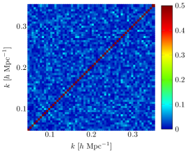
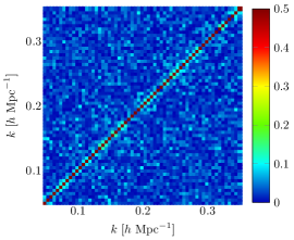
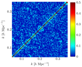
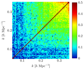
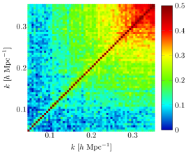
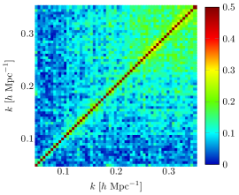
Figure 13: Absolute values of the correlation coefficients of the covariance matrix, $|C_{ij}|/\sqrt{C_{ii}C_{jj}}$. We show the correlation coefficients for no selection (left panels), the geometry selection (middle panels), and the selection of 74 IFUs with a central hole (right panels). While we display the absolute values of the correlation coefficients, they are mostly positive. The diagonal elements are equal to unity, while the colors show values from 0 to 0.5. (Top panels) Correlation coefficients computed from 1000 Gaussian realizations, which do not include the effect of shot noise (see appendix C). These figures clearly show positive correlations of adjacent Fourier modes due to the window function effects. (Bottom panels) Correlation coefficients from 1000 log-normal realizations, which include the effect of shot noise. These figures show additional positive correlations due to the non-Gaussian nature of the underlying density fields. The bottom-right panel shows smaller correlation coefficients for off-diagonal elements, as the diagonal elements are enhanced by the larger shot noise without significantly increasing off-diagonal elements. (Recall that approximately 25% of galaxies in the survey footprint are selected by 74 IFUs with a central hole, which results in much larger shot noise for the 74-IFU-selection.)

First, let us study the correlation coefficients computed from Gaussian realizations. These realizations do not include the effect of shot noise (see appendix C), and thus they show purely the effects of window functions. For no selection (top left panel), the off-diagonal elements of the correlation coefficients are negligible; this is because the connected four-point function of $\delta({\bf k})$, which produces non-zero off-diagonal elements of the covariance matrix, vanishes for Gaussian random fields. (By definition the connected four-point function is the four-point function minus the Gaussian contribution.) However, this is true only when we do not have window functions. In the presence of window functions, the mode functions (i.e., $e^{i\mathbf{k}\cdot\mathbf{x}}$) are no longer orthogonal, and thus adjacent Fourier modes become positively correlated. We find this positive correlation for the geometry selection (top middle panel), as well as for the sparse sampling of 74 IFUs with a hole (top right panel). The correlations of adjacent Fourier modes are typically 10%, and are similar for both the geometry selection and the geometry plus IFU selection. These results demonstrate that the primary source for the correlations is the geometry selection, rather than the sparse sampling.

Next, let us study the correlation coefficients computed from log-normal realizations (see appendix B), which include the effect of shot noise. For no selection (bottom left panel), there are significant positive correlations between Fourier modes due to the non-Gaussian nature of the underlying density fields. For the geometry selection (bottom middle panel), we find additional positive correlations for the adjacent Fourier modes (which is the same as those we found from Gaussian realizations), as well as for a broad range of wavenumbers on small scales.

For the sparse sampling of 74 IFUs with a hole (bottom right panel), the off-diagonal correlation coefficients become smaller than those of the geometry selection. This result is due to the larger shot noise: there are much fewer galaxies selected by sparse sampling, and thus the diagonal elements of the covariance matrix increase relative to the off-diagonal elements. (The shot noise contributes only to the diagonal elements of the covariance matrix.) As the correlation coefficients are normalized to unity in the diagonal elements, the off-diagonal elements become correspondingly smaller. The actual (non-normalized) values of the off-diagonal elements of the covariance matrix are slightly larger than those of the no-selection and geometry- selection cases, in agreement with the results of Gaussian realizations.

5.4.3 Uncertainty on $\alpha$: Fisher matrix versus direct fitting

Figure 14: Same as figure 12, but for the average of BAOs extracted from 1000 realizations of our log-normal simulations. The error bars show the errors on the mean for 74 IFUs with a hole. The error bars for no- and geometry-selections are smaller.

With the covariance matrix computed, we now minimize $\chi^{2}$ given in eq. 5.3 to find the values for $\alpha$ from 1000 realizations, and compute the 1-$\sigma$ uncertainty in $\alpha$. We set the fitting range to be $0.05~{}h~{}{\rm Mpc}^{-1}\leq k\leq 0.35~{}h~{}{\rm Mpc}^{-1}$, which contains most of the BAO features. There are 61 data points, and 11 parameters (10 for $c_{i}$ and 1 for $\alpha$) to be fitted in total. We use the Levenberg-Marquardt method ([24]) to find the minimum of $\chi^{2}$.

The averages of BAOs extracted from 1000 realizations of our log-normal simulations for various window functions are shown in figure 14, which are in agreement with the models in figure 12.

Using 1000 log-normal realizations, we find that the average of $\alpha$ from 1000 realizations is unity to within the uncertainty of simulations (i.e., the standard deviation divided by $\sqrt{1000}$), indicating that our method yields an unbiased estimate of $\alpha$. The 1-$\sigma$ uncertainties in $\alpha$ we find are 0.92%, 1.17%, and 1.95% for no selection, geometry selection, and sparse sampling of 74 IFUs with a central hole, respectively.

To check whether log-normal realizations agree with expectations, let us compare these values with the expectations from the simplest treatment of galaxy surveys that is widely used by the cosmology community. Ignoring the off-diagonal elements of the covariance matrix or the effect of window functions on the diagonal elements of the covariance matrix, the uncertainty in $\alpha$ is given by

$$\frac{1}{({\rm Err}[\alpha])^{2}}=V_{\rm survey}\int_{k_{min}}^{k_{max}}\frac{d^{3}k}{2(2\pi)^{3}}\frac{1}{[\bar{P}_{g}(k)+1/\bar{n}_{g}]^{2}}\left[\frac{\partial{\rm BAO}(k)}{\partial{\rm ln}k}\right]^{2}\ .$$ (5.4)

Here, $\bar{P}_{g}(k)$ is the average power spectrum of 1000 log-normal realizations with corresponding window functions, and ${\rm BAO}(k)$ is given by the BAOs extracted from the underlying power spectrum convolved with window functions, as shown in figure 12.

In this formula, we need the survey volume, $V_{\rm survey}$, and the galaxy number density, $\bar{n}_{g}$. The meaning of these quantities is clear for the no-selection and geometry-selection cases: as all galaxies within the cuboid simulation box are observed, the volume of no-selection case is $1.018~{}h^{-3}~{}{\rm Gpc}^{3}$. For the geometry selection, only galaxies lying within the survey footprint are observed, and thus the volume is $0.722~{}h^{-3}~{}{\rm Gpc}^{3}$ (255.75 square degrees in the sky and $1.9<z<2.5$). As the observed regions are contiguous, the number density is identical for both the no-selection and geometry-selection cases. We have $\bar{n}_{g}=2.95\times 10^{-3}~{}h^{3}~{}{\rm Mpc}^{-3}$. (There are 3.003 million and 2.130 million galaxies for no-selection and geometry-selection cases, respectively.)

What about in the sparse sampling case? The results we have presented in this paper so far suggest that, provided that the wavenumber of interest is sufficiently smaller than the wavenumber corresponding to the separation between IFUs ($k\simeq 3.14~{}h~{}{\rm Mpc}^{-1}$), the sparse sampling approach can yield the same results as the survey which has the volume within the survey footprint (i.e., the outermost boundary of the survey), and the number density of galaxies which is the total number of observed galaxies divided by the volume of the footprint. We thus take the survey volume to be the volume of the footprint, $V_{\rm survey}=0.722~{}h^{-3}~{}{\rm Gpc}^{3}$, and the galaxy number density for the selection by 74 IFUs with a hole to be $\bar{n}_{g}=0.667\times 10^{-3}~{}h^{3}~{}{\rm Mpc}^{-3}$. (There are 0.482 million observed galaxies for the selection by 74 IFUs with a central hole.)

Inserting these values into eq. 5.4, we find the expected uncertainties in $\alpha$ of 0.86%, 1.21%, and 1.90% for no selection, geometry selection, and sparse sampling of 74 IFUs with a central hole, respectively. These numbers are in good agreement with 0.92%, 1.17%, and 1.95% we find from the direct fitting of log-normal realizations.

The Fisher matrix given by eq. 5.4 does not include the off-diagonal elements of the covariance matrix or the fact that we simultaneously fit 11 parameters. To include these effects, we generalize eq. 5.4 to [25]

$$F_{ij}=\sum_{m,n}\frac{\partial\langle\hat{P}_{g}(k_{m})\rangle}{\partial\theta_{i}}\frac{\partial\langle\hat{P}_{g}(k_{n})\rangle}{\partial\theta_{j}}C^{-1}_{mn}\ ,$$ (5.5)

where $F_{ij}$ is the Fisher matrix, and $\theta_{i}$ denotes the $i^{\rm th}$ parameter. As there are 11 parameters, the dimension of the Fisher matrix is $11\times 11$, and we set $\theta_{0}\equiv\alpha$ and $\theta_{i}\equiv c_{i}$. The 1-$\sigma$ uncertainty in $\alpha$ is then given by $\sqrt{(F^{-1})_{00}}$. We find ${\rm Err}[\alpha]=$ 0.90%, 1.13%, and 1.76% for no selection, the geometry selection, and the sparse sampling of 74 IFUs with a central hole, respectively.

From these results, we conclude that the uncertainty in $\alpha$ achieved by the sparse sampling is comparable to that of a galaxy survey with the survey volume of the footprint, and the number density given by the total number of observed galaxies within the footprint divided by the volume of the footprint.

5.4.4 Significance of BAO detection with sparse sampling

In section 5.4.3, we presented the averages of the extracted BAOs from 1000 log-normal realizations. In this subsection, we shall show the extracted BAOs from six log-normal realizations as examples, and discuss the significance of BAO detection with sparse sampling.

Figure 15: Extracted BAOs from six randomly-chosen log-normal realizations with sparse sampling. The “$\sigma$” labels in the upper right of each panel show “significance of BAOs detection,” calculated as $\sqrt{\chi^{2}_{\rm null}-\chi^{2}}$, where $\chi^{2}$ and $\chi^{2}_{\rm null}$ are the minimum $\chi^{2}$ values with and without BAOs included in the model. In the bottom-right panel, we find $\chi^{2}>\chi^{2}_{\rm null}$ (i.e., we do not detect BAOs) and thus we show $-\sqrt{\chi^{2}-\chi^{2}_{\rm null}}$.

In figure 15, we display the extracted BAOs, $\hat{P}_{g}(k)-P_{\rm smooth}(k)$, from six randomly-chosen log-normal realizations with sparse sampling. The error bars are given by the square root of diagonal elements of the covariance matrix directly measured from our log-normal realizations. The values of $\sigma$ is the significance of BAO detection.

We quantify the significance of BAO detection for each realization by $S/N=\sqrt{\chi^{2}_{\rm null}-\chi^{2}}$, where $\chi^{2}$ is the minimum $\chi^{2}$ value obtained by minimizing eq. 5.3, and $\chi^{2}_{\rm null}$ is the minimum $\chi^{2}$ value obtained by minimizing

$$\chi^{2}_{\rm smooth}=\sum_{ij}[\hat{P}_{g}(k_{i})-P_{\rm smooth}(k_{i})][\hat{P}_{g}(k_{j})-P_{\rm smooth}(k_{j})]C_{ij}^{-1}\ ,$$ (5.6)

which is the minimum $\chi^{2}$ value for a model without BAO features.

Figure 16: Distribution of the significance of BAO detection (“the number of sigmas”) from 1000 log-normal realizations with sparse sampling of 74 IFUs with a central hole.

In figure 16, we present the distribution of the significance of BAO detection from our 1000 log-normal realizations with sparse sampling of 74 IFUs with a central hole. While we find $\chi^{2}_{\rm null}>\chi^{2}$ (i.e., BAOs provide a better fit) from most of the realizations, there are also $\chi^{2}_{\rm null}<\chi^{2}$ from sixteen unlucky realizations out of 1000. In such a case we use $S/N=-\sqrt{\chi^{2}-\chi^{2}_{\rm null}}$, which takes on negative values and means that we do not detect any BAOs. Our study shows that, for the survey volume and the number of galaxies we use in these simulations, BAOs are detected typically at the $3.5\sigma$ levels.

5.5 Constraint on the amplitude of the power spectrum

In the previous subsection, we have focused on measuring the peak position of the BAOs. To show that sparse sampling works not only for extracting the peak position of the BAOs but also for extracting the other parameters, we shall measure the amplitude of the power spectrum from 1000 log-normal realizations in this subsection.

First, we compute the average power spectra of 1000 log-normal realizations, $\bar{P}_{g}(k)$, for no selection, geometry selection, and sparse sampling (74 IFUs with a central hole) and use them as the models. Then, we fit the amplitude by minimizing

$$\chi^{2}=\sum_{ij}[\hat{P}_{g}(k_{i})-A\bar{P}_{g}(k_{i})][\hat{P}_{g}(k_{j})-A\bar{P}_{g}(k_{j})]C_{ij}^{-1},$$ (5.7)

with respect to $A$; the solution is

$$A=\frac{\sum_{ij}C^{-1}_{ij}[\hat{P}_{g}(k_{i})\bar{P}_{g}(k_{j})+\hat{P}_{g}(k_{j})\bar{P}_{g}(k_{i})]}{2\sum_{ij}C^{-1}_{ij}\bar{P}_{g}(k_{i})\bar{P}_{g}(k_{j})}.$$ (5.8)

Finally, by setting the fitting range to be from $k_{min}=0.05~{}h~{}{\rm Mpc}^{-1}$ to $k_{max}=0.35~{}h~{}{\rm Mpc}^{-1}$, we compute the fractional uncertainties of $A$: ${\rm Err}[A]/A=0.71\%$, 0.87%, and 1.03% for no selection, geometry selection, and sparse sampling of 74 IFUs with a central hole, respectively.

The expected uncertainty of the amplitude of the power spectrum from the Fisher matrix is given by

$$\frac{1}{({\rm Err}[A])^{2}}=V_{\rm survey}\int_{k_{min}}^{k_{max}}\frac{d^{3}k}{2(2\pi)^{3}}\Bigg{[}\frac{\bar{P}_{g}(k)}{\bar{P}_{g}(k)+1/\bar{n}_{g}}\Bigg{]}^{2},$$ (5.9)

where we have used that $\partial\ln\bar{P}_{g}(k)/\partial\ln A=1$. Using the values of the survey volume and the mean number density, which are the same as those in the previous subsection, we find the expected uncertainties of ${\rm Err}[A]/A=0.22\%$, 0.26%, and 0.45%, for no selection, geometry selection, and sparse sampling of 74 IFUs with a central hole, respectively.

The expected uncertainties from the Fisher matrix are too small compared to the direct fitting, as eq. 5.9 ignores off-diagonal elements of the covariance matrix, which are mainly due to non-Gaussianity of the log-normal density fields. To include the off-diagonal elements, we modify eq. 5.5 as

$$F_{AA}=\sum_{m,n}\frac{1}{\bar{P}_{g}(k_{m})}\frac{1}{\bar{P}_{g}(k_{n})}C^{-1}_{mn},$$ (5.10)

and the 1-$\sigma$ uncertainty in $A$ is then given by $1/\sqrt{F_{AA}}$. We find ${\rm Err}[A]/A=0.71$%, 0.87%, and 1.03% for no selection, the geometry selection, and the sparse sampling of 74 IFUs with a central hole, respectively. The results are in good agreement with the direct fitting.

If we use only the diagonal elements of the covariance matrix in eq. 5.10, i.e., $C^{-1}_{mn}=0$ for $m\neq n$ and $C^{-1}_{mn}$ is the inverse of the variance of the power spectrum for $m=n$, we find ${\rm Err}[A]/A=$0.24%, 0.26%, and 0.41%, for no selection, the geometry selection, and the sparse sampling of 74 IFUs with a central hole, respectively. These values are in good agreement with those from eq. 5.9, again indicating that the survey volume for sparse sampling should be the survey footprint.

We can summarize our finding for sparse sampling as follows. Let the volume of the survey footprint be $V_{\rm survey}$, the sum of the volumes of the observed regions be $V_{\rm observe}$, and the total number of observed galaxies be $N_{\rm gal}$. For wavenumbers smaller than the wavenumber corresponding to the separations between observed regions, the survey volume is $V_{\rm survey}$, and the fractional uncertainty of the power spectrum is proportional to $V_{\rm survey}^{-1/2}[P_{g}(k)+N_{\rm gal}/V_{\rm survey}]$. On the other hand, for wavenumbers larger than the wavenumber corresponding to the separations between observed regions, the survey volume is $V_{\rm observe}$, and the fractional uncertainty of the power spectrum is proportional to $V_{\rm observe}^{-1/2}[P_{g}(k)+N_{\rm gal}/V_{\rm observe}]$.

6 Two-point correlation function with sparse sampling

The basic reason why the power spectrum is biased by the window function is that computation of the power spectrum requires an estimate of density fields, which we then Fourier transform. Computation of the the two-point correlation function in configuration space, on the other hand, does not require an estimate of density fields: we can simply count the number of pairs and compare it to the expectation from random pairs distributed over observed regions. This process automatically corrects for the effect of sparse sampling. In this section, we shall show that the two-point correlation function in configuration space is not affected by sparse sampling.

Assuming that particle 1 and 2 are at locations ${\bf r}_{1}$ and ${\bf r}_{2}$ from us, we define the separation $r=|{\bf r}_{1}-{\bf r}_{2}|$ and the line-of-sight vector as $({\bf r}_{1}+{\bf r}_{2})/2$. We then compute the correlation function using the Landy-Szalay (LS) estimator [26] as

$$\xi(r,\mu)=\frac{N_{R}(N_{R}-1)/2}{N_{D}(N_{D}-1)/2}\frac{DD(r,\mu)}{RR(r,\mu)}-\frac{N_{R}(N_{R}-1)/2}{N_{R}N_{D}}\frac{2DR(r,\mu)}{RR(r,\mu)}+1\ ,$$ (6.1)

where $DD(r,\mu)$, $DR(r,\mu)$, and $RR(r,\mu)$ are the numbers of galaxy-galaxy pairs, galaxy-random pairs, and random-random pairs, respectively, and $\mu$ is the cosine between the line-of-sight and the tangential directions (i.e., ${\bf r}_{1}-{\bf r}_{2}$). Finally we spherically average the correlation function as $\xi(r)=\int_{0}^{1}d\mu~{}\xi(r,\mu)$. Note that the random particles have the same selection function as the galaxies. In eq. 6.1, $N_{D}$ ad $N_{R}$ are the numbers of galaxies and random particles, respectively, to normalize the numbers of pairs. Namely, there are $N_{R}(N_{R}-1)/2$ random-random pairs, $N_{D}(N_{D}-1)/2$ galaxy-galaxy pairs, and $N_{R}N_{D}$ galaxy-random pairs. We use 20 million random particles for no selection, and approximately 15 million random particles (after sparse sampling) for sparse sampling of 74 IFUs with a central hole.

Unlike the power spectrum, we expect the correlation function not to be affected by the window function effect. Dividing the number of galaxy-galaxy and galaxy-random pairs by the number of the random-random pairs with random particles having the same selection as the galaxies, we automatically correct for the selection effect. Of course, as less galaxies are observed due to sparse sampling, the uncertainties of the correlation function would increase compared to the no-selection case. Thus, the only effect of sparse sampling on the correlation function is the increasing uncertainties.

Figure 17: Average two-point correlation function computed from 1000 log-normal realizations with no selection (solid line) and sparse sampling of 74 IFUs with a central hole. The error bars show errors on the mean for 74 IFUs with a hole.

Figure 17 shows the average two-point correlation function measured from 1000 log-normal realizations with no selection (solid line) and sparse sampling of 74 IFUs with a central hole (dots with error bars). We multiply the correlation function by $r^{2.5}$ to emphasize the BAO bump at $r\simeq 110~{}h^{-1}~{}$ Mpc. We find that the solid line (no selection) and the data points with error bars (measurement with sparse sampling) are statistically consistent. (Note that the error bars of the correlation functionare strongly correlated.)

Figure 18: $\chi^{2}$ of the correlation functions of 1000 log-normal realizations with sparse sampling of 74 IFUs with a central hole with respect to the mean correlation function of the no-selection case. The dashed line is the $\chi^{2}$-distribution with 30 degrees of freedom.

To quantify the agreement between them, we compute the goodness-of-fit for the correlation functions of 1000 log-normal realizations with sparse sampling of 74 IFUs with a central hole with respect to the mean correlation function of the no-selection case. We compute

$$\chi^{2}=\sum_{ij}[\xi_{g}(r_{i})-\bar{\xi}(r_{i})](C^{-1})_{ij}[\xi_{g}(r_{j})-\bar{\xi}(r_{j})],$$ (6.2)

where $C_{ij}$ is the covariance matrix of the correlation function, $\xi_{g}(r)$ is the correlation function of one realization with sparse sampling of 74 IFUs with a central hole, and $\bar{\xi}(r)$ is the average of 1000 correlation functions with no selection. Setting the range to be $70~{}h^{-1}~{}{\rm Mpc}\leq r\leq 130~{}h^{-1}~{}{\rm Mpc}$, we have 30 bins. The histogram of $\chi^{2}$ is shown in 18. We find that the histogram of $\chi^{2}$ follows a $\chi^{2}$-distribution with 30 degrees of freedom. This result shows that $\xi_{g}(r_{i})$ is a fair representation of the underlying $\bar{\xi}(r_{i})$.

7 Conclusion

In this paper, we have shown how to perform a galaxy redshift survey with sparse sampling, when the goal is to measure the galaxy power spectrum. Sparse sampling can be an effective approach in situation where a large focal plane is subdivided into many smaller and sparsely distributed apertures, e.g., IFUs.

Our basic findings are straightforward and can be summarized as follows:

Suppose that one wishes to cover a survey volume of $V_{\rm survey}$. It is not necessary to observe galaxies within the entirety of $V_{\rm survey}$; rather, one may divide $V_{\rm survey}$ into many sub-volumes, and observe galaxies within these sub-volumes. The sub-volumes are separated by some distance, $r$. For efficient sparse sampling, $r$ should be comparable to the linear size of each sub-volume (e.g., twice the linear size of each sub-volume). However, it is important to set $r$ smaller than the spatial scale corresponding to the wavenumbers of interest. In other words, when calculating a density field from observed galaxy locations, the size of the density mesh must be chosen such that the Nyquist frequency, $k_{\rm Nyq}$, of the mesh is lower than the frequency corresponding to the separation between observed sub-volumes, i.e., $k_{\rm Nyq}<2\pi/r$. Also, the distribution of sub-volumes must be chosen to be as regular as possible: random positions would suppress the large-scale power the most. When the regular sparse sampling is achieved, the survey is as powerful as a survey which covers $V_{\rm survey}$ and has the number density of galaxies given by the total number of galaxies observed within sub-volumes divided by $V_{\rm survey}$. Regular sparse sampling in the flat sky yields no window function effect on the observed galaxy power spectrum, and the BAO features are preserved with no smearing.

However, there is one drawback, which is the number density of galaxies. As the number density of galaxies determines the uncertainty of the measured galaxy power spectrum at a given wavenumber, it is important to make sure that the number density of galaxies satisfies the constraint, $\bar{n}_{g}P(k_{\rm max})\gtrsim 1$, where $k_{\rm max}$ is the maximum wavenumber below which the power spectrum is measured. As sparse sampling yields far fewer galaxies within $V_{\rm survey}$ than the filled survey, a longer integration per shot to collect more galaxies within each sub-volume is necessary. Therefore, there is an interesting trade-off between the effectiveness of sparse sampling and the steepness of a luminosity function of a target galaxy population. If the luminosity function is steep, a modest increase in the integration time per shot yields many more galaxies, and thus sparse sampling can be quite efficient. If, however, the luminosity function is not steep enough, one must integrate every shot for too long to obtain the sufficient number of galaxies, and thus it may be more efficient to fill $V_{\rm survey}$ contiguously by doing a shallower survey. For HETDEX, the size of the telescope (10 m) helps: the current estimate suggests that it takes only 20 minutes per shot to reach $L^{*}$ of the luminosity function of Lyman-$\alpha$ emitting galaxies and to collect enough Lyman-$\alpha$ emitting galaxies at $1.9\leq z\leq 3.5$. Shorter duration shots would incur too much observational overhead, and thus sparse sampling is an efficient way to increase the survey volume. For example, $\bar{n}_{g}P_{g}(k)$ is expected to be 6.86 and 0.42 at $k=0.05~{}h~{}{\rm Mpc}^{-1}$ and $0.35~{}h~{}{\rm Mpc}^{-1}$, respectively.

In addition, we have explored the effects of several real-world issues, including:

• Tolerable randomness. The distribution of observed regions cannot be completely regular because, e.g., locations of bright stars and large nearby galaxies must be avoided. This adds some degree of randomness to the distribution of the observed regions in the sky. We find that this is not an issue as long as a typical displacement is less than 10% of the separation between the observed regions.

• Gaps and rotation. Our study clearly shows that one must make the best effort to avoid visible (i.e., bigger than the size of the density mesh) gaps between the observed regions. If gaps are unavoidable due to, e.g., curvature of the celestial sphere, the window function is calculable and correctable. Rotation of orientations of shots does not introduce significant effects on the window function.

• Holes on the focal plane. Holes on the focal plane due to, e.g., a need to place different instruments, introduce a window function effect whose magnitude is given by the fraction of the focal plane area occupied by holes. Holes should be avoided in general; however, if absolutely necessary, the window function is calculable and correctable. Fortunately, holes occupying $\sim 10$% of the focal plane do not appear to introduce significant additional smearing of the BAO features in the power spectrum.

The largest window function effect that we have identified in our three-dimensional study, which is done within the context of HETDEX, has nothing to do with sparse sampling, and it is due to an application of Fourier transform to the spherical sky (“geometry selection”). This effect should be eliminated by using the spherical Fourier-Bessel expansion.

We find that the geometry selection smears out the amplitude of BAO by $\sim 10$%, and sparse sampling combined with the real-world effects such as gaps toward lower declinations and holes in the middle of the focal plane yields an additional smearing at the level of $\sim 5$%. Once the smearing is taken into account, the uncertainty on the distance scale measured by BAO, $\alpha$, agrees with the expected uncertainty assuming the survey volume of $V_{\rm survey}$ and the number density given by the total number of galaxies observed within the sub-volumes divided by $V_{\rm survey}$, to within 10%. The remaining differences in the uncertainty in $\alpha$ relative to the expectation largely arise from the geometry selection, which should diminish if we use the spherical Fourier-Bessel transform. The confirmation of the latter statement is subject to future work.

Finally, we have shown that the two-point correlation function as computed by pair counting is not affected by sparse sampling.

Sparse sampling provides an efficient and affordable solution to a problem of executing large galaxy redshift surveys covering more than $10~{}{\rm Gpc}^{3}$ of survey volume. While our study is presented within the context of HETDEX, the sparse-sampling method itself is general and can be applied to other galaxy surveys.

Finally, we have focused solely on the effect of sparse sampling on measurements of the galaxy power spectrum. How sparse sampling affects higher-order correlations such as the bispectrum and trispectrum is left as future work.

Appendix A Gaussian perturbations to regularly-spaced sparse sampling

In this section, we derive the expected window function for the (one-dimensional) regularly-spaced sparse sampling, with Gaussian perturbations to observed positions.

In this context, the expectation value of the window function squared is given by

$$\langle\left|W(k)\right|^{2}\rangle=\left[d\ {\rm sinc}\left(\frac{kd}{2}\right)\right]^{2}\sum_{a=1}^{N}\sum_{b=1}^{N}e^{-ik\bar{x}_{a}}e^{ik\bar{x}_{b}}\langle e^{-ik\epsilon_{a}}e^{ik\epsilon_{b}}\rangle.$$ (A.1)

To proceed, we first Taylor-expand $\langle e^{-ik\epsilon_{a}}e^{ik\epsilon_{b}}\rangle$ as

$$\langle e^{-ik\epsilon_{a}}e^{ik\epsilon_{b}}\rangle=\langle\sum_{c=0}^{\infty}\frac{(-ik)^{c}}{c!}\epsilon_{a}^{c}\sum_{d=0}^{\infty}\frac{(ik)^{d}}{d!}\epsilon_{b}^{d}\rangle=\sum_{c=0}^{\infty}\sum_{d=0}^{\infty}\frac{(-1)^{c}(ik)^{c+d}}{c!d!}\langle\epsilon_{a}^{c}\epsilon_{b}^{d}\rangle\ .$$ (A.2)

Then, we apply $\langle\epsilon_{a}\rangle=0$, $\langle\epsilon_{a}\epsilon_{b}\rangle=\sigma_{\epsilon}^{2}\delta_{ab}$, and Wick’s theorem to simplify eq. A.2. There are five situations.

• $a=b$ and $c+d=$odd

  $$\langle\epsilon_{a}^{c}\epsilon_{b}^{d}\rangle=\langle\epsilon_{a}^{c+d}\rangle=0$$ (A.3)

• $a=b$ and $c+d=0$

  $$\langle\epsilon_{a}^{c}\epsilon_{b}^{d}\rangle=1$$ (A.4)

• $a=b$ and $c+d=$even

  $$\langle\epsilon_{a}^{c}\epsilon_{b}^{d}\rangle=\langle\epsilon_{a}^{c+d}\rangle=(c+d-1)!!\sigma_{\epsilon}^{c+d}$$ (A.5)

• $a\neq b$ and ($c=$odd or $d=$odd)

  $$\langle\epsilon_{a}^{c}\epsilon_{b}^{d}\rangle=0$$ (A.6)

• $a\neq b$ and ($c=$even and $d=$even)

  $$\langle\epsilon_{l}^{a}\epsilon_{m}^{b}\rangle=(a-1)!!(b-1)!!\sigma_{\epsilon}^{a+b}$$ (A.7)

Inserting the above results into eq. A.1, we obtain

$$\sum_{a=1}^{N}\sum_{b=1}^{N}e^{-ik\bar{x}_{a}}e^{ik\bar{x}_{b}}\langle e^{-ik\epsilon_{a}}e^{ik\epsilon_{b}}\rangle$$

$$= \sum_{a=1}^{N}\left[1+\sum_{c=1}^{\infty}\sum_{d=0}^{2c}\frac{(-1)^{d}(ik)^{2c}}{d!(2c-d)!}(2c-1)!!\sigma_{\epsilon}^{2c}\right]$$

$$+ \sum_{a\neq b}e^{-ik(\bar{x}_{a}-\bar{x}_{b})}\left[1+2\sum_{c=1}^{\infty}\frac{(ik)^{2c}}{(2c)!}(2c-1)!!\sigma_{\epsilon}^{2c}+\sum_{c=1}^{\infty}\sum_{d=1}^{\infty}\frac{(ik)^{2c+2d}}{(2c)!(2d)!}(2c-1)!!(2d-1)!!\sigma_{\epsilon}^{2c+2d}\right]\ .$$

In eq. LABEL:eq:expand_Wk_expect, the terms can be computed as

$$\sum_{c=1}^{\infty}\sum_{d=0}^{2c}\frac{(-1)^{d}(ik)^{2c}}{d!(2c-d)!}(2c-1)!!\sigma_{\epsilon}^{2c}=\sum_{c=1}^{\infty}\sum_{d=0}^{2c}\frac{(-1)^{d}(ik)^{2c}}{d!(2c-d)!}\frac{(2c)!}{2^{c}c!}\sigma_{\epsilon}^{2c}$$ (A.9)

$$= \sum_{c=1}^{\infty}\sum_{d=0}^{2c}\frac{(-1)^{d}(ik)^{2c}}{2^{c}c!}\frac{(2c)!}{d!(2c-d)!}\sigma_{\epsilon}^{2c}=\sum_{c=1}^{\infty}\frac{(ik)^{2c}\sigma_{\epsilon}^{2c}}{2^{c}c!}\sum_{d=0}^{2c}(-1)^{d}\binom{2c}{d}=0\ ,$$

$$\sum_{c=1}^{\infty}\frac{(ik)^{2c}}{(2c)!}(2c-1)!!\sigma_{\epsilon}^{2c}=\sum_{c=1}^{\infty}\frac{(-k^{2}\sigma_{\epsilon}^{2})^{c}}{c!2^{c}}=\sum_{c=0}^{\infty}\frac{(-k^{2}\sigma_{\epsilon}^{2})^{c}}{c!2^{c}}-1=e^{-k^{2}\sigma_{\epsilon}^{2}/2}-1\ ,$$ (A.10)

and

$$\sum_{c=1}^{\infty}\sum_{d=1}^{\infty}\frac{(ik)^{2c+2d}}{(2c)!(2d)!}(2c-1)!!(2d-1)!!\sigma_{\epsilon}^{2c+2d}$$ (A.11)

$$= \sum_{c=1}^{\infty}\frac{(-k^{2}\sigma_{\epsilon}^{2})^{c}(2c-1)!!}{(2c)!}\sum_{d=1}^{\infty}\frac{(-k^{2}\sigma_{\epsilon}^{2})^{j}(2d-1)!!}{(2d)!}=(e^{-k^{2}\sigma_{\epsilon}^{2}/2}-1)^{2}\ .$$

Finally, we obtain

$$\langle\left|W(k)\right|^{2}\rangle = \left[d\ {\rm sinc}\left(\frac{kd}{2}\right)\right]^{2}\left[\sum_{a=1}^{N}1+e^{-k^{2}\sigma_{\epsilon}^{2}}\sum_{a\neq b}e^{-ik(\bar{x}_{a}-\bar{x}_{b})}\right]$$ (A.12)

$$= \left[d\ {\rm sinc}\left(\frac{kd}{2}\right)\right]^{2}\left[N+2e^{-k^{2}\sigma_{\epsilon}^{2}}\sum_{a>b}e^{-ik(\bar{x}_{a}-\bar{x}_{b})}\right]\ .$$

Appendix B Log-normal simulation

The log-normal simulation is a relatively inexpensive method to generate realizations of non-linear density fluctuations. While the power spectrum measured from these realizations on small scales may deviate from the underlying power spectrum, the extracted BAOs are in good agreement. In this appendix, we describe our log-normal simulation.

Ref. [27] shows that the density contrast of matter computed from N-body simulations follows a log-normal distribution. This result motivates our generating random realizations of density fields drawn from a log-normal distribution.

The log-normal density contrast is defined as

$$G({\bf x})=\ln[\delta({\bf x})+1]-\langle\ln[\delta({\bf x})+1]\rangle\ ,$$ (B.1)

where $G({\bf x})$ follows Gaussian statistics. The density contrast can be written as $\delta({\bf x})=Ae^{G({\bf x})}-1$, where $A\equiv\exp\left[\langle\ln[\delta({\bf x})+1]\rangle\right]$ is the normalization factor. Since the ensemble average of the density contrast is 0, we find

$$\frac{1}{A}=\langle e^{G}\rangle=\sum_{n=0}^{\infty}\frac{\langle G^{n}\rangle}{n!}=\sum_{k=0}^{\infty}\frac{(2k-1)!!}{(2k)!}\sigma_{G}^{2k}=\sum_{k=0}^{\infty}\frac{1}{k!}\left(\frac{\sigma_{G}^{2}}{2}\right)^{k}=\exp\left(\frac{\sigma_{G}^{2}}{2}\right)\ ,$$ (B.2)

where $\sigma_{G}^{2}=\langle G^{2}\rangle$ is the variance of the Gaussian field. Thus, combining eq. B.1 and eq. B.2, one can rewrite the density contrast as $\delta({\bf x})=e^{-\sigma_{G}^{2}/2}\exp[G({\bf x})]-1$.

The two-point correlation function of the log-normal density contrast is

$$\xi({\bf x})=\langle\delta({\bf x_{1}})\delta({\bf x_{2}})\rangle=e^{-\sigma_{G}^{2}}\langle e^{G({\bf x_{1}})}e^{G({\bf x_{2}})}\rangle-1\ .$$ (B.3)

As $G({\bf x})$ is a Gaussian random field, the correlation function of the exponent is

$$\langle e^{G({\bf x_{1}})}e^{G({\bf x_{2}})}\rangle=e^{\sigma_{G}^{2}+\xi_{G}({\bf x})}\ ,$$ (B.4)

where $\xi_{G}({\bf x})=\langle G({\bf x_{1}})G({\bf x_{2}})\rangle$ is the two-point correlation function of the Gaussian random field. Finally, one can relate the correlation function of the log-normal density contrast and the Gaussian random field as $\xi({\bf x})=e^{\xi_{G}({\bf x})}-1$ or $\xi_{G}({\bf x})=\ln\left[\xi({\bf x})+1\right]$.

To generate log-normal realizations, we inverse-Fourier-transform the underlying power spectrum, $P({\bf k})$, to obtain the two-point correlation function, $\xi({\bf x})$; calculate the two-point correlation function of the Gaussian random field, $\xi_{G}({\bf x})$; and Fourier- transform $\xi_{G}({\bf x})$ back to find $P_{G}({\bf k})$. Then, we generate the Gaussian random field in Fourier space as

$$G({\bf k})=\sqrt{0.5P_{G}({\bf k})}\theta\ ,$$ (B.5)

where $\theta$ is a complex Gaussian random variable with unit variance. The factor of $0.5$ in eq. B.5 is due to the reality condition. We then inverse-Fourier-transform $G({\bf k})$ to real space and calculate $\sigma_{G}^{2}$. As we have seen already, the relation between the log-normal density contrast and the Gaussian random field is given by $\delta({\bf x})=e^{-\sigma_{G}^{2}/2}e^{G({\bf x})}-1$, which assures $\delta({\bf x})\geq-1$. Finally, the number of the galaxies within a given mesh is

$$N({\bf x})=\bar{n}\left[1+\delta({\bf x})\right]V_{\rm mesh}\ ,$$ (B.6)

where $\bar{n}=N_{\rm total}/V_{\rm survey}$. As the number of galaxies in a mesh is an integer, we generate an integer value drawn from a Poisson distribution with the mean given by eq. B.6.

Figure 19: (Left panel) Ratio of the average of 1000 galaxy power spectra measured from log-normal realizations to the underlying power spectrum. (Right panel) BAOs extracted from the underlying power spectrum (solid line) and the average of 1000 BAOs extracted from log-normal realizations. The error bars show the errors on the mean.

We generate log-normal realizations using the input galaxy power spectrum at $z=2.2$ computed from the third order perturbation theory with non-linear bias [18, 19]. The bias parameters are $b_{1}=2.2$, $b_{2}=0.671$, and $P_{0}=72.13~{}h^{-3}~{}{\rm Mpc}^{3}$, and the number density of galaxies is $\bar{n}=2.95\times 10^{-3}~{}h^{3}~{}{\rm Mpc^{-3}}$. The cosmological parameters are $\Omega_{m}=0.26$ and $\Omega_{\Lambda}=0.74$. Following these procedures, we generate 1000 log-normal realizations, compute power spectra, and then extract BAOs.

In the left panel of figure  19, we show the ratio of the average of the 1000 measured power spectra to the underlying power spectrum. The average measured power spectrum from log-normal realizations is in excellent agreement with the underlying power spectrum at $k\lesssim 0.1~{}h~{}{\rm Mpc}^{-1}$; however, the measured spectrum is suppressed relative to the input for $k\gtrsim 0.1~{}h~{}{\rm Mpc}^{-1}$. This effect is due to the resolution of the density mesh used for generating Gaussian random fields (the Nyquist frequency is $k_{\rm Nyq}=3.12~{}h~{}{\rm Mpc}^{-1}$ for figure 19). The agreement should extend to higher $k$ if we use higher resolution.

Nevertheless, we find that this resolution is sufficient for accurately recovering the BAOs. The right panel of figure 19 shows the BAO of the underlying power spectrum (solid line) and the average of 1000 BAOs extracted from 1000 log-normal realizations (dots with error bars). The method for extracting BAOs is described in section 5.3. We find an excellent agreement between the two.

Appendix C Gaussian simulation of density fields with window functions but without shot noise

While log-normal realizations are useful for generating a semi-realistic distribution of galaxies, normal, Gaussian realizations are also useful for isolating the effect of window functions.

A Gaussian density field is generated from

$$\delta({\bf k})=\sqrt{0.5P({\bf k})}\theta\ ,$$ (C.1)

where $\theta$ is a complex Gaussian random variable with unit variance.

Now, instead of generating a set of points representing galaxies from this density field, we generate a continuous density field which is already affected by window functions. In this way one can study the effect of window functions without being affected by shot noise. This can be done by inverse-Fourier transforming $\delta({\mathbf{k}})$ to obtain the real-space density field, $\delta({\mathbf{r}})$, and multiplying $\delta({\mathbf{r}})$ by the window function, $W({\bf r})$. The power spectrum is estimated from the Fourier transform of $\delta_{g}({\mathbf{r}})=\delta({\mathbf{r}})W({\bf r})$ as $\hat{P}_{g}({\bf k})=\frac{1}{W_{\rm sq}}|\delta_{g}({\bf k})|^{2}$. One can show that the estimated power spectrum is given by

$$\langle\hat{P}_{g}({\bf k})\rangle = \frac{1}{W_{\rm sq}}\langle|\delta_{g}({\bf k})|^{2}\rangle=\frac{1}{W_{\rm sq}}\int\frac{d^{3}q_{1}}{(2\pi)^{3}}\int\frac{d^{3}q_{2}}{(2\pi)^{3}}~{}\langle\delta({\bf q}_{1})\delta({\bf q}_{2})\rangle W({\bf k}-{\bf q}_{1})W(-{\bf k}-{\bf q}_{2})$$ (C.2)

$$= \frac{1}{W_{\rm sq}}\int\frac{d^{3}q}{(2\pi)^{3}}~{}P({\bf q})|W({\bf k}-{\bf q})|^{2}\ ,$$

which agrees with eq. 2.4, except for the shot noise term.

Figure 20: Ratio of the average of 1000 power spectra measured from Gaussian realizations to the underlying power spectrum convolved with each of the window functions, i.e., we test validity of eq. C.2. The solid, dashed, and dot-dashed lines are for no selection, the geometry selection, and the selection of 74 IFUs with a central hole, respectively. The error bars show the errors on the mean for 74 IFUs with a hole. The error bars for no- and geometry-selections are smaller.

To evaluate the performance of Gaussian realizations, we generated 1000 realizations for no selection, the geometry selection, and the selection of 74 IFUs with a central hole. Figure 20 displays the ratio of the average of 1000 power spectra measured from Gaussian realizations to the underlying power spectrum convolved with each of the window functions. Fractional differences are less than 1% for all Fourier modes.

References

- [1] N. Kaiser, A sparse-sampling strategy for the estimation of large-scale clustering from redshift surveys, Mon.Not.Roy.Astron.Soc. 219 (1986) 785–790.
- [2] SDSS Collaboration Collaboration, M. Tegmark et al., The 3-D power spectrum of galaxies from the SDSS, Astrophys.J. 606 (2004) 702–740, [astro-ph/0310725].
- [3] B. A. Reid, W. J. Percival, D. J. Eisenstein, L. Verde, D. N. Spergel, et al., Cosmological Constraints from the Clustering of the Sloan Digital Sky Survey DR7 Luminous Red Galaxies, Mon.Not.Roy.Astron.Soc. 404 (2010) 60–85, [arXiv:0907.1659].
- [4] 2dFGRS Collaboration Collaboration, S. Cole et al., The 2dF Galaxy Redshift Survey: Power-spectrum analysis of the final dataset and cosmological implications, Mon.Not.Roy.Astron.Soc. 362 (2005) 505–534, [astro-ph/0501174].
- [5] C. Blake, S. Brough, M. Colless, W. Couch, S. Croom, et al., The WiggleZ Dark Energy Survey: the selection function and z=0.6 galaxy power spectrum, Mon.Not.Roy.Astron.Soc. 406 (2010) 803–821, [arXiv:1003.5721].
- [6] the VIPERS Team Collaboration, L. Guzzo et al., VIPERS: An Unprecedented View of Galaxies and Large-Scale Structure Halfway Back in the Life of the Universe, The ESO Messenger 151 (2013) 41, [arXiv:1303.3930].
- [7] G. J. Hill, H. Lee, B. L. Vattiat, J. J. Adams, J. L. Marshall, N. Drory, D. L. Depoy, G. Blanc, R. Bender, J. A. Booth, T. Chonis, M. E. Cornell, K. Gebhardt, J. Good, F. Grupp, R. Haynes, A. Kelz, P. J. MacQueen, N. Mollison, J. D. Murphy, M. D. Rafal, W. N. Rambold, M. M. Roth, R. Savage, and M. P. Smith, VIRUS: a massively replicated 33k fiber integral field spectrograph for the upgraded Hobby-Eberly Telescope, in Society of Photo-Optical Instrumentation Engineers (SPIE) Conference Series, vol. 7735 of Society of Photo-Optical Instrumentation Engineers (SPIE) Conference Series, July, 2010.
- [8] G. J. Hill, S. E. Tuttle, H. Lee, B. L. Vattiat, M. E. Cornell, D. L. DePoy, N. Drory, M. H. Fabricius, A. Kelz, J. L. Marshall, J. D. Murphy, T. Prochaska, R. D. Allen, R. Bender, G. Blanc, T. Chonis, G. Dalton, K. Gebhardt, J. Good, D. Haynes, T. Jahn, P. J. MacQueen, M. D. Rafal, M. M. Roth, R. D. Savage, and J. Snigula, VIRUS: production of a massively replicated 33k fiber integral field spectrograph for the upgraded Hobby-Eberly Telescope, in Society of Photo-Optical Instrumentation Engineers (SPIE) Conference Series, vol. 8446 of Society of Photo-Optical Instrumentation Engineers (SPIE) Conference Series, Sept., 2012.
- [9] L. W. Ramsey, M. T. Adams, T. G. Barnes, J. A. Booth, M. E. Cornell, J. R. Fowler, N. I. Gaffney, J. W. Glaspey, J. M. Good, G. J. Hill, P. W. Kelton, V. L. Krabbendam, L. Long, P. J. MacQueen, F. B. Ray, R. L. Ricklefs, J. Sage, T. A. Sebring, W. J. Spiesman, and M. Steiner, Early performance and present status of the Hobby-Eberly Telescope, in Society of Photo-Optical Instrumentation Engineers (SPIE) Conference Series (L. M. Stepp, ed.), vol. 3352 of Society of Photo-Optical Instrumentation Engineers (SPIE) Conference Series, pp. 34–42, Aug., 1998.
- [10] G. Hill, K. Gebhardt, E. Komatsu, N. Drory, P. MacQueen, et al., The Hobby-Eberly Telescope Dark Energy Experiment (HETDEX): Description and Early Pilot Survey Results, ASP Conf.Ser. 399 (2008) 115–118, [arXiv:0806.0183].
- [11] C. Blake, D. Parkinson, B. Bassett, K. Glazebrook, M. Kunz, et al., Universal fitting formulae for baryon oscillation surveys, Mon.Not.Roy.Astron.Soc. 365 (2006) 255–264, [astro-ph/0510239].
- [12] P. Paykari and A. Jaffe, Sparsely Sampling the Sky: A Bayesian Experimental Design Approach, arXiv:1212.3194.
- [13] Y. Jing, Correcting for the alias effect when measuring the power spectrum using FFT, Astrophys.J. 620 (2005) 559–563, [astro-ph/0409240].
- [14] H. A. Feldman, N. Kaiser, and J. A. Peacock, Power spectrum analysis of three-dimensional redshift surveys, Astrophys.J. 426 (1994) 23–37, [astro-ph/9304022].
- [15] A. Heavens and A. Taylor, A Spherical Harmonic Analysis of Redshift Space, Mon.Not.Roy.Astron.Soc. 275 (1995) 483–497, [astro-ph/9409027].
- [16] A. Rassat and A. Refregier, 3D Spherical Analysis of Baryon Acoustic Oscillations, Astron.Astrophys. 540 (2011) A115, [arXiv:1112.3100].
- [17] B. Leistedt, A. Rassat, A. Réfrégier, and J.-L. Starck, 3DEX: a code for fast spherical Fourier-Bessel decomposition of 3D surveys, Astron.Astrophys. 540 (2012) A60, [arXiv:1111.3591].
- [18] D. Jeong and E. Komatsu, Perturbation theory reloaded: analytical calculation of non-linearity in baryonic oscillations in the real space matter power spectrum, Astrophys.J. 651 (2006) 619–626, [astro-ph/0604075].
- [19] D. Jeong and E. Komatsu, Perturbation Theory Reloaded II: Non-linear Bias, Baryon Acoustic Oscillations and Millennium Simulation In Real Space, Astrophys.J. 691 (2009) 569–595, [arXiv:0805.2632].
- [20] J. J. Adams, G. A. Blanc, G. J. Hill, K. Gebhardt, N. Drory, et al., The HETDEX pilot survey. I. Survey design, performance, and catalog of emission-line galaxies, Astrophys.J.Suppl. 192 (2011) 5, [arXiv:1011.0426].
- [21] G. A. Blanc, J. Adams, K. Gebhardt, G. J. Hill, N. Drory, et al., The HETDEX Pilot Survey. II. The Evolution of the Ly-alpha Escape Fraction from the UV Slope and Luminosity Function of LAEs, Astrophys.J. 736 (2011) 31, [arXiv:1011.0430].
- [22] L. Anderson, E. Aubourg, S. Bailey, D. Bizyaev, M. Blanton, et al., The clustering of galaxies in the SDSS-III Baryon Oscillation Spectroscopic Survey: Baryon Acoustic Oscillations in the Data Release 9 Spectroscopic Galaxy Sample, Mon.Not.Roy.Astron.Soc. 427 (2013) 3435–3467, [arXiv:1203.6594].
- [23] S. Dodelson and M. D. Schneider, The Effect of Covariance Estimator Error on Cosmological Parameter Constraints, Phys.Rev. D88 (2013) 063537, [arXiv:1304.2593].
- [24] W. H. Press, S. A. Teukolsky, W. T. Vetterling, and B. P. Flannery, Numerical Recipes 3rd Edition: The Art of Scientific Computing. Cambridge University Press, New York, NY, USA, 3 ed., 2007.
- [25] M. Tegmark, Measuring cosmological parameters with galaxy surveys, Phys.Rev.Lett. 79 (1997) 3806–3809, [astro-ph/9706198].
- [26] S. D. Landy and A. S. Szalay, Bias and variance of angular correlation functions, Astrophys.J. 412 (1993) 64.
- [27] I. Kayo, A. Taruya, and Y. Suto, Probability distribution function of cosmological density fluctuations from Gaussian initial condition: comparison of one- and two-point log-normal model predictions with n-body simulations, Astrophys.J. 561 (2001) 22–34, [astro-ph/0105218].