An empirical formula for the distribution function of a thin exponential disc

Abstract

An empirical formula for a Shu distribution function that reproduces a thin disc with exponential surface density to good accuracy is presented. The formula has two free parameters that specify the functional form of the velocity dispersion. Conventionally, this requires the use of an iterative algorithm to produce the correct solution, which is computationally taxing for applications like Markov Chain Monte Carlo (MCMC) model fitting. The formula has been shown to work for flat, rising and falling rotation curves. Application of this methodology to one of the Dehnen distribution functions is also shown. Finally, an extension of this formula to reproduce velocity dispersion profiles that are an exponential function of radius is also presented. Our empirical formula should greatly aid the efficient comparison of disc models with large stellar surveys or N-body simulations.

1. Introduction

With the advent of large photometric, spectroscopic and proper motion surveys of stars, it has now become possible to study in detail the properties of the Milky Way disc. Substantial improvements in the richness and quality offered by these new surveys demands increasing sophistication in the methods used to analyze them (McMillan & Binney, 2012; Binney & McMillan, 2011). Simultaneously, the vast increase in the size of the new data sets requires that these same methods have greatly enhanced computational efficiency compared to existing algorithms. There is a pressing need for wholesale improvements to theoretical modelling in order to cope with the data deluge. In the context of modelling the kinematics of the disc, for simplicity, 3D Gaussian functions have been used. This form is barely adequate for radial and vertical motions and entirely inappropriate for azimuthal motions. The azimuthal distribution of stellar motions, the subject of this paper, is very skewed because the surface density and radial velocity dispersions are declining functions of radius $R$. At any given radius, we observe more stars with azimuthal velocity $v_{\phi}$ less than the local circular velocity $v_{\rm c}$ than stars with $v_{\phi}>v_{\rm c}$, a phenomenon known as ‘asymmetric drift’ (e.g., Sandage, 1969). The inadequacy of the Gaussian functions in modelling disc kinematics has been discussed by Binney (2010) and Schönrich & Binney (2012).

A better way to model disc kinematics is to use a proper distribution function $f$. For axisymmetric systems with potential $\Phi=\Phi(R)$, the distribution function from Jeans’ theorem is a function of energy $E$ and angular momentum $L$ alone, $f=f(E,L)$. However, there is no unique solution for a given $\Sigma(R)$ (Kalnajs, 1976). Specifying $\sigma_{R}(R)$ can restrict the solution space but does not remove the general degeneracy, the reason being that a finite set of functions of one variable cannot determine a function of two variables (Dehnen, 1999). One approach to arrive at a suitable $f(E,L)$ as given by Shu (1969) is to consider moderately heated (‘warmed up’) versions of cold discs, i.e.

$$f(E,L)=\frac{F(L)}{\sigma_{R}^{2}(L)}{\rm exp}\left[-\frac{E-E_{c}(L)}{\sigma_{R}^{2}(L)}\right]$$ (1)

where $E_{c}(L)$ is the energy of a circular orbit with angular momentum $L$. Here $F(L)$ is chosen such that in the limit $\sigma(L)\rightarrow 0$, the function gives a surface density of $\Sigma(R)$. Recently Schönrich & Binney (2012) used this to derive important formulas for disc kinematics.

Forms of warm discs other than the Shu family can be found in Dehnen (1999). Further examples include the distribution functions for a quasi-isothermal disc described in Binney (2010, 2012). One problem with these warmed up functions is that they reproduce the target density only very approximately $-$ the larger the value of $\sigma_{R}$, the larger the discrepancy. One way to improve this is to iteratively solve for $F(L)$ from the integral equation connecting $\Sigma(R)$ and $f(E,L)$ as suggested by Dehnen (1999). For applications like MCMC model fitting, where in each iteration the model parameters are changed and one has to recompute the solution (Sharma et al 2013, in preparation), existing algorithms are simply too inefficient. Hence, in this paper we attempt to find an empirical formula for $F(L)$ that reproduces a disc with exponential surface density. The form of $F(L)$ in general depends on the choice of $\sigma_{R}(L)$, so to proceed we assume $\sigma_{R}(L)$ to be an exponential function with two free parameters $a_{0}$ and $q$ and then find an empirical formula for $F(L|a_{0},q)$. The formula is shown to work for rotation curves whose dependence with radius is flat, rising and falling. Additionally we also show that a similar formula can also be derived for one of the distribution function proposed by Dehnen (1999). Finally, we present an extension of the formula for the case of velocity dispersion profiles that are exponential in radius.

The paper is organized as follows. In Section 2, we review the basic theory and the method to numerically compute the distribution function. Using this in Section 3, we determine an empirical formula for the distribution function. In Section 4, we analyze the accuracy of our results and compare it with alternate solutions. Finally, in Section 5, we conclude and summarize our findings.

2. Theory

In this paper, we consider two types of distribution functions for warm discs such that

$$f_{\rm Shu} = \frac{F(L)}{\sigma^{2}_{R}(L)}\exp\left(-\frac{E-E_{c}(L)}{\sigma^{2}_{R}(L)}\right)\ {\rm and}$$ (2)

$$f_{\rm Dehnen,a} = \frac{F(E)}{\sigma^{2}_{R}(E)}\exp\left(-\frac{E-E_{c}(L)}{\sigma^{2}_{R}(E)}\right).$$ (3)

Here $E_{c}(L)$ is the energy of a circular orbit with angular momentum $L$ and $E-E_{c}(L)$ is the energy in excess of that required for a circular orbit. Let $R_{g}$ and $R_{E}$ be the radius of a circular orbit with angular momentum $L$ and energy $E$ respectively, which in general we denote by $R_{c}$. Our aim is to compute $F(R_{c})$ that produces a disc with an exponential surface density profile, $\Sigma(R)$. For this, either $\sigma_{R}(R_{c})$ has to be specified or $\sigma_{R}(R)$. If $\sigma_{R}(R)$ is specified then we also need to solve for $\sigma_{R}(R_{c})$ in addition to $F(R_{c})$. We reduce the velocity dispersion to dimensionless form by defining $a=\sigma_{R}/v_{\rm circ}$, where $v_{\rm circ}$ is the circular velocity. For the remainder of the paper, we assume $a$ to be an exponentially decreasing function of $R_{c}$(or $R$) and specify it as follows

$$a = a_{0}e^{-qR_{c}/R_{d}}$$ (4)

The choice of the functional form is motivated by the desire to produce discs in which the scale height is independent of radius. For example, under the epicyclic approximation, if $\sigma_{z}/\sigma_{R}$ is assumed to be constant, then the scale height is independent of radius for $q=0.5$ (van der Kruit & Searle, 1982).

Instead of solving for $F(R_{c})$ directly, we proceed by solving for $\Sigma(R_{c})$, which is the surface density in $R_{c}$ space and satisfies $\int\Sigma(R_{c})\>2\pi R_{c}\>dR_{c}=1$. The distribution function is assumed to be normalized such that $\int\int\int f(E,L)\>2\pi R\>dR\>dv_{\phi}\>dv_{R}=1$. For a given distribution function let $P(R,R_{c})$, be the probability distribution in $(R,R_{c})$ space. Using the relation $2\pi R_{c}\Sigma(R_{c})=\int P(R,R_{c})dR$ one can then write $F(R_{c})$ in terms of $\Sigma(R_{c})$. Integrating $P(R,R_{c})$ over $R_{c}$ one gets the integral equation connecting $\Sigma(R)$ to $\Sigma(R_{c})$ and $a(R_{c})$. This is the main equation that needs to be solved to determine $\Sigma(R_{c})$. The integral equation for $f_{\rm Shu}$ has already been discussed in Schönrich & Binney (2009, 2012); below we provide an alternate derivation, both for the sake of completeness and the need to generalize it for arbitrary rotation curves. A detailed derivation for $f_{\rm Dehnen,a}$ is given in the appendix.

2.1. The Shu distribution function

The energy $E$ of an orbit in potential $\Phi(R)$ with angular momentum $L$ is given by

$$E=\frac{1}{2}v_{R}^{2}+\frac{L^{2}}{2R^{2}}+\Phi(R)$$ (5)

If $R_{g}(L)$ is the guiding radius which is defined as the radius of a circular orbit with angular momentum $L$, then the energy of a circular orbit can be expressed as

$$E_{c}(L)=\frac{L^{2}}{2R_{g}^{2}}+\Phi(R_{g})$$ (6)

Defining

$$\Phi_{\rm eff}(R,L) = \frac{L^{2}}{2R^{2}}+\Phi(R)$$ (7)

we can write

$$E-E_{c}(L) = \frac{1}{2}v_{R}^{2}+\Phi_{\rm eff}(R,L)-\Phi_{\rm eff}(R_{g},L)$$ (8)

$$= \frac{1}{2}v_{R}^{2}+\Delta\Phi_{\rm eff}(R,L)$$ (9)

We now show how to compute $\Sigma(R)$ for a given $\Sigma(R_{g})$. For $f_{\rm Shu}$, one can write the probability distribution in $(R,R_{g},v_{R})$ space as

$$P(R,R_{g},v_{R})dR\ dv_{R}\ dR_{g} = 2\pi f(E,L)dL\ dR\ dv_{R}$$ (10)

$$P(R,R_{g},v_{R}) = 2\pi f(E,L)\frac{dL}{dR_{g}}dv_{R}$$ (11)

Using $E-E_{c}(L)=\frac{1}{2}v_{R}^{2}+\Delta\Phi_{\rm eff}(R,R_{g})$, $dL/dR_{g}=2v_{\rm circ}(R_{g})/\gamma^{2}(R_{g})$, $\gamma^{2}(R)=2/(1+d\ln v_{\rm circ}(R)/d\ln dR)$ and integrating over $v_{R}$ one gets

$$P(R,R_{g}) = (2\pi)^{3/2}\frac{F(R_{g})}{\sigma_{R}(R_{g})}\frac{2v_{\rm circ}(R_{g})}{\gamma^{2}(R_{g})}\times$$ (12)

$$\exp\left(-\frac{\Delta\Phi_{\rm eff}(R,R_{g})}{\sigma^{2}_{R}(R_{g})}\right)$$

If $\lim_{r\to\infty}\phi(R)=0$ then there is also an additional factor of ${\rm erf}\left(\sqrt{\frac{-\phi_{\rm eff}(R,R_{g})}{\sigma^{2}_{R}(R_{g})}}\right)$. For the cases considered in this paper $\lim_{r\to\infty}\phi(R)=\infty$ and this factor is unity. We now define $a=\sigma_{R}(R_{g})/v_{\rm circ}(R_{g})$ and

$$K(R,R_{g})=\exp\left(-\frac{\Delta\Phi_{\rm eff}(R,R_{g})}{\sigma^{2}_{R}(R_{g})}\right)$$ (13)

then we get

$$P(R,R_{g}) = (2\pi)^{3/2}\frac{2F(R_{g})}{\gamma^{2}(R_{g})a(R_{g})}K(R,R_{g})$$ (14)

Using $\int P(R,R_{g})dR=2\pi R_{g}\Sigma(R_{g})$ one can write

$$F(R_{g})=\frac{\gamma^{2}(R_{g})a(R_{g})\Sigma(R_{g})}{\sqrt{2\pi}g_{K}(a,R_{g})}$$ (15)

and

$$P(R,R_{g}) = \frac{2\pi\Sigma(R_{g})}{g_{K}(a,R_{g})}K(R,R_{g})$$ (16)

where

$$g_{K}(a,R_{g})=\frac{1}{R_{g}}\int K(R,R_{g})dR$$ (17)

Finally, the integral equation connecting $\Sigma(R)$ and $\Sigma(R_{g})$ is given by

$$\Sigma(R)=\frac{1}{R}\int\frac{\Sigma(R_{g})}{g_{K}(a,R_{g})}K(R,R_{g})dR_{g}$$ (18)

For $v_{\rm circ}(R)=v_{c}(R/R_{0})^{\beta}$, $g_{K}(a,R_{g})$ is independent of $R_{g}$. For flat rotation curve, the integral has an analytic solution and has been given by Schönrich & Binney (2012) as

$$g_{K}(a) = \frac{e^{c}\Gamma(c-1/2)}{2c^{c-1/2}}\ {\rm with}\ c=\frac{1}{2a^{2}}$$

$$\approx \sqrt{\frac{\pi}{2(c-0.913)}}\ {\rm for\ large\ c}.$$

For non-flat rotation curves, this has to be evaluated numerically.

2.2. The Dehnen distribution function

Three variants of the Shu distribution function were proposed by Dehnen (1999) out of which we consider the following case

$$f_{\rm Dehnen,a}=\frac{F(R_{E})}{\sigma_{R}^{2}(R_{E})}\exp\left(\frac{E-E_{c}(L)}{\sigma_{R}^{2}(R_{E})}\right).$$ (19)

The integral equation connecting $\Sigma(R)$ and $\Sigma(R_{E})$ for the case of flat rotation curve is given by (see Appendix for derivation)

$$\Sigma(R)=\frac{1}{R}\int\frac{\Sigma(R_{E})}{g_{K}(a,R_{E})}K(R,R_{E})dR_{E}$$ (20)

with $a=\sigma_{R}(R_{E})/v_{\rm circ}(R_{E})$ and

$$K(R,R_{E})=(R/R_{E})^{(1+\frac{1}{a^{2}})}(1-2\ln(R/R_{E}))^{\frac{1}{2a^{2}}}$$ (21)

and

$$g_{K}(a) = \frac{1}{R_{E}}\int K(R,R_{E})dR$$

$$= \left(\frac{e}{1+c}\right)^{1+c}\frac{\Gamma(1+c)}{2}\ {\rm with}\ c=\frac{1}{2a^{2}}$$

$$\approx \sqrt{\frac{\pi}{2(c+1)}}\ {\rm for\ large\ c}.$$

2.3. The iterative method for solving the integral equation of surface density

In general if we have

$$P(R,R_{c}) = \frac{2\pi\Sigma(R_{c})}{g_{K}(a,R_{c})}K(R,R_{c}).$$ (22)

Then, as shown in previous section, the integral equation that connects $\Sigma(R)$ to $\Sigma(R_{c})$ is

$$\Sigma(R) = \frac{\int P(R,R_{c})dR_{c}}{2\pi R}$$ (23)

$$= \frac{1}{R}\int\frac{\Sigma(R_{c})}{g_{K}(a,R_{c})}K(R,R_{c})dR_{c}.$$

Also, the equation connecting $\sigma_{R}(R)$ to $\sigma_{R}(R_{c})$ is given by

$$\sigma_{R}(R) = \frac{\int P(R,R_{c})\sigma_{R}^{2}(R_{c})dR_{c}}{\int P(R,R_{c})dR_{c}}$$ (24)

$$= \frac{1}{R\Sigma(R)}\int\frac{\Sigma(R_{c})\sigma^{2}_{R}(R_{c})}{g_{K}(a,R_{c})}K(R,R_{c})dR_{c}.$$

In this paper, we are concerned with the following two cases.

• For a given $\Sigma(R)$ and $\sigma_{R}(R_{c})$ solve for $\Sigma(R_{c})$ and $\sigma_{R}(R)$.

• For a given $\Sigma(R)$ and $\sigma_{R}(R)$ solve for $\Sigma(R_{c})$ and $\sigma_{R}(R_{c})$.

An iterative Richardson-Lucy type algorithm to solve for the above mentioned cases was given by Dehnen (1999) and is as follows.

1. Start with $\Sigma(R_{c})$=$\Sigma(R)$. If the velocity dispersion also needs to be constrained, set $\sigma_{R}(R_{c})$=$\sigma_{R}(R)$.

2. Solve for the current surface density $\Sigma^{\prime}(R)$ and velocity dispersion $\sigma^{\prime}_{R}(R)$ profiles.

3. Set $\Sigma(R_{c})=\Sigma(R_{c})\frac{\Sigma(R)}{\Sigma^{\prime}(R)}$. If the velocity dispersion also needs to be constrained, set $\sigma_{R}(R_{c})=\sigma_{R}(R_{c})\frac{\sigma_{R}(R)}{\sigma^{\prime}_{R}(R)}$.

4. If the answer is within some predefined tolerance then exit else go to step 2.

The above algorithm is easy to setup but non trivial to tune for efficiency and accuracy. We now discuss the technical details of our implementation. We represent the profiles by linearly spaced arrays with spacing $\Delta R$ and range $R_{\rm min}=\Delta R$ to $R_{\rm max}$. We now determine the optimum step size to compute the integrals. At a given $R$, the typical width of the kernel $K(R,R_{c})$ is given by $Ra_{0}\exp(-qR/R_{d})$. Assuming at least $N$ points within this width, the criteria for step size becomes

$$\Delta R_{\rm int} < R_{\rm min}a_{0}\exp(-qR_{\rm min}/R_{d})/N$$ (25)

$$\Delta R_{\rm int} < R_{\rm max}a_{0}\exp(-qR_{\rm max}/R_{d})/N,$$ (26)

The choice of $N$ in general should be greater than 1. From the above equation, it can be seen that small $a_{0}$, large $q$, large $R_{\rm max}$ and small $R_{\rm min}$, make the step size small and the task of obtaining the solution computationally expensive. At a given $R$, the contribution to the integral from $R_{c}>R(1+5a_{0}\exp(-qR_{\rm min}/R_{d}))$ is very small. So the upper range of the integral is comfortably known. But the lower range is difficult to determine as $\Sigma(R_{c})$ increases with decrease in $R_{c}$. At large $R$, we find that there can be a non negligible contribution from $R_{c}<R(1-5a_{0}\exp(-qR_{\rm min}/R_{d}))$. To overcome this, in general we integrate on a linearly spaced array with spacing $\Delta R_{\rm int}$ and range $\Delta R_{\rm int}$ to $2R_{\rm max}$. A choice of $N=8$ was found to be satisfactory. Additionally, we find that to avoid numerical ringing artifacts, the integral in step 2 should be done with step size $\Delta R_{\rm int}=\Delta R/2^{\alpha}$ , where $\alpha\geq 0$.

3. Determining the empirical formula

In the previous section, we have shown how to compute $\Sigma(R_{c})$ given a $\Sigma(R)$ and $\sigma_{R}(R_{c})$. Let us assume that the target surface density is given by

$$\Sigma(R)=\frac{1}{2\pi R_{d}^{2}}e^{-R/R_{d}}$$ (27)

and the velocity dispersion profile satisfies $\sigma_{R}(R_{c})=v_{\rm circ}(R_{c})a_{0}\exp(-qR_{c}/R_{d})$, where $a_{0}$ and $q$ are two free parameters. Now starting with a density

$$\Sigma(R_{c})=\frac{1}{2\pi R_{d}^{2}}e^{-R_{c}/R_{d}}$$ (28)

and a given $a_{0}$ and $q$, we can solve the integral equation iteratively using the formalism of Dehnen (1999), and compute the required $\Sigma(R_{c})$. Let us denote the difference of the obtained solution from the initial guess by

$$\Delta\Sigma(R_{c},R_{d},a_{0},q) = \frac{e^{-R_{c}/R_{d}}}{2\pi R_{d}^{2}}-\Sigma(R_{c},R_{d},a_{0},q).$$ (29)

So, the iterative solution gives us the correction factor $\Delta\Sigma$ but it will be different for different values of $a_{0}$ and $q$. But since we cannot write the correction factor as an analytic function of $R_{c},R_{d},a_{0}$ and $q$, we must try to derive an empirical function. To this end, we first compute $\Delta\Sigma$ for a range of values of $a_{0}$ and $q$ and then analyze them. We first study the distribution function $f_{\rm Shu}(E,L)$ for the case of the flat rotation curve and then generalize our results for non-flat rotation curves. Next, we apply our methodology to a distribution function other than $f_{\rm Shu}(E,L)$, namely $f_{\rm Dehnen,a}(E,L)$, but study only the case for flat rotation. Finally, we show how the formula can be extended for the case of velocity dispersion profiles that are exponential in radius.

Table 1 Empirically derived parameters for $R^{\rm max}(q)=c_{1}R_{d}/(1+q/c_{2})$ and $\Delta\Sigma^{\rm max}(a_{0})=c_{3}a^{c_{4}}_{0}/R_{d}^{2}$

$f(E,L)$	Potential $\Phi(R)$	$\beta$	c1	c2	c3	c4
$f_{\rm Shu}$	$v_{c}^{2}\ln(R/R_{d})$		3.740	0.523	0.00976	2.29
$f_{\rm Shu}$	$v_{c}^{2}\frac{(R/R_{d})^{2\beta}}{2\beta}$	0.2	3.822	0.524	0.00567	2.13
$f_{\rm Shu}$	$v_{c}^{2}\ln(R/R_{d})+$	-0.5	3.498	0.454	0.01270	2.12
	$v_{c}^{2}\frac{(R/R_{d})^{2\beta}}{2\beta}$
$f_{\rm Dehnen,a}$	$v_{c}^{2}\ln(R/R_{d})$		4.876	0.661	0.00062	1.62

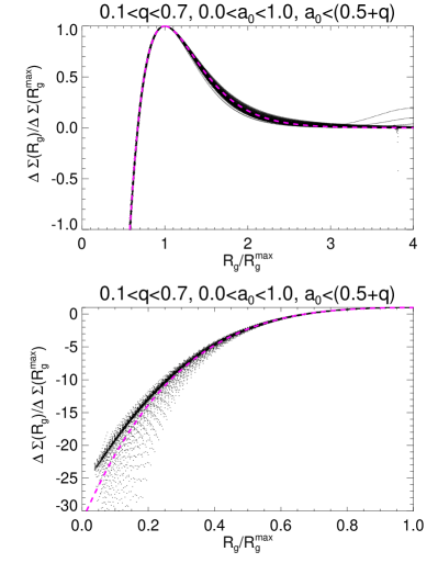
Figure 1.— The correction factor $\Delta\Sigma$ that is required to reproduce an exponential disc as a function of $R_{g}$. $R_{g}^{\rm max}$ is the radius at which $\Delta\Sigma$ is maximum. Different curves in the figure correspond to different values of $a_{0}$ and $q$. The magenta dashed lines correspond to an analytic fit. The bottom panel shows the same set of curves as the top panel but shows the region $0<R_{g}/R_{g}^{\rm max}<1$ in greater detail.

3.1. Case of $f_{\rm Shu}$ with a flat rotation curve

The correction factor $\Delta\Sigma$ as a function of $R_{g}$ for various different values of $a_{0}$ and $q$ is shown in LABEL:f1. In general, we find that $\Delta\Sigma$ is negative for small $R_{g}$; it then rises to a maximum and then for large $R_{g}$ it asymptotically approaches zero (black lines in LABEL:f1). If there exists a unique functional form, then we must first reduce $\Delta\Sigma$ to a scale invariant form. To this end, we compute $s(R_{g}/R_{g}^{\rm max})=\Delta\Sigma(R_{g})/\Delta\Sigma(R_{g}^{\rm max})$, $R_{g}^{\rm max}$ being the value of $R_{g}$ where $\Delta\Sigma$ is maximum. In LABEL:f1, we plot $\Delta\Sigma(R_{g})/\Delta\Sigma(R_{g}^{\rm max})$ for various different values of $a_{0}$ and $q$ as derived by the iterative solution. It can be seen that they almost follow a unique functional form, except for $R_{g}/R_{g}^{\rm max}<0.2$, where slight differences can be seen (see lower panel LABEL:f1). Next we fit this by a function of the following form

$$s(x) = ke^{-x/b}((x/a)^{2}-1).$$ (30)

Imposing the condition that $x_{\rm max}=1$, $\int_{-\infty}^{\infty}xf(x)=0$ and $s(x^{\rm max})=1$, one can solve for $a,b$ and $k$. The final function is then given by

$$s(x) = 31.53e^{-x/0.2743}(x/0.6719)^{2}-1)$$ (31)

and this is plotted as magenta dashed lines in LABEL:f1. It can be seen that the proposed functional form provides a good fit. For greater accuracy one should replace this with a numerical function.

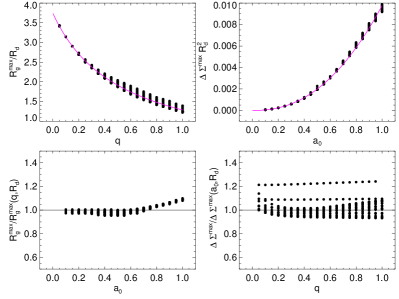
Figure 2.— The dependence of $R_{g}^{\rm max}$ and $\Delta\Sigma^{\rm max}$ on $q$ and $a_{0}$. The magenta lines are the fitted functional forms for $R_{g}^{\rm max}$ and $\Delta\Sigma^{\rm max}$. The bottom panels demonstrate that $R_{g}^{\rm max}$ and $\Delta\Sigma^{\rm max}$ are nearly independent of $a_{0}$ and $q$ respectively.

We now empirically determine the dependence of $R_{g}^{\rm max}$ and $\Delta\Sigma(R_{g}^{\rm max})$ on $R_{d},q$ and $a_{0}$ and this is given below.

$$R_{g}^{\rm max} = \frac{c_{1}}{1+q/c_{2}}R_{d}$$ (32)

$$\Delta\Sigma(R_{g}^{\rm max}) = \frac{1}{R_{d}^{2}}c_{3}a^{c_{4}}_{0}.$$ (33)

with $c_{1}=3.74$, $c_{2}=0.523$, $c_{3}=0.00976$, $c_{4}=2.29$,

It was found that the position of maximum $R_{g}^{\rm max}$ is mainly determined by $q$, while the amplitude $\Delta\Sigma(R_{g}^{\rm max})$ is mainly governed by $a_{0}$. In LABEL:f2, we plot $R_{g}^{\rm max}$ and $\Delta\Sigma(R_{g}^{\rm max})$ as functions of $q$ and $a_{0}$ respectively. The fitted functional forms Equation (32) and Equation (33) are shown as magenta lines. The bottom panel shows the dependence of $R_{g}^{\rm max}$ and $\Delta\Sigma(R_{g}^{\rm max})$ as a function of $a_{0}$ and $q$ respectively after dividing by the derived functional forms. It is clear that there is very little dependence of $R_{g}^{\rm max}$ on $a_{0}$ or of $\Delta\Sigma(R_{g}^{\rm max})$ on $q$.

The final functional form for $\Sigma(R_{g})$ can now be written as

$$\Sigma_{\rm corr}(R_{g}) = \frac{e^{-R_{g}/R_{d}}}{2\pi R_{d}^{2}}$$ (34)

$$-\frac{0.00976a^{2.29}_{0}}{R_{d}^{2}}s\left(\frac{R_{g}}{3.74R_{d}(1+q/0.523)}\right)$$

3.2. Case of $f_{\rm Shu}$ with a non-flat rotation curve

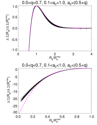
Figure 3.— The correction factor $\Delta\Sigma$ for distribution function $f_{\rm Shu}(E,L)$ with $v_{\rm circ}(R)=v_{c}(R/R_{d})^{0.2}$. For description see Figure1.

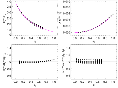
Figure 4.— The dependence of $R_{g}^{\rm max}$ and $\Delta\Sigma^{\rm max}$ on $q$ and $a_{0}$ for distribution function $f_{\rm Shu}(E,L)$ with $v_{\rm circ}(R)=v_{c}(R/R_{d})^{0.2}$. For description see Figure2.

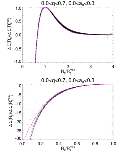
Figure 5.— The correction factor $\Delta\Sigma$ for distribution function $f_{\rm Shu}(E,L)$ with $v_{\rm circ}(R)=v_{c}\sqrt{1+R_{d}/R}$. For description see Figure1.

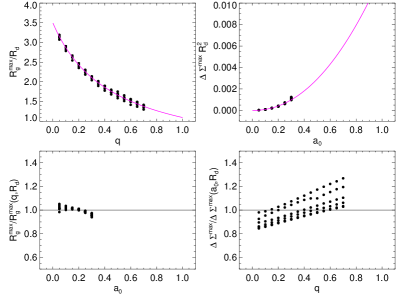
Figure 6.— The dependence of $R_{g}^{\rm max}$ and $\Delta\Sigma^{\rm max}$ on $q$ and $a_{0}$ for distribution function $f_{\rm Shu}(E,L)$ with $v_{\rm circ}(R)=v_{c}\sqrt{1+R_{d}/R}$. For description see Figure2.

We now repeat the same exercise for cases where the rotation curve is not flat. Specifically, we investigate the following two cases.

• Rising rotation curve: The circular velocity is assumed to be a power law with positive slope.

  $$v_{\rm circ}(R) = v_{c}(R/R_{d})^{\beta}\ {\rm with}\ \beta=0.2$$ (35)

  $$\phi(R) = v_{c}^{2}(R/R_{d})^{2\beta}/(2\beta)\ {\rm with}\ \beta=0.2$$ (36)

• Falling rotation curve: In this case we assume the potential to be a superposition of a point mass and a flat rotation curve. The circular velocity decreases monotonically with radius but at large $R$ asymptotes to a constant value.

  $$v_{\rm circ}(R) = v_{c}^{2}(1+\sqrt{R_{d}/R})$$ (37)

  $$\phi(R) = v_{c}^{2}(\log(R/R_{d})-R_{d}/R)$$ (38)

  It should be noted that we do not study the case of a rotation curve falling as a power law, as the integral of the Shu distribution function over all space or more specifically the factor $g_{K}(a,R_{g})$ becomes infinite.

The results for the above two rotation curves are shown in LABEL:f3, LABEL:f4, LABEL:f5 and LABEL:f6 and the fit parameters $c_{1},c_{2},c_{3}$ and $c_{4}$ are summarized in Table 1. It can be seen from LABEL:f3 and LABEL:f5 that the $\Delta\Sigma$ curves follow an almost universal form. The functional form differs only slightly from the case for a flat rotation curve. From LABEL:f4 and LABEL:f6, it can be seen that the functional form given by Equation (32) and Equation (33) provides a good fit for the dependence of $R_{g}^{\rm max}$ and $\Delta\Sigma^{\rm max}$ on $q$ and $a_{0}$ respectively. A slight residual dependence on $q$ of $\Delta\Sigma^{\rm max}$ is visible for falling rotation curve (lower right panel of LABEL:f6). If we ignore the dependence of parameters $c1,c2,c3,c4$ on the rotation curve, i.e., $\beta$, the resulting surface density profiles will be slightly inaccurate. For $(a0,q)=(0.5,0.33)$, comparing $\Sigma_{\rm corr}(R_{g})$ of $\beta=0$ with that of $\beta=0.2$, we find that maximum deviation occurs at around $R\sim R_{g}^{\rm max}$ and is about 10%.

3.3. Case of $f_{\rm Dehnen,a}$ with a flat rotation curve

Figure 7.— The correction factor $\Delta\Sigma$ for distribution function $f_{\rm Dehnen,a}(E,L)$ with $v_{\rm circ}(R)=v_{c}$. For description see Figure1.

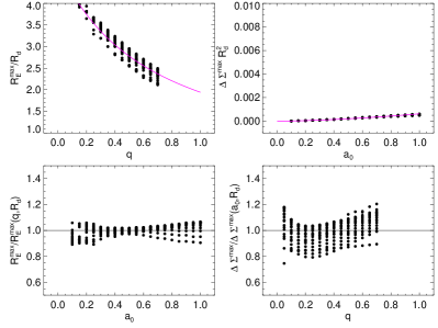
Figure 8.— The dependence of $R_{g}^{\rm max}$ and $\Delta\Sigma^{\rm max}$ on $q$ and $a_{0}$ for distribution function $f_{\rm Shu}(E,L)$ with $v_{\rm circ}(R)=v_{c}$. For description see Figure2.

Finally, we study the case of a distribution function different from Shu. We use the function $f_{\rm Dehnen,a}$ from Dehnen (1999). For this, we only study the case of a flat rotation curve. It can be seen from LABEL:f7 that the $\Delta\Sigma$ curves again follow an almost universal form. However, the form is different from that of $f_{\rm Shu}$. The main difference being that as $R_{E}$ approaches zero the curve moves upwards to large positive values. The functional form of $R_{E}^{\rm max}(q)$ and $\Delta\Sigma^{\rm max}(a_{0}))$ is the same as in $f_{\rm Shu}$ but with different values for constants, and the relationships are slightly less accurate than for $f_{\rm Shu}$ (see LABEL:f8). Interestingly, $\Delta\Sigma^{\rm max}$ is much smaller than the case for Shu distribution function.

To summarize, we find that for a given distribution function and rotation curve, the correction factor $\Sigma(R_{c})$ required to reproduce exponential discs for different values of $a_{0}$ and $q$ follows a universal functional form to high accuracy. The scale length $R_{c}^{\rm max}$ and the amplitude of this function $\Delta\Sigma^{\rm max}$ has a simple dependence on $a_{0}$ and $q$ which can be parameterized in terms of four constant $c_{1}$, $c_{2}$, $c_{3}$ and $c_{4}$. The fact that an empirical formula based on the above methodology can be determined for different rotation curves and even for a distribution function other than $f_{\rm Shu}$ is very promising. The reason that the methodology works for different cases is related somewhat to the following three facts

• The functional form of the required target density is same for all cases.

• We have parameterized the velocity dispersion in a way such that its dependence on $R_{c}$ is same for all cases.

• The integral equation governing the computation of $\Delta\Sigma$ is the same for all cases except for the Kernel function and its normalization function $g_{K}$.

Given an integral equation of the type in Equation (23), the determination of $\Sigma(R)$ from $\Sigma(R_{c})$ can be thought of as a convolution operation with a Kernel function $K(R,R_{c})$. To first order, if the kernels are similar and of the same width, the effect of convolution should be insensitive to the shape of the kernel. For the cases studied here the kernel in general peaks at $R=R_{c}$ and then falls of sharply for both $R<R_{c}$ and $R>R_{c}$. The exact shape is governed primarily by the form of the distribution function. For a constant rotation curve, the width of the kernel is an exponentially decreasing function of $R_{c}$. The effect of a non-flat rotation curve is to simply modulate this functional dependence of width as a function of $R_{c}$.

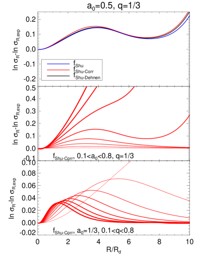
Figure 9.— The logarithmic difference of the radial velocity dispersion profile $\sigma_{R}(R)$ with respect to the target velocity dispersion profile $\sigma_{R,{\rm exp}}(R)=v_{c}a_{0}\exp(-qR/R_{d})$. In the top panel the three cases shown are for the Shu distribution function with flat rotation curve, a) without the empirical formula ($f_{\rm Shu}$) b) with the empirical formula ($f_{\rm Shu-Corr}$) c) with Dehnen’s ansatz ($f_{\rm Shu-Dehnen}$). The bottom two panels are for $f_{\rm Shu-Corr}$ only. Here the different lines correspond to different values of $a_{0}$ and $q$ and the thickness of the line is proportional to the value of $a_{0}$ and $q$. The values of $a_{0}$ and $q$ increase in steps of 0.1.

Figure 10.— The fractional difference of the surface density $\Sigma(R)$ from the target surface density for different choices of $\Sigma(R_{g})$. The target surface density $\Sigma_{\rm exp}={\rm exp}(-R/R_{d})/(2\pi R_{d}^{2})$ is that of an exponential disc. $\Sigma_{\rm corr}(R_{g})$ is the formula presented in this paper which approximately reproduces an exponential disc. Different lines correspond to different choices of $a_{0}$ and $q$. In the bottom panel $q$ is fixed and the thickness of the lines is proportional to the value of $a_{0}$.

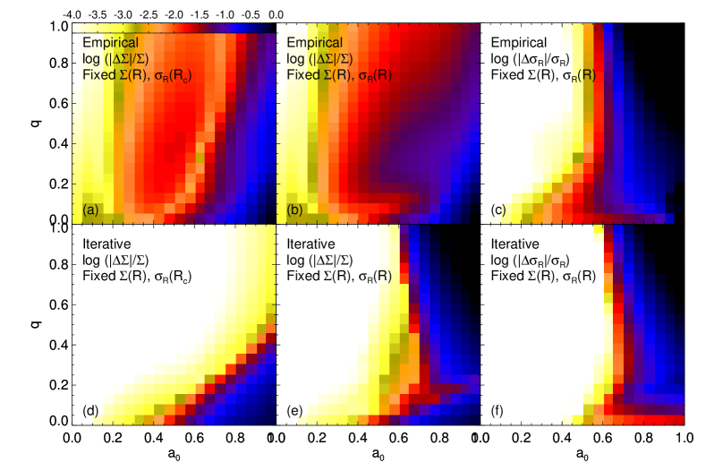
Figure 11.— The mean absolute fractional difference of the final surface density $\Sigma(R)$ and velocity dispersion $\sigma_{R}(R)$ from the target surface density $\exp(-R/R_{d})/(2\pi R_{d}^{2})$ and target velocity dispersion $v_{c}a_{0}\exp(-qR/R_{d})$. Shown is the case of $f_{\rm Shu}$ with flat rotation curve. The top panels are results from using the empirical formula proposed in this paper. The bottom panels are results from using the iterative algorithm. The panels a and d correspond to the case where $\Sigma(R)$ and $\sigma_{R}(R_{c})$ are specified to follow exponential functional forms. The other panels are for the case where $\Sigma(R)$ and $\sigma_{R}(R)$ are specified to follow exponential functional forms. The mean difference was computed over equi-spaced bins in $0<R/R_{d}<5$, and was not weighted for mass variation else the contribution to the mean from large values of $R$ would be very small.

3.4. The case of velocity dispersion profiles that are exponential in radius

Till now, we had assumed the $\sigma_{R}(R_{c})$ profile to be fixed and exponential in $R_{c}$. However, this does not result in $\sigma_{R}(R)$ profiles that are strictly exponential in radius $R$. For $f_{\rm Shu}$ with flat rotation curve, the deviation of $\sigma_{R}(R)$ from that of an exponential form $\sigma_{R}(R)=v_{c}a_{0}\exp(-qR/R_{d})$ is shown in top panel of LABEL:f9. The deviation is very similar to the deviation noticed for surface densities, so the effect can be thought of as an increase in scale length of the exponential function governing the radial dependence of the dispersion profile. The case of $f_{\rm Shu}$ both with and without the use of empirical formula result in very similar $\sigma_{R}(R)$ profiles. Additionally, a form of $f_{\rm Shu}$ with Dehnen’s ansatz (see Equation (40)) also gives a similar $\sigma_{R}(R)$ profiles. This suggests that modifying the $F(R_{c})$ part of the distribution function only has a minor effect on the dispersion profiles. The primary quantity that determines the dispersion profile is the function $\sigma_{R}(R_{c})$. It can be seen from LABEL:f9 that the difference peaks at around $R/R_{d}=4$ then decreases and finally for large $R$ it starts to rise again. The bottom panel of LABEL:f9 shows that the location of the peak primarily depends on $q$ (for small $q$, the peak is at larger $R$) while the height depends on both $a_{0}$ and $q$. The larger the $a_{0}$ and smaller the $q$, the higher the peak. The rise at large $R$ is mainly dependent on $a_{0}$ and is stronger for large $a_{0}$. This is because the distribution of guiding center $R_{g}$ in a given annulus at large $R$ is bimodal. The main peak being from stars with $R_{g}\sim R$ but there is also a secondary peak from stars with very small $R_{g}$. The secondary peak has a non-negligible contribution to the velocity dispersion as the corresponding $\sigma_{R}(R_{g})$ is very large due to the exponential functional dependence. Unlike us, this rise at large $R$ is not visible in Figure-1a of Dehnen (1999) and we believe that this is because in Dehnen (1999) the convolution integral is not done over the full domain of $R_{g}$ but instead only around $R_{g}\sim R$.

If one desires $\sigma_{R}(R)=v_{\rm circ}(R)a_{0}\exp(-qR/R_{d})$ then one has to use the Dehnen (1999) iterative solution to solve for both $\sigma_{R}(R_{c})$ and $\Sigma(R_{c})$ simultaneously. We do this for the case of $f_{\rm Shu}$ with flat rotation curve. Doing so, we find that the $\Sigma_{R}(R_{g})$ profile is almost unchanged from the case where $\sigma_{R}(R)$ was not constrained. For $\sigma_{R}(R_{g})$ we find that an empirical formula as given below can reproduce to a good accuracy the desired velocity dispersion profiles.

$$\sigma_{R}^{\rm corr}(R_{g}) = v_{c}a_{0}\exp(-qR_{g}/R_{d})\times$$ (39)

$$\left(1-\frac{0.25a_{0}^{2.04}}{q^{0.49}}f_{\rm poly}(R_{g}q/R_{d})\right),$$

Here $f_{\rm poly}$ is an 11 degree polynomial having coefficients- $0.028476$, $-1.4518$, $12.492$, $-21.842$, $19.130$, $-10.175$ , $3.5214$, $-0.81052$, $0.12311$, $-0.011851$, $0.00065476$, $-1.5809\times 10^{-5}$.

4. Accuracy in reproducing the target density

In the top panel of LABEL:f10, we plot the fractional difference of the final surface density $\Sigma(R)$, as compared to that of an exponential disc, using our empirical formula as given by Equation (34) for the case of $f_{\rm Shu}$ with flat rotation curve. Results for a range of values of $a_{0}$ and $q$ are shown. For $R/R_{d}<5$, the difference is less than $10\%$. The fit starts to deteriorate only for $R/R_{d}>5$. In general, as $a_{0}$ is increased, the fit progressively deteriorates. For comparison, the bottom panel shows the fractional difference of $\Sigma(R)$ when a simple exponential form for $\Sigma(R_{g})$ is adopted. The difference increases as $a_{0}$ is increased and is negligible only for very small values of $a_{0}$. The improvement offered by the empirical formula is clearly evident here.

The accuracy of the formula as a function of $a_{0}$ and $q$ can be better gauged in panels a and d of LABEL:f11 . Here we plot the mean absolute fractional difference of surface density $\Sigma(R)$ with respect to the target surface density $\Sigma_{\rm exp}(R)=\exp(-R/R_{d})/(2\pi R_{d}^{2})$ as a function of $a_{0}$ and $q$. It can be seen that the proposed solution works quite well over most of the $(a_{0},q)$ space except for very high values of $a_{0}$. It should be noted that in the region $a_{0}>q+0.5$, lower right corner, where the empirical formula fails the iterative solution also itself fails (see panel d). So the actual inaccuracy of the formula is mainly confined to the region $(q>0.4,a_{0}>0.75)$.

We now study the accuracy of our analytic formula given by Equation (34) and Equation (39) for the case where both the target surface density and the velocity dispersion are specified to follow exponential forms. The mean absolute fractional difference of $\Sigma(R)$ and $\sigma_{R}(R)$ with respect to $\Sigma(R)=\exp(-R/R_{d})/(2\pi R_{d}^{2})$ and $\sigma_{R}=v_{c}a_{0}\exp(-qR/R_{d})$ is shown in panels b and c of LABEL:f11. For comparison, the panels e and f show the results of the iterative algorithm. It can be seen that the formula works well in the range $0<a_{0}<0.5$, where the mean error is less than 1%. However for $a_{0}>0.5$, the formula and the iterative solution both do not work well. It should be noted that the sharp transition at $a_{0}\sim 0.5$ is due to the fact that we measure the difference over the range $0<R/R_{d}<5$. Extending the range would shift the transition value of $a_{0}$ to lower values and vice versa. In general, for a given $a_{0}$ the solution provided by the iterative method and the empirical formula are both accurate in reproducing target profiles for small values of $R$, they gradually become inaccurate at larger values of $R$. It can also be seen from the figure that for $a_{0}>0.5$, the empirical formula performs slightly better than the iterative solution at reproducing the target surface densities. However, this is only at the expense of not matching the target velocity dispersion profiles as well.

We now discuss the possible causes for the failure of the iterative solution for large $a_{0}$. The iterative algorithm will only work correctly if the contribution to the integral for $\Sigma(R)$ or $\sigma_{R}(R)$ (see Equation 23 and 24), is confined to a local region around $R_{c}\sim R$. In general, at large $R$ this condition is violated. The radius at which this violation occurs depends upon the choice of $a_{0}$, and is lower for larger values of $a_{0}$. This violation of the locality condition is stronger for $\sigma_{R}(R)$ profiles, as $\sigma_{R}(R_{c})$ increases exponentially with decrease in $R_{c}$. The rise in $\Delta\sigma_{R}/\sigma_{R}$ at large $R$ as discussed in Section 3.4 and LABEL:f9 is also a manifestation of this effect. This is the main reason that when the constraint of exponential radial dispersion profiles is applied the algorithm fails for $a_{0}>0.5$.

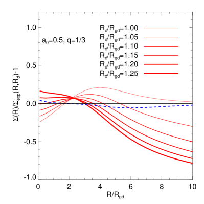
Figure 12.— The fractional difference of the surface density $\Sigma(R)$ from the target surface density, $\Sigma_{\rm exp}={\rm exp}(-R/R_{d})/(2\pi R_{d}^{2})$, for $\Sigma(R_{g})={\rm exp}(-R_{g}/R_{gd})/(2\pi R_{gd}^{2})$. The thickness of the line is proportional to the value of $R_{d}$ used for $\Sigma_{\rm exp}$. The dashed line is the result of using our empirical formula with $R_{gd}=R_{d}$.

4.1. Comparison with other approximate solutions

An alternative way to generate an exponential disc using a Shu type distribution function was proposed in Binney (2010). They note that the effect of warming up the distribution function is to expand the disc, and this can be thought of as an increase in scale length of the disc. So, one way to take this into account is to start with a slightly smaller scale length when specifying $\Sigma(R_{g})$. There are two problems with this approach. First, the factor by which the scale length will have to be reduced will depend upon the values of $a_{0}$ and $q$. So the solution is no simpler than what we propose. Secondly, we find that even if one has the correct factor, the solution is less than optimal. To show this, we plot in LABEL:f12 the fractional difference of the surface density $\Sigma(R)$ obtained using $\Sigma(R_{g})={\rm exp}(-R_{g}/R_{gd})/(2\pi(R_{gd})^{2})$ from an exponential surface density with different values of $R_{d}$. We set $a_{0}=0.5$ and $q=0.33$ which is typical of old thin disc stars. The case considered is that of $f_{\rm Shu}$ with flat rotation curve. It can be seen that increasing $R_{d}$ improves the solution slightly for $R/R_{gd}<5$, but at the expense of deteriorating it for large $R$. Overall, the quality of the fit is quite poor. For comparison, the dashed line is the result using our empirical formula with $R_{gd}=R_{d}$, which clearly performs better.

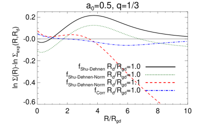
Figure 13.— The logarithmic difference of the surface density $\Sigma(R)$ from the target surface density, $\Sigma_{\rm exp}={\rm exp}(-R/R_{d})/(2\pi R_{d}^{2})$, for $\Sigma(R_{g})={\rm exp}(-R_{g}/R_{gd})/(2\pi R_{gd}^{2})$. Shown are the results for the Dehnen’s ansatz with different scale length. The results of our empirical formula are also shown alongside.

One might argue that the ansatz of Dehnen (1999)

$$f_{\rm Shu-Dehnen}(E,L)=\frac{\gamma(R_{g})\Sigma(R_{g})}{2\pi\sigma_{R}^{2}(R_{g})}\exp\left(\frac{E_{c}(R_{g})-E}{\sigma_{R}^{2}(R_{g})}\right)$$ (40)

actually produces discs that are more close to an exponential form, and so applying the Binney (2010) scale length reduction to it might produce even better agreement. We now investigate this issue. Firstly, the above distribution function is not normalized. If $\sigma_{R}(R_{g})$ is parameterized in terms $a_{0}$ and $q$ as before then it has a normalization that depends upon the choice of $a_{0}$ and $q$, so the full distribution function is not purely analytical anymore. On top of that as said earlier, the factor by which the scale length will have to be reduced will also depend upon the values of $a_{0}$ and $q$. We assume it to be 10% for the time being. In LABEL:f13, we show the fractional difference of surface density from the target density for the case of $f_{\rm Shu-Dehnen}$ with flat rotation curve. Results with normalization (denoted by $f_{\rm Shu-Dehnen-Norm}$) and with Binney (2010) scale length reduction are also shown alongside. It can be seen that after normalizing the Dehnen’s ansatz does produce discs that match the target density better, i.e., the range of deviation is smaller than the thin red line corresponding to $R_{g}/R_{d}=1$ in LABEL:f12. After applying the Binney (2010) scale length reduction the agreement gets even better, but only in regions with $R/R_{d}<4$. For large $R$, there is still a wide discrepancy. In comparison, it can be seen that the formula proposed in this paper (dashed blue line) is still superior while being simpler and fully analytic.

5. Discussion

In this paper, we have presented an empirical formula for Shu-type distribution functions which can reproduce with good accuracy a disc with an exponential surface density profile. This should be useful in constructing equilibrium N-body models of disc galaxies (Kuijken & Dubinski, 1995; McMillan & Dehnen, 2007; Widrow & Dubinski, 2005) where such functions are employed. It can also be employed in synthetic Milky Way modelling codes like TRILEGAL (Girardi et al., 2005), Galaxia (Sharma et al., 2011) and Besancon (Robin et al., 2003). Finally, the most important use of our new formalism is for MCMC fitting of theoretical models to large data sets, e.g., the Geneva-Copenhagen (Nordström et al., 2004) , RAVE (Steinmetz et al., 2006) and SEGUE stellar surveys (Yanny et al., 2009). Here, separable analytic approximations of this kind are required to make the problem tractable (Sharma et al 2013, in preparation).

One of our main finding is that the part of the distribution function that determines the target surface density can be written as the target density plus a correction term which approximately follows a unique functional form. So, the problem reduces to determining the scale and the amplitude of this correction function and their dependence on $a_{0}$ (ratio of central velocity dispersion to circular velocity) and $q$ (a parameter controlling the gradient of the dispersion as a function of radius). The problem is further simplified as we find that the scale is primarily a function of only $q$ and the amplitude is a primarily a function of only $a_{0}$. These findings are valid for not only flat rotation curves but also for cases with rising and falling rotation curves. Additionally, it was also found to be valid for one of the Dehnen (1999) distribution functions. An extension of the formula to reproduce velocity dispersion profiles that are exponential in radius was also found to work well. This suggests that the methodology presented can, in principle, be also applied to other disc distribution functions proposed by Dehnen (1999) and Binney (2010, 2012) which are conceptually similar.

Appendix A Integral equation for one of the Dehnen distribution functions

We consider here the distribution function

$$f_{\rm Dehnen,a} = \frac{F(R_{E})}{\sigma^{2}_{R}(R_{E})}\exp\left(-\frac{E-E_{c}(L)}{\sigma^{2}_{R}(R_{E})}\right)$$ (A1)

from Dehnen (1999). For $f_{\rm Dehnen,a}$ one can write the probability distribution in $(R,R_{E},R_{g})$ space as

$$P(R,R_{E},R_{g})dRdR_{E}dR_{g} = 2\pi f(E,L)dLdR2d|v_{R}|$$ (A2)

$$P(R,R_{E},R_{g}) = 2\pi f(E,L)\frac{dL}{dR_{g}}\frac{dE}{dR_{E}}\frac{2}{\sqrt{2(E-\Phi(R))-L^{2}/R^{2}}}$$ (A3)

To proceed further we assume a flat rotation curve. Using $E=\Phi_{\rm eff}(R_{E},R_{E})$, $E_{c}(R_{g})=\Phi_{\rm eff}(R_{g},R_{g})$, $dL/dR_{g}=\frac{2v_{\rm circ}(R_{g})}{\gamma^{2}(R_{g})}$, $dE/dR_{E}=\frac{2v_{\rm circ}^{2}(R_{E})}{\gamma^{2}(R_{E})R_{E}}$, $\gamma^{2}(R_{g})=\gamma^{2}(R_{E})=2$ we get

$$P(R,R_{E},R_{g}) = \frac{4\pi F(R_{E})}{a^{2}(R_{E})}\frac{R_{E}^{-(1+\frac{1}{a^{2}})}R_{g}^{\frac{1}{a^{2}}}}{\sqrt{1-2\ln(R/R_{E})-R_{g}^{2}/R^{2}}}$$ (A4)

Substituting $\frac{R_{g}}{R\sqrt{1-2\ln(R/R_{E})}}=x$ and

$$K(R,R_{E})=(R/R_{E})^{(1+\frac{1}{a^{2}})}(1-2\ln(R/R_{E}))^{\frac{1}{2a^{2}}}$$ (A5)

this simplifies to

$$P(R,R_{E},x) = \frac{4\pi F(R_{E})}{a^{2}(R_{E})}K(R,R_{E})\frac{x^{\frac{1}{a^{2}}}}{\sqrt{1-x^{2}}}$$ (A6)

Integrating over $x$ from 0 to 1 we get

$$P(R,R_{E}) = \frac{4\pi F(R_{E})}{a^{2}(R_{E})}K(R,R_{E})h(a)$$ (A7)

where

$$h(a)=\int_{0}^{1}\frac{x^{1/a^{2}}}{\sqrt{1-x^{2}}}=\frac{\sqrt{\pi}}{2}\frac{\Gamma(\frac{1}{2a^{2}}+\frac{1}{2})}{\Gamma(\frac{1}{2a^{2}}+1)}=\frac{\sqrt{\pi}}{2}\frac{\Gamma(c+\frac{1}{2})}{\Gamma(c+1)}\ {\rm with}\ c=\frac{1}{2a^{2}}$$ (A8)

Using $\int P(R,R_{E})dR=2\pi R_{E}\Sigma(R_{E})$ one can write $F(R_{E})$ in terms of $\Sigma(R_{E})$ to get

$$F(R_{E}) = \frac{\Sigma(R_{E})a^{2}(R_{E})}{2g_{K}(a)h(a)}$$ (A9)

and then

$$P(R,R_{E}) = \frac{2\pi\Sigma(R_{E})}{g_{K}(a)}K(R,R_{E})$$ (A10)

Here

$$g_{K}(a) = \frac{1}{R_{E}}\int K(R,R_{E})dR=\left(\frac{e}{1+c}\right)^{1+c}\frac{\Gamma(1+c)}{2}\ {\rm with}\ c=\frac{1}{2a^{2}}$$

$$\approx \sqrt{\frac{\pi}{2(c+1)}}\ {\rm for\ large\ c}.$$

References

- Binney (2010) Binney, J. 2010, MNRAS, 401, 2318
- Binney (2012) —. 2012, MNRAS, 426, 1328
- Binney & McMillan (2011) Binney, J., & McMillan, P. 2011, MNRAS, 413, 1889
- Dehnen (1999) Dehnen, W. 1999, AJ, 118, 1201
- Girardi et al. (2005) Girardi, L., Groenewegen, M. A. T., Hatziminaoglou, E., & da Costa, L. 2005, A&A, 436, 895
- Kalnajs (1976) Kalnajs, A. J. 1976, ApJ, 205, 751
- Kuijken & Dubinski (1995) Kuijken, K., & Dubinski, J. 1995, MNRAS, 277, 1341
- McMillan & Binney (2012) McMillan, P. J., & Binney, J. 2012, MNRAS, 419, 2251
- McMillan & Dehnen (2007) McMillan, P. J., & Dehnen, W. 2007, MNRAS, 378, 541
- Nordström et al. (2004) Nordström, B., et al. 2004, A&A, 418, 989
- Robin et al. (2003) Robin, A. C., Reylé, C., Derrière, S., & Picaud, S. 2003, A&A, 409, 523
- Sandage (1969) Sandage, A. 1969, ApJ, 158, 1115
- Schönrich & Binney (2009) Schönrich, R., & Binney, J. 2009, MNRAS, 396, 203
- Schönrich & Binney (2012) —. 2012, MNRAS, 419, 1546
- Sharma et al. (2011) Sharma, S., Bland-Hawthorn, J., Johnston, K. V., & Binney, J. 2011, ApJ, 730, 3
- Shu (1969) Shu, F. H. 1969, ApJ, 158, 505
- Steinmetz et al. (2006) Steinmetz, M., et al. 2006, AJ, 132, 1645
- van der Kruit & Searle (1982) van der Kruit, P. C., & Searle, L. 1982, A&A, 110, 61
- Widrow & Dubinski (2005) Widrow, L. M., & Dubinski, J. 2005, ApJ, 631, 838
- Yanny et al. (2009) Yanny, B., et al. 2009, AJ, 137, 4377