Dynamical signatures of infall around galaxy clusters: a generalized Jeans equation

Abstract

We study the internal kinematics of galaxy clusters in the region beyond the sphere of virialization. Galaxies around a virialized cluster are infalling towards the cluster centre with a non-zero mean radial velocity. We develop a new formalism for describing the dynamical state of clusters, by generalizing the standard Jeans formalism with the inclusion of the peculiar infall motions of galaxies and the Hubble expansion as well as the contributions due to background cosmology. Using empirical fits to the radial profiles of density, mean radial velocity and velocity anisotropy of both a stacked cluster-mass halo and two isolated haloes of a cosmological dark matter only simulation, we verify that our generalized Jeans equation correctly predicts the radial velocity dispersion out to 4 virial radii. We find that the radial velocity dispersion inferred from the standard Jeans equation is accurate up to 2 virial radii, but overestimated by $\approx 20\%$ for the stacked halo and by $\approx 40\%$ for the isolated haloes, in the range $\approx 2-3$ virial radii. Our model depends on the logarithmic growth rate of the virial radius (function of halo mass or concentration), which we estimate in 7 different ways, and on the departure from self-similarity of the evolution of the peculiar velocity profile in virial units.

1 Introduction

Galaxy clusters are the largest gravitationally bound structures in the Universe. Cluster studies represent a particularly deep source of information in modern cosmology, since they provide constraints on the growth of structures in the Universe and on cosmological parameters, in particular the dark energy equation of state parameter $w$, from the evolution of the cluster mass function (Haiman et al., 2001; Voit, 2005; Cunha et al., 2009). A crucial role is played by the accuracy to which we can determine the cluster mass. Therefore, the estimation of the cluster total mass has become an important research field, which still remains a demanding task, mainly because most of the matter content in clusters is not visible.

Clusters are characterized by a virialized region within which all components (galaxies, intracluster medium and dark matter) are in rough dynamical equilibrium, where galaxy motions are well described by the Jeans formalism.

The cluster mass distribution can be measured through many complementary methods. The first approach to the cluster mass determination was the application of the virial theorem to the member galaxies (Zwicky, 1933). More sophisticated techniques are based on the hydrostatic measure of X-ray emissivity and temperature of the hot cluster gas (Ettori et al., 2002; Borgani et al., 2004; Zappacosta et al., 2006; Schmidt & Allen, 2007; Host & Hansen, 2011), on the analysis of large-scale velocity field (Mohayaee & Tully, 2005) and on the analysis of the galaxy motions in clusters through the Jeans formalism. The radial profiles of total mass and velocity anisotropy of clusters have been constrained by Jeans analysis in several ways: predicting the observed radial profile of the line-of-sight velocity dispersion (Girardi et al., 1998), as well as kurtosis (Łokas & Mamon, 2003; Łokas et al., 2006); by isotropic (Katgert et al., 2004) or anisotropic mass inversion (Mamon & Boué, 2010). Alternative methods to use galaxy motions, are by fitting the $\Lambda$CDM distribution function (Wojtak et al., 2008) to the distribution of galaxies in projected phase-space density (Wojtak et al., 2009; Wojtak & Łokas, 2010) or by applying the caustic technique (Diaferio, 1999).

Observations (Rines & Diaferio, 2006), N-body simulations (Mamon et al., 2004; Wojtak et al., 2005; Cuesta et al., 2008) and a combination of both (Mahajan et al., 2011) have shown that virialized clusters are surrounded by infall zones from which most galaxies move into the relaxed cluster, as predicted by Gunn & Gott (1972). These galaxies are gravitationally bound to the cluster but are not fully virialized. This picture sparks multiple questions: does the infall motion affect the standard formalism? Can we detect the effect of the infall in cluster observations? Can this detection help to constrain the total mass of clusters? Below we will attempt to answer some of these questions.

The dynamical and X-ray based mass estimators depend on the hypothesis that the cluster is in steady-state dynamical or hydrostatic (for X-rays) equilibrium. The presence of non-stationary motions just outside the virial sphere may invalidate this assumption at that scale. For example, the standard Jeans formalism involves outward integration along the line of sight, beyond the virial radius, hence into the regions with negative mean radial velocities, which are not accounted for. Moreover, the Jeans analysis relies on the assumption that the mean matter density of the Universe does not contribute to the gravitational potential (the so-called Jeans swindle), and does not take into account the effect of the expansion of the Universe. Therefore, the mass estimated through the usual methods may be significantly biased and not be the true dynamical mass of the cluster. Two additional methods have been developed to address this issue: gravitational lensing (e.g. Mandelbaum et al., 2010; Lombriser, 2011), and the caustic technique (Diaferio, 1999; Serra et al., 2011), which are both independent of the dynamical state of the system. Zu & Weinberg (2013) developed also a novel technique for constraining the radial profiles of the infall velocity from the projected velocity distributions of galaxies around clusters.

The aim of this paper is to generalize the standard Jeans formalism to include radial streaming motions (i.e. infall), as well as cosmological terms. This leads to a more general Jeans equation that also describes the outer cluster region and simplifies to the standard Jeans equation when the infall and cosmological corrections are negligible, like inside the virial radius. Our motivation is to build a formalism with this generalized Jeans equation to measure more accurately the mass profiles of clusters beyond the virial radius. In Section 2, we develop the formalism of the generalized Jeans equation. We analyse a cosmological simulation in Section 3 to show that our generalized Jeans equation correctly reproduces the radial velocity dispersion, and we determine the bias on the velocity dispersion obtained with the standard Jeans equation.

2 Non-equilibrium dynamics of galaxy clusters: the generalized Jeans equation

The lowest-order Jeans equation relates the gravitational potential $\Phi$ of the cluster to the dynamical properties of the galaxies. In spherical coordinates, the standard Jeans equation is (e.g., Binney & Mamon, 1982)

$$-\rho(r)\frac{{\rm d}\Phi}{{\rm d}r} = -\rho(r)\frac{GM(r)}{r^{2}}$$ (1)

$$= \frac{{\rm d}(\rho\sigma_{r}^{2})}{{\rm d}r}+2\,\frac{\beta}{r}\,\rho\sigma_{r}^{2}\,.$$

Here $\rho(r)$ is the density distribution of a tracer (e.g., the number density of galaxies in and around clusters), $M(r)$ is the total mass distribution (including dark matter) in the cluster, $\sigma_{r}(r)$ is the galaxy velocity dispersion along the radial direction and $\beta(r)$ is the velocity anisotropy parameter defined by

$$\beta(r)=1-\frac{\sigma_{\rm\theta}^{2}(r)+\sigma_{\rm\phi}^{2}(r)}{2\sigma_{r}^{2}(r)}\,,$$ (2)

where $\sigma_{\rm\theta}(r)$ and $\sigma_{\rm\phi}(r)$ are the longitudinal and azimuthal velocity dispersions (and are equal by spherical symmetry). The anisotropy parameter expresses the cluster’s degree of radial velocity anisotropy. The value of $\beta$ can vary from $\beta=-\infty$, corresponding to circular orbits ($\sigma_{r}=0$), to $\beta=1$, if orbits are perfectly radial ($\sigma_{\rm\theta}=\sigma_{\rm\phi}=0$). When $\sigma_{\rm\theta}=\sigma_{\rm\phi}=\sigma_{r}$ the system is isotropic ($\beta=0$).

In equation (1), we neglect streaming motions and any time-dependence, i.e. the mean velocity components $\overline{v}_{\rm i}$ are identically zero and, therefore, the velocity dispersions correspond to the second moment of the velocity components $\sigma_{\rm i}^{2}=\overline{v_{\rm i}^{2}}$  .

We now wish to go beyond the stationary approximation and to take into account the possible presence of an infall motion of galaxies outside the virialized core of clusters.

When we include the galaxies with mean radial velocity $\overline{v}_{r}\neq 0$ and retaining time derivatives, the Jeans equation (obtained by taking the first velocity moment of the collisionless Boltzmann equation) becomes

$$-\rho\frac{{\rm d}\Phi}{{\rm d}r}=\frac{\partial(\rho\overline{v_{r}^{2}})}{\partial r}+\frac{\rho}{r}\left[2\,\overline{v_{r}^{2}}-(\overline{v_{\rm\theta}^{2}}+\overline{v_{\rm\phi}^{2}})\right]+\frac{\partial(\rho\overline{v}_{r})}{\partial t}\,.$$ (3)

The second-order velocity moment for the radial component is now related to the radial velocity dispersion $\sigma_{r}$ and the first velocity moment, i.e. the mean radial velocity $\overline{v_{r}}$, by the general expression

$$\overline{v_{r}^{2}}=\sigma_{r}^{2}+\overline{v_{r}}^{2}\,.$$ (4)

We keep $\overline{v_{\rm\theta}^{2}}=\sigma_{\rm\theta}^{2}$ and $\overline{v_{\rm\phi}^{2}}=\sigma_{\rm\phi}^{2}$, since we still assume no net longitudinal and azimuthal motions, i.e. we ignore bulk meridional circulation and rotation. Using the continuity equation

$$\frac{\partial\rho}{\partial t}=-\frac{\partial(\rho\overline{v}_{r})}{\partial r}-\frac{2}{r}\,\rho\overline{v}_{r}\,,$$ (5)

the Jeans equation (3) can be put in the following form:

$$-\rho\frac{{\rm d}\Phi}{{\rm d}r} = \frac{\partial(\rho\sigma_{r}^{2})}{\partial r}+2\,\frac{\beta}{r}\rho\sigma_{r}^{2}+\rho\left[\overline{v}_{r}\frac{\partial\overline{v}_{r}}{\partial r}+\frac{\partial\overline{v}_{r}}{\partial t}\right]\,.$$ (6)

Therefore, the inclusion of non-equilibrated material leads to a modification in the dynamical terms on the r.h.s. of the standard Jeans equation (1), namely to the addition of two extra terms involving the mean radial motion of galaxies. This correction is negligible in the virialized core of the cluster, but it can become significant in the outer region.

Since we are now considering distances very far from the centre of the cluster, we also need to take into account effects due to the underlying cosmology, meaning that the gravitational term in the Jeans equation also needs to be modified. The galaxies are subject to an attractive potential from the mean density of the background and a repulsive potential from the cosmological constant, and when we add these contributions, the potential gradient is given by

$$\frac{{\rm d}\Phi}{{\rm d}r}=\frac{GM(r)}{r^{2}}+\frac{4\pi}{3}G\rho_{b}r-\frac{1}{3}\Lambda r\,.$$ (7)

Here $\rho_{b}$ is the mean density of the Universe, $\Lambda$ the cosmological constant and $H=\dot{a}/a$ the Hubble constant. Introducing the dimensionless density parameter and cosmological constant commonly used

$$\Omega_{\rm m}=\frac{8\pi G\rho_{b}}{3H^{2}},\quad\Omega_{\Lambda}=\frac{\Lambda}{3H^{2}}\,,$$ (8)

equation (7) reads

$$\frac{{\rm d}\Phi}{{\rm d}r}=\frac{GM(r)}{r^{2}}+qH^{2}r\,,$$ (9)

in terms of the deceleration parameter:

$$q=-{\ddot{a}a\over\dot{a}^{2}}={\Omega_{\rm m}\over 2}-\Omega_{\Lambda}\,.$$ (10)

In general, the radial velocity of galaxies can be written as the sum of the Hubble flow and a peculiar (infall) velocity flow:

$$\overline{v}_{r}(r,t)=H(t)\,r+\overline{v}_{p}(r,t)\,,$$ (11)

and beyond the infall region surrounding the clusters, the peculiar velocity becomes negligible compared to the Hubble expansion:

$$\overline{v}_{r}(r,t)\approx H(t)\,r\quad\text{when}\quad r\to\infty\,.$$

One can now compute the non-stationary terms in equation (6) using equation (11)

$$\overline{v}_{r}\frac{\partial\overline{v}_{r}}{\partial r}+\frac{\partial\overline{v}_{r}}{\partial t}=\overline{v}_{p}\frac{\partial\overline{v}_{p}}{\partial r}+H\left(\overline{v}_{p}+r\,\frac{\partial\overline{v}_{p}}{\partial r}\right)-qH^{2}r+\frac{\partial\overline{v}_{p}}{\partial t}\,,$$ (12)

where we have written the time derivative of the Hubble parameter in terms of equation (10) :

$$\dot{H}=-(q+1)\,H^{2}\,.$$ (13)

Inserting equations (9) and (12) into equation (6), we obtain the generalized Jeans equation

$$\frac{\partial(\rho\sigma_{r}^{2})}{\partial r}+2\,\frac{\beta}{r}\rho\sigma_{r}^{2}=-\rho\left[\frac{GM(r)}{r^{2}}+S(r,t)\right]\,.$$ (14)

Here $\rho$ is the density of tracer. In this work, when applying the generalized Jeans equation to test haloes, we will consider only the particles belonging to the selected halo as our tracer. The mass $M(r)$ is thus the test halo mass, without the contribution from other haloes or the diffuse Universe.

Equation (14) differs from equation (1) by the inclusion of the new term

$$S(r,t) = q\,H^{2}r+\left(v_{r}{\partial v_{r}\over\partial r}+{\partial v_{r}\over\partial t}\right)$$ (15)

$$= \overline{v}_{p}\frac{\partial\overline{v}_{p}}{\partial r}+H\left(\overline{v}_{p}+r\,\frac{\partial\overline{v}_{p}}{\partial r}\right)+\frac{\partial\overline{v}_{p}}{\partial t}\,.$$ (16)

Equations (14) and (16) extend the standard Jeans formalism to describe also the non-stationary dynamics of clusters, and in principle, hold at any radius.

In equation (16), the background density and the cosmological constant contributions to the gravitational potential, cancel exactly with the velocity term relative to the pure Hubble flow. Thus, including all the effects due to the underlying cosmology corresponds to applying the Jeans swindle (Falco et al., 2013).

Therefore, the extra term $S(r,t)$ differs from zero only in the presence of infall velocity, i.e. setting $v_{p}(r,t)=0$, we immediately recover the standard Jeans equation (1).

The most general solution of equation (14) provides the following expression for the radial velocity dispersion profile, depending on $\rho(r)$, $M(r)$, $\beta(r)$ and $\overline{v}_{p}(r,t)$

$$\sigma_{r}^{2}(r) = \frac{1}{\rho(r)}\,\exp\left[-2\int_{0}^{r}\frac{\beta(s)}{s}\,{\rm d}s\right]$$ (17)

$$\times\,\int_{r}^{\infty}\exp\left[2\int_{0}^{s}\frac{\beta(\tilde{s})}{\tilde{s}}\,{\rm d}\tilde{s}\right]$$

$$\qquad\quad\times\,\rho(s)\,\left[\frac{GM(s)}{s^{2}}+S(s,t)\right]{\rm d}s\,,$$

using equation (16) for $S(s,t)$.

3 Comparison with cosmological simulations

3.1 The simulation

We analyse an N-body simulation with Wilkinson Microwave Anisotropy Probe 3 (WMAP3) cosmological parameters, $\Omega_{\rm m}=0.24$, ${\Omega_{\Lambda}}=0.76$, the dimensionless Hubble parameter $h=0.73$, the spectral index of primordial density perturbations $n=0.96$ and the power spectrum normalization $\sigma_{8}=0.76$. A box of size $160\,h^{-1}$Mpc and $1024^{3}$ particles was used. Starting from a redshift $z=30$, the evolution was followed using the message passing interface (MPI) version of the Adaptive Refinement Tree (ART) code. A hierarchical friends-of-friends (FOF) algorithm was used for identifying clusters. The linking length was $b=0.17$ times the mean inter-particle distance, corresponding roughly to an overdensity relative to the mean of the Universe of $\Delta=(1.96/b^{3})\,[\ln(c+1)-c/(c+1)]\,(1+c)^{2}/c^{2}\simeq 549\,(c/5)^{0.39}/(b/0.17)^{3}$ (adapted from More et al., 2011), where $c$ is the concentration parameter, for haloes with a NFW density profile (Navarro et al., 1996). We define the virial radius of our haloes as the radius of overdensity $\Delta=387$ (i.e. overdensity of $\Delta_{\rm c}=92.8$ relative to the critical density of the Universe) appropriate for the cosmology of the simulation (with the approximation of Bryan & Norman, 1998).

In order to test the generalized Jeans equation, which includes the effect of the infall motion, we shall look at cosmological simulations of clusters, and we demonstrate how to reproduce their radial velocity dispersions for radii larger than the virial radius. To this end, we first need to choose functions to parametrize the density, the mass, the anisotropy parameter and the infall velocity of the simulation to handle them as analytical functions in equations (16) and (17).

3.2 Analytical approximations to density, anisotropy and mean radial velocity profiles

N-body simulations show that the density distribution of a dark matter halo, in the inner virialized region, is well described by a double power-law profile (Kravtsov et al., 1998)

$$\rho_{\rm h}(r)=\frac{\rho_{s}}{\left(r/r_{\rm s}\right)^{\eta}\left(1+r/r_{\rm s}\right)^{\xi}}\,.$$ (18)

Here $r_{\rm s}$ is the scale radius, $\rho_{s}$ is the scale density, $\eta$ and $\xi$ are the slopes, with values close to 1 and 2 respectively, which correspond to the NFW model.

According to cosmological dark matter simulations (e.g. Mamon & Łokas, 2005 and references therein), the radial anisotropy typically varies from ($\approx 0-0.1$) at $r\approx 0$, increasing with the distance and reaching a maximum value ($\approx 0.3-0.8$) around one to two times the virial radius. Looking at larger radii, $\beta(r)$ also shows an almost universal trend: it drops to negative values, reaching a minimum, and then it approaches zero asymptotically (Wojtak et al., 2005; Ascasibar & Gottlöber, 2008). If we define $r_{0}$ as the radius at which $\beta(r)$ passes through zero before becoming negative, we can parametrize the anisotropy function as

$$\beta(r)=A\left(\frac{r}{r_{\rm v}}\right)^{\mu}\left(\frac{r_{0}-r}{r_{\rm v}}\right)\left[1+B\Bigl{(}\frac{r}{r_{\rm v}}\Bigr{)}^{\nu}\right]^{-\chi}\,,$$ (19)

where $r_{\rm v}$ is the virial radius.

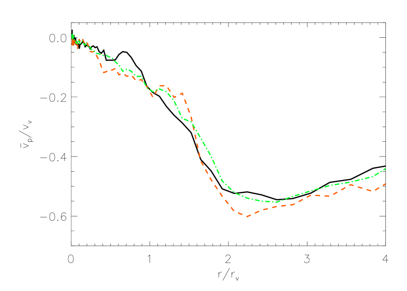
Figure 1: Mean peculiar radial velocity of three samples of stacked haloes. The mass ranges for the samples are: a very narrow mass range around $5\times 10^{13}\,M_{\odot}$ (green dot-dashed line), $(0.78-1.00)\times 10^{14}\,M_{\odot}$ (black, solid line) and $(1.00-1.27)\times 10^{14}\,M_{\odot}$ (red dashed line).

The new formalism also includes the mean infall velocity of galaxies as an additional unknown function. Simulations show a quite universal trend for the radial profile of the mean velocity up to very large radii. Fig. 1 displays the mean radial velocity with the Hubble flow subtracted, i.e. the peculiar component $\overline{v}_{p}$, up to 4 virial radii, for three samples of stacked halos. The samples contain the same number of haloes and the mass ranges are: a very narrow bin around $5\times 10^{13}\,M_{\odot}$ (green dot-dashed line), $(0.78-1.00)\times 10^{14}\,M_{\odot}$ (black, solid line) and $(1.4-1.8)\times 10^{14}\,M_{\odot}$ (red dashed line). The velocity is negative everywhere, clearly showing the infall motion, particularly pronounced between $\approx 1$ and $4\,r_{\rm v}$. The three profiles appear to look very similar.

In the innermost region, the cluster is fully equilibrated ($\overline{v}_{\rm r}=0$). The peculiar velocity profile can then be approximated, for $r\ll r_{\rm v}$, as

$$\overline{v}_{p}(r,t)\approx-H\,r\quad\,.$$ (20)

In general, the mean peculiar velocity can be written as

$$\overline{v}_{p}(r,t)=-H(t)\,r_{\rm v}(t)\,f\left(\frac{r}{r_{\rm v}(t)}\right)\ ,$$ (21)

where $f({r}/{r_{\rm v}})$ must be such that the condition  (20) is satisfied. As we will show in the next sections, the function $f\left({r}/{r_{\rm v}}\right)$ is well approximated by the formula

$$f\left(\frac{r}{r_{\rm v}}\right)=\left\{\left[\left(\frac{r}{r_{\rm v}}\right)^{-a}+C\left(\frac{r}{r_{\rm v}}\right)^{b}\right]^{1/a}-D\right\}^{-1}\,.$$ (22)

Equation (16) involves the time derivative of the radial infall velocity. Equations (21) and  (22) describe a profile where the dependence on time is through $H(t)$ and $r_{\rm v}(t)$. The function that describes the radial shape of the velocity, equation (22), might change in time as well. We parametrize this dependence by multiplying equation (21) by a factor that involves time only:

$$\overline{v}_{p}(r,t)=-H(t)\,r_{\rm v}(t)\,f\left(\frac{r}{r_{\rm v}(t)}\right)\,\left({t\over t_{0}}\right)^{\alpha}\ ,$$ (23)

where $t_{0}$ is the present age of the Universe.

We can now explicitly calculate the time derivative of $v_{p}(r)$ and complete the computation of the extra term $S(r,t)$, which then obeys

$${t\,S(r,t)\over v_{p}(r,t)} = H\,t\,\left[1+{{\rm d}\ln f\over{\rm d}\ln x}-{{\rm d}f\over{\rm d}x}\,\left({t\over t_{0}}\right)^{\alpha}\right]$$ (24)

$$\quad+{{\rm d}\ln H\over{\rm d}\ln t}+{{\rm d}\ln r_{\rm v}\over{\rm d}\ln t}\,\left(1-{{\rm d}\ln f\over{\rm d}\ln x}\right)+\alpha\ ,$$

where $x=r/r_{\rm v}$.

The parameter $\alpha$ describing the departure from self-similarity of the evolution of the infall velocity profile in virial units is not well known. In Appendix A, we analyse fig. 13c of Cuesta et al. (2008), describing this evolution for stacked haloes, to deduce that $\alpha\approx-0.55\pm 0.1$ (see Fig, 7). Since we are analysing our simulation at $z=0$, the precise value of $\alpha$ probably depends on the radial shape of the velocity at the present time. We consider it as a free parameter of our model, and we expect it to vary with a small scatter, when considering different velocity profiles.

In Appendix B, we estimate ${\rm d}\ln r_{\rm v}/{\rm d}\ln t$ using the mass growth rates measured in cosmological simulations as well as through analytical theory, to conclude that the mean growth of haloes at $z=0$ for the cosmology of our simulation and for the halo mean mass and concentration parameter is ${\rm d}\ln r_{\rm v}/{\rm d}\ln t\simeq 0.7$. We note that observers will tend to discard clusters having undergone recent mergers, while we stack 27 haloes regardless of their recent merger history, so that observers will effectively choose halos with slightly smaller values of ${\rm d}\ln r_{\rm v}/{\rm d}\ln t$. But in Appendix B, we also compute the minimal growth of a fully isolated halo in an expanding universe, and find ${\rm d}\ln r_{\rm v}/{\rm d}\ln t\simeq 0.68$, which is only very slightly lower.

Having expressions for $\rho$, $M$, $\beta$ and $\overline{v}$, we can then use equation (17) to calculate the radial velocity dispersion of simulated haloes, which we can compare to the true dispersion profile. In the next sections, we show the results obtained for a sample of stacked haloes and for two isolated haloes.

3.3 Comparison with a stacked halo

We begin by selecting a sample of 27 stacked cluster-size haloes from our simulation, with virial masses in the range $[(0.78-1.0)\times 10^{14}\,\rm M_{\odot}]$. We denote this sample as our stacked halo. The characteristic quantities of the stacked halo are taken as the mean of the 27 individual haloes, and are listed in Table 1.

Table 1: Virial parameters and concentrations of the haloes.

	$M_{\rm v}\ (10^{13}\,M_{\odot})$	$r_{\rm v}\ (\rm Mpc)$	$v_{\rm v}\ (\rm km\,s^{-1})$	$c$
Stacked	8.6	1.14	569	6.4
Halo 1	8.4	1.13	566	6.9
Halo 2	7.8	1.10	553	7.6

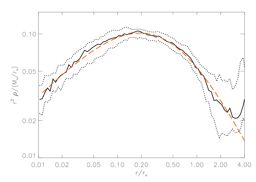
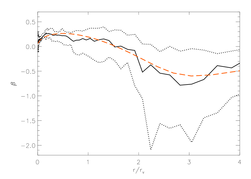
Figure 2: Density and anisotropy profiles of the stacked halo. Top panel: comparison between the quantity $r^{2}\rho(r)$, where $\rho(r)$ is the median density profile, from the simulation (black solid line), and from the parametric fit, with $\rho(r)$ given by equation (18) and best parameters listed in Table 2 (red dashed line). The black dotted lines denote the quartiles. Bottom panel: median (black solid) and quartiles (black dotted) velocity anisotropy profile. The red dashed line shows the fitting function (19) with parameters quoted in Table 2.

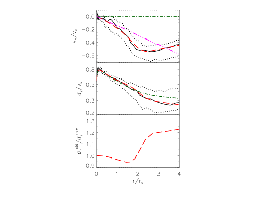
Figure 3: Mean peculiar radial velocity and radial velocity dispersion of the stacked halo. Top panel: median (solid black) and quartiles (dotted black) of the mean peculiar radial velocity profile measured in the simulation, and a fit to the form in equation (21) with parameters quoted in Table 2 (red dashed line). The green dash-dotted line represents the case of zero peculiar velocity. The magenta triple-dot-dashed line corresponds to the inner limit $\overline{v}_{p}\approx-Hr$ for $r\ll r_{\rm v}$. Middle panel: comparison between the radial velocity dispersion profile of the stacked halo, measured in spherical shells (black solid line), and the one computed by equation (17), where $\rho(r)$, $\beta(r)$ and $\overline{v}_{p}(r)$ are approximated with equations (18), (19) and (21), with the parameters of Table 2 (red dashed line). We set $\alpha=-1.0$ in equation (24). The green dash-dotted line shows the velocity dispersion profile from the standard Jeans equation (1), i.e. for zero mean peculiar velocity. The black dotted lines represent the quartiles. Bottom panel: ratio between the dispersion calculated with the standard Jeans equation (the green dash-dotted line in the middle panel) and with our new generalized equation (the red dashed line in the middle panel).

Fig. 2 shows the profiles of $r^{2}\rho(r)$ (top panel) and $\beta(r)$ (bottom panel) for the stacked halo. The black solid lines denote the median profiles from the simulation, the black dotted lines correspond to the first and the third quartiles, and the red dashed lines represent our fits.

The density can be well approximated in the region ($r<3\,r_{\rm v}$) using the double-power formula of equation (18) , with parameters listed in Table 2. The simulated density profile increases beyond a turn-around radius of $3-4\,r_{\rm v}$, due to the presence of other structures surrounding the halo. Our model describes an isolated system; therefore, we do not take into account the presence of other structures.

The anisotropy profile is well fitted by equation (19) up to $4\,r_{\rm v}$. In our case, $r_{0}=1.55\,r_{\rm v}$, and the other best-fitting parameters for the anisotropy are listed in Table 2.

According to equation (17), the radial velocity dispersion also requires the knowledge of the mean peculiar radial velocity profile of the sample. In the upper panel of Fig. 3 are displayed the mean peculiar velocity of our sample (black solid line), quartiles (black dotted lines), and $\overline{v}_{p}(r)$ given by formula (21), with parameters listed in Table 2 (red dashed line). The green dash-dotted line represents the case of zero peculiar velocity.

The radial velocity dispersion is shown in the central panel of Fig. 3. The black solid line shows the simulated profile and the black dotted lines correspond to the first and the third quartiles. The green dash-dotted line shows the velocity dispersion profile from the standard Jeans equation (1). We compute the velocity dispersion by using equation (17) where the extra term is given by equation (24) and best parameters in Table 2 (red dashed line). We find that the best solution is given by setting $\alpha=-1$. This value of $\alpha$ is more negative than the value of $\approx-0.55\pm 0.1$ that we infer (Fig. 7) from the evolution of the stacked cluster-mass halo of Cuesta et al. (2008).

Table 2: Parameters of empirical fits to $\rho(r)$ (with eq. [18]), $\beta(r)$ (with eq. [19]) and $v_{p}(r)$ (with eq. [21]) for the stacked haloes.

$\rho(r)$	$\beta(r)$	$v_{p}(r)$
$\rho_{s}=2.4\,M_{\rm v}/r^{3}_{\rm v}$	$\mu=0.48$	$a=9.7$
$r_{s}=0.38\,r_{\rm v}$	$\nu=9.5$	$b=2.8$
$\eta=1.35$	$\chi=0.37$	$C=5.7\times\,10^{-5}$
$\xi=1.96$	$A=0.35$	$D=0.214$
	$B=5\times 10^{-5}$

The radial velocity dispersion profile measured for the halo matches very well the one predicted by our generalized Jeans equation (17) all the way out to $4\,r_{\rm v}$. The standard Jeans formalism can predict $\sigma_{r}$ up to $\approx 2\,r_{\rm v}$, where the infall and the cosmological corrections are still very small or cancel out. In the region where these contributions are significant the radial velocity dispersion inferred from equation (1) is overestimated by $\approx 20\%$ in the range $\approx 2-3$ virial radii, as shown in the bottom panel of Fig. 3. The slope of $\sigma_{r}$ becomes steeper in the region of non-equilibrium, and this is well reproduced by equation (17).

In Appendix C, we also present the results of the simulations at slightly larger radii, and consider relations between parameters of interest, in particular we show the derivative of the density, $\gamma$, and of the radial velocity dispersion, $\kappa$. We also present plots in the two-dimensional spaces $\gamma-\kappa$ and $\gamma-\beta$ for distances up to $\approx 6r_{\rm v}$.

3.4 Comparison with isolated haloes

The example in the previous section demonstrates the correctness of this generalized formalism when applied to a stacked sample of cluster-size haloes. However, when taking the median profiles of the stacked sample, we are not guaranteed that the individual halos will have the same profiles. Our median quantities based upon a sample with an odd number of haloes effectively correspond to a single halo. However, the halo involved in the median density at a given radius, may not be the same as that involved in the median radial velocity, or that for the median velocity anisotropy.

A further test is therefore to apply the same approach also to individual haloes in the sample, in order to be independent of the analysis of the median profiles. Our model describes the dynamics of clusters when they are isolated. Thus, we need to look for haloes in our sample which are not surrounded by massive neighbours. In particular, we have searched for haloes which have no neighbours with mass at least half of theirs, within a distance of $10\,r_{\rm v}$. With this criterion, we have selected two optimal haloes among the 27 belonging to our sample. We denote our haloes as halo 1 and halo 2. The virial masses, radii, velocities as well as their concentrations are listed in Table 1.

Table 3: Parameters of empirical fits to $\rho(r)$ (with eq. [18]), $\beta(r)$ (with eq. [19]) and $v_{p}(r)$ (with eq. [21]) for halo 1 and halo 2.

	$\rho(r)$	$\beta(r)$	$v_{p}(r)$
halo 1	$\rho_{s}=2.45\,M_{\rm v}/r^{3}_{\rm v}$	$\mu_{\rm inner}=0.5$	$a=4.75$
	$r_{s}=0.4\,r_{\rm v}$	$\mu_{\rm outer}=2.0$	$b=2.5$
	$\eta=1.37$	$\nu=23.0$	$C=4.8\times\,10^{-3}$
	$\xi=2.22$	$\chi=0.23$	$D=0.29$
		$A=0.6$
		$B=6\times 10^{-11}$
halo 2	$\rho_{s}=41\,M_{\rm v}/r^{3}_{\rm v}$	$\mu_{\rm inner}=0.57$	$a=4.8$
	$r_{s}=0.11\,r_{\rm v}$	$\mu_{\rm outer}=2.0$	$b=2.6$
	$\eta=0.9$	$\nu=24.6$	$C=2.4\times\,10^{-3}$
	$\xi=2.1$	$\chi=0.25$	$D=0.21$
		$A=0.5$
		$B=2.1\times 10^{-11}$

Fig. 4 shows the profiles of $r^{2}\rho(r)$ (top panels) and $\beta(r)$ (bottom panels) for the two individual haloes. We fit the profiles with, respectively, equations (18) for the density and (19) for the anisotropy. In the outer region, where the anisotropy takes negative values, the profiles of both haloes are much steeper than the median profile of the stacked halo. Therefore, in equation (19) it is convenient to use two different slopes: $\mu_{\rm inner}$ for $r<r_{0}$ and $\mu_{\rm outer}$ for $r>r_{0}$. For both haloes, $r_{0}=1.75\,r_{\rm v}$. The best-fitting parameters are shown in Table 3.

The infall velocity profiles of the haloes are displayed in the upper panels of Fig. (5). The corresponding radial velocity dispersion profiles are shown in the middle panels. The black solid lines denote the simulated profiles, and the red dashed lines correspond to the solution of equation (17), in the case of $v_{p}(r)$ given by our fits. We find that the value $\alpha=-0.65$ provides a good match to the velocity dispersion for both haloes. The green dash-dotted lines denote the velocity dispersion profiles from the standard Jeans equation (1).

Also in the case of these two isolated haloes, we find that our prediction of the velocity dispersion matches very well the measured profiles. The standard Jeans solution provides a good match up to $\approx\,2\,r_{\rm v}$, while our generalized Jeans equation improves the match at distances $\approx 2-4\,r_{\rm v}$.

The bottom panels of Fig. 5 show the ratio between the standard Jeans solution and our generalized solution. For the isolated haloes, the ratio is slightly larger than the one computed for the stacked sample. The velocity dispersion calculated by the standard Jeans equation is overestimated by $\approx 40\%-60\%$ for the first halo and $\approx 40\%$ for the second halo, in the range $\approx 2-4$ virial radii.

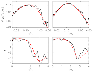
Figure 4: Density and anisotropy profiles of the isolated haloes. The left-hand panels correspond to halo 1 and the right-hand panels correspond to halo 2. Top panels: comparison between the quantity $r^{2}\rho(r)$, where $\rho(r)$ is the radial density profile, from the simulation (black solid line), and from the parametric fit, with $\rho(r)$ given by equation (18) and best parameters listed in Table 3 (red dashed line). Bottom panels: radial velocity anisotropy profile (black solid line). The red dashed line shows the fitting function (19) with parameters quoted in Table 3.

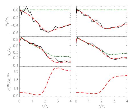
Figure 5: Mean peculiar radial velocity and radial velocity dispersion of the isolated haloes. The left-hand panels correspond to halo 1 and the right-hand panels correspond to halo 2. Top panels: mean peculiar radial velocity profile measured in the simulation (black solid line), and a fit to the form in equation (21) with parameters quoted in Table 3 (red dashed line). The green dashed-dotted line represents the case of zero peculiar velocity. Middle panels: comparison between the radial velocity dispersion profile, measured in spherical shells (black solid line) and the ones computed by equation (17), where $\rho(r)$, $\beta(r)$ and $\overline{v}_{p}(r)$ are approximated with equations (18), (19) and (21), with the parameters of Table 3 (red dashed line). For both haloes, we set $\alpha=-0.65$ in equation (24). The green dash-dotted line corresponds to the velocity dispersion profile from the standard Jeans equation (1), i.e. for zero mean peculiar velocity. Bottom panels: Ratio between the dispersion calculated with the standard Jeans equation (the green dash-dotted line in the middle panel) and with our new generalized equation (the red dashed line in the middle panel).

Instead of considering $\sigma_{r}$ for given mass and anisotropy profiles, one can estimate the error in the mass profile derived from the standard Jeans equation (1), relative to that derived from the generalized Jeans equation, for given $\sigma_{r}(r)$ and $\beta(r)$. Comparing with the standard and generalized Jeans equations, one finds that the mass derived from the standard Jeans equation (1) can be written as

$$M_{\rm std-Jeans}(r)=\left[1+{S(r)\over GM(r)/r^{2}}\right]\,M(r)\ ,$$ (25)

where $M(r)$ is the mass profile obtained from the generalized Jeans equation. Fig. 6 shows that beyond the virial radius, the corrections to the standard Jeans equation (1) are not negligible: in the range $\approx 2-4\,r_{\rm v}$, the correction causes the standard Jeans equation to underestimate the total mass by $\approx 20-60\%$ for halo 1 and $\approx 20-40\%$ for halo 2.

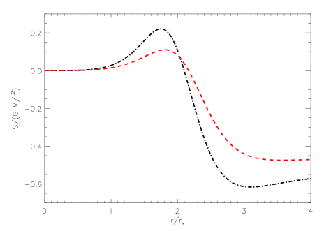
Figure 6: Relative mass excess deduced from the standard Jeans equation (1), relative to that from the generalized Jeans equation (14). The curves show the predictions using the parameters that we fit for halo 1 (black dot-dashed) and halo 2 (red dashed).

4 Conclusions and Discussion

The general purpose of this work is to improve our understanding of the dynamics of galaxies that are still falling on to relaxed clusters, with the motivation of performing a Jeans analysis of the mass profile out to several virial radii, for possible cosmological applications. The standard Jeans equation describing the cluster dynamics, assumes the system to be in equilibrium, with no mean radial streaming motions, and therefore it cannot be applied beyond the fully virialized cluster zone.

We have presented a generalized Jeans equation that takes into account the non-zero mean radial velocities of galaxies outside the virial radius, as well as the background density and the cosmological constant terms. We accurately reproduce the radial velocity dispersion profiles of a stack of 27 cluster-mass haloes and of two isolated haloes, out to 4 virial radii. In particular, while the standard Jeans equation provides accurate radial velocity dispersions out to $\approx 2$ virial radii, it over estimates the radial velocity dispersion by typically a factor 1.5 beyond $\approx 3$ virial radii. In the standard Jeans formalism, the total mass is underestimated by $\approx\,20-60\%$ in the region $\approx 2-4\,r_{\rm v}$.

A consistent description of cluster dynamics in the infall region can be useful for an accurate dynamical mass measurement at the infall scale. The estimation of mass profiles with the standard Jeans analysis involves the modelling of the line-of-sight velocity dispersion of the tracer (i.e. galaxies in clusters) by solving the lowest-order Jeans equation, to compare with that obtained from taking the second moments of the observed galaxy line of sight velocities. This also involves a measurement of the radial velocity anisotropy of galaxies. Just as several approaches have been proposed to break the mass velocity anisotropy degeneracy inherent to the standard Jeans equations, we wish to do the same when applying the generalized Jeans equation all the way to several virial radii, except that we also need to determine a third quantity : the mean infall velocity. As our parametrized approach to recover the radial velocity dispersion profile beyond the virial radius requires 12 free parameters, it should be viewed more as a proof of concept that the standard Jeans equation is adequate for determining the radial velocity dispersion profile up to 2 virial radii and inadequate beyond, rather than being a method to accurately determine the radial velocity dispersion profile from observational data. Karachentsev & Nasonova (2010) recover the infall pattern of the Virgo cluster, with the knowledge of the depth along the line of sight obtained from distance indicators independent of redshift (Mei et al., 2007). However, the uncertainties on the velocities appear to be too large for reproducing the radial velocity dispersion profile more accurately with the generalized Jeans equation than with the standard Jeans equation.

The model also involves the logarithmic growth rate of the virial radius as well as the departure from self-similarity of the evolution of the infall velocity profile. We have presented seven theoretical derivations for the logarithmic growth rate of the virial radius (as a function of mass or concentration), which lead to similar values. On the other hand, our stacked halo leads to a different non-self-similarity parameter ($\alpha$) than our two isolated haloes. We suspect that this parameter is not universal, but strongly depends on the mass accretion history of the halo. It would be useful to analyse the non-self-similarity parameter in more detail with simulations.

We finally note that with infall present, the kinetic energy is expected to be larger than in the case with no infall. The virial ratio, $2K/W=1$, can be seen as a spatial integral over the Jeans equation, where $K$ and $W$ represent the total kinetic energy and the total potential energy of the system. One therefore expects the virial ratio to be larger than unity for systems where infall is important (Cole & Lacey, 1996; Power et al., 2012).

We are planning an extension of this work to test how far the standard Jeans equation is relevant in reproducing the line-of-sight velocity dispersion profile and possibly find signatures of infall in the shape of the line-of-sight velocity profile.

Appendix A Departure from self-similarity of the evolution of the peculiar velocity

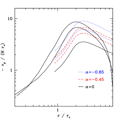
Figure 7: Time evolution of the mean peculiar velocity profile (in virial units). The black curves show the peculiar velocity measured in simulations at $z=0$, 1, and 2 (going upwards at $r=2\,r_{\rm v}$), adapted from fig. 13c of Cuesta et al. (2008). The red and blue curves show the predictions for $z=1$ and 2 obtained by extrapolating the $z=0$ curve with $(t/t_{0})^{\alpha}$. Two values of $\alpha$ are shown: one ($\alpha=-0.65$) that matches best the maximum absolute value of the peculiar velocity and one ($\alpha=-0.45$) that represents a best compromise over the relevant range of radii.

Cuesta et al. (2008) have measured the mean radial infall velocity as a function of radius, averaging over haloes of different mass, and repeating the exercise at $z=0$, 1 and 2. Their fig. 13c shows that the infall pattern is not self-similar, but instead decreases in time (in virial units). We converted their mean radial velocity to peculiar velocity (subtracting the Hubble flow). Fig. 7 shows that the evolution of the mean peculiar velocity in virial units is not self-similar: the black curves do not lie on top of one another. Assuming that $v_{p}(r,t)/[H(t)r_{\rm v}(t)]$ scales as $(t/t_{0})^{\alpha}$ improves the self-similarity. The peak peculiar velocities are reproduced for $\alpha=-0.65$, but the absolute peculiar velocities at large radii are overpredicted. Choosing $\alpha=-0.45$ represents a good compromise over the range of radii that are relevant: those where we measure the radial velocity dispersion and those slightly beyond that take part in the outwards integration of equation (14).

Appendix B Growth rate of the virial radius

There are several ways to compute the logarithmic growth rate of the virial radius, ${\rm d}\ln r_{\rm v}/{\rm d}\ln t$.

B.1 Self-similar growth in Einstein de Sitter universe

For a single halo in a universe with present-day density and dark energy parameters $\Omega_{m}=1$ and $\Omega_{\Lambda}=0$, one simply has ${\rm d}\ln r_{\rm v}/{\rm d}\ln t=8/9\simeq 0.89$, independent of the halo mass (Gunn & Gott, 1972).

B.2 Exponential halo mass evolution with redshift

Wechsler et al. (2002) analysed cosmological simulations and derived $M_{\rm v}(z)=M(z=0)\,\exp(-\alpha z)$, with $\alpha\approx 0.6$ for haloes of mass close to those considered here ($M\approx 8\times 10^{13}M_{\odot}$). With

$$M_{v}={\Delta\over 2}\,{H^{2}\,r_{\rm v}^{3}\over G}\ ,$$ (26)

this yields

$${{\rm d}\ln r_{\rm v}\over{\rm d}\ln t}={1\over 3}\,\left({{\rm d}\ln M_{v}\over{\rm d}\ln t}-{{\rm d}\ln\Delta\over{\rm d}\ln t}-2{{\rm d}\ln H\over{\rm d}\ln t}\right)\ .$$ (27)

One can write ${\rm d}\ln M_{\rm v}/{\rm d}\ln t=-\alpha/({\rm d}\ln t/{\rm d}z)$. Given that, for a flat universe, one has (Peebles, 1993, equation 13.20)

$$H_{0}\,t(z)={2\over 3\,\sqrt{1-\Omega_{\rm m}}}\,\sinh^{-1}\left({\sqrt{(1/\Omega_{\rm m})-1}\over(1+z)^{3/2}}\right)\ ,$$ (28)

one finds

$$\left({{\rm d}\ln t\over{\rm d}z}\right)_{z=0}=-{3\over 2}\,{\sqrt{1-\Omega_{\rm m}}\over\sinh^{-1}\sqrt{1/\Omega_{\rm m}-1}}\ ,$$ (29)

which tends to $-0.975$ for the density parameter of our simulation, $\Omega_{\rm m}=0.24$. We deduce that ${\rm d}\ln M_{\rm v}/{\rm d}\ln t\simeq 0.615$.

Given that, for a flat universe, one also has (Peebles, 1993, equation 13.3)

$$E(z)={H(z)\over H_{0}}=\sqrt{\Omega_{\rm m}(1+z)^{3}+1-\Omega_{\rm m}}\ ,$$ (30)

one deduces

$${{\rm d}\ln H\over{\rm d}\ln t} \!\!\!\!=\!\!\!\! -{\Omega_{\rm m}\over\sqrt{1-\Omega_{\rm m}}}\,(1+z)^{3}\,{\sqrt{1-\Omega_{\rm m}\left[1-(1+z)^{3}\right]}\over 1+\Omega_{\rm m}z\left(3+3z+z^{2}\right)}\sinh^{-1}\left({\sqrt{1/\Omega_{\rm m}-1}\over(1+z)^{3/2}}\right)$$ (31)

$$\!\!\!\!=\!\!\!\! -{\Omega_{\rm m}\over 1-\Omega_{\rm m}}\,\sinh^{-1}\left(\sqrt{1/\Omega_{\rm m}-1}\right)\qquad(z=0)\ ,$$

$$\!\!\!\!\simeq\!\!\!\! -0.402-1.08\,(\Omega_{\rm m}\!-\!0.27)-[0.638+0.698\,(\Omega_{\rm m}\!-\!0.27)]\,z\ ,$$ (32)

where the approximation is from a series expansion and is accurate to better than 1.7% (0.7% rms) for $0<z<0.2$ and $0.24<\Omega_{\rm m}<0.3$. So for our case of $\Omega_{\rm m}=0.24$ and $z=0$, equation (31) yields ${\rm d}\ln H/{\rm d}\ln t\simeq-0.37$.

Finally, using the approximation (Bryan & Norman, 1998)

$$\Delta\simeq 18\,\pi^{2}+82\,[\Omega_{m}(z)-1]-39\,[\Omega_{m}(z)-1]^{2}$$ (33)

where

$$\Omega_{\rm m}(z)={\Omega_{\rm m}\,(1+z)^{3}\over E^{2}(z)}$$ (34)

(see eq. [30]), we find the series expansion

$${{\rm d}\ln\Delta\over{\rm d}\ln t}\simeq-0.841+0.570\,(\Omega_{\rm m}-0.27)+[0.337+5.47\,(\Omega_{\rm m}-0.27)]\,z+[1.447-6.01\,(\Omega_{\rm m}-0.27)]\,z^{2}\ ,$$ (35)

which is accurate to better than 2.4% (0.9% rms) for $0<z<0.2$ and $0.24<\Omega_{\rm m}<0.3$. For $\Omega_{\rm m}=0.24$ and $z=0$, equation (35) yields ${\rm d}\ln\Delta/{\rm d}\ln t\simeq-0.85$. Putting this altogether, we deduce that ${\rm d}\ln r_{\rm v}/{\rm d}\ln t\simeq 0.735$.

B.3 Scaling with inverse Hubble time

Zhao et al. (2003) noted that $r_{\rm v}\propto 1/H$. With ${\rm d}\ln H/{\rm d}\ln t\simeq-0.37$ (Section B.2), we obtain ${\rm d}\ln r_{\rm v}/{\rm d}\ln t\simeq 0.37$ for the Zhao et al. approximation.

B.4 Constant circular velocity

Mamon et al. (2012) noted that the mean growth of haloes follows roughly $v_{\rm circ}(r_{\rm v})=\rm const$. Equation (26) then implies that $r_{\rm v}\propto 1/(H\sqrt{\Delta})$. With ${\rm d}\ln H/{\rm d}\ln t\simeq-0.37$ and ${\rm d}\ln\Delta/{\rm d}\ln t\simeq-0.85$ (Section B.2), we derive ${\rm d}\ln r_{\rm v}/{\rm d}\ln t\simeq 0.795$ for the constant circular velocity approximation, close to the $\Omega_{\rm m}=1$ slope, but far from the slope with the Zhao et al. approximation.

B.5 Halo merger rate in Millennium simulations

Fakhouri et al. (2010) have measured the halo merger rate in the Millennium and Millennium-II cosmological dark matter simulations. Their equation (2) provides the mean and median mass growth rates as ${\rm d}M_{v}/dt=a\,(M_{v}/10^{12}M_{\odot})^{1.1}(1+b\,z)E(z)$, with $a=46$ (mean) or 25 (median) $M_{\odot}\,\rm yr^{-1}$ and $b=1.11$ (mean) or 1.65 (median). Hence,

$${{\rm d}\ln M_{v}\over{\rm d}\ln t}={a\over 10^{12}}\,t(z)\,\left({M_{v}\over 10^{12}M_{\odot}}\right)^{0.1}(1+b\,z)\,E(z)\ ,$$ (36)

where $t(z)$ is measured in yr. The (slightly) positive slope on mass recovers the fact that high-mass haloes are rare today and even rarer in the past, and must therefore grow faster. Combining with equation (26), one obtains

$${{\rm d}\ln r_{\rm v}\over{\rm d}\ln t} \simeq 0.548+0.00511\,{a\over h}+\left(0.530-0.005\,{a\over h}\right)\,(\Omega_{\rm m}\!-\!0.27)$$ (37)

$$\qquad+\left[0.426-0.00308\,{a\over h}\,(1-1.66\,b)\right]\,z+0.00118\,{a\over h}\,(\log M\!-\!14)\ .$$

Equation (37) is accurate to 4% (1.4% rms) for $0<z<0.2$, $0.24<\Omega_{m}<0.3$, and $12<\log M/M_{\odot}<15.4$. Equations (27) and (36) yield ${\rm d}\ln r_{\rm v}/{\rm d}\ln t\simeq 0.74$, 0.79, 0.86, and 0.95 (mean) or 0.64, 0.67, 0.71 and 0.76 (median) for $\Omega_{\rm m}=0.24$, $h=0.73$, $z=0$, and $\log M$ = 12, 13, 14, and 15, respectively.

B.6 Extended Press-Schechter theory

Neistein & Dekel (2008) use extended Press-Schechter theory to derive a mass growth rate that can be written as ${\rm d}\ln M_{v}/{\rm d}\ln t=-\alpha\,t\,\dot{\omega}\,(M/10^{12}M_{\odot})^{\beta}$ with $\dot{\omega}\simeq-0.047\,[1+z+0.1\,(1+z)^{-1.25}]^{2.5}\,(h/0.73)\,\rm Gyr^{-1}$, $\alpha=0.59$ and $\beta=0.141$. With equations (30), (27), and (35), this leads to the series expansion

$${{\rm d}\ln r_{\rm v}\over{\rm d}\ln t} \simeq 0.548+0.264\,\alpha\,10^{2\beta}+\left(0.530-0.268\,\alpha\,10^{2\beta}\right)\,(\Omega_{m}-0.27)$$ (38)

$$\qquad+\left(0.426+0.259\,\alpha\,10^{2\beta}\right)\,z+0.607\,\alpha\,\beta\,10^{2\beta}\,(\log M\!-\!14)\ .$$

Equation (38) is good to 7.6% (2.4% rms) accuracy in the range $0<z<0.2,0.24<\Omega_{\rm m}<0.3,12<\log M/M_{\odot}<15.4$. The exact solution yields ${\rm d}\ln r_{\rm v}/{\rm d}\ln t=0.69$, 0.75, 0.84, and 0.96 for $z=0$, $\Omega_{\rm m}=0.24$, and $\log M=12$, 13, 14 and 15, respectively.

B.7 Minimum growth rate

We can estimate a minimum growth rate by considering the growth of a single halo in a uniform universe. Assuming an NFW density profile at all times, with mass profile

$$M(r,t) = M(a)\,\widetilde{M}\left({r\over a}\right)$$ (39)

$$\widetilde{M}\left({r\over a}\right) = {\ln(x+1)-x/(x+1)\over\ln 2-1/2}\ ,$$ (40)

where $a$ is the radius of slope $-2$ and does not vary in time. The virial radius $r_{\rm v}$ is the solution to

$${3\,M(r,t)/\left(4\pi\,r^{3}\right)\over 3\,H^{2}(t)/8\pi\,G}=\Delta(t)$$ (41)

i.e., using equation (40),

$${2\,G\,M(a)\over a^{3}}\,{\widetilde{M}(c)\over c^{3}}=\Delta(t)\,H^{2}(t)\ ,$$ (42)

where $c=r_{\rm v}/a$ is the concentration parameter. Now we do not need to solve equation (42) for $c$ to obtain the growth rate of $r_{\rm v}$. Indeed, at time $t+dt$, where $dt\ll t$, equation (42) becomes

$${2\,G\,M(a)\over a^{3}}\,{\widetilde{M}(c)\over c^{3}}\,\left[1+\left({{\rm d}\ln\widetilde{M}\over{\rm d}\ln x}\right)_{x=c}\,{dc\over c}-3\,{dc\over c}\right]=\Delta(t)\,H^{2}(t)+{{\rm d}\left(\Delta\,H^{2}\right)\over{\rm d}\ln t}\,{\rm d}\ln t\ .$$ (43)

Dividing equation (43) by equation (42), one obtains

$${{\rm d}\ln r_{\rm v}\over{\rm d}\ln t}={{\rm d}\ln c\over{\rm d}\ln t}={({\rm d}\ln\Delta/{\rm d}\ln t)+2\,({\rm d}\ln H/{\rm d}\ln t)\over({\rm d}\ln\widetilde{M}/{\rm d}\ln x)_{x=c}-3}\ .$$ (44)

After a series expansion, equation (44) becomes

$${{\rm d}\ln r_{\rm v}\over{\rm d}\ln t}\simeq 0.723+0.413\,z+0.698\,(\Omega_{\rm m}-0.27)-0.207\,(\log c-0.7)-1.79\,(\Omega_{\rm m}-0.27)\,z\ .$$ (45)

The approximation of equation (45) is accurate to 3.7% (1.4% rms) for $0<z<0.2$, $0.24<\Omega_{\rm m}<0.3$, and $0.5<\log c<1$. For $\Omega_{\rm m}=0.24$ and $z=0$, equation (44) yields ${\rm d}\ln r_{\rm v}/{\rm d}\ln t=0.75$, 0.70, 0.67, and 0.65 for $c=3$, 5, 7, and 10, respectively. One therefore notices that Zhao et al.’s approximation of $r_{\rm v}\propto 1/H$ yields a slower growth rate for $r_{\rm v}$ than our minimum growth rate found here. Note that, for $\Omega_{\rm m}=1$ and $z=0$, the minimum growth rate is ${\rm d}\ln r_{\rm v}/{\rm d}\ln t\simeq 0.879+0.252\,(\log c-0.7)$, not far from the Einstein de Sitter universe growth rate (Gunn & Gott, 1972, see Section B.1), with equality for $c=4.57$.

B.8 Summary

In summary, for the cosmology of our simulation, at $z=0$ for our mean halo mass of $8.6\times 10^{13}M_{\odot}$ and concentration parameter $c=6.4$, we find ${\rm d}\ln r_{\rm v}/{\rm d}\ln t=0.86$ (from Fakhouri et al.’s analysis of the merger rate in the Millennium simulations), 0.795 (for our constant circular velocity approximation), 0.735 (from Wechsler et al. et al’s exponential mass growth), 0.71 (from Neistein & Dekel’s extended Press-Schechter theory), 0.68 for the minimal growth scenario, but only 0.37 for Zhao et al.’s scaling with inverse Hubble time. We consider this last scaling as inaccurate and we adopt ${\rm d}\ln r_{\rm v}/{\rm d}\ln t=0.7$, slightly above our minimal growth scenario.

Appendix C Relations between slopes

Various numerical simulations have identified a range of apparent universalities, where some are identified in cosmological simulations, and others are found in controlled simulations. Most of these universalities are usually considered in radial ranges where the systems are fully equilibrated. Since we are considering here radial ranges much beyond the virial radius, it is relevant to study these properties at large radii.

Probably the most famous universality is the density profile as a function of mass (Navarro et al., 1996). It suggests that the density slope

$$\gamma=\frac{{\rm d}\log\rho}{{\rm d}\log r}$$ (46)

has a smooth transition from $-1$ in the inner region, to $-3$ in the outer region. The corresponding plot is shown for the stacked clusters in Fig. 8. It is clearly seen that around the virial radius the density profile flattens out, and the logarithmic slope approaches $-1$ around three times the virial radius. The green line shows the prediction for the double slope profile with parameters in Table 2.

Fig. 9 shows the relation between $\gamma$ and the velocity dispersion anisotropy given by equation (2). This is quite in agreement with the universality proposed in (Hansen & Stadel, 2003)

$$\beta=-0.2\,(\gamma+0.8)$$ (47)

in the inner region, but departs significantly for $\gamma<-2.2$.

A connection between $\gamma$ and the radial velocity dispersion was suggested by (Taylor & Navarro, 2001; Ludlow et al., 2011)

$$\frac{\rho}{\sigma^{3}}\approx r^{-\alpha},$$ (48)

where $\alpha=1.875$, in agreement with the prediction from the spherical infall model (Bertschinger, 1985). In Fig. 10 the derivative of the velocity dispersion is displayed:

$$\kappa=\frac{{\rm d}\log\sigma_{r}^{2}}{{\rm d}\log r}.$$ (49)

Equation (48) in terms of $\kappa$ and $\gamma$ reads

$$\gamma=-\alpha+\frac{3}{2}\kappa\ .$$ (50)

The connection in the $\gamma-\kappa$ space is in fair agreement with the formula (50), as we show in Fig. 11.

Figure 8: Logarithmic derivative of the density profile $\gamma$ (equation 46). Starting from $\gamma\approx-1$, the slope of the density function decreases reaching $\approx-3.2$ at around two times the virial radius, and in the outer region it increases again approaching zero. The green line shows the prediction for the double slope profile with parameters in Table  2

.

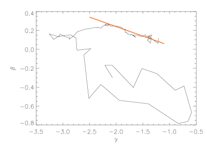
Figure 9: Velocity anisotropy $\beta$ as a function of the radial derivative of the density profile $\gamma$. The red solid line corresponds to equation (47) (Hansen & Stadel, 2003).

Figure 10: Logarithmic derivative of the radial velocity dispersion $\kappa$, as defined by equation 49.

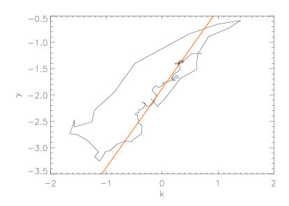
Figure 11: Derivative of the radial velocity dispersion $\kappa$ as a function of the logarithmic slope of the density profile $\gamma$. The red solid line corresponds to the equation (50) (Taylor & Navarro, 2001; Ludlow et al., 2011).

References

- Ascasibar & Gottlöber (2008) Ascasibar Y., Gottlöber S., 2008, MNRAS, 386, 2022
- Bertschinger (1985) Bertschinger E., 1985, ApJS, 58, 39
- Binney & Mamon (1982) Binney J., Mamon G. A., 1982, MNRAS, 200, 361
- Borgani et al. (2004) Borgani S. et al., 2004, MNRAS, 348, 1078
- Bryan & Norman (1998) Bryan G. L., Norman M. L., 1998, ApJ, 495, 80
- Cole & Lacey (1996) Cole S., Lacey C., 1996, MNRAS, 281, 716
- Cuesta et al. (2008) Cuesta A. J., Prada F., Klypin A., Moles M., 2008, MNRAS, 389, 385
- Cunha et al. (2009) Cunha C., Huterer D., Frieman J. A., 2009, Phys. Rev. D, 80, 63532
- Diaferio (1999) Diaferio A., 1999, MNRAS, 309, 610
- Ettori et al. (2002) Ettori S., Fabian A. C., Allen S. W., Johnstone R. M., 2002, MNRAS, 331, 635
- Fakhouri et al. (2010) Fakhouri O., Ma C.-P., Boylan-Kolchin M., 2010, MNRAS, 406, 2267
- Falco et al. (2013) Falco M., Hansen S., Wojtak R., Mamon G. A., 2013, MNRAS, 431, L6
- Girardi et al. (1998) Girardi M., Giuricin G., Mardirossian F., Mezzetti M., Boschin W., 1998, ApJ, 505, 74
- Gunn & Gott (1972) Gunn J. E., Gott, III J. R., 1972, ApJ, 176, 1
- Haiman et al. (2001) Haiman Z., Mohr J. J., Holder G. P., 2001, ApJ, 553, 545
- Hansen & Stadel (2003) Hansen S. H., Stadel J., 2003, ApJ, 595, L37
- Host & Hansen (2011) Host O., Hansen S. H., 2011, ApJ, 736, 52
- Karachentsev & Nasonova (2010) Karachentsev I. D., Nasonova O. G., 2010, MNRAS, 405, 1075
- Katgert et al. (2004) Katgert P., Biviano A., Mazure A., 2004, ApJ, 600, 657
- Kravtsov et al. (1998) Kravtsov A. V., Klypin A. A., Bullock J. S., Primack J. R., 1998, ApJ, 502, 48
- Łokas & Mamon (2003) Łokas E. L., Mamon G. A., 2003, MNRAS, 343, 401
- Łokas et al. (2006) Łokas E. L., Wojtak R., Gottlöber S., Mamon G. A., Prada F., 2006, MNRAS, 367, 1463
- Lombriser (2011) Lombriser L., 2011, Phys. Rev. D, 83, 63519
- Ludlow et al. (2011) Ludlow A. D., Navarro J. F., White S. D. M., Boylan-Kolchin M., Springel V., Jenkins A., Frenk C. S., 2011, MNRAS, 415, 3895
- Mahajan et al. (2011) Mahajan S., Mamon G. A., Raychaudhury S., 2011, MNRAS, 416, 2882
- Mamon & Boué (2010) Mamon G. A., Boué G., 2010, MNRAS, 401, 2433
- Mamon & Łokas (2005) Mamon G. A., Łokas E. L., 2005, MNRAS, 363, 705
- Mamon et al. (2004) Mamon G. A., Sanchis T., Salvador-Solé E., Solanes J. M., 2004, A&A, 414, 445
- Mamon et al. (2012) Mamon G. A., Tweed D., Thuan T. X., Cattaneo A., Papaderos P., Recchi S., Hensler G., 2012, Predicting the Frequencies of Young and of Tiny Galaxies., Springer-Verlag, Berlin, p. 39
- Mandelbaum et al. (2010) Mandelbaum R., Seljak U., Baldauf T., Smith R. E., 2010, MNRAS, 405, 2078
- Mei et al. (2007) Mei S. et al., 2007, ApJ, 655, 144
- Mohayaee & Tully (2005) Mohayaee R., Tully R. B., 2005, ApJ, 635, L113
- More et al. (2011) More S., Kravtsov A. V., Dalal N., Gottlöber S., 2011, ApJS, 195, 4
- Navarro et al. (1996) Navarro J. F., Frenk C. S., White S. D. M., 1996, ApJ, 462, 563
- Neistein & Dekel (2008) Neistein E., Dekel A., 2008, MNRAS, 383, 615
- Peebles (1993) Peebles P. J. E., 1993, Princeton Series in Physics: Principles of Physical Cosmology. Princeton Univ. Press, Princeton, NJ
- Power et al. (2012) Power C., Knebe A., Knollmann S. R., 2012, MNRAS, 419, 1576
- Rines & Diaferio (2006) Rines K., Diaferio A., 2006, AJ, 132, 1275
- Schmidt & Allen (2007) Schmidt R. W., Allen S. W., 2007, MNRAS, 379, 209
- Serra et al. (2011) Serra A. L., Diaferio A., Murante G., Borgani S., 2011, MNRAS, 412, 800
- Taylor & Navarro (2001) Taylor J. E., Navarro J. F., 2001, ApJ, 563, 483
- Voit (2005) Voit G. M., 2005, Rev. Mod. Phys., 77, 207
- Wechsler et al. (2002) Wechsler R. H., Bullock J. S., Primack J. R., Kravtsov A. V., Dekel A., 2002, ApJ, 568, 52
- Wojtak & Łokas (2010) Wojtak R., Łokas E. L., 2010, MNRAS, 408, 2442
- Wojtak et al. (2005) Wojtak R., Łokas E. L., Gottlöber S., Mamon G. A., 2005, MNRAS, 361, L1
- Wojtak et al. (2009) Wojtak R., Łokas E. L., Mamon G. A., Gottlöber S., 2009, MNRAS, 399, 812
- Wojtak et al. (2008) Wojtak R., Łokas E. L., Mamon G. A., Gottlöber S., Klypin A., Hoffman Y., 2008, MNRAS, 388, 815
- Zappacosta et al. (2006) Zappacosta L., Buote D. A., Gastaldello F., Humphrey P. J., Bullock J., Brighenti F., Mathews W., 2006, ApJ, 650, 777
- Zhao et al. (2003) Zhao D. H., Mo H. J., Jing Y. P., Börner G., 2003, MNRAS, 339, 12
- Zu & Weinberg (2013) Zu Y., Weinberg D. H., 2013, MNRAS, 431, 3319
- Zwicky (1933) Zwicky F., 1933, Helv. Phys. Acta, 6, 110