Thermophysical properties of hydrogen-helium mixtures: re-examination of the mixing rules via quantum molecular dynamics simulations

Abstract

Thermophysical properties of hydrogen, helium, and hydrogen-helium mixtures have been investigated in the warm dense matter regime at electron number densities ranging from $6.02\times 10^{29}\sim 2.41\times 10^{30}$/m³ and temperatures from 4000 to 20000 K via quantum molecular dynamics simulations. We focus on the dynamical properties such as the equation of states, diffusion coefficients, and viscosity. Mixing rules (density matching, pressure matching, and binary ionic mixing rules) have been validated by checking composite properties of pure species against that of the fully interacting mixture derived from QMD simulations. These mixing rules reproduce pressures within 10% accuracy, while it is 75 % and 50 % for the diffusion and viscosity, respectively. Binary ionic mixing rule moves the results into better agreement. Predictions from one component plasma model are also provided and discussed.

I Introduction

The study of the equation of state (EOS), transport properties, and mixing rules of hydrogen (H) and helium (He) under extreme condition of high pressure and temperature is not only of fundamental interest but also of essential practical applications for astrophysics Hubbard:1981 . For instance, giant planets such as Jupiter and Saturn require accurate EOS as the basic input into the respective interior models in order to solve hydrostatic equation and investigate the solubility of the rocky core Wilson:2012:a ; Wilson:2012:b . On the other side, the evolution of stars and the design of thermal protection system is assisted by high precision transport coefficients of H-He mixtures at high pressure Bruno:2010 . In addition, the viscosity and mutual diffusion coefficients are also important input properties for hydrodynamic simulations in modelling the stability of the hot spot-fuel interfaces and the degree of fuel contamination in inertial confinement fusion (ICF) Atzeni:2004 ; Lindl:1998 .

Since direct experimental access such as shock wave experiments is limited in the Mbar regime Knudson:2009 , the states deep in the interior of Jupiter ($\sim 45$ Mbar) and Saturn ($\sim 10$ Mbar) Lorenzen:2009 can not be duplicated in the laboratory. As a consequence, theoretical modelling provides most of the insight into the internal structure of Giant planets. The EOS of H-He mixtures have been treated by a linear mixing (LM) of the individual EOS via fluid perturbation theory Stevenson:1975 and Monte Carlo simulations Hubbard:1985 . Recently, several attempts have been made to calculate EOS of H-He mixtures by means of quantum molecular dynamic (QMD) simulations. Klepeis et al. Klepeis:1991 applied local density approximation of density functional theory (LDA-DFT) calculations for solid H-He mixtures, implying demixing for Jupiter and Saturn at 15000 K for a He fraction of $x=N_{He}/(N_{He}+N_{H})=0.07$. Vorberger et al. Vorberger:2007 , Lorenzen et al. Lorenzen:2009 , and Militzer Militzer:2013 performed QMD simulations by using generalized gradient expansion (GGA) instead of the LDA in order to evaluate the accuracy of the LM approximation and study the demixing of H-He at Mbar pressures. Pfaffenzeller et al. Pfaffenzeller:1995 introduced Car-Parrinello molecular dynamics (CPMD) simulations to calculate the excess Gibbs free energy of mixing at a lower temperature compared to that set in the work of Lorenzen et al. Lorenzen:2009 and Militzer Militzer:2013 .

Considering the transport properties, QMD Wang:2011 and orbital-free molecular dynamics (OFMD) Recoules:2009 simulations have been introduced to study hydrogen and its isotropic deuterium (D) and tritium (T). Self-diffusion coefficients in the pure H system and mutual diffusion for D-T mixtures were determined for temperatures $T=$1 to 10 eV and equivalent H mass densities 0.1 to 8.0 g/cm³ Collins:1994 ; Kwon:1994 ; Collins:1995 ; clerouin:1997 ; Kwon:1995 ; clerouin:2001 ; Kress:2010 . QMD and OFMD simulations of self-diffusion, mutual diffusion, and viscosity have recently been performed on heavier elements (Fe, Au, Be) Lambert:2006:a ; Lambert:2006:b ; Wang:2013 and on mixtures of Li and H Horner:2009 .

The present work selects H-He mixture as a representative system and examines some of the standard mixing rules with respect to the EOS and transport properties (viscosity, self and mutual diffusion coefficients) in the warm dense regime that covers standard extreme condition as reached in the interiors of Jupiter and Saturn. The thermophysical properties of the full mixture and the individual species have been derived from QMD simulations, where the electrons are quantum mechanically treated through finite-temperature (FT) DFT and ions move classically. In the next section, we present the formalism for QMD and for determining the static and transport properties. Then, EOS, viscosity, and diffusion coefficients for H-He mixtures are presented, and the QMD results are compared with the results from reduced models and QMD based linear mixing models. Finally, concluding remarks are given.

II FORMALISM

In this section, a brief description of the fundamental formalism employed to investigate H-He mixtures is introduced. The basic quantum mechanical density functional theory forms the basis of our simulations. The implementation of schemes in determining diffusion and viscosity is discussed. Mixing rules that combine pure species quantities to form composite properties is also presented.

II.1 Quantum molecular dynamics

QMD simulations have been performed for H-He mixtures by using Vienna ab initio Simulation Package (VASP) Kresse1993 ; Kresse1996 . In these simulations, the electrons are treated fully quantum mechanically by employing a plane-wave FT-DFT description, where the electronic states follow the Fermi-Dirac distribution. The ions move classically according to the forces from the electron density and the ion-ion repulsion. Simulations have been performed in the NVT (canonical) ensemble where the number of particles $N$ and the volume are fixed. The system was assumed to be in local thermodynamic equilibrium with the electron and ion temperatures being equal ($T_{e}=T_{i}$). In these calculations, the electronic temperature has been kept constant according to Fermi-Dirac distribution, and ion temperature is controlled by Nośe thermostat Hunenberger2005 .

At each step during MD simulations, a set of electronic state functions [$\Psi_{i,k}(r,t)$] for each k-point are determined within Kohn-Sham construction by

$$H_{KS}\Psi_{i,k}(r,t)=\epsilon_{i,k}\Psi_{i,k}(r,t),$$ (1)

with

$$H_{KS}=-\frac{1}{2}\nabla^{2}+V_{ext}+\int\frac{n(r^{\prime})}{|r-r^{\prime}|}dr^{\prime}+v_{xc}(r),$$ (2)

in which the four terms respectively represent the kinetic contribution, the electron-ion interaction, the Hartree contribution and the exchange-correlation term. The electronic density is obtained by

$$n(r)=\sum_{i,k}f_{i,k}|\Psi_{i,k}(r,t)|^{2}.$$ (3)

Then by applying the velocity Verlet algorithm, based on the force from interactions between ions and electrons, a new set of positions and velocities are obtained for ions.

All simulations are performed with 256 atoms and 128 atoms for pure species of H and He, and as for the case of the H-He mixture, a total number of 245 atoms (234 H atoms and 11 He atoms) for a mixing ratio $x=\frac{2N_{He}}{N_{H}+2N_{He}}=8.59\%$ (corresponding to the H-He immiscibility region determined in the work of Morales et al. Morales2009 ) has been adopted, where a cubic cell of length $L$ (volume $V=L^{3}$) is periodically repeated. The simulated densities range from 1.0 to 4.0 g/cm³ for pure H system. As for pure He and H-He mixture, the size of the supercell is chosen to be the same as that for pure H to secure a constant electron number density (in the range $6.02\times 10^{29}\sim 2.41\times 10^{30}$/m³). The temperature from 4000 K to 20000 K has been selected to highlight the conditions in the interiors of Jupiter and Saturn. The convergence of the thermodynamic quantities plays an important role in the accuracy of QMD simulations. In the present work, a plane-wave cutoff energy of 1200 eV is employed in all simulations so that the pressure is converged within 2%. We have also checked out the convergence with respect to a systematic enlargement of the k-point set in the representation of the Brillouin zone. In the molecular dynamic simulations, only the $\Gamma$ point of Brillouin zone is included. The dynamic simulation is lasted 20000 steps with time steps of 0.2 $\sim$ 0.7 fs according to different densities and temperatures. For each pressure and temperature, the system is equilibrated within 0.5 $\sim$ 1 ps. The EOS data are obtained by averaging over the final 1 $\sim$ 3 ps molecular dynamic simulations.

II.2 Transport properties

The self-diffusion coefficient $D$ can either be calculated from the trajectory by the mean-square displacement

$$D=\frac{1}{6t}\langle|R_{i}(t)-R_{i}(0)|^{2}\rangle,$$ (4)

or by the velocity autocorrelation function

$$D=\frac{1}{3}\int_{0}^{\infty}\langle V_{i}(t)\cdot V_{i}(0)\rangle dt,$$ (5)

where $R_{i}$ is the position and $V_{i}$ is the velocity of the $i$th nucleus. Only in the long-time limit, these two formulas of $D$ are formally equivalent. Sufficient lengths of the trajectories have been generated to secure contributions from the velocity autocorrelation function to the integral is zero, and the mean mean-square displacement away from the origin consistently fits to a straight line. The diffusion coefficient obtained from these two approaches lie within 1 % accuracy of each other. Here, we report the results from velocity autocorrelation function.

We have also computed the mutual-diffusion coefficient

$$D_{\alpha\beta}=\lim_{t\rightarrow\infty}\overline{D_{\alpha\beta}}(t)$$ (6)

from the autocorrelation function

$$\overline{D_{\alpha\beta}}(t)=\frac{Q}{3Nx_{\alpha}x_{\beta}}\int_{0}^{t}\langle A(0)A(t^{\prime})\rangle dt^{\prime}$$ (7)

with

$$A(t)=x_{\beta}\sum_{i=1}^{N_{\alpha}}V_{i}(t)-x_{\alpha}\sum_{j=1}^{N_{\beta}}V_{j}(t),$$ (8)

where the concentration and particle number of species $\alpha$ are denoted by $x_{\alpha}$ and $N_{\alpha}$, respectively, and the total number of particles in the simulation box $N=\sum_{\alpha}N_{\alpha}$. The quantity $Q$ is the thermodynamic factor related to the second derivation of the Gibbs free energy with respect to concentrations Hansen1986 . In the present simulations, $Q$ value has been adopted equal to unity since studies with Leonard-Jones and other model potentials have shown that for dissimilar constituents the $Q$-factor departs from unity by about 10% Schoen1984 .

The viscosity

$$\eta=\lim_{t\rightarrow\infty}\bar{\eta}(t),$$ (9)

has been computed from the autocorrelation function of the off-diagonal component of the stress tensor Allen1987

$$\bar{\eta}(t)=\frac{V}{k_{B}T}\int_{0}^{t}\langle P_{12}(0)P_{12}(t^{\prime})\rangle dt^{\prime}.$$ (10)

The results are averaged from the five independent off-diagonal components of the stress tensor $P_{xy}$, $P_{yz}$, $P_{zx}$, $(P_{xx}-P_{yy})/2$, and $(P_{yy}-P_{zz})/2$.

Different from the self-diffusion coefficient, which involves single-particle correlations and attains significant statistical improvement from averaging over the particles, the viscosity depends on the entire system and thus needs very long trajectories so as to gain statistical accuracy. To shorten the length of the trajectory, we use empirical fits Kress2011 to the integrals of the autocorrelation functions. Thus, extrapolation of the fits to $t\rightarrow\infty$ can more effectively determine the basic dynamical properties. Both of the $D$ and $\bar{\eta}$ have been fit to the functional in the form of $A[1-\exp(-t/\tau)]$, where $A$ and $\tau$ are free parameters. Reasonable approximation to the viscosity can be produced from the finite time fitting procedure, which also serves to damp the long-time fluctuations.

The fractional statistical error in calculating a correlation function $C$ for molecular-dynamics trajectories Zwanzig1969 can be given by

$$\frac{\vartriangle C}{C}=\sqrt{\frac{2\tau}{T_{traj}}},$$ (11)

where $\tau$ is the correlation time of the function, and $T_{traj}$ is the length of the trajectory. In the present work, we generally fitted over a time interval of [0, $4\tau-5\tau$].

II.3 Mixing rules

Here, we examine two representative mixing rules. The first, termed density-matching rule (MRd) with the inspiration of a two-species ideal gas. The second, termed pressure-matching rule (MRp), which follows from two interacting immiscible fluids.

In the MRd, the volume of the individual species is set equal to that of the mixture ($V_{H}=V_{He}=V_{H-He}$), and QMD simulations are performed for H at a density of $N_{H}/V_{H-He}$ and He at $N_{He}/V_{H-He}$ at a temperature $T$. Then, pressure predicted by MRd is determined by simply adding the individual pressures from the pure species H and He simulations. Other transport coefficients, such as mutual diffusion and viscosity, follow the same prescription and are summarized as

$$\begin{split}V_{H-He}=&V_{H}=V_{He},\\ P_{H-He}^{d}=&P_{H}+P_{He},\\ D_{H-He}^{d}=&D_{H}+D_{He},\\ \eta_{H-He}^{d}=&\eta_{H}+\eta_{He}.\end{split}$$ (12)

The superscript is used to denote values predicted from MRd. The derived pressure based on density mixing rule generally follows from the ideal noninteracting H and He gas in a volume $V_{H-He}$.

The MRp has a more complicated construction compared to MRd. MRp can be characterized as the following prescription:

$$\begin{split}V_{H-He}=&V_{H}+V_{He},\\ P_{H-He}^{p}=&P_{H}=P_{He},\\ D_{H-He}^{p}=&\nu_{H}D_{H}+\nu_{He}D_{He},\\ \eta_{H-He}^{p}=&\nu_{H}\eta_{H}+\nu_{He}\eta_{He}.\end{split}$$ (13)

In this case, we have performed a series of QMD simulations on the individual species H and He, where the volumes change under a constraint $(V_{H-He}=V_{H}+V_{He})$ until the individual pressures equal to each other $(P_{H}=P_{He})$. The total pressure becomes the predicted value. Here, we use the excess or electronic pressure $P_{e}$ to evaluate this MRp mixing rule. Composite properties such as mutual diffusion and viscosity are evaluated by combining the individual species results via volume fractions $(\nu_{\alpha}=V_{\alpha}/V_{H-He})$.

Finally, we also derive properties of the mixture from a slightly more complex mixing rule Bastea2005 , as so-called binary ionic mixture (BIM):

$$\sum_{i}\nu_{i}\frac{\gamma_{i}-\gamma_{m}}{\gamma_{i}+\frac{3}{2}\gamma_{m}}=0$$ (14)

with $\gamma$ the predicted mutual-diffusion coefficient or the viscosity. The subscript $m$ denotes the mixture and $i$ the pure species.

III Results And Discussion

In this section, the wealth of information derived from QMD calculations are mainly presented through figures, and the general trends of the EOS as well as transport coefficients are concentrated in the text. It is, therefore, interesting to explore not only to get insight into the interior physical properties of giant gas planets but also to examine a series of mixing rules for hydrogen and helium. Additionally, one can consider the influence of helium on the EOS and transport coefficients of mixing.

III.1 The equation of state

High precision EOS data of hydrogen and helium are essential for understanding the evolution of Jupiter and target implosion in ICF. Experimentally, The EOS of hydrogen and helium in the fluid regime have been studied through gas gun Nellis2006 , chemical explosive Boriskov2005 , magnetic driven plate flyer Knudson2004 , and high power laser Collins1998 ; Boehly2004 ; Hicks2009 . Since these experiments were limited by the conservation of mass, momentum, and energy, the explored density of warm dense matter were limited within $5\sim 6$ times of the initial density. Recently, a new technique combined diamond anvil cell (DAC) and high intensity laser pulse has successfully been proved to provide visible ways to generate shock Huguniot data of hydrogen over a significantly broader density-temperature regime than previous experiments Loubeyre2012 . However, the density therein was still restricted within 1 g/cm³.

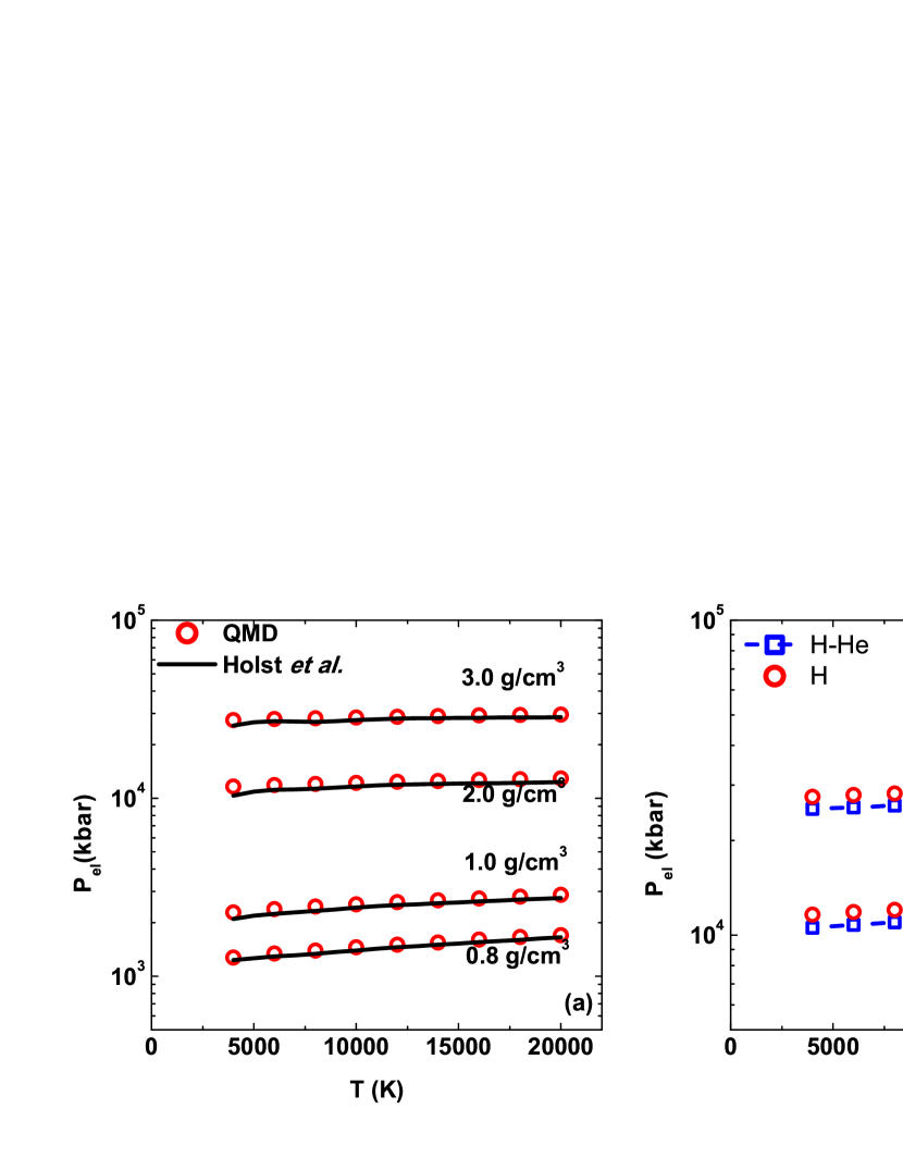
Figure 1: (Color online) The present simulated QMD EOS have been shown as a function of temperature (with error bar smaller than the symbolic size). (a) Comparison with the results of Holst et al. Holst2008 for hydrogen; (b) The variation in EOS after considering the mixing of helium.

In our simulations, wide range EOS for H, He, and H-He mixtures have been determined according to QMD method. The EOS can be divided into two parts That is, contributions from the noninteracting motion of ions ($P_{i}$) and the electronic term ($P_{el}$),

$$P_{total}=P_{i}+P_{el},$$ (15)

where $P_{el}$ is calculated directly through DFT. In Fig. 1 (a), we have compared our results of $P_{el}$ with that of Holst et al. Holst2008 , where the electronic pressure is expressed as a smooth function in terms of density and temperature, and the results agree with each other with a very slight difference (accuracy within 5%). In the simulated density and temperature regime, we do not find any signs indicating a liquid-liquid phase transition ($\frac{\partial P}{\partial T}|_{V}<0$) or plasma phase transition ($\frac{\partial P}{\partial V}|_{T}>0$), which are characterized by molecular dissociation and ionization of electrons, respectively. With considering the mixing of He into H, the electronic pressure is effectively reduced, as has been shown in Fig. 1 (b).

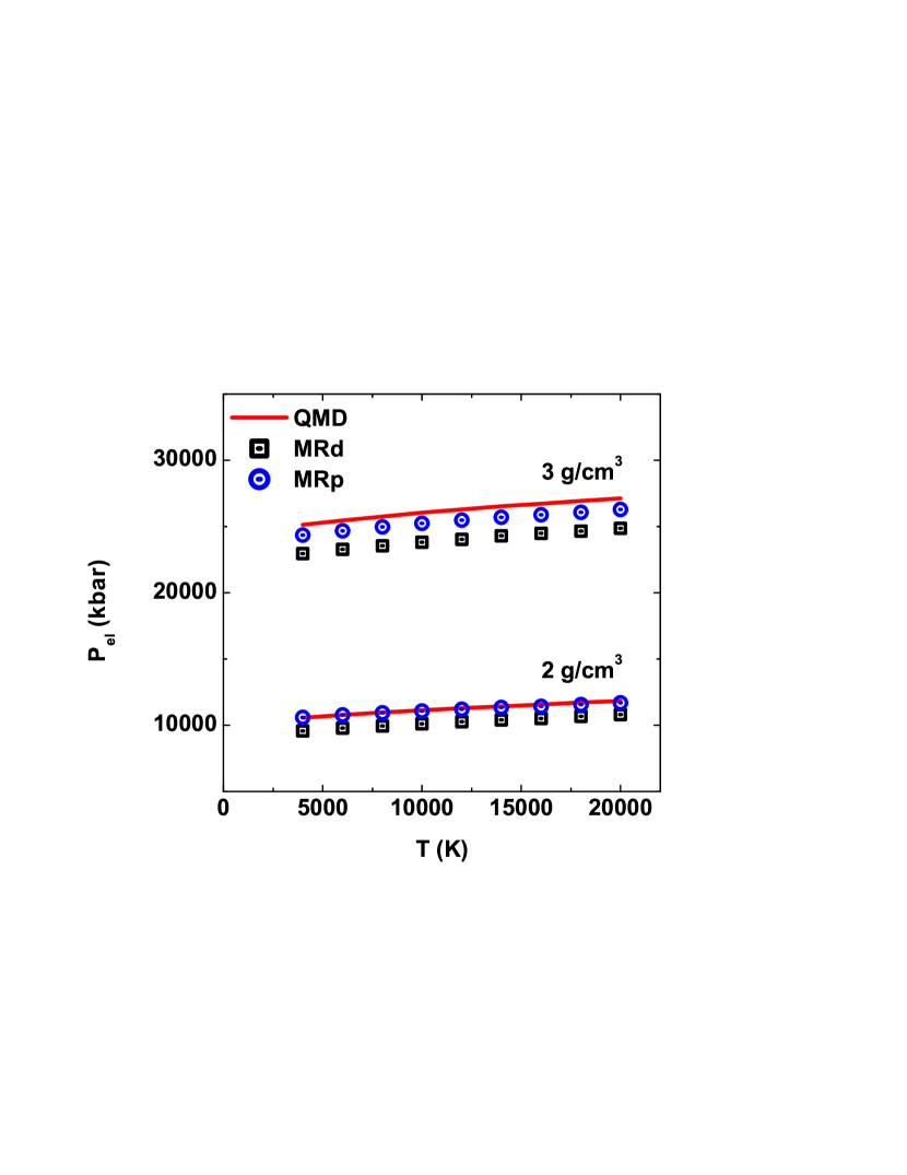
Figure 2: (Color online) Comparison of electronic pressure between direct QMD simulation results and those from mixing rules (error bar being smaller than symbol size). QMD results are denoted by red solid lines, while the MRd and MRp data are presented by open squares and open circles, respectively.

MRd accounts for contribution from noninteracting H and He subsystems in the volume of the mixtures. In MRd, the pressure contributed from noninteracting ions is the same as that of the mixture, but the electronic pressure is much lower due to the low electronic density in the pure species simulations. It is indicated that the electronic pressure is underestimated by MRd model at about 8% $\sim$ 9% (see Fig. 2). For MRp model, we have firstly performed a series of pure species simulations at a wider density (temperature) regime compared to H-He mixtures. Then, the simulated EOS data are fitted into smooth functions in terms of density and temperature. Under the constraint of $V_{H-He}=V_{H}+V_{He}$, we have predicted the electronic pressures $P_{H-He}=P_{H}=P_{He}$ according to MRp model by solving pure species EOS function at certain densities and temperatures, as shown in Fig. 2. It is indicated that the MRp model agrees better with direct QMD simulations (accuracy within 3%), the difference mainly come from the ionic interactions between H and He species after mixing.

III.2 Diffusion and viscosity

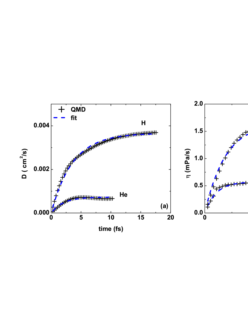
Figure 3: (Color online) Transport properties are shown for H and He at 12000 K with densities of 2 g/cm³ and 8 g/cm³, respectively. (a) Self-diffusion coefficient; (b) Viscosity. The direct QMD simulated results are presented by black crosses, while the fitted results are denoted by blue dashed lines.

QMD simulations have been performed within the framework of FT-DFT to benchmark the dynamic properties of H, He, and H-He mixture in the WDM regime. Illustrations for the self-diffusion coefficients and viscosity (for H and He at densities of 2.0 g/cm³ and 8.0 g/cm³, respectively) at a temperature 12000 K, as well as their fits are shown in Fig. 3. The trajectory of the present simulations lasts 4.0 $\sim$ 14.0 ps, and correlation times between 1.0 and 15.0 fs. As a consequence, the computational error for the viscosity lies within 10%. After accounting for the fitting error and extrapolation to infinite time, a total uncertainty of $\sim$ 20% can be estimated. The uncertainty in the self-diffusion coefficients is smaller than 1%, due to the additional $\frac{1}{\sqrt{N}}$ advantage given by particle average.

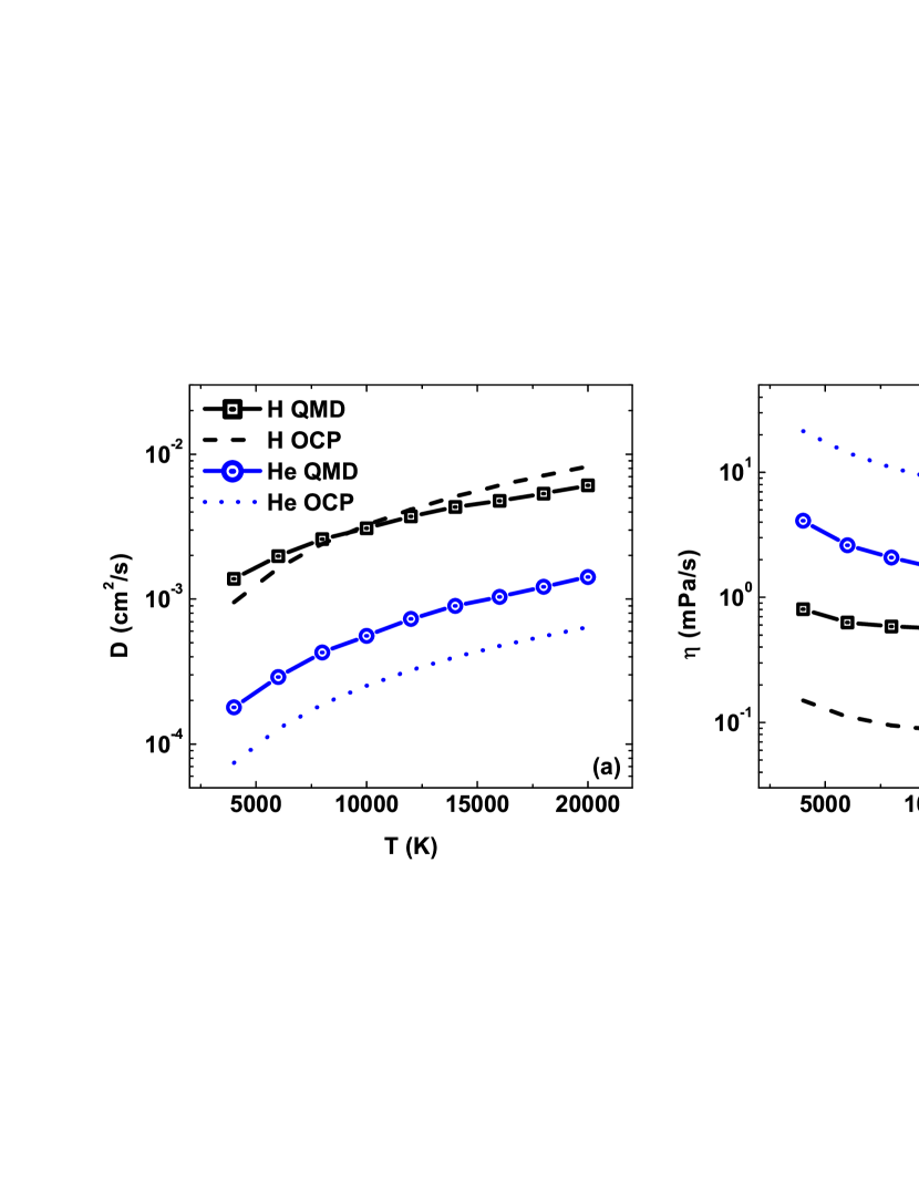
Figure 4: (Color online) Comparison between QMD simulations and OCP model (error bars are smaller than symbol size). (a) Self-diffusion coefficient; (b) Viscosity. The sampled density for hydrogen is 2 g/cm³. For helium, the density is 8 g/cm³. The electron number density for pure species (H and He) is $1.204\times 10^{30}$/m³.

Dynamic properties of WDM are generally governed by two dimensionless quantities, namely, ionic coupling ($\Gamma$) and electronic degenerate ($\theta$) parameter. The former one is defined by the ratio of the potential to kinetic energy $\Gamma=\frac{(Ze)^{2}}{ak_{B}T}$, with $Z$ the ionic charge, and $a=(3/4\pi n_{i})^{1/3}$ the ion-sphere radius ($n_{i}$ is the number density). The latter one $\theta=T/T_{F}$, where $T_{F}$ is Fermi temperature. It has been reported that dynamic properties such as diffusion coefficients and viscosity can be represented purely in terms of ionic coupling parameter $\Gamma$ according to molecular dynamics or Monte Carlo simulations based on one component plasma (OCP) model Bastea2005 ; Lambert2007 ; Bernu1978 ; Donko1998 ; Daligault2006 ; Hansen1975 , where ions move classically in a neutralizing background of electrons. For instance, Hansen et al. Hansen1975 introduced a memory function to analyze the velocity autocorrelation function, and obtain the diffusion coefficient in terms of $D=2.95\Gamma^{-1.34}\omega_{p}a^{2}$ with the plasma frequency $\omega_{p}=(4\pi n_{i}/M)^{1/2}Ze$. Based on classical molecular dynamic simulations, Bastea Bastea2005 has fitted the viscosity into the following form

$$\eta=(A\Gamma^{-2}+B\Gamma^{-s}+C\Gamma)n_{i}M\omega_{p}a^{2},$$ (16)

with $s=0.878$, $A=0.482$, $B=0.629$, and $C=0.00188$.

Since OCP model is restricted to a fully ionized plasma, we use $Z$=1.0 (or 2.0) for hydrogen (or helium) to compute the self-diffusion coefficient and viscosity. In Fig. 4 (a), we show comparison between QMD and OCP model Hansen1975 for hydrogen and helium at densities of 2 g/cm³ and 8 g/cm³. The general tendency for the self-diffusion coefficient with respect to temperature is similar for QMD and OCP model, however, the difference up to $\sim$60 % is observed between the two results. For the viscosity [Fig. 4 (b)], OCP Bastea2005 predicts smaller (larger) values for hydrogen (helium) compared to QMD simulations. The viscosity is governed by interactions between particles and ionic motions, contribution from the former one decrease with the increase of temperature, while, it increases for the latter one. As a consequence, the viscosity may have local minimum along temperature. For hydrogen, the local minimum locates around 10000 K and 14000 K indicated by QMD and OCP model, respectively. While in the case of helium, we do not observe any signs for the local minimum in the simulated regime.

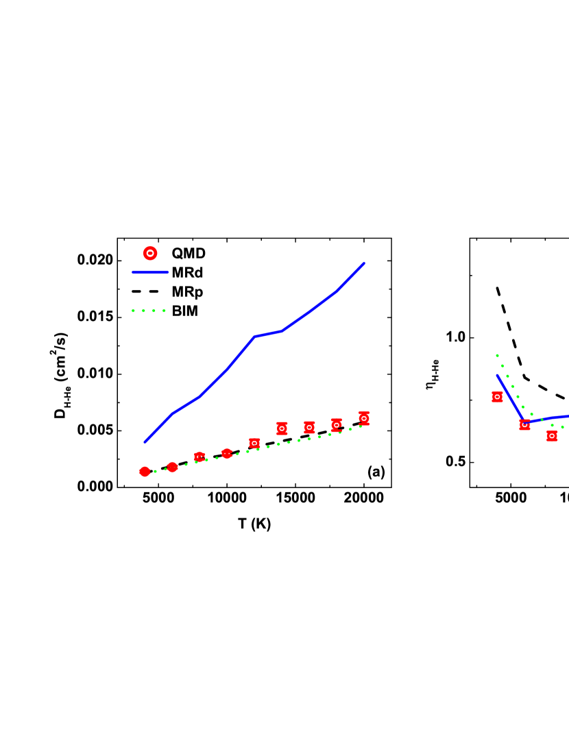
Figure 5: (Color online) Comparison between QMD simulations and mixing rules. (a) Mutual-diffusion coefficient; (b) Viscosity. The sampled mixture has a electron number density of $1.204\times 10^{30}$/m³ and temperature from 4000 $\sim$ 20000 K.

In Fig. 5, we have shown the mutual diffusion coefficient $D_{H-He}$ and viscosity $\eta_{H-He}$ for H-He mixture with an electron number density of $1.204\times 10^{30}$/m³, and results from mixing models are also provided. The transport coefficients predicted by MRd can be directly evaluated through Eq. (12). For MRp model, we have firstly fitted the self-diffusion coefficients and viscosity in terms of density and temperature, after determining the volume for each species under the constraint of $P_{H}=P_{He}$, the transport coefficients are then obtained. In BIM model, we have used $\nu_{H}=91.41\%$ and $\nu_{He}=8.59\%$, then, the transport coefficients are determined by Eq. (14). Here we would like to stress that in some mixture studies based on average atom models More1985 , the properties of pure species are derived from perturbed-atom models, where boundary conditions are introduced from the surrounding medium by treating a single atom within a cell. In the present work, the dynamic properties of different mixing rules originate from QMD calculations of the individual species. Despite divorced of the H-He interactions, the pure species calculations still contain complex intra-atomic interactions based on large samples of atoms.

The mutual diffusion coefficient of H-He mixture shows a linear increase with respect of temperature, as indicated in Fig. 5(a). The data from MRp and BIM models have a better agreement with QMD simulations compared with that of the MRd model, where ion densities are reduced and results in a larger diffusion coefficient. The viscosity of H-He mixture has a more complex behavior than pure species under extreme condition. As shown in Fig. 5 (b), MRd is valid at low temperature, while MRp works at higher temperature. BIM rule moves the results into better agreement with the H-He mixture, leaving within 30% or better for the simulated conditions.

IV Conclusion

In summary, we have performed systematic QMD simulations of H, He, and H-He mixture in the warm dense regime for electron number density ranging from $6.02\times 10^{29}\sim 2.41\times 10^{30}$/m³ and for temperatures from 4000 to 20000 K. The present study concentrated on thermophysical properties such as the EOS, diffusion coefficient, and viscosity, which are of crucial interest in astrophysics and ICF. Various mixing rules have been introduced to predict dynamical properties from QMD simulations of the pure species and compare with direct calculations on the fully interacting mixture. We have shown that MRd and MRp rules produce pressures within about 10 % of the H-He mixture, however, the mutual diffusion coefficients are as different as 75 % and it is 50 % for the viscosity. BIM rule generally gives better agreement with the mixture results. We have also compared our QMD results with OCP model for the pure species.

- (1) W. B. Hubbard, Science 214, 145 (1981).
- (2) H. F. Wilson and B. Militzer, Astrophys. J. 745, 54 (2012).
- (3) H. F. Wilson and B. Militzer, Phys. Rev. Lett. 108, 111101 (2012).
- (4) D. Bruno, C. Catalfamo, M. Capitelli, G. Colonna, O. De Pascale, P. Diomede, C. Gorse, A. Laricchiuta, S. Longo, D. Giordano, and F. Pirani, Phys. Plasmas 17, 112315 (2010).
- (5) S. Atzeni and J. Meyer-ter-Vehn, The Physics of Inertial Fusion: Beam Plasma Interaction, Hydrodynamics, Hot Dense Matter, International Series of Monographs on Physics (Clarendon Press, Oxford, 2004).
- (6) J. D. Lindl, Inertial Confinement Fusion: The Quest for Ignition and Energy Gain Using Indirect Drive, (Springer-Verlag, New York, 1998).
- (7) M. D. Knudson and M. P. Desjarlais, Phys. Rev. Lett. 103, 225501 (2009).
- (8) W. Lorenzen, B. Holst, and R. Redmer, Phys. Rev. Lett. 102, 115701 (2009).
- (9) D. J. Stevenson, Phys. Rev. B 12, 3999 (1975).
- (10) W. B. Hubbard and H. E. DeWitt, Astrophys. J. 290, 388 (1985).
- (11) J. E. Klepeis, K. J. Schafer, T. W. Barbee III, and M. Ross, Science 254, 986 (1991).
- (12) J. Vorberger, I. Tamblyn, B. Militzer, and S. A. Bonev, Phys. Rev. B 75, 024206 (2007).
- (13) B. Militzer, Phys. Rev. B 87, 014202 (2013).
- (14) O. Pfaffenzeller, D. Hohl, and P. Ballone, Phys. Rev. Lett. 74, 2599 (1995).
- (15) C. Wang, X.-T. He, and P. Zhang, Phys. Rev. Lett. 106, 145002 (2011).
- (16) V. Recoules, F. Lambert, A. Decoster, B. Canaud, and J. Clérouin, Phys. Rev. Lett. 102, 075002 (2009).
- (17) L. A. Collins, J. D. Kress, D. L. Lynch, and N. Troullier, J. Quant. Spectrosc. Radiat. Transf. 51, 65 (1994).
- (18) I. Kwon, J. D. Kress, and L. A. Collins, Phys. Rev. B 50, 9118 (1994).
- (19) L. Collins, I. Kwon, J. Kress, N. Troullier, and D. Lynch, Phys. Rev. E 52, 6202 (1995).
- (20) J. Clérouin and S. Bernard, Phys. Rev. E 56, 3534 (1997).
- (21) I. Kwon, L. Collins, J. Kress, and N. Troullier, EPL 29, 537 (1995).
- (22) J. Clérouin and J.-F. Dufrêche, Phys. Rev. E 64, 066406 (2001).
- (23) J. D. Kress, J. S. Cohen, D. A. Horner, F. Lambert, and L. A. Collins, Phys. Rev. E 82, 036404 (2010).
- (24) F. Lambert, J. Cléouin, and S. Mazevet, EPL 75, 681 (2006).
- (25) F. Lambert, J. Cléouin, and G. Zérah, Phys. Rev. E 73, 016403 (2006).
- (26) C. Wang, Y. Long, X.-T. He, and P. Zhang, Phys. Rev. E 87, 043105 (2013).
- (27) D. A. Horner, F. Lambert, J. D. Kress, and L. A. Collins, Phys. Rev. B 80, 024305 (2009).
- (28) G. Kresse and J. Hafner, Phys. Rev. B 47, R558 (1993).
- (29) G. Kresse and J. Furthmüller, Phys. Rev. B 54, 11169 (1996).
- (30) P. H. Hünenberger, Adv. Polym. Sci. 173, 105 (2005); D. J. Evans and B. L. Holian, J. Chem. Phys. 83, 4069 (1985).
- (31) M. A. Morales, C. Pierleoni, E. Schwegler, and D. M. Ceperley, Proc. Natl. Acad. Sci. U.S.A. 106, 1324 (2009).
- (32) J. P. Hansen and I. R. McDonald, The Theory of Simple Liquids, 2nd ed. (Academic Press, New York, 1986), Chap. 8.
- (33) M. Schoen and C. Hoheisel, Mol.Phys. 52, 33 (1984); 52, 1029 (1984).
- (34) M. P. Allen and D. J. Tildesley, Computer Simulation of Liquids (Oxford University Press, New York, 1987).
- (35) J. D. Kress, James S. Cohen, D. P. Kilcrease, D. A. Horner, and L. A. Collins, Phys. Rev. E 83, 026404 (2011).
- (36) R. Zwanzig and N. K. Ailawadi, Phys. Rev. 182, 280 (1969).
- (37) S. Bastea, Phys. Rev. E 71, 056405 (2005).
- (38) W. J. Nellis, Rep. Prog. Phys. 69, 1479 (2006).
- (39) G. V. Boriskov, A. I. Bykov, R. Ilkaev, V. D. Selemir, G. V. Simakov, R. F. Trunin, V. D. Urlin, A. N. Shuikin, and W. J. Nellis, Phys. Rev. B 71, 092104 (2005).
- (40) M. D. Knudson, D. L. Hanson, J. E. Bailey, C. A. Hall, J. R. Asay, and C. Deeney, Phys. Rev. B 69, 144209 (2004).
- (41) G. W. Collins, L. B. Da Silva, P. Celliers, D. M. Gold, M. E. Foord, R. J. Wallace, A. Ng, S. V. Weber, K. S. Budil, and R. Cauble, Science 281, 1178 (1998).
- (42) T. R. Boehly, D. G. Hicks, P. M. Celliers, T. J. B. Collins, R. Earley, J. H. Eggert, D. Jacobs-Perkins, S. J. Moon, E. Vianello, D. D. Meyerhofer, and G. W. Collins, Phys. Plasmas 11, L49 (2004).
- (43) D. G. Hicks, T. R. Boehly, P. M. Celliers, J. H. Eggert, S. J. Moon, D. D. Meyerhofer, and G. W. Collins, Phys. Rev. B 79, 014112 (2009).
- (44) P. Loubeyre, S. Btygoo, J. Eggert, P. M. Celliers, D. K. Spaulding, J. R. Rygg, T. R. Boehly, G. W. Collins, and R. Jeanloz, Phys. Rev. B 86, 144115 (2012).
- (45) B. Holst, R. Redmer, and M. P. Desjarlais, Phys. Rev. B 77, 184201 (2008).
- (46) F. Lambert, Ph.D. thesis, Université Paris XI. Commissariatà l’ Énergie Atomique, 2007.
- (47) B. Bernu and P. Vieillefosse, Phys. Rev. A 18, 2345 (1978).
- (48) Z. Donkó, B. Nyíri, L. Szalai, and S. Holló, Phys. Rev. Lett. 81, 1622 (1998); Z. Donkó and B. Nyíri, Phys. Plasmas 7, 45 (2000).
- (49) J. Daligault,Phys. Rev. Lett. 96, 065003 (2006); 103, 029901(E) (2009).
- (50) J. P. Hansen, I. R. McDonald, and E. L. Pollock, Phys. Rev. A 11, 1025 (1975).
- (51) R. M. More, Adv. At. Mol. Phys. 21, 305 (1985).