Thèse de doctorat de
l’Ecole Normale Supérieure
Spécialité : Physique théorique
Présentée par
Benjamin ASSEL
pour obtenir le grade de
Docteur de l’Ecole Normale Supérieure

Sujet : Dualité Holographique pour Théories Superconformes en trois dimensions
Soutenance le 5 juillet 2013, devant le jury composé de

Henning Samtleben Rapporteur Amihay Hanany Rapporteur Michela Petrini Presidente Dario Martelli Examinateur Jan Troost Examinateur Costas Bachas Directeur de thèse

Thèse délivrée par l’Ecole Normale Supérieure, 45 rue d’Ulm, 75005 Paris FRANCE,
suite à des recherches effectuées au LPT-ENS, 24 rue Lhomond, 75005 Paris FRANCE,
dans le cadre de l’Ecole Doctorale de Physique de la Région Parisienne ED107.

Résumé

L’objet principal de la thèse consiste à exhiber et étudier une large classe de nouveaux exemples de correspondances holographiques de type AdS/CFT entre des théories de jauge super-conformes en trois dimensions avec $\mathcal{N}=4$ supersymétrie et la théorie des cordes de type IIB sur un espace $AdS_{4}\times K_{6}$ (produit de AdS à quatre dimension et d’un espace compact à six dimensions). Les théories de jauge superconformes en question sont obtenues comme points fixes infrarouges de théories de type Yang-Mills “quivers” (càd avec des produits de groupe unitaires comme groupe de jauge et un certain contenu en matière). Dans cette limite infrarouge le couplage de Yang-Mills est renormalisé et diverge ce qui rend ces théories inaccessibles à tout calcul perturbatif, d’où l’intérêt d’en avoir une description holographique.
Une large partie du manuscrit de thèse est consacrée à la présentation des solutions de supergravité et à l’établissement du dictionnaire avec les théories super-conformes. Les cas des quivers linéaires et circulaires sont traités, ainsi que les solutions de “domain wall”, qui correspondent à des théories Super-Yang-Mills à quatre dimensions couplées à un “défaut” à trois dimensions.
Plusieurs vérifications des correspondances sont données, notamment par le calcul de l’énergie libre qui est calculée du côté théorie de jauge, en utilisant certains résultats issus des techniques de localisation d’intégrales de chemin, et qui est comparée avec succès à l’action de supergravité.

Mots clés : Correspondance AdS/CFT, supergravité, supersymétrie, théorie des cordes, D-branes, dualités, énergie libre, modèles de matrice.

Holographic Duality for three-dimensional Super-conformal Field Theories

Abstract

We present a large class of new holographic dualities relating three-dimensional $\mathcal{N}=4$ super-conformal field theories and type IIB string theory on supergravity backgrounds, which have $AdS_{4}\times K_{6}$ metric. The superconformal theories arise as infrared fixed points of Yang-Mills quiver gauge theories (the gauge group is a product of unitary groups and the matter content is made of fundamental and bifundamental matter). In the infrared limit the Yang-Mills coupling diverges, so that the theories are strongly coupled and hence inaccessible to perturbative computations. This is a motivation for finding their dual holographic description.
The main part of the manuscript is devoted to the exposition of the supergravity solutions and to establishing the holographic dictionary. The cases of linear and circular quivers is covered entirely, as well as the domain wall solutions that are dual to 4d Super-Yang-Mills theory coupled to a half-BPS 3-dimensional defect field theory.
Several checks of the correspondences are given. Particularly we compute the free energy of the gauge theories, using the techniques of localization of path integral, and compare it successfully with the supergravity action.

Key words : AdS/CFT correspondence, supergravity, supersymmetry, string theory, D-branes, free energy, matrix models.

Contents

1. Acknowledgments
2. Presentation
   1. Résumé (français)
3. I Elements of AdS/CFT correspondence
   1. I.1 Low-energy descriptions of D3-branes
   2. I.2 Elements of correspondence
   3. I.3 Holographic renormalization of the gravity action
4. II 3d $\mathcal{N}=4$ quivers and brane realizations
   1. II.1 $\mathcal{N}=4$ supersymmetric gauge theories in 3 dimensions
      1. II.1.1 $\mathcal{N}=4$ supersymmetry in 3 dimensions and Lagrangian
      2. II.1.2 Mirror symmetry
      3. II.1.3 Matrix models
   2. II.2 Linear and circular quivers
   3. II.3 Brane Realization
   4. II.4 Defect SCFTs
   5. II.5 Partition function of deformed linear quivers
5. III Supergravity solutions and the correspondence
   1. III.1 History of the type IIB supergravity solution with $OSp(4|4)$ symmetry
   2. III.2 Solutions of IIB supergravity : the case of the strip
      1. III.2.1 Local solutions
      2. III.2.2 Admissible singularities
      3. III.2.3 Linear-quiver geometries and AdS/CFT dictionary
      4. III.2.4 Defect SCFT solutions
   3. III.3 Circular quiver geometries : from strip to annulus
      1. III.3.1 Solutions on the annulus
      2. III.3.2 Calculation of D3-brane charges
      3. III.3.3 Correspondence and 5-brane moves
   4. III.4 Limiting geometries
      1. III.4.1 Wormbrane limits
      2. III.4.2 Large-$L$ limit and M2 branes
      3. III.4.3 Supergravity regimes of parameters
6. IV Testing the correspondence : free energy calculations
   1. IV.1 CFT Analysis
      1. IV.1.1 The $S^{3}$ Partition Function
      2. IV.1.2 $T[SU(N)]$
      3. IV.1.3 $T^{\rho}_{\hat{\rho}}[SU(N)]$
   2. IV.2 Gravity Analysis
      1. IV.2.1 The Gravity Action
      2. IV.2.2 $T[SU(N)]$
      3. IV.2.3 $T^{\rho}_{\hat{\rho}}[SU(N)]$
      4. IV.2.4 Subleading Terms
   3. IV.3 Consistency with F-theorem
7. V Solutions with $(p,q)$-5branes and Chern-Simons SCFTs
   1. V.1 Solutions with $(p,q)$ five-branes
      1. V.1.1 IIB dual of ABJM gauge theory
   2. V.2 Orbifold equivalences and free energies
8. Perspectives
9. VI Appendices
   1. A Mirror symmetry of inequalities
   2. B Proof of the inequalities in supergravity
   3. C From IIB to M theory for large $L$
   4. D Barnes $G$-function
   5. E Realization of the Karch-Randall model in domain wall supergravity solutions
      1. E.1 The Karch-Randall scenario
      2. E.2 First graviton mass in a simple background

Presentation

At the core of this work lies the holographic AdS/CFT correspondence and it would be appropriate to start with a few words reasserting its importance in view of the challenges of theoretical physics today. Two crucial features of the correspondence are the establishment of dualities between strongly coupled and weakly coupled field theories and the proposal of a relation between quantum field theories without gravity interactions and a quantum theory with gravity, which is string theory. This opens a window to the two major problems encountered in theoretical particle physics, which are the accessibility to the strong coupling regime of gauge theories, especially QCD, and the understanding of quantum gravity. Besides the intrinsic mathematical beauty of the correspondence and the interest it might raise on its own, the AdS/CFT-type dualities proposed in the last fifteen years have come closer to phenomenological issues. It started with the original setup of Maldacena relating $\ N=4$ Super-Yang-Mills theory with $SU(N)$ gauge group to type IIB string theory on $AdS_{5}\times S^{5}$, which has no connection to known physical theories and it has come now for instance to AdS/Condensed Matter Theories propositions, higher spin/vector model correspondence, AdS/Chern-Simons-Matter dualities, … , which offer connections with condensed matter physics. There also exist attempts to describe QCD from a dual AdS side. Some of these dualities are speculative while others are established on firmer grounds. The main difficulties on the road to phenomenology are the presence of supersymmetry and the necessary large N limit.

The AdS/CFT dictionnary has been growing in various directions, but essentially with the purpose of understanding quantum field theories in the different language of the gravity side. The converse study, which consists in formulating supergravity problems on the gauge theory side, is less developed, however the question of the reconstruction of AdS supergravity solutions from the field theory data received some attention recently. AdS/CFT also offers an interesting connection to the mysterious M-theory, which is the gravity side of many known AdS/CFT dualities.

The research on $AdS_{4}/CFT_{3}$ dualities has seen a major progress with the discovery in [1] of the famous duality between the ABJM Chern-Simons gauge theory and M-theory on $AdS_{4}\times S^{7}/\mathbb{Z}_{k}$ background, which are two descriptions of the low-energy physics of M2-branes placed at the origin of a $\mathbb{C}^{4}/\mathbb{Z}_{k}$ orbifold. It corresponds to the maximally supersymmetric cases in three dimensions with $\mathcal{N}=8$ for $k=1$ and $\mathcal{N}=6$ otherwise. Following this breakthrough many $AdS_{4}/CFT_{3}$ dualities were found, relating $\mathcal{N}=2$ Chern-Simons theories with fundamental and bifundamental matter fields to M-theory on $AdS_{4}\times Y_{7}$, where $Y_{7}$ is a Sasaki-Einstein manifold ([2, 3, 4, 5, 6, 7]). These are supposed to describe the low-energy physics of M2-branes placed at the origin of the cone Calabi-Yau four-fold $X_{8}=C(Y_{7})$, which is a cone with base $Y_{7}$. Generically $Y_{7}$ has orbifold singularities. In most cases the gauge theories considered have similar features : Chern-Simons kinetic terms, $U(N)^{p}$ gauge group with bifundamental matter forming a circular “chain” (the $U(N)$ are the nodes and the bifundamental multiplets are the links), and the gravity duals are in M-theory.

The research presented here contains the new proposals of $AdS_{4}/CFT_{3}$ correspondences for a very large class (if not all) of $\mathcal{N}=4$ CFTs, that we derived in [8, 9], the tests of the correspondences through free energy computations that we shown in [10], plus an extension to the holographic dictionnary of defect SCFTs and some new remarks about applications to the F-theorem.
On the gauge theory side the conformal field theories are strongly interacting infrared fixed points that arise from the RG-flow of three-dimensional $\mathcal{N}=4$ quiver gauge theories. In [11] Gaiotto and Witten discussed a large class of 3-dimensional super-conformal field theories with $\mathcal{N}=4$ supersymmetry that arise as IR fixed points of Yang-Mills $\mathcal{N}=4$ linear quiver gauge theories. In 3 dimensions the Yang-Mills coupling $g_{YM}$ is dimensionful, $g_{YM}^{2}$ has the dimension of a mass, so that in the infrared limit $g_{YM}$ is expected to be renormalized and to diverge ([12, 13, 14, 11]). This means that the IR fixed points are infinitely strongly coupled and there is no possibility to perform perturbative calculations to get some insights into their properties.
One possibility to gain informations about this rich group of SCFTs is to use the techniques of localization of path integrals developed recently ([15]) for $\mathcal{N}\geq 2$ supersymmetric field theories on the 3-sphere. This technique is based on the property that one can deform path integrals computing supersymmetric observables by “Q-exact” terms without changing their values. In the limit of very large deformation the path integrals reduce to one-loop contributions which capture the full non-perturbative results. For the theories on $S^{3}$ the path integrals are reduced to simple enough matrix models. We will use these exact results in the presentation to provide quantitative checks of the AdS/CFT proposals.
Another possibility to understand the properties of these 3-dimensional SCFTs is via the AdS/CFT correspondence. For instance, although it is technically involved, one can compute correlation functions from the gravity side in a regime of parameters corresponding to the supergravity regime. The main object of our work consisted in exhibing the gravity duals of all $d=3$ $\mathcal{N}=4$ SCFTs arising from the RG-flow of linear and circular quivers, as well as all $\frac{1}{2}$-BPS defect SCFTs in $d=4$ $\mathcal{N}=4$ Super-Yang-Mills theories.

Besides the interest that they have as dual descriptions of strongly interacting SCFTs, the type IIB supergravity solutions that we study are interesting in their own right. They are $AdS_{4}\times S^{2}\times S^{2}\ltimes\Sigma$ warped geometries, where $\Sigma$ is a Riemann surface. When $\Sigma$ is compact (disk or annulus), string theory on these backgrounds provides an effective realization of 4-dimensional quantum gravity. It is not directly relevant for phenomenology as the backgrounds are supersymmetric and the effective 4-dimensional cosmological constants are negative. It becomes more interesting when $\Sigma$ is non-compact, namely when it has one infinite direction. These geometries are domain walls interpolating between to two different $AdS_{5}\times S^{5}$ asymptotic regions and correspond to the defect-SCFTs. They provide an explicit realization in string theory of the Karch-Randall scenario ([16, 17]). This model contains a 4d “thin brane” embedded in a $AdS_{4}$ slice of $AdS_{5}$ spacetime. The effective 4-dimensionnal graviton modes are organized in a tower of massive excitations. The lowest mode is, in a good limit, nearly massless and its wavefunction is localized near the“thin brane”. Moreover the graviton spectrum has a large mass gap between the first mode and the other modes. This model provides an effective realization of 4d (AdS) gravity with a non-compact internal space. The domain wall solutions presented here are the string theory arena to test the possibility of this model. These interesting aspects will not be addressed in the main chapters but we provide in appendix E a short analysis (mainly qualitative) of the graviton mass spectrum in a simple domain wall background. We find that the good features of the Karch-Randall model are not reproduced in this simple case.

Let’s describe the super-conformal field theories we study in more details. In three dimensions the field content of $\mathcal{N}=4$ gauge theories is organized in multiplets with 4 real bosonic fields. The vector multiplet contains a $\mathcal{N}=2$ vector multiplets and a chiral multiplet in the adjoint representation of the gauge group. The hyper-multiplet contains two chiral multiplets in conjugate representation of the gauge group. The quiver theories considered here have a gauge group which is a product of unitary gauge nodes $U(N_{1})\times U(N_{2})\times\cdots\times U(N_{P})$. Each $U(N_{i})$ node is associated to a $\mathcal{N}=4$ vector multiplet. The matter content is made of bifundamental hyper-multiplets for adjacent nodes $U(N_{i})\times U(N_{i+1})$ and fundamental hypermultiplets in each $U(N_{i})$ node. This describes linear quivers. The circular quivers are obtained by adding a $U(N_{P})\times U(N_{1})$ bifundamental hypermultiplet connecting the first and last nodes. The kinetic terms for the vector fields are Yang-Mills terms with (dimensionful) gauge couplings $g_{YM}^{(i)}$ for each node. We propose a AdS/CFT dictionnary for all such IR fixed points of linear and circular quivers.
Moreover we extend the correspondence to all the $\frac{1}{2}$-BPS defect SCFTs with the same $OSp(4|4)$ supergroup of symmetries ([18, 19, 14, 20, 11]). The defect SCFTs are four-dimensional Super-Yang-Mills gauge theories coupled to a three-dimensional defect, supporting (the IR fixed point of) a 3d linear quiver gauge theory. The defect splits the four dimensional space in two half-spaces where live different $\mathcal{N}=4$ SYM theories. The couplings to the defect fields through bifundamental hypermultiplets preserve half of the supersymmetries. The general $\frac{1}{2}$-BPS boundary conditions for the 4d fields are described in [14].

All these gauge theories can be understood as the low-energy description of the worldvolume gauge theories of D3-branes in type IIB string theory, as in the case of pure $d=4$ $\mathcal{N}=4$ Super-Yang-Mills (which is the “minimal case” of defect SCFTs). The D3-branes can intersect D5-branes and end on NS5-branes.

	0	1	2	3	4	5	6	7	8	9
D3	X	X	X	X
D5	X	X	X		X	X	X
NS5	X	X	X					X	X	X

Table 1: Brane array for three-dimensional quiver gauge theories and defect gauge theories.

The branes orientation preserves one quarter of the 32 supersymmetries of ten-dimensional spacetime (see table). They all share $2+1$ dimensions. For the 3d quiver theories the D3-branes have a finite extent in the $x^{3}$ “transverse” direction : they end on NS5-branes. In the low energy limit the excitations in the $x^{3}$ directions are suppressed and the theory is effectively three-dimensional. For the circular quivers the $x^{3}$ direction is a circle, allowing for D3-branes wrapping it without ending on any NS5-branes. For the defect gauge theories, the brane configurations have semi-infinite D3-branes (or even complete D3-branes) and the infrared worldvolume theory remains four-dimensional.

The essential picture is that $N_{i}$ D3-branes suspended between two NS5-branes support a vector multiplets for a $U(N_{i})$ gauge node, strings stretched between $N_{i}$ and $N_{i+1}$ D3-branes across a NS5-brane excite a hypermultiplet in the bifundamental representation of $U(N_{i})\times U(N_{i+1})$ and $M_{i}$ D5-branes intersecting $N_{i}$ D3-branes add $M_{i}$ hypermultiplets in the fundamental representation of $U(N_{i})$. With these basic ingredients it is easy to derive the brane configuration corresponding to any linear or circular quivers. The situation of the defect theories consists in adding semi-infinite D3-branes ending on NS5-branes or D5-branes on the left and on the right of a linear quiver brane configuration.

The relation to the brane picture is crucial for establishing the duality with the supergravity solutions. These solutions were derived in [21] as the most general type IIB backgrounds preserving 16 real supersymmetries with a $SO(2,3)\times SO(3)\times SO(3)\subset OSp(4|4)$ ansatz. The metric is a warp product $AdS_{4}\times S^{2}\times S^{2}\ltimes\Sigma$, where $\Sigma$ is a two-dimensional manifold. The whole solutions are determined in terms of two real harmonic functions $h_{1},h_{2}$ on $\Sigma$. In the companion paper [22] the conditions on $h_{1},h_{2}$ for the regularity of the solutions were derived, with the allowed D5-brane and NS5-brane singularities. In [8] we found the limit of compactification of the internal space, which amounts to closing asymptotic $AdS_{5}\times S^{5}$ regions, and established the precise dictionnary between these supergravity solutions and the fixed points of linear quivers. In [9] we found new solutions by periodic identifications along one direction in $\Sigma$. We found that these solutions “on the annulus” correspond to the fixed points of circular quivers and gave again the explicit dictionnary. In this presentation we complete the picture by giving the holographic map for the defect SCFTs. The common features of all supergravity solutions are the presence of D3-brane charges (non-zero 5-form flux), D5-brane singularities on one boundary of $\Sigma$ (supporting $F_{3}$ flux) and NS5-brane singularities on the other boundary of $\Sigma$ (supporting $H_{3}$ flux), $\Sigma$ being either an infinite strip or an annulus. The quantized fluxes contain the data describing the solutions and corresponding quiver theories.

All the solutions provide an elegant holographic realization of the mirror symmetry of three dimensional $\mathcal{N}=4$ super-conformal gauge theories in terms of Type IIB S-duality, which exchanges D5-branes and NS5-branes. The holographic dictonnary also confirms the prediction of [11] for the existence of irreducible infrared fixed points for quiver theories with matter contents respecting specific inequalities.

Apart from the detailed exposition of the holographic dualities, we provide a number of consistency checks of the correspondences. As an important piece of work, we compute the free energy of linear quiver gauge theories in the large $N$ limit, using the exact results of [23] for the partition function, obtained from localization techniques on the 3-sphere ([15]). We compare it with the evaluation of the supergravity action on the solutions and found agreement (this was done in [10]). Along the road we derived a nice formula for the regularized IIB action in terms of the harmonic functions $h_{1},h_{2}$. As a bonus we found inequalities between the free energy of different theories that have an interpretation in terms of F-theorem.

Finally we realized that new solutions can be found by acting with the $SL(2,\mathbb{R})$ symmetries of type IIB supergravity. The previous solutions correspond to background with vanishing axion field and appropriately quantized brane-charges. Acting with $SL(2,\mathbb{Z})$ generates solutions with non-zero axion that are different descriptions of the same quantum theory. However it does not cover the whole set of solutions. Acting with general $SL(2,\mathbb{R})$ transformations and quantizing the brane-charges of the new solutions leads to the full set of string theory backgrounds. Only part of those are related to the vanishing-axion solutions by $SL(2,\mathbb{Z})$ duality. The others are new solutions that contain generically two (and only two) types of $(p,q)$-5branes. The general inequivalent solutions are classified by a collection of NS5-branes on one part of the boundary of $\Sigma$ and a collection of $(p,q)$-5branes, with $0\leq p\leq|q|$, on the other part of the boundary of $\Sigma$. The case of vanishing axion field corresponds to $(p,q)=(0,1)$.
The gauge theory duals of these more general holographic backgrounds are not easily described (see however [11]). In the simpler case of NS5-branes and $(1,k)$-5branes the gauge theories are understood as Chern-Simons-Matter gauge super-conformal theories with enhanced $\mathcal{N}=4$ supersymmetry, such as ABJM gauge theory (which has even $\mathcal{N}=6$ supersymmetry). The $SL(2,\mathbb{Q})$ classical symmetry of type IIB supergravity translates into an “orbifold” symmetry for gauge theories, in which “untwisted” observables can be mapped in the large $N$ limit.

The presentation is organized as follows. In chapter I we review the basics of AdS/CFT and its original derivation in terms of dual descriptions of D3-branes. We also review the principles of the holographic regularization of the gravity action. We remind a few properties of $d=3$ $\mathcal{N}=4$ (super-conformal) gauge theories in chapter II, we describe the quiver and defect gauge theories and relate them to the (important) brane configurations. In chapter III we expose the supergravity solutions on the strip and on the annulus, compute the brane-charges and establish the holographic dictionnary. The computation of the free energy of linear quivers in the large $N$ limit and the match with the supergravity action are given chapter IV and the results are shown to support the F-theorem. Finally in chapter V we generalize the solutions to non-vanishing axion backgrounds, propose the “orbifold” equivalence and check it on the gauge theory side with matrix model computations of the free energy in the large $N$ limit.
A few computations have been placed in the appendices VI. Appendix E is devoted to the study of the Karch-Randall scenario in domain wall supergravity backgrounds.

This presentation is essentially based on the three papers [8, 10, 9]. The new (unpublished) parts are the precise holographic dictionnary for defect SCFTs (§III.2.4), the discussion on the supergravity regimes of parameters (§III.4.3) and the explanation of the free energy inequalities in term of the (speculative) F-theorem (§IV.3).

Résumé (français)

L’objet principal de cette thèse est l’établissement de nouvelles dualités holographiques reliant des théories super-conformes à trois dimensions et supersymétrie $\mathcal{N}=4$ à des théories des cordes sur des solutions de supergravité de type IIB. Ces propositions constituent une large extension des correspondances $AdS_{4}/CFT_{3}$ actuellement connues.

Rappelons que la découverte de la correspondence AdS/CFT par Maldacena à la fin du XXème sciècle a eu un impact important sur la recherche en physique théorique (des hautes énergies) et suscité un intéret qui n’a fait que s’accroître depuis. La correspondence fait le lien entre des théories quantiques conformes des champs sans interactions gravitationnelles en dimension $D$ et des théories avec interaction gravitationnelles, qui sont théories des cordes sur des espaces $AdS_{D+1}\times K_{9-D}$, où $AdS_{D+1}$ est l’espace de courbure négative Anti-de Sitter à $D+1$ dimensions et $K_{9-D}$ est un espace compact à $9-D$ dimensions. La correspondence originelle relie la théorie conforme Super-Yang-Mills à quatre dimensions et supersymétrie $\mathcal{N}=4$ et groupe de jauge $SU(N)$, à la théorie des cordes de type IIB sur l’espace $AdS_{5}\times S^{5}$. L’intérêt de la correspondance, et ce qui rend difficile sa vérification, est qu’elle relie une théorie dans un régime de couplage fort à l’autre théorie dans un régime de couplage faible. Elle offre donc une description accessible perturbativement de théories des champs dans la limite de grand couplage, ce qui est un des problèmes majeurs de la QCD aujourd’hui. D’un autre côté elle met à jour la nature holographique de la gravité quantique dans les espaces Anti-de Sitter, ce qui est aussi une avancée importante dans la compréhension de la gravité quantique.

Les efforts fournis au cours des années qui suivirent ont mis à jour de nombreux autres exemples de correspondances, avec un rapprochement vers des théories physiques phénoménologiques, notament vers la physique de la matière condensée qui peut être décrite en terme de théorie des champs. Les difficultés essentielles consistent à étendre la correspondance AdS/CFT à des théories non-supersymmétriques et à “$N$ fini” (habituellement la correspondence n’est utilisable que dans une certaine limite où le “paramètre $N$” est très grand). Déjà l’extension à des théories de jauge non-conformes est comprise avec un dual gravitationnel dont la métrique est seulement asymptotiquement AdS. Les théories des champs à température finie par exemple correspondent à des solutions de trou noir AdS. Récemment des calculs de supergravité ont été capable de reproduire certaines propriétés des supraconducteurs. Les efforts pour trouver une description holographique pour la QCD existent mais se heurtent encore à un certain nombre de difficultés.

L’intérêt essentiel des nouvelles dualités AdS/CFT décrites dans cette thèse, au delà de l’enrichement des connaissances sur la correspondence en elle-même, est de fournir pour la première fois une description (holographique) de théories de jauges infiniment fortement couplés. En effet les théories superconformes que nous étudions sont obtenues comme point fixe infrarouge de théories de Yang-Mills $\mathcal{N}=4$ à trois dimensions. La constante de couplage $g_{YM}$ diverge dans l’infrarouge rendant impossible tout calcul perturbatif, d’où l’intérêt d’en avoir une description holographique.
Le contenu en champs des théories $\mathcal{N}=4$ $d=3$ se compose de multiplets à huit degree de liberté réels bosonics. Le multiplet vectoriel rassemble un multiplet vectoriel $\mathcal{N}=2$ et un multiplet chiral adjoint, tandis que l’hyper-multiplet rassemble deux multiplets chiraux transformant dans des représentations conjuguées du groupe de jauge. Les théories de jauge en question sont de type “quiver”, c’est-à-dire que leur groupe de jauge est un produit de groupes unitaires $U(N_{1})\times U(N_{2})\times\cdots\times U(N_{P})$, avec un multiplet vectoriel pour chaque noeud $U(N_{i})$. Le contenu en matière est donné par des hyper-multiplets bifundamentaux pour chaque paire de noeuds adjacents $U(N_{i})\times U(N_{i+1}$, plus $M_{i}$ hyper-multiplets fondamentaux pour chaque noeud $U(N_{i})$. Ceci décrit les quivers linéaires. Les quivers circulaires sont obtenus an ajoutant un hypermultiplet bifondamental pour le couple $U(N_{P})\times U(N_{1})$.

Comme extension nous proposons aussi les duaux holographiques de théories de type “defect-SCFT” qui sont des théories de jauge à quatre dimensions $\mathcal{N}=4$ Super-Yang-Mills couplées à un défaut à trois dimensions sur lequel vivent les champs trois-dimensionnels d’un quiver linéaire. Les solutions de supergravité correspondentes sont de simples extensions des solutions duales aux quiver linéaires.

L’établissement du dictionnaire AdS/CFT repose de manière cruciale sur la compréhension des théories de quiver en termes de limite de basse énergie de champs vivants sur des D3-branes en théorie des cordes IIB. Les configurations de branes en question rassemblent des D3-branes, des D5-branes et des NS5-branes orientées de manière à preserver 8 supercharges sur 32. L’orientation des branes est donnée dans le tableau.

	0	1	2	3	4	5	6	7	8	9
D3	X	X	X	X
D5	X	X	X		X	X	X
NS5	X	X	X					X	X	X

Table 2: Orientations des branes correspondant aux quivers $\mathcal{N}=4$ à trois dimensions.

Le contenu en champs des théories de quivers correspondent aux excitations non-massive de cordes fondamentales ouvertes dont les deux bout sont fixés sur les branes. $N_{i}$ D3-branes étendues entre deux NS5-branes correspondent à un multiplet vectoriel pour un groupe de jauge $U(N_{i})$, $M_{i}$ D5-branes croisant ces $N_{i}$ D3-branes correspondent à $M_{i}$ hypermultiplets fondamentaux four ce groupe de jauge $U(N_{i})$. Quand $N_{i}$ D3-branes terminent sur la gauche d’une NS5-brane et $N_{i+1}$ D3-branes terminent sur sa droite, les cordes étendues entre les $N_{i}$ et $N_{i+1}$ D3-branes excitent un hypermultiplet bifondamental $U(N_{i})\times U(N_{i+1})$ ([12]).

Ainsi des assemblages de branes avec une succesion de NS5-branes et D5-branes traversées par des D3-branes le long de la direction $x^{3}$ reproduisent les théories de quiver à basse énergie. Les quivers linéaire ont des configurations de branes où les D3-branes sont toutes étendues entre deux NS5-branes dans la direction $x^{3}$. Dans la limite de basse énergie les fluctuations selon $x^{3}$ sont suprimées et la théorie vivant sur les D3-branes est de manière effective trois-dimensionnelle. C’est assi le cas des quivers circulaires qui sont obtenus en compactifiant la direction $x^{3}$ sur un cercle. En revanche les théories de type “defect” correspondent à des configurations de branes avec des D3-branes semi-infinies dans la direction $x^{3}$ à droite et à gauche des 5-branes et la théorie des champs vivant sur les D3-branes est bien quatre-dimensionnelle.

Les relations entre quiver théories et configurations branaires en théories des cordes de type IIB sont cruciales pour établir le dictionnaire avec les solutions de supergravité. Ces solutions ont été trouvées dans [21] en temps que solutions de la supergravité de type IIB préservant 16 supersymétries et possédant les isométries $SO(2,3)\times SO(3)\times SO(3)\subset OSp(4|4)$. La métrique est une fibration $AdS_{4}\times S^{2}\times S^{2}\ltimes\Sigma$, où $\Sigma$ est une surface. Les différents champs d’une solution sont donnés de manière générale par deux fonctions réelle harmoniques $h_{1},h_{2}$ sur $\Sigma$. Dans [22] les conditions sur $h_{1},h_{2}$ de régularité de la solutions sont présentées, ainsi que les singularités admissibles de type D5-brane et NS5-branes sur le bord de $\Sigma$. Dans [8] nous avons obtenu les solutions correspondant aux quiver linéaires en prenant une limite de fermeture des régions asymptotiques $AdS_{5}\times S^{5}$, qui rend l’espace interne compact, et nous avonc établi le dictionnaire AdS/CFT. Dans [9] nous avons obtenu les solutions correspondant aux quivers circulaires en identifiant périodiquement des solutions le long d’une direction infinie sur $\Sigma$, qui devient alors un anneau. Les solutions correspondant aux defect-quiver théories sont les solutions initiales avec deux régions asymptotiques $AdS_{5}\times S^{5}$. Toutes ces solutions sont caratérisées par les flux quantifiés de D3, D5 et NS-branes, qui à travers l’image des configurations de branes, sont reliés aux données définissant les théories de quiver.

Ces solutions fournissent une réalisation naturelle de la symétrie miroir des théories $\mathcal{N}=4$ à trois dimension à travers la S-dualité de la théorie des cordes de type IIB, qui échange les D5-branes avec les NS5-branes. Elles donnent aussi une preuve holographique de la conjecture de [11], qui prédit l’existence de points fixes irréductibles infrarouges pour les théories de quiver vérifiant certaines inégalités.

Une large partie du travail de thèse est consacré à l’exposition des solutions de supergravité et à l’établissement du dictionnaire holographique. Ce travail est complété par un certain nombre de vérifications, notamment nous procédons au calcul de l’énergie libre des théories de quiver linéaires dans la limite de grand $N$ en utilisant des résultats issus de calcul de technique de localisation sur la 3-sphere ([15, 23]), et comparons avec le calcul de l’action de type IIB évaluée sur les solutions correspondantes. Nous montrons l’accord entre les deux calculs (ceci a été fait dans [9]). En passant nous établissons un formule générale élégante pour l’action de supergravité régularisée directement en fonction des fonction $h_{1}$ et $h_{2}$ définissant les solutions et expliquons les inégalités obtenues entre les énergies libres des différentes théories conformes en terme du supposé théorème F.

Nous présentons aussi une extension des solutions de supergravité à des solutions avec axion non-nul en utilisant la symmétrie $SL(2,\mathbb{R})$ de la supergravité IIB. Les solutions reliées par les transformations $SL(2,\mathbb{Z})$ sont équivalentes car le groupe $SL(2,\mathbb{Z})$ est un groupe de symmétrie de la théorie des cordes IIB. Cependant, par des transformations $SL(2,\mathbb{R})$ dont on quantifie les flux on obtient de nouvelles solutions contenant des $(p,q)$ 5-branes. Les solutions inéquivalentes sont classifiées par la donnée de singularités de NS5-branes sur un bord de $\Sigma$ et de singularités de $(p,q)$ 5-branes, avec $0\leq p\leq|q|$, sur l’autre bord de $\Sigma$. Les solutions avec D5-branes correspondent à $(p,q)=(0,1)$. Les théories de jauges superconformes duales ne sont pas aisément descriptibles (voir cependant [11]). Dans le cas simple où les singularités sont de type NS5-branes et $(1,k)$ 5-branes, il est possible de décrire les théories superconformes en termes de théories de Chern-Simons à trois dimensions avec supersymétrie étandue $\mathcal{N}=4$, où $\pm k$ correspond au niveau de Chern-Simons de certain noeuds unitaires du groupe de jauge, comme c’est le cas de la célèbre théorie ABJM. Les symétries $SL(2,\mathbb{R})$ de la supergravité classique se traduisent du côté théories de jauge par des équivalences “orbifold” entre différentes théories, qui prédit l’égalité entre observables “untwisted” dans la limite de grand $N$.

L’essentiel du matériel présenté ici est issu des articles [8, 10, 9]. Nous résumons maintenant les différents chapitres du manuscrit.

I. Elements sur la correspondance AdS/CFT

Dans ce chapitre nous rappelons les fondements de la correspondance AdS/CFT de Maldacena ([24]), ainsi quelques relations de base qui définissent la dualité (voir [25, 26]). Nous présentons aussi la méthode de renormalisation holographique ([27]) qui permet de régulariser l’action de gravité.

L’idée de la correspondance a son origine en théorie des cordes, où l’on peut décrire de deux manières la limite de basse énergie d’un paquet de D3-branes. Les D3-branes sont des objets solitoniques à $3+1$ dimensions définis par la propriété que les bouts des cordes ouvertes y sont attachés (voir figure I.1). Les D3-branes peuvent être décrites par la théorie des champs vivant sur leur “worldvolume” quatre-dimensionnel, ou bien en temps qu’objet solitonique dans les 10 dimensions de la théorie des cordes de type IIB.

Le contexte originel de Maldacena consiste à considérer un paquet de $N$ D3-branes coincidentes dans l’espace de Minkovski à 10 dimensions. La théorie de basses énergies (c-à-d contenant seulement les champs de masse nulle) vivant sur le worldvolume des D3-branes est la théorie Super-Yang-Mills $\mathcal{N}=4$ à 4 dimensions avec groupe de jauge $U(N)$. Cette théorie est superconforme et est déterminée par le paramètre de jauge $N$ et la constante de couplage adimensionnée $g_{YM}$.

D’un autre côté la limite de basse énergie de la théorie des cordes de type IIB en présence de D3-branes/solitons consiste à ne garder que les fluctuations infiniment proches de l’horizon (ou position) des branes. On peut en avoir une description en “zoomant” sur les branes. La solution de supergravité obtenue dans cette limite est appelée limite de “near-horizon” et correspond à la métrique de $AdS_{5}\times S^{5}$ avec rayon $L$ identique pour les deux facteurs. Les parametres qui définisent la solution sont le rayon $L$ et le dilaton $g_{s}=e^{\phi}$ qui est constant.

L’expression générale de la correspondance est alors la suivante :

$\mathcal{N}=4$ Super-Yang-Mills on $\mathbb{R}^{1,3}$ with gauge group $U(N)$ $\Updownarrow$ Type IIB string theory on $AdS_{5}\times S^{5}$ with radius $L$ .

Et les paramètres sont identifiés selon

$$g_{YM}^{2}=g_{s}\quad,\quad\frac{L^{4}}{l_{s}^{4}} =4\pi g_{s}N\ .$$

Le régime dans lequel la théorie Super-Yang-Mills est faiblement couplées est $\lambda\equiv g_{YM}^{2}N<<1$, alors que le régime de supergravité classique est donné par $\lambda=g_{s}N>>1$ et $g_{s}<<1$. Ces deux régimes sont incompatibles se qui rend la correspondence à la fois très utile et très difficile à prouver.

Une version plus faible de la correspondance consiste limiter le postulat de dualité à la limite de grand $N$, dans laquelle l’expansion perturbative des amplitudes de théorie des champs prend la forme d’une expansion topologique identique à celle de la théorie des cordes. C’est ce qu’on appelle la limite de ’t Hooft : $N>>1$ et $\lambda$ constant.

La correspondence exprime que les symétries des deux théories sont les mêmes. Il s’agit dans ce cas du groupe superconforme de symétries $SU(2,2|4)$. Il existe aussi un isomorphisme entre les operateurs invariants de jauge et les champs vivants dans l’espace $AdS$ : à un opérateur $\mathcal{O}_{\Delta}$ de dimension conforme $\Delta$ correspond un champs $\phi_{m}$ de masse $m$ d’AdS avec une certaine relation entre $\Delta$ et $m$ qui dépend du spin du champs en question.

Un élément central de la correspondence est la relation GKPW ([28, 25]), qui montre que la théorie des champs peut être imaginée comme vivant sur le bord (à l’infini) de l’espace $AdS$. La relation GKPW est donnée par

$$\left<e^{\int d^{4}x\,\phi_{0}(x^{\mu})\mathcal{O}(x^{\mu})}\right>_{CFT}=Z_{string}\Big{[}\phi(x^{\mu},u=0)=\phi_{0}(x^{\mu})\Big{]}\ ,$$

où le terme de gauche correspond à la génératrice des fonctions de corrélation de l’opérateur $\mathcal{O}$, avec $\phi_{0}$ la source, et le terme de droite est la fonction de partition de la théorie des cordes sur l’espace $AdS$ avec les conditions aux bords (à l’infini) pour le champs $\phi$ associé à $\mathcal{O}$, $\phi=\phi_{0}$.

Les dérivées fonctionnelles par rapport à $\phi_{0}$ du terme de gauche génèrent les fonctions à $n$ points de $\mathcal{O}$. En utilisant cette relation, on peut traduire le calcul de ces fonctions de corrélation du côté théorie des cordes. Dans la limite de supergravité, ces calculs se traduisent par une expansion perturbative en diagrammes de Witten qui sont analogues aux diagrammes de Feynman en théorie des champs.

De nombreuses autres correspondences AdS/CFT ont été mises à jour. Un exemple important ([1]) est la dualité entre la théorie ABJM, qui est une théorie de Chern-Simons à trois dimensions $\mathcal{N}=6$ superconforme avec groupe de jauge $U(N)\times U(N)$, niveau de Chern-Simons $+k$ pour un $U(N)$,$-k$ pour l’autre, et deux hypermultiplets bifondamentaux, et du côté gravité la théorie M sur $AdS_{4}\times S^{7}/\mathbb{Z}_{k}$. Les deux théories sont deux descriptions de basse énergie d’un paquet de $N$ M2-branes coincidentes placées au sommet d’un certain orbifold $\mathbb{Z}_{k}$ en théorie M.

Pour finir nous présentons le calcul de regularisation holographique de l’action de gravité ([27]). L’idée générale est que le volume d’AdS étant infini, l’action de (super)gravité est généralement divergente et qu’il est possible de régulariser cette action en imposant d’abord un cut-off infrarouge, càd en considérant l’espace tronqué à un certain rayon $r$, et en ajoutant un contre-terme qui est un terme de bord universel (le même pour toute les solutions asymptotiquement AdS), de manière que la limite $r\rightarrow\infty$ donne une action finie.

II. 3d $\mathcal{N}=4$ théries de quiver et réalisation branaires

Dans ce chapitre nous détaillons the contenu en champs des théories de jauge en trois dimensions avec supersymétrie $\mathcal{N}=4$, nous donnons les Lagrangiens de chaque multiplet et nous rappelons quelques propriétés des points fixes superconformes infrarouges, telle que la symétrie miroir. Puis nous présentons les quiver linéaires, circulaires et defect quivers. Finalement nous donnons l’expression exacte de la fonction de partition avec paramètres de déformation postulée dans [23] à partir des techniques de localisation d’intégrales de chemin ([15]).

Les théories des champs $d=3$ $\mathcal{N}=4$ csont composés de multiplets à quatre champs bosoniques réels. Le multiplet vectoriel rassemble un multiplet vectoriel $\mathcal{N}=2$ et un multiplet chiral adjoint, tandis que l’hyper-multiplet contient deux multiplets chiraux transformant dans des représentations conjuguées du groupe de jauge. Le Lagrangien associé est fixé par la supersymmétrie. Il contient les termes cinétiques standard $\mathcal{N}=2$ (Yang-Mills pour le champs vectoriel) et couplages aux champs de jauge minimaux pour les multiplets chiraux, plus le superpotentiel de la supersymmétrie $\mathcal{N}=4$. Le Langrangien peut être déformé (en préservant la supersymmétrie $\mathcal{N}=4$, par des paramètres de masse pour les hypermultiplets et des paramètres de Fayet-Iliopoulos pour chaque $U(1)\subset U(N_{i})$ diagonal.
Le groupe de R-symétrie de ces théories est $SU(2)_{L}\times SU(2)_{R}$.

Ces théories admettent un large espace de modules, ou espace des vides, qui comprend deux ensembles distincts : la branche de Coulomb où les scalaires des multiplets vectoriels ont des vevs non-nulles et la branche de Higgs où ce sont les scalaires des hypermultiplets qui ont des vevs non-nulles. Les points fixes infrarouge de ces théories sont à couplage (infiniment) fort. A l’intersection de la branche de Higgs et de la branche de Coulomb vivent (dans l’infrarouge) des théories superconformes non-triviales. La symétrie miroir en trois dimension est une dualité entre ces points fixes infrarouges qui échange la branche de Higgs et la branche de Coulomb. De manière générale la symétrie miroir échange les rôles de $SU(2)_{L}$ et $SU(2)_{R}$. Les paramètres de masse et de Fayet-Iliopoulos sont aussi échangés.

Les théories de jauge de quiver ont un groupe de jauge qui est un produit de groupes unitaires $U(N_{1})\times U(N_{2})\times\cdots\times U(N_{P})$, avec un multiplet vectoriel pour chaque noeud $U(N_{i})$. Le contenu en matière est donné par des hyper-multiplets bifundamentaux pour chaque paire de noeuds adjacents $U(N_{i})\times U(N_{i+1})$, plus $M_{i}$ hyper-multiplets fondamentaux pour chaque noeud $U(N_{i})$. Ceci décrit les quivers linéaires. Les quivers circulaires sont obtenus an ajoutant un hypermultiplet bifondamental pour le couple $U(N_{P})\times U(N_{1})$. La description d’un quiver est résumé dans un petit diagramme où les noeuds sont symbolisés par des ronds indiquant le rang $N_{i}$, les hypermultiplets fondamentaux par des carrés indiquants leur nombre $M_{i}$ et les hypermultiplets bifondamentaux par des lignes reliants les ronds, comme sur les figures II.1,II.2.

D’après la prédiction de [11], ces théories de quivers possèdent un point fixe (théorie limite) infrarouge irreductible, au sens où il n’existe pas champs qui découplent, à la condition que pour chaque noeud on ait $2N_{i}\leq M_{i}+N_{i+1}+N_{i-1}$. Les duaux gravitationnels que nous proposons seront en bijection avec les quivers qui vérifient ces conditions. Les théories de quiver qui ne vérifient pas ces conditions ont une limite infrarouge qui doit contenir une partie en interaction équivalente à celle d’un quiver qui vérifie les conditions, plus un certain nombre d’hypermultiplets libres (non-couplés).

Comme expliqué en introduction, les théories de quiver peuvent être réalisés comme théorie vivant sur le worldvolume de D3-branes étendues entre des NS5-branes et croisant des D5-branes. Les configurations branaires pour les quivers linéaires et circulaires sont présentées dans les figures II.3 II.5.

Les paramètres caractérisant les quivers linéaires peuvent être rearrangés en linking numbers associés aux 5-branes. Les linking numbers pour la $i$-ème D5-brane et la $j$-ème NS5-brane sont définis par

$$\ l_{i} =-n_{i}+R_{i}^{\rm NS5}\qquad(i=1,...,k)$$

$$\hat{l}_{j} =\hat{n}_{j}+L_{j}^{\rm D5}\qquad(j=1,...,\hat{k})\ ,$$

où $n_{i}$ ($\hat{n}_{j}$) est le nombre de D3-branes terminant sur la droite de $i$ème D5-brane ($j$ème NS5-brane) moins le nombre terminant sur sa gauche, $R_{i}^{\rm NS5}$ est le nombre de NS5-branes placées à droite de la $i$ème D5-brane et $L_{j}^{\rm D5}$est le nmbre de D5-branesplacées à gauche de la $j$ème NS5-brane. Ces nombres sont invariants par rapport aux mouvement de Hanany-Witten ([12]), où une D5-brane croise une NS5-brane, créant une D3-brane étendue entre elles.

Dans une configuration de quiver linéaire les linking numbers des D5-branes $l_{i}$ sont automatiquement positifs et ordonnés, constituant une partition $\rho$ d’un certain entier $N$. Les conditions d’irréducibilité du point fixe infrarouge impliquent que les linking numbers des NS5-branes $\hat{l}_{j}$ sont aussi positifs et ordonnés. Ils constituent en fait une deuxième partition $\hat{\rho}$ du même entier $N$. Les deux partitions $\rho,\hat{\rho}$ caractérisent entièrement le quiver linéaire et la théorie infrarouge est notée $T^{\rho}_{\hat{\rho}}(SU(N))$.

Le cas des quivers circulaires est similaire, bien que plus technique. Les paramètres du quiver sont réarrangés en deux partitions de $N$ contenant les linking numbers des 5-branes, plus un nouveau paramètre $L$ qui caractérise le nombre de D3-branes enroulées autour du cercle. Les points fixes infrarouges correspondants sont notés $C_{\hat{\rho}}^{\rho}(SU(N),L)$.

Les théories de type defect quivers sont des théories de jauge à quatre dimensions $\mathcal{N}=4$ Super-Yang-Mills couplées à un défaut à trois dimensions, sur lequel vivent les champs trois-dimensionnels d’un quiver linéaire. Le défaut est couplé aux champs à 4d par des hypermultiplets bifondamentaux qui transforment selon un des deux noeuds extérieurs du quiver linéaire et selon le groupe de jauge induit sur le défaut d’une théorie (droite ou gauche) SYM. Les conditions aux bords sur le défaut des champs à 4d préservent la moitié des supersymmétries de SYM $\mathcal{N}=4$ et sont classifiées dans [11].
Les configuration branaires des defect quivers sont identiques à celles des quivers linéaires, à ceci près que l’on a des D3-branes semi-infinies à droite $N_{R}$ et à gauche $N_{L}$ de la configuration de branes. Ces D3-branes semi-infinies peuvent se terminer sur des D5-branes ou des NS5-branes, décrivant alors des conditions aux bords sur le défaut spécifiques. ces configurations de branes sont données en figure II.6 et les quivers associés en figure II.9. Les théories de defects sont classifiées par la donnée une partition $\rho$ de $N-N_{R}$, une partition $\hat{\rho}$ de $N-N_{L}$, les rangs $N_{L}$ et $N_{R}$ des groupes de jauge SYM et les couplages de Yang-Mills $g_{YM}^{(L)},g_{YM}^{(R)}$. Le point fixe infrarouge correspondant est noté $\mathcal{D}(\rho,\hat{\rho},N_{L},N_{R},g_{YM}^{(L)},g_{YM}^{(R)})$. Les linking numbers des partitions peuvent cette fois être négatifs.

III. Solutions de supergravité et correspondance holographique

Dans ce chapitre nous présentons les solutions de supergravité duales aux points fixes infrarouges des quivers du chapitre précédent, nous établissons le dictionnaire AdS/CFT et nous étudions plusieurs limites intéressantes des paramètres.

Les solutions que nous présentons ont été trouvées dans [21] en temps que solutions de la supergravité de type IIB préservant 16 supersymétries et possédant les isométries $SO(2,3)\times SO(3)\times SO(3)\subset OSp(4|4)$. La métrique est une fibration $AdS_{4}\times S^{2}\times S^{2}\ltimes\Sigma$, où $\Sigma$ est une surface.

$$ds^{2}=f_{4}^{2}ds^{2}_{AdS_{4}}+f_{1}^{2}ds^{2}_{S^{2}_{1}}+f_{2}^{2}ds^{2}_{S^{2}_{2}}+4\rho^{2}dzd\bar{z}\ ,$$

où le complexe $z$ paramétrise la surface $\Sigma$.

Les différents champs d’une solution sont donnés par deux fonctions réelles harmoniques $h_{1},h_{2}$ sur $\Sigma$ par les formules III.2.2, III.2.4, III.2.5, III.2.8,III.2.9, III.2.11, III.2.12. Dans [22] les conditions sur $h_{1},h_{2}$ de régularité de la solutions sont présentées. Les singularités admissibles car ayant une interprétation en théorie des cordes correspondent à des D5-branes et des NS5-branes localisées sur le bord de $\Sigma$.

Les solutions correspondant aux quivers linéraires et aux defect quivers sont données par les fonctions harmoniques

$$h_{1} =-i\alpha\sinh(z-\beta)\ -\sum_{a=1}^{p}\gamma_{a}\ln\,\tanh\left({\small{\frac{i\pi}{4}-\frac{z-\delta_{a}}{2}}}\right)\ +\ c.c.\ ,$$

$$h_{2} =\hat{\alpha}\cosh(z-\hat{\beta})\ -\sum_{b=1}^{\hat{p}}\hat{\gamma}_{b}\ln\tanh\left(\frac{z-\hat{\delta}_{b}}{2}\right)\ +\ c.c.\ .$$

où $z$ paramétrise un bandeau $\Sigma=\mathbb{R}+i[0,\pi/2]$. Tous les paramètres de la solution sont réels et de plus $\alpha$ et les $\gamma_{a}$ ont tous le même signe, de même que $\hat{\alpha}$ et les $\hat{\gamma}_{b}$ ont tous le même signe.

Si $\alpha\neq 0$ ou $\hat{\alpha}\neq 0$ la solution possède deux régions asymptotiques $Re(z)\rightarrow\pm\infty$ dont la géométrie est celle d’$AdS_{5}\times S^{5}$. Il s’agit donc de solutions de domain-wall interpolant entre les géométries duales de deux $\mathcal{N}=4$ Super-Yang-Mills. ce sont toutes les solutions de defect quivers.

Pour $\alpha=\hat{\alpha}=0$ les deux régions asymptotiques “se ferment” et l’espace interne devient compact. Ces solutions correspondent aux quivers linéaires.

Ces solutions de supergravité sur le bandeau sont caractérisées par des singularités de type NS5 aux positions $\hat{\delta}_{b}$ sur le bord inférieur de $\Sigma$ et des singularités de type D5 aux positions $\delta_{a}+i\frac{\pi}{2}$ sur le bord supérieur de $\Sigma$, comme représenté sur la figure III.2.
La singularité de type NS5 en $\hat{\delta}_{b}$ est la source d’un flux $\hat{N}_{5}^{(b)}$ de 3-forme $H_{3}$ proportionnel à $\hat{\gamma}_{b}$, mesurant un nombre de NS5-branes, et d’un flux $\hat{N}_{3}^{(b)}$ de 5-forme (dont la définition est subtile) lié à la position $\hat{\delta}_{b}$, mesurant le nombre de D3-branes terminant sur le paquet de NS5-branes. De manière similaire la singularité de type D5 en $\delta_{4}+i\pi/2$ est la source d’un flux $N_{5}^{(a)}$ de 3-forme $F_{3}$ proportionnel à $\gamma_{a}$, mesurant un nombre de D5-branes, et un flux $N_{3}^{(a)}$ de 5-forme mesurant un nombre de D3-branes, lié à $\delta_{a}$.
Ainsi les paramètres $\gamma_{a},\delta_{a},\hat{\gamma}_{b},\hat{\delta}_{b}$ d’une solution peuvent être utilisés pour définir deux partitions $\rho,\hat{\rho}$ selon

$$\rho =\Big{(}\overbrace{l^{(1)},l^{(1)},..,l^{(1)}}^{N_{5}^{(1)}},\ \overbrace{l^{(2)},l^{(2)},..,l^{(2)}}^{N_{5}^{(2)}},\ ...\ ,\ \overbrace{l^{(p)},l^{(p)},..,l^{(p)}}^{N_{5}^{(p)}}\Big{)}\ ,$$

$$\hat{\rho} =\Big{(}\overbrace{\hat{l}^{(1)},\hat{l}^{(1)},..,\hat{l}^{(1)}}^{\hat{N}_{5}^{(1)}},\ \overbrace{\hat{l}^{(2)},\hat{l}^{(2)},..,\hat{l}^{(2)}}^{\hat{N}_{5}^{(2)}},\ ...\ ,\ \overbrace{\hat{l}^{(\hat{p})},\hat{l}^{(\hat{p})},..,\hat{l}^{(\hat{p})}}^{\hat{N}_{5}^{(\hat{p})}}\Big{)}\ ,$$

où l’on a défini

$$l^{(a)}=\frac{N_{3}^{(a)}}{N_{5}^{(a)}}\quad,\quad\hat{l}^{(b)}=-\frac{\hat{N}_{3}^{(b)}}{\hat{N}_{5}^{(b)}}\ .$$

(Le signe négatif pour $\hat{l}^{(b)}$ vient du fait que dans nos conventions $\hat{N}_{3}^{(b)}$ est négatif) Les expressions exactes des flux en termes des paramètres de la solution sont donnés par III.2.35 III.2.36 pour les solutions de quivers linéaires.

Les nombres (flux quantifiés) $l^{(a)},\hat{l}^{(b)}$ correspondent exactement aux linking numbers des 5-branes pour une configuration branaire associée à un quiver linéaire. Le point fixe de quiver linéaire qui est le dual holographique de la solution de supergravité décrite par $\rho$ et $\hat{\rho}$ est simplement $T^{\rho}_{\hat{\rho}}(SU(N))$.

Pour les solutions de domain-wall on a quatre paramètres additionnels, qui sont les deux rayons $L^{\pm}$ des régions asymptotiques $AdS_{5}\times S^{5}$ et les valeurs asymptotiques du dilaton $g_{\pm}=e^{2\phi^{\pm}}$, donnés par les formules III.2.4. Ces quatres paramètres supplémentaires sont à mettre en lien avec les quatre paramètres $\alpha,\beta,\hat{\alpha},\hat{\beta}$ des fonctions harmoniques. Ils correspondent, à travers la dualité AdS/CFT aux paramètres $N_{L},g_{YM}^{L},N_{R},g_{YM}^{R}$ décrivant les deux théories Super-Yang-Mills occupant les demi-espaces de part et d’autre du défaut à trois dimensions.

Les expressions explicites des flux de D3-branes décrivant les partitions $\rho$ et $\hat{\rho}$, ainsi que les paramètres asymptotiques, sont données par III.2.45, III.2.46. La correspondance avec les “defect” quivers découle là aussi de l’image branaire : la solution de domain wall décrite par les paramètres quantifiés $\rho,\hat{\rho},N_{\pm},g_{\pm}$ correspont au point fixe infrarouge $\mathcal{D}(\rho,\hat{\rho},-N_{-},N_{+},g_{-}^{1/2},g_{+}^{1/2})$ .

Les solutions de supergravités correspondant aux quivers circulaires ont été obtenus dans [9]. l’idée étant de considérer une solution de quiver linéaire sur le bandeau $\Sigma$, contenant une infinité de singularités de type D5-branes sur le bord supérieur et une infinité de singularités de type NS5-branes sur le bord inférieur, réparties de manière périodique le long de la direction “infinie” $x$ de $\Sigma$. Les fonctions harmoniques sont alors des séries infinies qui convergent, leur limites étant données par des expressions simples faisant intervenir les fonctions elliptiques $\theta_{i}$ ([29]). La solution peut alors être tronquée pour ne garder qu’une partie du bandeau correspondant à une période $2t$ dans la direction $x$, les deux bords en $x=0$ et $x=2t$ étant identifiés. On obtient une solution de supergravité sur l’anneau $\Sigma$. Avec $\tau=it/\pi$, les fonctions harmoniques sont données par

$$h_{1} =-\sum_{a=1}^{p}\gamma_{a}\ln\bigg{[}\frac{\vartheta_{1}\left(\nu_{a}|\tau\right)}{\vartheta_{2}\left(\nu_{a}|\tau\right)}\bigg{]}+c.c.\ ,\ \qquad{\rm with}\ \ \ i\,\nu_{a}=-\frac{z-\delta_{a}}{2\pi}+\frac{i}{4}\ ,$$

$$h_{2} =-\sum_{b=1}^{\hat{p}}\hat{\gamma}_{b}\ln\bigg{[}\frac{\vartheta_{1}\left(\hat{\nu}_{b}|\tau\right)}{\vartheta_{2}\left(\hat{\nu}_{b}|\tau\right)}\bigg{]}+c.c.\ ,\ \ \qquad{\rm with}\ \ \ i\,\hat{\nu}_{b}=\frac{z-\hat{\delta}_{b}}{2\pi}\ .$$

Ces solutions ont globalement les mêmes caratéristiques que les quivers linéaires : elles possèdent des singularités ponctuelles de type D5-branes sur le bord supérieur de $\Sigma$ et des singularités ponctuelles de type NS5-branes sur le bord inférieur (voir figure III.3), avec des flux de 3-formes $N_{5}^{(a)},\hat{N}_{5}^{(b)}$ donnés par III.2.35 et des flux de 5-forme $N_{3}^{(a)},\hat{N}_{3}^{(b)}$ donnés par III.3.69, III.3.70. Ces solutions possèdent un flux de 5-forme $L$ indépendant supplémentaire qui correspont au flux circulant autour de l’anneau, lié au paramètre additionnel $t$ et donné par III.3.2. Ces flux quantifiés réorganisent les paramètres $\gamma_{a},\delta_{a},\hat{\gamma}_{b},\hat{\delta}_{b},t$ d’une solution et la caractérisent entièrement. Ils permettent de définir deux partitions $\rho,\hat{\rho}$ avec la même définition que pour les solutions sur la bandeau (ci-dessus).

La correspondance avec les quivers circulaires est alors naturelle au vu de la réalisation branaire des quiver circulaires : la solution de supergravité donnée par les partitions $\rho\hat{\rho}$ et le flux de D3-brane $L$ enroulant l’anneau correspond au point fixe infrarouge $C_{\hat{\rho}}^{\rho}(SU(N),L)$. Dans la réalisation branaire du quiver, $L$ est logiquement le nombre de D3-branes enroulant la direction compacte $x^{3}$.

Une bonne partie de la présentation des solutions de quivers circulaires est consacrée aux subtilités liées aux choix de jauge possibles pour les 2-formes $B_{2}$ et $C_{2}$, qui introduisent une ambiguïté dans les flux de 5-formes s’échappant des singularités et enroulant l’anneau. Nous montrons comment cette ambiguïté est liée au mouvements (de 5-branes) de Hanany-Witten ([12]) autour de la direction compacte $x^{3}$ dans la configuration branaire du quiver circulaire. Ces mouvements de 5-branes créent des D3-branes supplémentaires et changent donc les charges de D3-branes, sans que le point fixe infrarouge en soit modifié. Les différents choix de jauge dans la solutions de supergravité reproduisent exactement les modifications de charges de D3-branes associées au mouvements de Hanany-Witten.

Un des premiers tests des correspondence AdS/CFT proposées est la vérification de certaines inégalités sur les partitions $\rho$ et $\hat{\rho}$. Ces inégalités assurent du côté théorie de quiver que les rangs $N_{i}$ des noeuds $U(N_{i})$ sont positifs et non-nuls. Du côté supergravité, on montre que ces inégalités sont satisfaites dans l’appendice B.

La dernière partie du chapitre traite de géométries obtenues dans certaines limites des paramètres et détaille les régimes de paramètres dans lesquels la supergravité de type IIB peut être utilisée de manière perturbative.

Une des limites décrite, appelée limite de “wormbrane”, consiste à séparer les paquets de 5-branes en deux groupes très éloignés dans la direction $x$ du bandeau, pour des solutions de quiver linéaires. On obtient alors une géométrie avec deux régions séparées par une région centrale qui s’approche de $AdS_{5}\times S^{5}$ avec un rayon très petit (la géométrie ressemble à la région centrale de $AdS_{5}$ tronquée à un certain rayon), d’où le nom de “wormbrane”, qui évoque un trou de ver (“wormhole”) en dimension supérieure. Un schéma qualitatif est présenté en figure III.9. Dans la limite d’une séparation infinie, la région centrale disparait et l’on obtient deux solutions séparées de supergravité sur le bandeau.

Du côté théorie de jauge, cette limite correspond à avoir un rang $N_{i}$ pour un noeud $U(N_{i})$ qui tend vers zero $N_{i}\rightarrow 0$. Les rang étant des entiers, cette limite peut être vue comme une limite de grand rangs $N_{j}>>N_{i}$, pour $j\neq i$, appelée limite de “noeud faible”. Il est plus aisé pour la discussion d’oublier la quantification des paramètres du quiver pour un moment et de simplement considérer la limite $N_{i}\rightarrow 0$. Dans cette limite le quiver linéaire se sépare en deux quivers linéaires distincts (sauf cas spéciaux où ce sont les noeuds des extrémités du quiver qui disparaîssent). Nous vérifions explicitement qu’alors les points fixes infrarouges de ces deux quivers linéaires ont pour duaux gravitationnels les deux solutions de supergravité obtenues dans la limite de wormbrane correspondante.

Dans le cas de l’anneau la limite de worbrane existe et correspond une très grande demi-période de l’anneau $t>>1$ avec tout les paquets de 5-branes situés dans une région de l’anneau de taille petite devant $t$. La grande région “vide” de l’anneau tend vers la géométrie de wormbrane ($AdS_{5}\times S^{5}$ de petit rayon) et dans la limite $t=\infty$, l’anneau devient un bandeau. On peut voir cette limite comme une limite de “pincement” où les deux bords de l’anneau se rapprochent en un point et finissent par se toucher, transformant l’anneau en disque, qui est topologiquement identique au bandeau des solutions de quiver linéaires.

Cette limite pour la théorie de quiver circulaire associée correspond là aussi à un “noeud faible” $N_{i}\rightarrow 0$. Le quiver circulaire devient alors un quiver linéaire. La solution de supergravité associée au point fixe infrarouge de ce quiver linéaire est donnée par la limite de wormbrane (ou de pincement) correspondante où l’anneau dégénère en un bandeau.

Une image de cette limite de wormbrane sur l’anneau et la limite correspondante pour le quiver circulaire est donnée figure III.10.

L’autre limite discutée dans cette partie est la limite $t<<1$ des solutions sur l’anneau, où limite de “gros anneau”. Cette limite correspond à avoir un grand flux de D3-branes enroulant l’anneau $L>>1$. Dans cette limite les paquets de 5-branes sont lissés de manière effective dans la direction $x$, qui devient une isométrie de la solutions. La dépendance dans la majaure partie des paramètres disparaît. Ne restent que les paramètres donnant le nombre total de D5-branes $k$, le nombre total de NS5-branes $\hat{k}$ et la période $t$. Après un changement de coordonnées $2\pi z=2tx+i\pi^{2}y$, les fonctions harmoniques prennent la forme remarquablement simple

$$h_{1} =k\,\frac{\pi^{2}y}{2t}$$

$$h_{2} =\hat{k}\,\frac{\pi^{2}(1-y)}{2t}\ \ .$$

Cette limite de grand $L$ est très instructive car elle permet de faire le lien avec les solutions de supergravité de type IIA et de M-théorie. L’isométrie dans la direction compacte $x$ permet de T-dualiser la solution et d’obtenir la solution de type IIA correspondante, puis de calculer la solution de M-théorie (supergravité à 11 dimensions) associée (voir appendice C). La solutiona de M-théorie obtenue est purement géométrique (pas de présence de M5-branes) et est donnée par une géométrie $AdS_{4}\times S^{7}/(\mathbb{Z}_{k}\times\mathbb{Z}_{\hat{k}})$ , où les orbifolds $\mathbb{Z}_{k}$ et $\mathbb{Z}_{\hat{k}}$ agissent de manière indépendante sur les deux 3-spheres de la fibration $S^{7}=S^{3}\times S^{3}\ltimes I$ ($I$ est un intervalle). Cette géométrie rappelle celle du dual d’ABJM et déjà est connue comme géométrie de M-théorie duale au quivers circulaires dans le cas où les rangs des noeuds sont égaux (à $L$) et très grands ([5]). Le cas des quivers circulaires avec rangs différents pour les noeuds a aussi été abordé dans [30] où les données décrivant le quiver circulaire sont mises en lien avec les holonomies possibles du potentiel $C_{3}$ sur les différents 3-cycles existants dans la géométrie d’orbifold.

L’étude de la limite de “lissage“ de grand $L$ met le doigt sur la question plus difficile des dualités avec la supergravité de type IIA et la M-théorie pour les solutions non-lissées. La réalisation présice de ces dualités, notament l’interpretation de la localisation des singularités de 5-branes sur la surface $\Sigma$, semble compliquée et mériterait un travail beaucoup plus approfondi (voir [31] pour des pistes intéressantes faisant intervenir les instantons de worldsheet dans la T-dualité).

Enfin nous présentons les régimes de paramètres dans lesquels la supergravité est valide, c’est-à-dire que le rayon de courbure est grand devant la longueur de Planck et la constant de couplage de la corde est faible. Cela revient à avoir $R_{r.c.}>>1$ et $e^{2\phi}<<1$, où $R_{r.c.}$ est le rayon de courbure en unité de longueur de la corde $l_{s}$ et $\phi$ est le dilaton. Le rayon de courbure et le dillaton varient sur la surface $\Sigma$ et notament divergent au niveau des singularités de 5-branes, rendant la solution de supergravité a priori inadéquate quels que soient les valeurs des paramètres. Cependant on sait que ces divergences doivent être résolues par des corrections de théorie des cordes. il est alors raisonable de penser que la supergravité est utilisable dans un régime de paramètres où les zones de petit rayon de courbure et de grand dilaton sont confinées aux voisinages immédiat des singularités de 5-branes.

Pour les solutions de quiver linéaires notre analyse montre que le régime de paramètres de supergravité IIB est donné par

$$N>>1\ ,\ k>>\hat{k}\ ,$$

où $k$ est le nombre total de D5-branes et $\hat{k}$ le nombre total de NS5-branes. $N>>1$ assure un grand rayon de courbure $R_{r.c.}>>1$ et $k>>\hat{k}$ assure $e^{2\phi}<<1$ dans la majeure partie de la géométrie.

Les solutions de quiver circulaires on un régime de supergravité plus compliqué, du au fait que les direction $x$ et $y$ de l’anneau on des courbure différentes. Le régime est donné par

$$\frac{\hat{k}}{k}<<1\quad,\quad 1<<\frac{L\hat{k}}{k}<<\frac{\hat{k}^{5}}{k}\quad.$$

Lorsque $k<<\hat{k}$ il est possible d’utiliser la solution de supergravité IIB qui est S-duale et qui échange $k$ et $\hat{k}$.

IV. Energie libre dans la limite de grand $N$

Dans ce chapitre nous testons la correspondance AdS/CFT pour les solutions duales des points fixes de quivers linéaires, en vérifiant la relation GKPW

$$\left|Z_{\rm CFT}\right| =e^{-S_{\rm gravity}}\ ,\quad\textrm{i.e.}\quad F_{\rm CFT}=S_{\rm gravity}\ ,$$

qui relie l’énergie libre $F_{\rm CFT}=-\ln|Z_{\rm CFT}|$ des théories superconformes à l’action de la supergravité évaluée sur les solutions correspondantes.

Les résultats présentés sont issus de [10], sauf pour les commentaires sur le théorème F qui sont nouveaux.

Nous nous concentrons sur une classe de point fixes de quiver linéaires $T^{\rho}_{\hat{\rho}}[SU(N)]$ dans la limite de grand $N$, telle que les nombres de 5-branes sont proportionnels à des puissances fractionnaires (positives) de $N$, c’est-à-dire qu’ils sont très grands eux aussi.

Du côté théories de jauge, nous considérons la limite de grand $N$ des fonctions de partition sur la 3-sphère $S^{3}$ calculée dans [32, 23] et évaluée dans la limite superconforme (parametres de déformation à zero). L’expression utilisée pour la fonction partition est exacte et issue des techniques de localisation d’intégrales de chemin pour les théories des champs supersymmétriques sur $S^{3}$ ([15]). Elle dépend des paramètres de déformation de masses et de Fayet-Iliopoulos qui doivent être nuls au point conforme. La limite dans laquelle ces paramètres tendent vers zero dans l’expression de la fonction de partition $Z$ n’est pas simple et nous la calculons uniquement pour les théories conformes de type $T^{[11...1]}_{\hat{\rho}}(SU(N))$. Le résultats est donc obtenu d’abord pour $N$ fini, puis en calculant le premier terme de l’expansion de grand $N$.

Du côté supergravité nous évaluons l’action pour les solutions correspondantes. Une grande simplification des calculs vient du fait que la solution à 10 dimensions peut être tronquée (”consistent truncation“) à une solution de pure gravité à 4-dimensions sur $AdS_{4}$ avec un certain rayon qui dépend des fonctions harmoniques $h_{1}$ et $h_{2}$ de la solution de départ. Evaluer l’action de supergravité revient alors à évaluer l’action de Einstein-Hilbert à 4-dimensions avec constante cosmologique négative. Cette action est divergente car l’espace $AdS_{4}$ possède un volume infini. Elle est régularisée par les techniques connues de renormalisation holographiques ([27]), qui consitent à ajouter un contreterme sur le bord de l’espace. Les détails de cette régularisation sont détaillés dans le premier chapitre introductif. le volume régularisé de l’espace euclidien $AdS_{4}$ de rayon $L$ est ${\rm vol}_{AdS_{4}}=(4/3)\pi^{2}L^{4}$

L’expression explicite (et remarquablement simple) que nous trouvons pour l’action d’une solution de supergravité est

$$S_{\rm eff}=-\frac{1}{(2\pi)^{7}(\alpha^{\prime})^{4}}{\rm vol}_{6}\left(\frac{4}{3}\pi^{2}\right)(-6)\ ,$$

avec

$${\rm vol}_{6}=32(4\pi)^{2}\int_{\Sigma}d^{2}x(-W)h_{1}h_{2}\ ,$$

où $W=\partial\bar{\partial}(h_{1}h_{2})$.

Dans la limite de grand $N$ les fonction harmoniques $h_{1},h_{2}$ prennent une forme relativement simple et cette formule permet d’évaluer le terme dominant de l’action.

Nous trouvons dans les deux cas une contribution principale à l’énergie libre dans la limite de grand $N$ qui se comporte en

$$F\sim N^{2}\ln N+{\cal O}(N^{2})\ .$$

Du côté théorie de conforme $N^{2}\ln N$ vient du comportement asymptotique de la fonction $\ln G(N)$, où $G$ est la fonction de Barnes (voir appendice D). Du côté gravité le facteur $N^{2}$ vient du comportement des champs à grand $N$, et le facteur $\ln N$ vient de la taille de l’espace compact.

Les résultats sont les suivants :

• l’exemple le plus simple est la théorie super-conforme $T[SU(N)]$, qui est la théorie $T^{\rho}_{\hat{\rho}}[SU(N))]$ avec

  $$\rho=\hat{\rho}=\big{[}\overbrace{1,1,...,1}^{N}\big{]}\ .$$

  Le calcul de la fonction de partition au point conforme donne

  $$Z_{\rm CFT}=\frac{1}{(N-1)!(N-2)!\ldots 2!1!}\left(\frac{1}{2\pi}\right)^{\frac{N(N-1)}{2}}=\frac{1}{G(N+1)}\left(\frac{1}{2\pi}\right)^{\frac{N(N-1)}{2}}\ .$$

  la solution de supergravité possède un paquet de $N$ D5-branes et un paquet de $N$ NS5-branes, séparés par une distance $2\delta\simeq\ln N$ dans la limite de grand $N$ (voir figure IV.2). La géométrie possède alors trois régions distinctes : une région centrale $-\delta<x<\delta$ entre les paquets de 5-branes qui contient la contribution dominante à l’action et qui est responsable de l’apparition du facteur $\ln N$, et deux régions externes $|x|>\delta$ dont les contributions sont sous-dominantes. Après un changement de variable $z=\delta x+iy$ les fonction harmoniques dans la région centrale $-1<x<1$ sont données par

  $$h_{1} \simeq 4\sin(y)N\,e^{\delta(x-1)}\ ,$$

  $$h_{2} \simeq 4\cos(y)N\,e^{-\delta(1+x)}\ .$$

  Dans ce cas, nous trouvons

  $$F_{\rm CFT}=S_{\rm gravity}=\frac{1}{2}N^{2}\ln N+\mathcal{O}(N^{2})\ .$$

• Plus généralement nous considérons les cas où l’on a un seul paquet de NS5-branes (ou un seul paquet de D5-branes), i.e.,

  $$\begin{split}\rho&=\Big{[}\overbrace{l^{(1)},l^{(1)},..,l^{(1)}}^{N_{5}^{(1)}},\ \overbrace{l^{(2)},l^{(2)},..,l^{(2)}}^{N_{5}^{(2)}},\ ...\ ,\ \overbrace{l^{(p)},l^{(p)},..,l^{(p)}}^{N_{5}^{(p)}}\Big{]}\ ,\\ \hat{\rho}&=\Big{[}\overbrace{\hat{l},\hat{l},..,\hat{l}}^{\hat{N}_{5}}\Big{]}\ .\end{split}$$

  On choisit aussi les dépendances en $N$ suivantes

  $$N_{5}^{(a)}=N^{1-\kappa_{a}}\gamma_{a},\quad l^{(a)}=N^{\kappa_{a}}\lambda^{(a)},\quad\hat{N}_{5}=N\hat{\gamma}\ .$$

  On étudie la limite de grand $N$ à $\kappa_{a},\lambda^{(a)},\gamma_{a},\hat{\gamma}$ fixés et on impose aussi

  $$\kappa_{a-1}\geq\kappa_{a},\quad 0\leq\kappa_{a}<1,\quad\textrm{pour tout }a\ .$$

  La première condition est nécessaire pour que $\rho$ soit une partition de $N$ avec des linking numbers décroissants, et la seconde assure que les $N_{5}^{(a)}$ deviennent larges, ce qui rend le calcul réalisable.

  Le calcul de la fonction de partition n’est donné que pour le cas où $\hat{l}=1$.

  La solution de supergravité possède un paquet de NS5-branes et plusieurs paquets de D5-branes, tous étant séparés par les distances d’ordre $\ln N$. Le bandeau $\Sigma$ est alors divisé en plusieurs régions de taille d’ordre $\ln N$ où les fonctions harmoniques prennent des formes simples comme dans le cas de $T(SU(N))$. Les régions centrales contribuent toutes à l’ordre dominant à l’action, tandis que les deux régions externes sont sous-dominantes.

  Dans ce cas plus général on trouve :

  $$F_{\rm CFT}=S_{\rm gravity}=\frac{1}{2}N^{2}\ln N\left[(1-\kappa_{1})+\sum_{i=2}^{p}\left(\sum_{a=i}^{p}\gamma_{a}\lambda^{(a)}\right)^{2}\left(\kappa_{i-1}-\kappa_{i}\right)\right]+{\cal O}(N^{2}).$$

Nos résultats confirment les prédictions de la correspondence AdS/CFT.

Pour finir on fait le lien avec le théorème F, qui est encore une conjecture et qui stipule que deux théories conformes $\mathcal{T}_{UV}$ et $\mathcal{T}_{IR}$ reliées par un flow de renormalisation (de l’ultraviolet UV à l’infrarouge IR) ont des énergies libres qui vérifient $F_{UV}>F_{IR}$ ([33, 34]).

Nos résultats indiquent que l’énergie libre de la théorie $T(SU(N))$ est la plus grande parmis les théories que nous considérons. Nous sommes ammenés à postuler

$$F_{T^{\rho}_{\hat{\rho}}[SU(N)]}\leq F_{T[SU(N)]}\ ,$$

pour toute théorie $T^{\rho}_{\hat{\rho}}[SU(N)]$.

Il est possible d’expliquer ces résultats à l’aide du théorème F. Nous montrons en nous appuyant sur la representation branaire des théories $T^{\rho}_{\hat{\rho}}[SU(N)]$, comment il est possible d’initier un flow de renormalisation entre $T[SU(N)]$ et une théorie infrarouge $T^{\rho}_{\hat{\rho}}[SU(N)]$ quelconque, en se déplaçant sur la branche de Coulomb et la branche de Higgs de l’espace des modules de $T[SU(N)]$. Nos considérations nous amènent aussi à la conjecture

$$\left\{\begin{array}[]{c}\rho_{1}\geq\rho_{2}\\ \hat{\rho}_{1}\geq\hat{\rho}_{2}\end{array}\right.\quad\Longrightarrow\quad F_{T^{\rho_{1}}_{\hat{\rho}_{1}}[SU(N)]}\leq F_{T^{\rho_{2}}_{\hat{\rho}_{2}}[SU(N)]}$$ (.0.3)

qui est en accord avec nos résultats. Nous fournissons donc par nos calculs un élément supplémentaire qui accrédite le théorème F.

V. Solutions avec $(p,q)$ 5-branes et théories de Chern-Simons

Dans ce chapitre nous présentons une extension des solutions de supergravité à des solutions avec axion non-nul en utilisant la symmétrie $SL(2,\mathbb{R})$ de la supergravité IIB. Les solutions reliées par les transformations $SL(2,\mathbb{Z})$ sont équivalentes au niveau quantique car le groupe $SL(2,\mathbb{Z})$ est un groupe de symmétrie de la théorie des cordes IIB. Les transformations $SL(2,\mathbb{R})$ génèrent des solutions équivalente de la supergravité IIB classique mais ne sont valides pour la théorie quantique sous-jacente. Par des transformations $SL(2,\mathbb{R})$ des solutions avec axion nul (qui sont les solutions étudiées jusqu’ici) ont peut générer des solutions de supergravité correspondant à d’autres théories superconformes.

Les transformation de $SL(2,\mathbb{R})$ sont données par

$$S^{\prime}={aS+b\over cS+d}\ ,\qquad\left(\begin{array}[]{c}\,\,H_{(3)}^{\prime}\\ F_{(3)}^{\prime}\end{array}\right)=\left(\begin{array}[]{cc}d&-c\\ -b&a\end{array}\right)\left(\begin{array}[]{c}\,H_{(3)}\\ F_{(3)}\end{array}\right)\ ,$$ (.0.10)

où $ad-bc=1$ et $S=\chi+ie^{-2\phi}$ est l’axion-dilaton.

La stratégie pour trouver toutes les solutions possibles consiste à appliquer une transformation générale de $SL(2,\mathbb{R})$ à la solution d’axion nul avec des paramètres non-quantifiés, puis à quantifier les flux dans un second temps. Pour obtenir l’ensemble des solutions inéquivalentes, ont se ramène à des solutions ”canoniques“ par des transformations de $SL(2,\mathbb{Z})$. De cette manière on obtient de nouvelles solutions contenant des $(p,q)$ 5-branes. Les solutions inéquivalentes sont classifiées par la donnée de singularités de NS5-branes sur un bord de $\Sigma$ et de singularités de $(p,q)$ 5-branes, avec $0\leq p\leq|q|$, sur l’autre bord de $\Sigma$ (voir figure V.1). Les solutions avec D5-branes correspondent à $(p,q)=(0,1)$.

Les théories de jauges superconformes duales ne sont pas aisément descriptibles (voir [11]). Dans le cas simple où les singularités sont de type NS5-branes et $(1,k)$ 5-branes, il est possible de décrire les théories superconformes en termes de théories de Chern-Simons à trois dimensions avec supersymétrie étandue $\mathcal{N}=4$, où $\pm k$ correspond au niveau de Chern-Simons de certain noeuds unitaires du groupe de jauge.

A titre d’exemple on donne le dual de supergravité de la théorie ABJM, qui est une solution sur l’anneau avec une NS5-brane et une $(1,k)$ 5-brane. Cette théorie n’est pas $SL(2,\mathbb{Z})$-équivalente à une théorie d’axion nul, sauf dans le cas $k=1$.

Les symétries $SL(2,\mathbb{R})$ de la supergravité classique se traduisent du côté théories de jauge par des équivalences “orbifold” entre différentes théories. Cette pseudo-équivalence prédit l’égalité entre observables de théories de jauge différentes (non-équivalentes) dont les quantités associées du côté gravité sont invariantes par les transformations $SL(2,\mathbb{R})$. L’égalité entre ces observables “untwisted” n’existe a priori que dans un régime des paramètres où les calculs de supergravité sont corrects (corrections de théorie des cordes négligeables), ce qui implique une limite de grand $N$. la terminologie d’équivalences “orbifold” vient de résultats analogues de pseudo-équivalence entre des théories conformes dont les duaux de M-théorie sont reliés par l’action de certains orbifolds. Dans notre contexte il n’y a pas d’orbifolds.

Pour finir ce chapitre nous testons notre proposition de correspondence orbifold dans la limite de grand $N$ sur les théories conformes données par les quivers circulaires suivant (voir figure V.2):

• Quiver composé d’une chaîne (circulaire) de $\hat{k}$ noeuds $U(N)$ et $M$ hyper-multiplets fondamentaux pour chaque noeud. La configuration branaire associée a $N$ D3-branes enroulées sur la direction compacte $x^{3}$, croisant $\hat{k}$ NS5-branes et $M$ D5-branes entre chaque paire de NS5-branes.

• Quiver composé d’une chaine cicrulaire de $2\hat{k}$ noeuds $U(N)$ avec termes de Chern-Simons pour chaque noeud alternant entre les niveau $+M$ et $-M$ le long de la chaine. La configuration de branes associée contient $N$ D3-branes enroulées sur la direction compacte $x^{3}$, croisant $\hat{k}$ NS5-branes et une $(1,M)$ 5-brane entre chaque paire de NS5-branes, càd que les $M$ D5-branes ont été remplacée par une $(1,M)$ 5-brane.

La transformation reliant les duaux de supergravité est donnée par la matrice de $SL(2,\mathbb{R})$ :

$$\left(\begin{array}[]{cc}1&M^{-1}\\ 0&1\end{array}\right)\qquad{\rm with}\quad M\in\mathbb{N}\,.$$ (.0.13)

Nous étudions le model de matrice associé à chaque quiver dans la limite de grand $N$ qui correspond à un grand nombre de valeur propres (variables d’intégrations). Dans cette limite on peut remplcer l’intégrale matricielle par une intégrale sur une densité continue de valeurs propres et résoudre plus simplement les équations du point scelle qui donnent le comportement dominant de la fonction de partition (ou directement de l’énergie libre). Le calcul pour la théorie de Chern-Simons a déjà été présenté dans [35]. Nous complétons per le calcul de l’énergie libre de l’autre théorie impliquée dans la dualité.

Nous trouvons un accord entre les deux résultats

$$F_{CFT}=\frac{\pi\sqrt{2}}{3}\hat{k}\sqrt{M}N^{\frac{3}{2}}\ .$$

Ce résultats est aussi reproduit par le calcul de l’action de supergravité, confirmant encore la correspondence holographique.

Perspectives futures

Le travail de thèse présenté apporte une extension significative et précise des correspondences $AdS_{4}/CFT_{3}$ mettant en jeu les théories superconformes $\mathcal{N}=4$ à trois dimensions. Il semble cependant que certaines théories conformes nous échappent encore. Ces théories décrites dans [36] prennent la forme de “quivers étoilés” et possèdent des noeuds $SU(N)$ attachés à trois hypermultiplets bifondamentaux. Il est possible que des solutions de supergravité analogues à celles que nous avons présentées soient duales à ce type de théories superconformes. Il s’agirait alors de trouver des fonctions harmoniques $h_{1},h_{2}$ sur un disque $\Sigma$ dont le bord est divisé en plus que deux segments, càd que le bord de $\Sigma$ présenterait une séquence de segments avec des paquets de D5-branes et de NS5-branes. Il pourrait aussi s’agir de solutions où $\Sigma$ est une surface de plus grand genus. Jusqu’à présent la recherche de telles solutions s’est heurtée à la présence de singularités ponctuelles coniques à l’intérieure de $\Sigma$, pour lesquelles nous n’avons pas d’interprétation (en théorie des cordes).

Une autre voie que nous avons explorée, mais qui n’a pas encore fournit ses conclusions, concerne l’étude du scénario de Karch-Randall dans les géométries de domain-wall ([16, 17]). L’idée est qu’une géométrie obtenue à partir de la configuration de brane faite de D3-branes intersectant un paquet de D5-branes pourrait conduire au phénomène de localisation de la gravité. Plus précisément le spectre du graviton à 4-dimensions (dans $AdS_{4}$) aurait un mode zero de très petite masse comparée au reste du spectre du graviton et dont la fonction d’onde dans l’espace interne non-compact serait localisée au voisinage du paquet de D5-branes. Ce modèle est le seul (à notre connaissance) qui reproduit une gravité à quatre dimensions avec un espace interne non-compact. Les solutions de supergravité étudiées dans cette thèse correspondent exactement aux géométries candidates pour le scénario de Karch-Randall, avec la possibilité d’enrichir l’image par la présence de plusieurs paquets de D5-branes et NS5-branes. Le spectre de gravitons pour les géométries de domain-wall de type Janus (sans 5-branes) a été étudié dans [37], où les auteurs ont montrés que les éléments du modèle de Karch-Randall n’étaient pas réunis. L’analyse des solutions de domain-wall avec 5-brane n’a pas encore donné de conclusions définitives, même si les indications obtenues jusqu’ici tendent à montrer la localization de la gravité n’est pas reproduite dans les situations les plus simples.

Chapter I Elements of AdS/CFT correspondence

The purpose of this introductory section is to remind some elements of the celebrated AdS/CFT correspondence. Especially we emphasize the derivation of the correspondence between 4-dimensional $\mathcal{N}=4$ Super-Yang-Mills gauge theory and type IIB string theory on $AdS_{5}\times S^{5}$ in the original setup of Maldacena [24], using the low-energy descriptions of stacks of D3-branes.

Many details are eluded. We focus on the general ideas that are important for this presentation. We refer to the reviews [26, 38] for a pedagogical introduction to the AdS/CFT correspondence.
We also assume that the reader has a background knowledge in string theory and supersymmetric gauge theories in various dimensions. The standard textbooks are [39, 40] for string theory and [41] for supersymmetry. For D-branes we recommend [42].

I.1 Low-energy descriptions of D3-branes

The story begins by considering D3-branes in string theory. D$p$-branes are solitonic objects defined as boundary conditions for open strings.
If $X^{M}(\sigma,\tau)$, $M=0,1,\cdots,9$, denote the target space coordinates of the open string and $\sigma\in[0,\pi]$, $\tau\in\mathbb{R}$ are the worldsheet coordinates, the boundary conditions

$$\partial_{\sigma}X^{\mu}(0,\tau) =\partial_{\sigma}X^{\mu}(\pi,\tau)=0\quad\textrm{for}\quad\mu=0,1,\cdots,p$$

$$\partial_{\tau}X^{i}(0,\tau) =\partial_{\tau}X^{i}(\pi,\tau)=0\quad\textrm{for}\quad i=p+1,\cdots,9$$ (I.1.1)

define a D$p$-brane.
Saying it more simply, the D$p$-brane is a flat $p+1$ dimensional objects where the endpoints of open strings are attached, as pictured in figure I.1. These endpoints are sources for a $U(1)$ gauge field on the $p+1$ dimensional worldvolume of the brane.
The D$p$-branes with $p$ odd are $\frac{1}{2}$-BPS solitons in type IIB string theory, which means that they preserve 16 out of the 32 real supercharges of the 10-dimensional $\mathcal{N}=1$ Poincaré superalgebra.

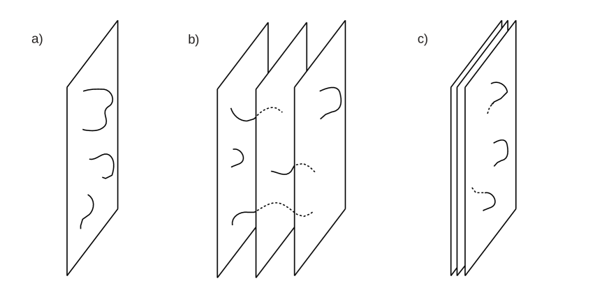
Figure I.1: a) A single D$p$-brane with open strings attached. b) Several parallel D$p$-branes. The open strings can end on different branes. c) A stack of coincident D$p$-branes with enhanced worldvolume gauge symmetry.

D-branes described with open strings :

With $N$ parallel D$p$-branes as in figure I.1 the open string spectrum contains generically $N$ copies of $U(1)$ gauge fields coupled through massive excitations corresponding to strings stretched between different D$p$-branes. In the low energy limit the $N$ worldvolume theories decouple. However if the $N$ D$p$-branes are on top of each other, the lowest modes of open strings stretched between different D$p$-branes become massless and the worldvolume gauge symmetry is enhanced to $U(N)$.

Let’s consider a stack of $N$ coincident D3-branes. The worldvolume $U(N)$ gauge theory from open strings is 4-dimensional and preserve 16 supercharges, corresponding to $\mathcal{N}=4$ supersymmetry. The low-energy limit is obtained by keeping only the massless fields living on the brane and corresponds to the well-known $\mathcal{N}=4$ Super-Yang-Mills gauge theory with gauge group $U(N)$.

Let’s give a rapid description of the theory. It contains only an $\mathcal{N}=4$ vector multiplet $(A^{\mu},\lambda^{a},X^{i})$, so all fields are in the adjoint representation of $U(N)$. The fields charged under the overall $U(1)$ of $U(N)=U(1)\times SU(N)$ (the trace of the matrices) decouple from the theory and we usually consider only the $SU(N)$ gauge theory.
The bosonic fields are a vector field $A^{\mu}$ and 6 real scalars $X^{i}$ corresponding to the position of the stack of D3-branes in the 6 transverse dimensions. The fermionic fields are 4 Weyl fermions $\lambda^{a}$.

The $\mathcal{N}=4$ SYM theory is superconformal,its full supergroup of symmetries is $SU(2,2|4)$. In particular the bosonic symmetries are the spacetime $SO(2,4)\sim SU(2,2)$ combining the 4-dimensional Poincaré symmetries (translations, rotations, Lorentz boosts) and the conformal symmetries (dilatation, special conformal transformations), and the $SO(6)_{R}\sim SU(4)_{R}$ R-symmetry under which the fields transform as $(A^{\mu},\lambda^{a},X^{i})=(\mathbf{1},\mathbf{4},\mathbf{6})$. The fermionic symmetries are 16 Poincaré supersymmetries and 16 conformal supersymmetries.

There is a single complex coupling $\tau=\frac{\theta_{YM}}{2\pi}+\frac{4\pi i}{g_{YM}^{2}}$. The Lagrangian is given by

$$\mathcal{L} =\textrm{Tr}\biggl{\{}-{1\over 2g_{YM}^{2}}F_{\mu\nu}F^{\mu\nu}+{\theta_{YM}\over 8\pi^{2}}F_{\mu\nu}\tilde{F}^{\mu\nu}-\sum_{a}i\bar{\lambda}^{a}\bar{\sigma}^{\mu}D_{\mu}\lambda_{a}-\sum_{i}D_{\mu}X^{i}D^{\mu}X^{i}$$

$$\quad+\sum_{a,b,i}g_{YM}C^{ab}_{i}\lambda_{a}[X^{i},\lambda_{b}]+\sum_{a,b,i}g_{YM}\bar{C}_{iab}\bar{\lambda}^{a}[X^{i},\bar{\lambda}^{b}]+{g_{YM}^{2}\over 2}\sum_{i,j}[X^{i},X^{j}]^{2}\biggr{\}}$$ (I.1.2)

where the constants $C^{ab}_{i}$ and $C_{iab}$ are related to the Clifford Dirac matrices for $SO(6)_{R}\sim SU(4)_{R}$.

The quantum theory enjoys an $SL(2,\mathbb{Z})$ group of dualities under which the $\tau$ parameter transforms as

$$\tau\rightarrow\frac{a\tau+b}{c\tau+d}\quad,\quad ad-bc=1\quad,\quad a,b,c,d\in\mathbb{Z}\ .$$ (I.1.3)

The low energy description of $N$ coincident D3-branes in type IIB string theory contains on one side the low excitations of open strings attached to the D3-branes, which reduce to the 4-dimensional $\mathcal{N}=4$ Super-Yang-Mills conformal gauge theory , and on the other side the low excitations of closed strings which is the 10-dimensional flat space IIB supergravity. In the low energy limit (and string length $l_{s}\rightarrow 0$) these two pieces decouple because the interaction terms are proportional to positive powers of the supergraviy Newton constant (which tends to zero).

D-branes as solitons in 10-dimensions :

The D3-branes have a dual description in string theory as extended objects in 10 dimensions which are sources for supergravity fields. The $\frac{1}{2}$-BPS soliton corresponding to a D$p$-brane in IIB supergravity is the extremal $p$-brane whose metric and dilaton are given by

$$ds^{2} =H(y)^{-\frac{1}{2}}\ dx^{\mu}dx_{\mu}+H(y)^{\frac{1}{2}}\ d\vec{y}^{2}\quad,\quad e^{\Phi}=g_{s}\,H(y)^{\frac{3-p}{4}}$$

$$H(y) =1+\frac{L^{7-p}}{y^{7-p}}\quad,\quad y\equiv\sqrt{\vec{y}^{2}}$$ (I.1.4)

where $x^{\mu}$, $\mu=0,1,\cdots,p$ parametrize the coordinates parallel to the $p$-brane and $\vec{y}=(y^{i})$, $i=p+1,\cdots,9$ are the transverse coordinates. This metric corresponds to a $p$-brane located at $\vec{y}=\vec{0}$. It has $SO(1,p)\times SO(9-p)\times\mathbb{R}^{p+1}$ isometries. The (extremal) $p$-brane solution also has non-vanishing $8-p$-form flux $F_{p+2}$ sourced by the $p$-brane, depending on the harmonic function $H(y)$.

The radius $L$ of the $p$-brane is related to the string coupling $g_{s}$ and the string length $l_{s}=\alpha^{{}^{\prime}\frac{1}{2}}$ through the relation

$$L^{7-p}=(4\pi)^{\frac{5-p}{2}}\Gamma\left(\frac{7-p}{2}\right)\ g_{s}N\,l_{s}^{7-p}\ ,$$ (I.1.5)

where $N$ corresponds to the number of coincident D$p$-branes in the string picture

$$N=\frac{1}{2\kappa_{10}^{2}\,T_{p}}\int_{S^{8-p}}\star F_{p+2}\ ,$$ (I.1.6)

with $2\kappa_{10}^{2}=(2\pi)^{7}l_{s}^{8}g_{s}^{2}$ and $T_{p}=[(2\pi)^{p}l_{s}^{p+1}g_{s}]^{-1}$ is the D$p$-brane tension setting the unit in which the flux is quantized.

Specializing to a stack of $N$ D3-branes, the 10-dimensional backreacted geometry in IIB supergravity is

$$ds^{2} =\left(1+\frac{L^{4}}{y^{4}}\right)^{-\frac{1}{2}}dx^{\mu}dx_{\mu}+\left(1+\frac{L^{4}}{y^{4}}\right)^{\frac{1}{2}}(dy^{2}+y^{2}d\Omega_{5}^{2})$$

$$e^{\Phi} =g_{s}\quad,\quad C\ \textrm{constant}\ ,$$ (I.1.7)

$$F_{5} =(1+\star)dx^{0}dx^{1}dx^{2}dx^{3}d(H(y)^{-1})$$

$$\frac{L^{4}}{l_{s}^{4}} =4\pi g_{s}N\ ,$$

where $d\Omega_{5}^{2}$ is the metric of the unit radius 5-sphere and the axion field $C$ is also non-zero (it is constant).

The coefficient $g_{00}$ of the metric varies along the radial direction $y$ in such a way that the energy of an object at radial position $y$ of the geometry measured by an observer at infinity goes to zero as the object approaches the center $lim_{y\rightarrow 0}E(y)=0$. So the low-energy limit of IIB string theory on this background contains excitations localized near $y=0$, plus the very large wavelength excitations that are those of type IIB flat spacetime supergravity. The two sectors decouple essentially because the large wavelength modes cannot probe the near horizon region.

In the limit $y\rightarrow 0$ the geometry I.1 asymptotes to

$$ds^{2}=L^{2}\left(\frac{1}{u^{2}}\,dx^{\mu}dx_{\mu}+\frac{du^{2}}{u^{2}}+d\Omega_{5}^{2}\right)$$ (I.1.8)

with $u=L^{2}/y$. The limit geometry is regular everywhere. This is actually the famous $AdS_{5}\times S^{5}$ spacetime with equal radius $L$ for the $AdS_{5}$ and $S^{5}$ part. Thus the sector of the theory describing modes localized near $y=0$ or $u=\infty$ is type IIB string theory on $AdS_{5}\times S^{5}$ background.

The last step to reach the Maldacena’s proposal of AdS/CFT correspondence is to identify the two descriptions that we have summarized and to drop the decoupling flat 10-dimensional type IIB supergravity that appears in both descriptions.

The identification of the two reamining pieces leads to the AdS/CFT conjecture :

$\mathcal{N}=4$ Super-Yang-Mills on $\mathbb{R}^{1,3}$ with gauge group $SU(N)$ $\Updownarrow$ Type IIB string theory on $AdS_{5}\times S^{5}$ with radius $L$ .

The parameters of the two theories are identified as follows

$$g_{YM}^{2}=g_{s}\quad,\quad\theta_{YM}=C\quad,\quad\frac{L^{4}}{l_{s}^{4}} =4\pi g_{s}N\ .$$ (I.1.9)

The meaning of this correspondence will be explained in the next subsection.

This form of the conjecture is the strongest as it is meant for any values of $N$ and $g_{YM}$, however it can be tested in practice only in some regimes of parameters where both sides of the correspondence are tractable.
On the SYM side we can use perturbation theory in the weak coupling limit. Allowing for large values of $N$, the effective coupling is $\lambda=g_{YM}^{2}N$, known as the ’t Hooft coupling. In the ’t Hooft limit, where $\lambda$ is fixed and $N$ is large, the perturbation expansion of Feynman diagrams in powers of $\frac{1}{N}$ becomes topological. This means that the diagrams are weighted by $N^{\chi}$, where $\chi$ is the Euler characteristic of the surface on which the diagram can be drawn. The dominant contribution comes for planar diagrams which are the diagrams one can put on a 2-sphere, the next contribution comes from the diagram one can put on a torus, …etc. This topological expansion is similar to the perturbative expansion of closed string amplitudes. In this planar limit, the loop expansion on the sphere is an expansion in powers of $\lambda$ (sigma-model loop expansion), so perturbative computations can be done only for small $\lambda$.

On the string theory side the tractable supergravity description is obtained in the limit of large $L/l_{s}$ and the weak coupling regime correspond to small $g_{s}$. Looking back at I.1.9 it means $g_{s}<<1$ and $g_{s}N>>1$. This is possible only if $N>>1$.

We conclude that the supergravity limit is obtained for $N>>1$ and large $\lambda$, while the weak coupling limit of SYM in the planar limit corresponds to small $\lambda$. These two regimes are incompatible, expaining why the conjectured correspondence is difficult to check. The regime of parameters that is mostly studied is this ’t Hooft limit or planar limit,

$$N\rightarrow\infty\quad,\quad\lambda=g_{s}N\quad\textrm{fixed}\ ,$$ (I.1.10)

for which integrability techniques can be used to study $\mathcal{N}=4$ SYM theory for arbitrary $\lambda$ .

I.2 Elements of correspondence

The first prediction of the AdS/CFT duality is that the global symmetries of both sides should match. This is the case. Let’s compare the bosonic symmetries. The isometry group of $AdS_{5}$ is $SO(2,4)\sim SU(2,2)$ corresponding to the 4-dimensional conformal group of SYM and the isometry group of $S^{5}$ is $SO(6)\sim SU(4)$ corresponding to the R-symmetry of SYM.
The discrete $SL(2,\mathbb{Z})$ symmetry of SYM is mapped to the $SL(2,\mathbb{Z})$ symmetry of type IIB string theory which is preserved by the D3-branes.

The next prediction is that the spectrum of (gauge invariant) operators in SYM theory should be in one-to-one correspondence with the $AdS_{5}$ fields, obtained by expanding the 10d fields in harmonics of $S^{5}$. More precisely the representations of $SU(2,2|4)$ should be mapped and masses $m$ of $AdS_{5}$ fields are related to scalling dimensions $\Delta$ of SYM operators.
It is a very difficult problem to find the match in general, especially because the full IIB string theory spectrum on $AdS_{5}\times S^{5}$ is not known.
Among the gauge multiplets a special role is played by the chiral multiplets or BPS multiplets whose primary operators are anihilated by at least one supercharge. The chiral multiplets thus belong to shorten representations and have the property that their scaling dimension is not renormalized by quantum corrections. The relation to $AdS_{5}$ fields is then easier to find. Generically single trace operators in SYM correspond to single particle (canonical) fields in $AdS_{5}$ ([24, 43]).

The correspondence between $AdS$ fields and gauge theory operator is the key ingredient to relate the two dual theories. In [28, 25] it was argued that the gauge theory could be thought of as living on the boundary at infinity of $AdS_{5}$ with the asymptotic values of the $AdS$ fields $\phi(x^{\mu},u=0)$ playing the role of sources for their dual operator $\mathcal{O}(x^{\mu})$ in the gauge theory. This lead to the crucial GKPW relation

$$\left<e^{\int d^{4}x\,\phi_{0}(x^{\mu})\mathcal{O}(x^{\mu})}\right>_{CFT}=Z_{string}\Big{[}\phi(x^{\mu},u=0)=\phi_{0}(x^{\mu})\Big{]}\ ,$$ (I.2.11)

where the left-hand side is the generating functional of correlation functions for the operator $\mathcal{O}$ in the gauge theory and the right-hand side is the string theory partition function with asymptotic values $\phi_{0}$ for the $AdS$ field $\phi$.

In the supergravity regime the right-hand side can be approximated by the saddle point

$$\left<e^{\int d^{4}x\,\phi_{0}(x^{\mu})\mathcal{O}(x^{\mu})}\right>_{CFT}\simeq e^{-S_{SUGRA}[\phi_{0}]}\ .$$ (I.2.12)

It is then possible to compute gauge theory correlation functions as functional derivatives of the right-hand side with respect to the boundary values $\phi_{0}(x^{\mu})$. The 5-dimensional action used in such a computation comes from dimensional reduction of the $S^{5}$ part and the effective 5d gravitational constant is $G_{5}=\pi/(4N^{2})$.
In the large $N$ limit the computations can be organized in a perturbative expansion in $1/N$, using the so-called Witten diagrams. The endpoints of Witten diagrams lie on the boundary on $AdS$ and the building blocks are boundary-to-bulk propagators and bulk-to-bulk propagators for each AdS field. The perturbative expansion is again a loop expansion.

The simplest prediction from the GKPW relation I.2.11 is the equality between the free energy $F_{CFT}\equiv-\log|Z_{CFT}|$ and the action $S_{sugra}$ evaluated on the dual supergravity background $g_{\mu\nu}^{(0)},\phi^{(0)},...$

$$F_{CFT}=S_{sugra}[g_{\mu\nu}^{(0)},\phi^{(0)},...]\ .$$ (I.2.13)

The UV divergences one encounters on the gauge theory side have a counterpart on the gravity side as IR divergences related to the infinite size of the AdS spacetime. Imposing a UV cutoff in the gauge theory translates into imposing a radial cut-off in AdS. The regularization techniques of the gravity computations go under the name of holographic renormalization [27, 44, 45] and amounts to adding universal covariant boundary counterterms to the action. We will review the holographic renormalization of the pure gravity action in the next subsection and we will use the results for the regularized (euclidean) AdS volume in the core of the presentation.

Generalizations of the AdS/CFT correspondence

Up to now we have only presented the original AdS/CFT correspondence between $\mathcal{N}=4$ SYM gauge theory and Type IIB string theory on $AdS_{5}\times S^{5}$. One of its most surprizing feature is that it relates a theory without gravity and a theory containing gravity. Moreover in the supergravity regime one can match classical gravity computations with quantum computations on the gauge theory side. These general features are expected to hold for more general dualities involving a $d$-dimensional CFT and quantum theory of gravity on $AdS_{d+1}\times K$ background, where $K$ is a compact space whose dimension is $9-d$ for string theories and $10-d$ for the (mysterious) M-theory.

A first generalization consists in orbifolding the 5-sphere to obtain a duality between Type IIB string theory on $AdS_{5}\times S^{5}/\Gamma$ and 4d SYM with $\mathcal{N}=4,2,1,0$ supersymmetry depending on the orbifold [46]. A simple example is the duality between $\mathcal{N}=4$ SYM with gauge group $SO(N)$ or $Sp(N/2)$ and IIB string theory on $AdS_{5}\times\mathbb{R}\mathbb{P}^{5}$ [47], with $\mathbb{R}\mathbb{P}^{5}=S^{5}/\mathbb{Z}_{2}$ the 5d real projective space.

For $AdS_{4}/CFT_{3}$ dualities, which are the main topic here, the most famous and well-understood example relates M-theory on $AdS_{4}\times S^{7}/\mathbb{Z}_{k}$ and the so-called ABJM gauge theory [1]. Let’s describe it in detail as it is of particular interest for us.

The gauge theory side is a 3-dimensional SCFT with $\mathcal{N}=6$ supersymmetry with $U(N)\times U(N)$ gauge group with level $k$ and $-k$ Chern-Simons terms for the two unitary nodes respectively. The matter content is made of two ($\mathcal{N}=4$) bifundamental hypermultiplets, that is one $(\mathbf{N},\bar{}\mathbf{N})$ chiral multiplet and one $(\bar{}\mathbf{N},\mathbf{N})$ chiral multiplet for each. The Lagrangian has also a $\mathcal{N}=4$ superpotential. The theory has a priori only $\mathcal{N}=3$ supersymmetry due to the Chern-Simons terms, however one can show the presence of an $SO(6)_{R}$ R-symmetry ensuring $\mathcal{N}=6$ supersymmetry.
When $k=1$ or $k=2$ the supersymmetry is enhanced to $\mathcal{N}=8$ and the theory is known as the BLG theory [48]. The ’t Hooft coupling is $\lambda=N/k$ so that the theory is weakly coupled when $N/k<<1$.

The ABJM SCFT is supposed to be the low-energy worldvolume description of a stack of $N$ M2-branes placed at the tip of a $\mathbb{C}^{4}/\mathbb{Z}_{k}$ orbifold in M-theory.
In the regime $N>>k^{5}$ the theory is correctly described by 11-dimensional supergravity on $AdS_{4}\times S^{7}/\mathbb{Z}_{k}$ with metric

$$ds^{2} =\frac{L^{2}}{4}\,ds^{2}_{AdS_{4}}+L^{2}\,ds^{2}_{S^{7}/\mathbb{Z}_{k}}$$ (I.2.14)

$$L^{6} =2^{5}\pi^{2}kN\,l_{p}^{6}$$

where $l_{p}$ is the eleven-dimensional Planck length. The unit seven-sphere can be embedded in $\mathbb{C}^{4}$ as $|z_{1}|^{2}+|z_{2}|^{2}+|z_{3}|^{2}+|z_{4}|^{2}=1$ and the orbifold action is $z_{i}\sim e^{\frac{2i\pi}{k}}\,z_{i}$ (which has no fixed point). The 11d supergravity solution also has $N$ units of four-form flux along the $AdS_{4}$ factor.
$S^{7}/\mathbb{Z}_{k}$ can be described as an $S^{1}$ fibered of $\mathbb{C}\mathbb{P}^{3}$ with the orbifold acting only on the $S^{1}$ angle. When $N^{1/5}<<k<<N$ the $S^{1}$ circle shrinks and the theory is well-described as Type IIA string theory on $AdS_{4}\times\mathbb{C}\mathbb{P}^{3}$

$$ds^{2}_{IIA} =R^{2}_{str}\left(\frac{1}{4}\,ds^{2}_{AdS_{4}}+ds^{2}_{\mathbb{C}\mathbb{P}^{3}}\right)$$ (I.2.15)

$$R^{2}_{str} =2^{5/2}\pi(N/k)^{\frac{1}{2}}\,l_{s}^{2}.$$

The ABJM correspondence admits a generalization to $U(N)_{k}\times U(M)_{-k}$ gauge group with $|M-N|\leq|k|$, corresponding to have discrete torsion flux of the 3-form potential $C^{3}$ along $S^{3}/\mathbb{Z}_{k}\subset S^{7}/\mathbb{Z}_{k}$ in M-theory or discrete $B_{2}$ holonomy along $\mathbb{C}\mathbb{P}^{1}\subset\mathbb{C}\mathbb{P}^{3}$ in type IIA [49].

T-dualizing to Type IIB string theory the ABJM gauge theory can be thought of as the low-energy theory living on D3-branes in a brane configuration where the $N$ D3-branes wrap a circle (T-duality circle) and cross a NS5-brane and a $(1,k)$ 5-brane. The generalization includes $M-N$ additional D3-branes stretched between the 5-branes, as in figure I.2. This is an example of circular quiver. We will encounter this kind of brane configurations all along the presentation and will give much more details.

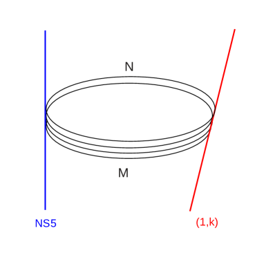
Figure I.2: IIB Brane configuration for ABJ(M) gauge theory with $M>N$. $N$ D3-branes wrap a circle and cross a NS5-brane and a $(1,k)$ 5-brane. $M-N$ D3-branes are stretched between the 5-branes.

Today many AdS/CFT duals have been proposed in various dimensions . One remaining challenge is to understand the mysterious $\mathcal{N}=(2,0)$ 6-dimensional SCFT that is supposed to live on the worldvolume of a stack of $N$ M5-branes in M-theory.

The AdS/CFT correspondence is actually expected to hold for spacetime whose metric is only asymptotically AdS (AAdS), the generic case being a blackhole with asymptotic AdS metric (AdS blackhole), which is related to a quantum field theory at finite temperature. The deviation from AdS spacetime along the radial direction when going from the boundary to the bulk is now understood as the RG flow from a UV theory ($\mathcal{N}=4$ SYM in general) perturbed by a relevant operator to the IR. We refer to the reviews [50, 51] for presentations of some extensions of AdS/CFT correspondence.

I.3 Holographic renormalization of the gravity action

In this subsection we summarize the derivation of the renormalized pure gravity action in Eucildean AdS spacetime. A good review presenting the holographic renormalization techniques is [45]. Our very brief presentation is based on the review [52] (section 5), which adresses the question of the regularization of the euclidean $AdS$ gravity action in great details. Some of the original papers are [27, 44, 53].

The gravitational Einstein-Hilbert action in Euclidean $n+1$ dimensional space with cosmological constant $\Lambda$ is the sum of a bulk term and a boundary term named Gibbons-Hawking term

$$S\quad =S_{bulk}+S_{GH}$$

$$S_{bulk} =-\frac{1}{16\pi G_{N}}\int_{M}d^{n+1}x\,|G|^{\frac{1}{2}}(R-2\Lambda)$$ (I.3.16)

$$S_{GH} =-\frac{1}{8\pi G_{N}}\int_{\partial M}d^{n}x\,K\,|\gamma|^{\frac{1}{2}}$$

where $G_{N}$ is the Newton’s constant, $G_{\mu\nu}$ is the metric on the $n+1$-dimensional manifold $M$, $\partial M$ is the boundary of $M$, $\gamma_{ij}$ is the induced metric on $\partial M$ and $K$ is the extrinsic curvature of $\partial M$ satisfying $|\gamma|^{\frac{1}{2}}K=\mathcal{L}_{\vec{s}}|\gamma|^{\frac{1}{2}}$ with $\mathcal{L}_{\vec{s}}$ the Lie derivative along the unit vector $\vec{s}$ normal to $\partial M$.

The cosmological constant for $AdS_{n+1}$ space with radius $L$ is

$$\Lambda=-\frac{n(n-1)}{2\,L^{2}}$$ (I.3.17)

and the Ricci tensor and scalar are given by

$$R_{\mu\nu} =-\frac{n}{L^{2}}\ G_{\mu\nu}\quad,\quad R=-\frac{n(n+1)}{L^{2}}\ .$$ (I.3.18)

Both terms in the action I.3 diverge when evaluated on (Euclidean) AdS space because of its infinite size.

A metric asymptotically AdS can be written

$$ds^{2} =L^{2}\left(\frac{du^{2}}{u^{2}}+\frac{1}{u^{2}}\,g_{ij}(u^{2},x)\,dx^{i}dx^{j}\right)$$ (I.3.19)

and the $g_{ij}$ can be expanded in a power series of $u^{2}$ near the boundary $u=0$ of $AdS_{n+1}$

$$g_{ij}(u^{2},x) =g^{(0)}_{ij}(x)+u^{2}g^{(2)}_{ij}(x)+\cdots+u^{n}\left(g^{(n)}_{ij}(x)+h^{(n)}_{ij}(x)\log(\sqrt{u})\right)+\cdots$$ (I.3.20)

where the term $h^{(n)}$ is present only for even $n$. The coefficients $g^{(2)},g^{(4)},\cdots,g^{(n-2)}$ (or $g^{(n-1)}$) and $h^{(n)}$ can be expressed in terms of $g^{(0)}$ recursively by plugging I.3.20 in Einstein’s equations. $g^{(n)}$ is independent of $g^{(0)}$ and is related to the one-point function of the boundary stress-energy tensor.

As mentioned above the regularization consists in truncating the manifold $M$ to the manifold $M_{\epsilon}$ with $u\geq\epsilon$, so that the boundary $\partial M_{\epsilon}$ is at finite distance.

Evaluating the action I.3 on $M_{\epsilon}$ yields a regulated action with the structure

$$S_{\epsilon}\ =\frac{L^{n-1}}{16\pi G_{N}}\int d^{n}x\,\sqrt{g^{(0)}}\left(\epsilon^{-n}a_{(0)}+\epsilon^{-n+2}a_{(2)}+\cdots+\epsilon^{-2}a_{(n-2)}-2\log(\epsilon)a_{(n)}\right)\quad+O(\epsilon^{0})$$

$$a_{(0)}=2(1-n)$$

$$a_{(2)}=-\frac{(n-4)(n-1)}{n-2}\ \textrm{Tr}\left(g^{(0)-1}g^{(2)}\right)\quad(n>2)$$ (I.3.21)

$$a_{(4)}=\cdots\quad(n>4)$$

where the logarithm appears only for even $n$.

The procedure consists simply in adding a counterterm equal to minus the divergent part of the action as $\epsilon\rightarrow 0$ and rewrite it in terms of covariant quantities on the boundary with metric $\gamma$

$$S_{ct} =-\frac{L^{n-1}}{16\pi G_{N}}\int d^{n}x\,\sqrt{g^{(0)}}\left(\epsilon^{-n}a_{(0)}+\epsilon^{-n+2}a_{(2)}+\cdots+\epsilon^{-2}a_{(n-2)}-2\log(\epsilon)a_{(n)}\right)$$

$$=\frac{1}{8\pi G_{N}}\int d^{n}\sqrt{\gamma}\left(\frac{n-1}{L}+\frac{L}{2(n-2)}\,R[\gamma]+\cdots+2a_{(n)}[\gamma]\log(\epsilon)\right)\ .$$ (I.3.22)

The total action on $M_{\epsilon}$ is then

$$S_{reg}=S_{bulk}+S_{GH}+S_{ct}\ .$$ (I.3.23)

It is finite in the limit $\epsilon\rightarrow 0$ by construction, so the regularized action is computed using I.3.23 at finite $\epsilon$ and then putting $\epsilon=0$.

This procedure can be applied to Euclidean AdS space in several coordinate systems with a variety of topological boundaries leading to different results (see [44]). For our purpose we can extract from the action a regularized $AdS$ volume, which is directly proportional to the pure gravity AdS action. Let’s just mention the result that we will use, namely the regularized volume of pure $AdS_{4}$ Euclidean space with the 3-sphere $S^{3}$ as conformal boundary

$$\textrm{Volume}(AdS_{4})_{reg} =\frac{16\pi G_{N}\,L^{2}}{6}\ S_{reg}\ =\ \frac{4}{3}\pi^{2}L^{4}\ .$$ (I.3.24)

Chapter II 3d $\mathcal{N}=4$ quivers and brane realizations

In this chapter we describe the class of Super-Conformal field theories for which we will propose Type IIB holographic duals. These gauge theories arise as strongly interacting infrared fixed points of 3d quiver gauge theories with $\mathcal{N}=4$ supersymmetries. The relevant supergroup of symmetries is $OSp(4|4)$. The bosonic symmetries are the 3-dimensional conformal group $SO(2,3)\sim USp(4)$ and the $SU(2)_{L}\times SU(2)_{R}\sim SO(4)$ R-symmetry.

As in the original setup of Maldacena (see section I.1), they can be understood as the low energy limit of the worlvolume theories of D3-branes, but this time the brane configurations involve also D5-branes and NS5-branes. The relation to the brane configurations will prove crucial when we come to the supergravity duals in the next chapter.

II.1 $\mathcal{N}=4$ supersymmetric gauge theories in 3 dimensions

The following brief presentation of $\mathcal{N}=4$ $d=3$ (super-conformal) gauge theories and their known properties is freely inspired by [54, 13, 55, 56, 57, 58, 15, 59, 33, 60, 61, 52, 62], which also describe many interesting features about the dynamics of the $\mathcal{N}=2$ theories.

II.1.1 $\mathcal{N}=4$ supersymmetry in 3 dimensions and Lagrangian

The $\mathcal{N}=4$ supersymmetry algebra in 2+1 dimensions has 8 real supercharges. This is four times the minimal supersymmetry (2 supercharges : $\mathcal{N}=1$) and half the maximal amount (16 supercharges : $\mathcal{N}=8$). The algebra can be obtained by reducing the 4-dimensional $\mathcal{N}=2$ supersymmetry algebra to 3 dimensions. It can be written in terms of 4 real spinor generators $Q^{A}$, $A=1,2,3,4$.

$$\{Q_{\alpha}^{A},Q_{\beta}^{B}\}=2\ \sigma^{\mu}_{\alpha\beta}\,\delta^{AB}\,P_{\mu}+2\,\epsilon_{\alpha\beta}Z^{AB}\ ,$$ (II.1.1)

with $A,B=1,2,3,4$ , $\mu=0,1,2$, $\{\sigma^{\mu}\}$ are a set of generators of the 3-dimensional Clifford algebra, $\epsilon_{\alpha\beta}$ is a conventional anti-hermitian matrix used for lowering spinor indices and $Z^{AB}$ is a real antisymmetric matrix of central charges that commutes with all the generators of the algebra. $Z^{AB}$ has two independent components, that are derived from the real central charge in $d=4$ $\mathcal{N}=2$ and the momentum generator $P^{3}$ in the reduced dimension.

The super-algebra has a $SU(2)_{L}\times SU(2)_{R}\simeq SO(4)$ group of R-symmetry (automorphisms of the algebra) that rotates the supercharges $Q^{A}$ as the $\mathbf{4}$ of $SO(4)$.

Generally the super-algebra for $\mathcal{N}$ supersymmetry is the same with $A,B=1,2,\cdots,\mathcal{N}$ and the R-symmetry group that rotates the supercharges is $SO(\mathcal{N})$.

The superconformal extension is given by the super-group $OSp(4|4)$. It contains the conformal extension of the Poincaré group in 3 dimensions $SO(2,3)\simeq USp(4)$ and it has 8 additional real conformal supercharges, so 16 (real) supercharges in total. In Euclidean signature the conformal group is $SO(1,4)\simeq USp(2,2)$ and the super-conformal group is named $OSp(4|2,2)$.

$\mathcal{N}=4$ $d=3$ of quiver gauge theories contain vector multiplets and hypermultiplets, defined in turn in terms of $\mathcal{N}=2$ multiplets, for which there is a superspace formulation.

The field contents of the $\mathcal{N}=4$ vector multiplet and hypermultiplet are summarized in table II.1, with their transformation under the R-symmetry $SU(2)_{L}\times SU(2)_{R}$ and gauge group $G$ indicated. The notations for the various fields and auxiliary fields are pretty standard and should not bring confusion. All fermions are two-component complex spinors. The scalar $\sigma$ and auxiliary scalar $D$ in the vector multiplet are real, while the scalars “$\phi$” and auxiliary scalars “$F$” in each $\mathcal{N}=2$ chiral multiplet are complex.

$\mathcal{N}=4$	$\mathcal{N}=2$ (superfield)	Components	$SU(2)_{L}\times SU(2)_{R}$	$G$
vector	vector	$A_{\mu}$		adjoint
multiplet	multiplet ($V$)	$\lambda_{\alpha}$
		$\sigma$	$\big{\{}\sigma,Re\varphi,Im\varphi\big{\}}\quad\textrm{in}\quad\left(1,0\right)$
		$D$	$\big{\{}\lambda_{\alpha},\xi_{\alpha}\big{\}}\quad\textrm{in}\quad\left(\frac{1}{2},\frac{1}{2}\right)$
	chiral	$\varphi$	$\big{\{}D,ReF_{\Phi},ImF_{\Phi}\big{\}}\quad\textrm{in}\quad\left(0,1\right)$
	multiplet ($\Phi$)	$\xi_{\alpha}$
		$F_{\Phi}$
hyper	chiral	$\phi$		$R$
multiplet	multiplet ($\phi$)	$\psi_{\alpha}$
		$F$	$\big{\{}\phi^{{\dagger}},\tilde{\phi}\big{\}}\quad\textrm{in}\quad\left(0,\frac{1}{2}\right)$
	chiral	$\tilde{\phi}$	$\big{\{}\psi_{\alpha},\tilde{\psi}_{\alpha}\big{\}}\quad\textrm{in}\quad\left(\frac{1}{2},0\right)$	$R^{*}$
	multiplet ($\tilde{\phi}$)	$\tilde{\psi}_{\alpha}$	$F,\tilde{F}\quad$ integrated out
		$\tilde{F}$

Table II.1: Field content and R-charges of the $\mathcal{N}=4$ supermultiplets.

A $\mathcal{N}=2$ chiral multiplet can be recast in terms of a chiral superfield $\Phi$ with $\bar{D}_{\alpha}\Phi=0$

$$\Phi=\phi+\sqrt{2}\theta\,\psi+\theta^{2}F$$ (II.1.2)

with $\theta$ a two components grassmann variable.
The $\mathcal{N}=2$ vector multiplet can be recast in terms of a real superfield $V$ with $V^{\dagger}=V$, which reads in Wess-Zumino gauge

$$V=-\theta^{\alpha}\sigma^{\mu}_{\alpha\beta}\bar{\theta}^{\beta}A^{\mu}-\theta\bar{\theta}\sigma+i\theta\theta\bar{\theta}\bar{\lambda}-i\bar{\theta}\bar{\theta}\theta\lambda+\frac{1}{2}\theta\theta\bar{\theta}\bar{\theta}D\ ,$$ (II.1.3)

where the components are adjoint valued matrices. The chiral field strength is defined via $W_{\alpha}=-\frac{1}{4}\bar{D}\bar{D}e^{-V}D_{\alpha}e^{V}$.

The flat space euclidean action for the $\mathcal{N}=4$ quiver theories is composed of the following $\mathcal{N}=2$ superspace pieces.

• A Yang-Mills action for each node in the gauge group. The gauge couplings for the different nodes need not be the same but all flow to strong coupling in the IR.

  $$S_{vector}^{\mathcal{N}=4} =\frac{1}{g^{2}}\int d^{3}xd^{2}\theta d^{2}\bar{\theta}\ \textrm{Tr}\left(W_{\alpha}^{2}-\Phi^{\dagger}e^{2V}\Phi\right)+h.c.$$

  where $W$ is the chiral field strength of the $\mathcal{N}=2$ vector superfield $V$ and $\Phi$ is the adjoint chiral superfield. In components we have
  $S_{vector}^{\mathcal{N}=4}=S_{vector}^{\mathcal{N}=2}+\frac{1}{g^{2}}\,S_{adj\ chiral}^{\mathcal{N}=2}$ with

  $$S_{vector}^{\mathcal{N}=2} =\frac{1}{2g^{2}}\int d^{3}x\ \textrm{Tr}\left(\frac{1}{2}F_{\mu\nu}F^{\mu\nu}+D_{\mu}\sigma D^{\mu}\sigma+D^{2}+i\bar{\lambda}\gamma^{\mu}D_{\mu}\lambda+i\bar{\lambda}[\sigma,\lambda]\right)$$

  $$S_{chiral}^{\mathcal{N}=2} =-\int d^{3}x\ \left(D_{\mu}\bar{\phi}D^{\mu}\phi+\bar{\phi}\sigma^{2}\phi+i\bar{\phi}D\phi+\bar{F}F-i\bar{\psi}\gamma^{\mu}D_{\mu}\psi+i\bar{\psi}\sigma\psi+i\bar{\psi}\lambda\phi-i\bar{\phi}\bar{\lambda}\psi\right)$$

• A kinetic term and gauge coupling for each hypermultiplet.

  $$S_{hyper}^{\mathcal{N}=4}=-\int{d^{3}x{d^{2}}\theta{d^{2}}\bar{\theta}}\sum\limits_{matter}{({\phi^{\dagger}}{e^{2V}}\phi}+{{\tilde{\phi}}^{\dagger}}{e^{-2V}}\tilde{\phi})$$

  where $\phi,\tilde{\phi}$ are two chiral superfields in conjugate representations.

• A $\mathcal{N}=4$ superpotential.

  $$S_{spot}^{\mathcal{N}=4}=-i\sqrt{2}\int d^{3}xd^{2}\theta\ \sum\limits_{matter}(\tilde{\phi}\Phi\phi)+h.c$$

  where the sum runs over all matter charged under the gauge symmetry associated with $\Phi$.

The gauge theories enjoy two possible deformations :

• Real and complex mass terms for the hypermultiplets. The 3 real parameters transform as a triplet of $SU(2)_{R}$ and can be viewed as the lowest components of a background $\mathcal{N}=4$ abelian vector multiplet coupled to the flavor symmetry currents.

  $$S_{mass}^{\mathcal{N}=4}=-\int d^{3}xd^{2}\theta d^{2}\bar{\theta}\sum\limits_{matter}(\phi^{{\dagger}}e^{2{V_{m}}}\phi+\tilde{\phi}^{{\dagger}}e^{-2{V_{m}}}\tilde{\phi})-\left(i\sqrt{2}\int d^{3}xd^{2}\theta\sum\limits_{matter}(\tilde{\phi}{\Phi_{m}}\phi)+h.c\right)$$

  The Lagrangian (with the complex mass to rotated to zero) is then obtained by setting $V_{m}\propto m\bar{\theta}\theta$ and $\Phi_{m}=0$, where $m$ is the real mass parameter. This ensures the vanishing of the fermion variations of the background multiplet. In components it reads

  $$S_{mass}^{\mathcal{N}=2}(\phi,m)=\int d^{3}x\ \left(D_{\mu}\bar{\phi}D^{\mu}\phi+m^{2}\,\bar{\phi}\phi+\bar{F}F-i\bar{\psi}\gamma^{\mu}D_{\mu}\psi+i\,m\,\bar{\psi}\psi\right)$$

  and $S_{mass}^{\mathcal{N}=4}=S_{mass}^{\mathcal{N}=2}(\phi,m)+S_{mass}^{\mathcal{N}=2}(\tilde{\phi},-m)$.

• Fayet-Iliopoulos (FI) terms for the $U(1)$ factors of the gauge group. The three real parameters transform as a triplet of $SU(2)_{L}$. They can be viewed as the lowest components of a background twisted $\mathcal{N}=4$ abelian vector multiplet coupled to the topological currents associated with the $U(1)$ gauge factors by a $BF$ type coupling.

  $$S_{FI}^{\mathcal{N}=4}=\int d^{3}xd^{2}\theta d^{2}\bar{\theta}\ \textrm{Tr}\left(\Sigma\,\hat{V}_{FI}\right)\ +\ \int d^{3}xd^{2}\theta\ \textrm{Tr}\left(\Phi\hat{\Phi}_{FI}+h.c\right)$$

  where the Tr picks out the central $U(1)$ factor of the gauge group (we have a FI deformation for each gauge node of a quiver theory). Again the deformed Lagrangian (with two deformation parameters rotated to zero) is obtained by setting ${\hat{V}}_{FI}\propto\eta\bar{\theta}\theta,\hat{\Phi}_{FI}=0$, leading to

  $$S_{FI}=i\,\eta\ \int d^{3}x\ D$$

It is also possible to add a Chern-Simons term of level $k\in\mathbb{Z}$ to the action, which breaks $\mathcal{N}=4$ to $\mathcal{N}=3$ :

$$S_{CS}^{\mathcal{N}=3} =S_{CS}^{\mathcal{N}=2}-\frac{k}{8\pi}\int d^{3}xd^{2}\theta\textrm{Tr}\left(\Phi^{2}+h.c.\right)$$ (II.1.4)

$$S_{CS}^{\mathcal{N}=2} =\frac{k}{4\pi}\int d^{3}x\ \textrm{Tr}\left(\epsilon^{\mu\nu\rho}\left(A_{\mu}\partial_{\nu}A_{\rho}+\frac{2i}{3}A_{\mu}A_{\nu}A^{\rho}\right)-\lambda\bar{\lambda}+2D\sigma\right)$$

where $\Phi$ is an adjoint chiral superfield.

To close this introductory part, we mention the duality between abelian vector field and scalar field in 3 dimensions, represented by the relation

$$F_{\mu\nu}=\epsilon_{\mu\nu\sigma}\partial^{\sigma}\gamma\ ,$$ (II.1.5)

where $\gamma$ is a periodic ($\gamma\simeq\gamma+g_{YM}$) real scalar called dual photon. The whole $\mathcal{N}=2$ vector multiplet can be dualized to a chiral multiplet with lowest component $\sigma+i\gamma$ (see [56]).

II.1.2 Mirror symmetry

The 3d $\mathcal{N}=4$ quiver gauge theories moduli space of vacua of the quiver gauge theories is obtained by minimizing the scalar potential in the Lagrangian. This implies solving the D-term and F-term constraints, which are scalar potentials arising after integrating out the auxiliary scalars $D$ and $F$. Generically the moduli space is decomposed into two branches [57, 58, 13] :

• The Coulomb branch corresponding to giving vevs to the scalars $\phi_{i}$, $i=1,2,3$ in the vector multiplet preserving the vanishing potential condition $\sum_{i<j}Tr([\phi_{i},\phi_{j}]^{2})=0$. The scalar vevs $<\phi_{i}>$ are given by diagonal matrices breaking the gauge group to its maximal torus $U(1)^{r}$. The full Coulomb branch is obtained by giving vevs to the $r$ dual photons associated to the surviving $r$ abelian vector fields. The Coulomb branch (of $\mathcal{N}=4$ theories) is a hyper-Kähler manifold of (real) dimension $4r$. The metric on the Coulomb branch receives quantum corrections due to 3-dimensional monopoles (also named instantons in the litterature as they are codimension 3 solutions of BPS equations), but its dimension is unaffected.

• The Higgs branch corresponding to giving vevs to the scalars $\phi_{i}$, $i=1,2,3,4$ in the hyper-multiplets. The equations defining the Higgs branch may allow for a complete gauge symmetry breaking. For instance for a gauge group $U(N_{c})$ with $N_{f}$ hypermultiplets the conditions for complete higgsing is $N_{f}\geq 2N_{c}$. When a complete higgsing is not possible, one expect that the infrared theory contains free vector multiplets ([11]). The Higgs branch (of $\mathcal{N}=4$ theories) is a hyper-Käler manifold. Promoting the gauge coupling constant to a superfield, one can show that the scalars of the superfield do not transform under the $SU(2)_{R}$ R-symmetry, so that they can appear only in the Coulomb branch (see [63, 58]). It implies that the Higgs branch does not receive quantum corrections.

Mirror symmetry ([58]) is a duality between $d=3$ $N=4$ supersymmetric gauge theories, with different gauge groups and matter contents, which exchanges the Higgs branch and Coulomb branch of vacua, exchanges the mass and Fayet-Iliopoulos parameters and the $SU(2)_{L}$ and $SU(2)_{R}$ R-symmetries. This implies that the quantum corrections of the Coulomb branch are contained in the purely classical Higgs branch of the mirror dual theory ([13, 64]).

The 3d Yang-Mills gauge theories are super-renormalizable : they flow to free theories in the ultra-violet. Conversely they are infinitely strongly coupled in the infrared where the Lagrangian description breaks down. The prediction from mirror symmetry is that the IR strongly interacting fixed points of mirror theories arising from the RG flow at the intersection/origin of the Coulomb and Higgs branches are the same SCFTs. By deforming the SCFTs with mass and Fayet-Iliopoulos parameters (that are not renormalized due to supersymmetry) one gets a duality between non-conformal supersymmetric theories.

One prediction of mirror symmetry is the emergence of global symmetries at the super-conformal fixed point (intersection of Higgs and Coulomb branch). The SCFTs have global non-abelian flavor symmetries, which should appear as different global symmetries in the IR limit of the dual theory. More precisely the gauge theories have abelian topological global symmetries associated with each $U(1)$ factor in the gauge group (one for each $U(N_{i})$ node), with conserved current $\star F$. At the super-conformal fixed point the topological symmetries can be enhanced to non-abelian symmetries, that are exchanged with the flavor symmetries under mirror symmetry.

The fact that the SCFTs are infinitely strongly coupled makes it difficult to test mirror symmetry and until recently the only checks concerned moduli spaces. The techniques of localization of path integrals on the 4-sphere developped in [65] and pursued in [15] for supersymmetric theories on the 3-sphere have rendered possible to compute supersymmetric observables by reducing the whole path integral to finite dimensional matrix integrals (matrix models). The resulting matrix models do not depend on the Yang-Mills coupling and are consequently directly related to the observables of the IR fixed points.

Using the matrix models [59] provided further evidences of mirror symmetry by matching partition functions of mirror pairs, under the exchange of mass and FI parameters.

While we were completing this manuscript, [66] appeared which uses mirror symmetry for 3d $\mathcal{N}=4$ linear quivers and the map between their space of vacua and the eigenvalues of quantum integrable spin chain Hamiltonians to derive new dualities between these integrable models, called bispectral dualities.

On the holographic side that we study, mirror symmetry will be naturally implemented by the S-duality of type IIB string theory.

II.1.3 Matrix models

As we will use the matrix models obtained from the localization of path integrals of $\mathcal{N}=4$ gauge theories on the 3-sphere, we give here a short summary of these matrix models, obtained in [15] for $\mathcal{N}=2$ theories. Further details about $d=3$ supersymmetric gauge theories on $S^{3}$ can be found in [60]. A good review of the localization on $S^{3}$ is [52].

The localisation on $S^{3}$ of the partition function $Z_{S^{3}}$ reduces the whole path integral to an integration over the Cartan subalgebra of the gauge group, divided by the order of the Weyl group $|\mathcal{W}|$. We give here explicit formulas for a $U(N)$ gauge group.

$$Z_{S^{3}} =\frac{1}{|\mathcal{W}|}\int_{\textrm{Cartan}}d\sigma\ \Big{(}...\Big{)}\ =\ \frac{1}{N!}\int\prod_{i}^{N}d\sigma_{i}\ \Big{(}...\Big{)}\ .$$ (II.1.6)

The integrand (the dots in (II.1.6)) is a product of several contributions .

The $\mathcal{N}=4$ vector multiplet gives a factor

$$\textrm{det}_{\rm Adj}\Big{(}\textrm{sh}(\sigma)\Big{)}\ =\ \prod_{i<j}^{N}\textrm{sh}(\sigma_{i}-\sigma_{j})^{2}\ ,$$ (II.1.7)

a hyper-multipet in a representation $R$ of the gauge group with mass $m$ gives a factor

$$\textrm{det}_{R}\Big{(}\frac{1}{\textrm{ch}(\sigma-m)}\Big{)} =\prod_{j}^{N}\textrm{ch}(\sigma_{j}-m)\ \textrm{for the fundamental rep. of }\,U(N)$$ (II.1.8)

$$=\prod_{i,j}^{N,M}\textrm{ch}(\sigma_{i}-\tilde{\sigma}_{j}-m)\ \textrm{for the bifundamental rep. of}\,U(N)\times U(M)\ ,$$

a Chern-Simons term with level $k$ contributes a factor

$$\textrm{det}_{F}\Big{(}e^{i\pi k\sigma^{2}}\Big{)}\ =\ e^{i\pi k\sum_{j}^{N}\sigma_{j}^{2}}\ ,$$ (II.1.9)

and a Fayet-Iliopoulos deformation $\eta$ produces a term

$$\textrm{det}_{F}\Big{(}e^{2i\pi\eta\sigma}\Big{)}\ =\ e^{2i\pi\eta\sum_{j}^{N}\sigma_{j}}\ .$$ (II.1.10)

Here $\det_{R}$ (and below $\textrm{Tr}_{R}$) is the the determinant (the trace) in the representation $R$. The indices $F$ and ${\rm Adj}$ will refer to fundamental and adjoint representations respectively.

To close this introduction we would like to mention that the localization techniques have been applied to the richer cases of $d=3$ $\mathcal{N}=2$ gauge theories with non-canonical R-charge assignments [33, 60] and on the squashed 3-sphere [61], and that the superconformal index (partition function on $S^{1}\times S^{2}$) was also studied in [67, 68, 69, 70].

We also mention that recently $\mathcal{N}=4$ Seiberg-like dualities relating the quiver with $U(N_{c})$ gauge group and $N_{f}$ hypermultiplets, with $N_{f}\geq 2N_{c}$, and the quiver with $U(N_{f}-N_{c})$ gauge group and $N_{f}$ hypermultiplets plus $N_{f}-2N_{c}$ free hypermultiplets (corresponding to monopoles operators with special R-charges asignments) have been proposed in [71]. Further details and comments on this duality immediatly followed in [66, 72].
This duality is perfectly consistent with the holographic descriptions that we propose in this presentation, in the sense that we have only one supergravity solution for dual theories.

II.2 Linear and circular quivers

The three-dimensional $\mathcal{N}=4$ superconformal field theories considered in this paper arise as non-trivial infrared fixed points of three-dimensional quiver gauge theories with $\mathcal{N}=4$ supersymmetries. Their field content and their microscopic Lagrangians are succinctly summarized by a quiver diagram [73]. In our case the diagrams will have either linear or circular topology (see figures II.1 and II.2). We refer to the corresponding quivers as linear and circular respectively.

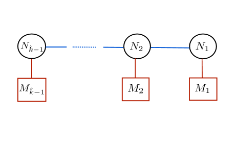
Figure II.1: A linear quiver with $\hat{k}-1$ gauge-group factors $U(N_{1})\times U(N_{2})\times\cdots$. The red boxes indicate the numbers of hypermultiplets in the fundamental representation of each gauge-group factor.

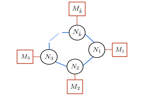
Figure II.2: A circular quiver with $\hat{k}$ gauge-group factors. The $U(N_{i})$ theories interact via bifundamental hypermultiplets (the blue lines) which form a circular chain, as opposed to the linear chain of figure 1.

The quiver gauge theories contain a vector multiplet for each unitary node of the gauge group

$$U(N_{1})\times U(N_{2})\times...\ U(N_{i})\times...\,.$$ (II.2.11)

Moreover, these theories contain a hypermultiplet transforming in the bifundamental representation of each consecutive pair of gauge groups $U(N_{i})\times U(N_{i+1})$. For linear quivers $1\leq i\leq\hat{k}-2$, while for the circular quivers $1\leq i\leq\hat{k}$ with the convention that $U(N_{\hat{k}+1})\equiv U(N_{1})$. Finally, there are $M_{i}$ hypermultiplets in the fundamental representation of the group $U(N_{i})$.

Irreducible infrared SCFTs

A central question about the dynamics of these gauge theories is to understand the nature of the fixed point of the renormalization group in the infrared. Since massive fields decouple in the infrared, we will assume that hypermultiplet masses and Fayet-Iliopoulos terms are set to zero. The quiver data and the extended $\mathcal{N}=4$ supersymmetry specify then completely the microscopic, renormalizable Lagrangian.

We are interested in “irreducible superconformal field theories”, i.e. theories containing no decoupled sector with free vector multiplets and/or free hypermultiplets. It has been conjectured by Gaiotto and Witten [11] that a necessary and sufficient condition for a gauge theory to flow to an irreducible superconformal field theory is

$$N_{F,i}\geq 2N_{i}\,.$$ (II.2.12)

In words, each gauge-group factor $U(N_{i})$ should have at least $2N_{i}$ hypermultiplets transforming in the fundamental representation. Recall that a hypermultiplet in the fundamental and anti-fundamental representation are equivalent. Therefore, for a quiver gauge theory, the above requirement of irreducibility in the infrared imposes the following inequalities on the quiver data

$$M_{i}+N_{i-1}+N_{i+1}\geq 2N_{i}\,.$$ (II.2.13)

One way to argue for the above conditions is that when they are obeyed the gauge group can be completely Higgsed [55], and there exists a singularity at the origin of the Higgs branch, from which the Coulomb branch emanates. A non-trivial superconformal field theory appears in the infrared limit of the gauge theory around that vacuum. Conversely, when complete Higgsing is not possible, decoupled multiplets remain in the infrared, thus yielding non-irreducible theories.
Confirming this picture, Yaakov recently argued ([71]) that the 3d $\mathcal{N}=4$ gauge theories with a single $U(N_{c})$ node and $N_{f}$ hypermultiplets in the range $N_{c}\leq N_{f}<2N_{c}$ flows in the infrared to a non-trivial fixed point with two decoupled pieces : one piece is an SCFT dual to the fixed point of a $U(N_{f}-N_{c})$ gauge theory with $N_{f}$ hypermultiplets, which satisfies IV.4, and the other piece contains $2N_{c}-N_{f}$ free hypermultiplets. This generalizes Seiberg duality to 3d $\mathcal{N}=4$ Yang-Mills gauge theories.

The quiver data that characterizes the irreducible superconformal field theories can be repackaged in a convenient way in terms of two partitions, $\rho$ and $\hat{\rho}$, of the same number N (this is explained below). As usual, one can associate a Young tableau to each partition. The quiver theory can be described by the following data

$\bullet\$ for linear quivers : $(\rho,\hat{\rho})$ subject to the constraints

$$\rho^{T}>\hat{\rho}\quad,$$ (II.2.14)

$\bullet\$ for circular quivers: $(\rho,\hat{\rho},L)$ subject to the constraints

$$\rho^{T}\geq\hat{\rho}\ ,\qquad L>0\,.$$ (II.2.15)

Here $\rho$ and $\hat{\rho}$ denote the two partitions of $N$, and $L$ is a positive integer. Transposition, noted ^T, interchanges the columns and rows of a Young tableau.
The partitions inequality $a>b$ with $a=(a_{1},a_{2},...,a_{r})$, $a_{1}\geq a_{2}\geq...\geq a_{r}$, and $b=(b_{1},b_{2},...,b_{s})$, $b_{1}\geq b_{2}\geq...\geq b_{s}$, is defined as

$$a>b\quad\leftrightarrow\quad\sum_{j=1}^{k}a_{j}>\sum_{j=1}^{k}b_{j}\quad,\textrm{for}\quad 1\leq j<r\ .$$ (II.2.16)

$a\geq b$ is defined similarly with $\geq$ instead of $>$. The inequality (II.2.14) has appeared previously in different contexts related to solutions of Nahm’s equations, see e.g. [74, 75].

We denote the linear-quiver theory associated to $(\rho,\hat{\rho})$ by $T_{\hat{\rho}}^{\rho}(SU(N))$, and the circular-quiver theory with data $(\rho,\hat{\rho},L)$ by $C_{\hat{\rho}}^{\rho}(SU(N),L)$.

When relating the partitions to the quiver data (see below), it turns out that the above Young-tableaux constraints are automatically satisfied if the ranks of all the gauge groups of the ultraviolet theories are positive, that is if all $N_{i}>0$. If some Young-tableaux inequalities were saturated for a linear quiver, the quiver would break down to decoupled quivers plus free hypermultiplets. Circular quivers, on the other hand, degenerate to linear quivers when $L=0$.

As we shall see, this data also completely encodes the field content of the ultraviolet mirror pair [58] of quiver gauge theories which flow to the same fixed point in the infrared. Mirror symmetry for this class of quiver gauge theories is realized very simply by the exchange of the two partitions

$$\text{mirror symmetry}:\qquad\rho\longleftrightarrow\hat{\rho}\,.$$ (II.2.17)

Therefore, $T_{\hat{\rho}}^{\rho}(SU(N))$ and $T_{\rho}^{\hat{\rho}}(SU(N))$ are mirror linear-quiver gauge theories, while $C_{\hat{\rho}}^{\rho}(SU(N),L)$ and $C_{\rho}^{\hat{\rho}}(SU(N),L)$ are mirror circular quivers. The Young tableaux constraints are symmetric under the exchange of $\rho$ and $\hat{\rho}$, see appendix A, and are therefore consistent with mirror symmetry.

Global symmetries

These infrared superconformal field theories are believed to have a rich pattern of global symmetries, inherited from the symmetries acting on the Higgs and Coulomb branch of the quiver gauge theory from which the fixed point is reached in the infrared. Since mirror symmetry exchanges the Higgs and Coulomb branches of mirror pairs, we conclude that the global symmetry at the fixed point is

$$H\times\hat{H}\,,$$ (II.2.18)

where

$$H=\prod_{i}U(M_{i})\qquad{\rm and}\qquad\hat{H}=\prod_{i}U(\hat{M}_{i})\,.$$ (II.2.19)

$H$ is the symmetry that rotates the fundamental hypermultiplets of $T^{\rho}_{\hat{\rho}}(SU(N))$ or $C_{\hat{\rho}}^{\rho}(SU(N),L)$, while $\hat{H}$ rotates the fundamental hypermultiplets of their mirror duals. The two symmetries coexist at the superconformal fixed point.

The main object of this review is to discuss the AdS duals of the irreducible three dimensional $\mathcal{N}=4$ superconformal theories to which linear and circular quiver gauge theories of the above type flow in the infrared.

II.3 Brane Realization

The above three-dimensional $\mathcal{N}=4$ supersymmetric linear and circular quiver gauge theories admit an elegant realization as the low-energy limit of brane configurations in type-IIB string theory [12]. The brane configuration consists of an array of D3, D5 and NS5 branes oriented as shown in the table.

	0	1	2	3	4	5	6	7	8	9
D3	X	X	X	X
D5	X	X	X		X	X	X
NS5	X	X	X					X	X	X

Table II.2: Brane array for three-dimensional quiver gauge theories

The D3 branes span a finite interval along the $x^{3}$ direction and terminate on the NS5-branes. For circular quivers $x^{3}$ parametrizes a circle.

Linear Quivers

The brane configuration corresponding to the linear quiver gauge theory of figure II.1 is depicted in figure II.3. An invariant way of encoding a brane configuration – and the corresponding quiver gauge theory – is by specifying the linking numbers of the five-branes.
We adopt the convention that D5-branes are labelled from left to right (the first is on the left) while NS5-branes are labelled from right to left (the first is on the right). Then the linking numbers for $i$-th D5-brane and the $j$-th NS5-brane can be defined as follows

$$\ l_{i} =-n_{i}+R_{i}^{\rm NS5}\qquad(i=1,...,k)$$ (II.3.20)

$$\hat{l}_{j} =\hat{n}_{j}+L_{j}^{\rm D5}\qquad(j=1,...,\hat{k})\ ,$$ (II.3.21)

where $n_{i}$ is the number of D3 branes ending on the $i$th D5 brane from the right minus the number ending from the left, $\hat{n}_{j}$ is the same quantity for the $j$th NS5 brane, $R_{i}^{\rm NS5}$ is the number of NS5 branes lying to the right of the $i$th D5 brane and $L_{j}^{\rm D5}$ is the number of D5 branes lying to the left of the $j$th NS5 brane. These numbers are invariant under Hanany-Witten moves [12], when a D5 brane crosses a NS5 brane. In such a process the D3-branes that were stretched between the D5 and the NS5 turn into anti-D3-branes (annihilating other D3-branes of the configuration) and one extra D3-brane is created between the two 5-branes. In total the linking numbers of the two 5-branes are conserved in the process.

Since the extreme infrared limit is expected to be insensitive to these moves, it is convenient to label the infrared dynamics in terms of the linking numbers.

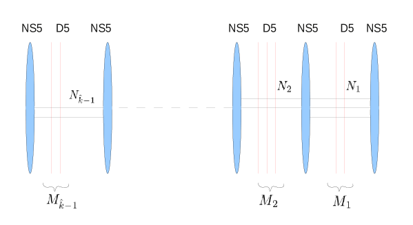
Figure II.3: Brane realization of linear quivers

The brane construction of the linear quivers shown in Figure II.3 is characterized by the following linking numbers

$$l_{i} = j\quad\textrm{for a D5-brane between the $j$-th and $(j+1)$-th NS5 brane}$$ (II.3.22)

$$\hat{l}_{j} = N_{j-1}-N_{j}+\sum_{s=j}^{\hat{k}-1}M_{s}\quad\textrm{for}\quad j=1,..,\hat{k}.\quad(N_{0}=N_{\hat{k}}=0)\,.$$ (II.3.23)

We may move all the NS5-branes to the left and all the D5-branes to the right, noting that a new D3-brane is created every time that a D5 crosses a NS5. In the end, all the D3-branes will be suspended between a NS5-brane on the left and a D5-brane on the right, so that the linking numbers satisfy the sum rule

$$\sum_{i=1}^{k}l_{i}=\sum_{j=1}^{\hat{k}}\hat{l}_{j}\equiv N\,,$$ (II.3.24)

where $N$ is the total number of suspended D3 branes. This implies that the two sets of five-brane linking numbers define two partitions of $N$

$$\rho:\qquad~{}N = l_{1}+\ldots+l_{k}$$ (II.3.25)

$$= \underbrace{1+\ldots+1}_{M_{1}}\,+\,\underbrace{2+\ldots+2}_{M_{2}}\,+\,\ldots+\ldots$$

$$\hat{\rho}:\qquad~{}N = \hat{l}_{1}+\ldots+\hat{l}_{\hat{k}}$$ (II.3.26)

$$= \underbrace{1+\ldots+1}_{\hat{M}_{1}}\,+\,\underbrace{2+\ldots+2}_{\hat{M}_{2}}\,+\,\ldots+\ldots\,.$$

This is the repackaging of the quiver data in terms of partitions of $N$, mentioned above. It is illustrated by Figure II.4.

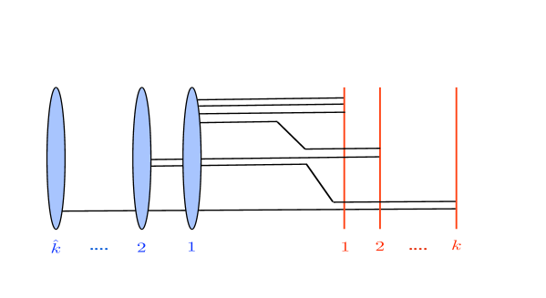
Figure II.4: Pushing all D5-branes to the right of all NS5-branes makes it easy to read the linking numbers, as the net number of D3-branes ending on each five-brane. In this example $\rho=(3,2,\cdots 2)$ and $\hat{\rho}=(4,2,\cdots 1)$.

In the original configuration of Figure II.1 the D5 brane linking numbers are, by construction, positive and non-increasing, i.e. $l_{1}\geq\cdots\geq l_{i}\geq l_{i+1}\cdots\geq l_{k}>0$, but this is not automatic for the linking numbers of the NS5 branes. Requiring that the NS5 brane linking numbers be non-increasing, that is $\hat{l}_{1}\geq\cdots\geq\hat{l}_{i}\geq\hat{l}_{i+1}\cdots\geq\hat{l}_{\hat{k}}=N_{\hat{k}-1}$, is equivalent, as follows from (II.3.23), to

$$M_{i}+N_{i-1}+N_{i+1}\geq 2N_{i}\,.$$ (II.3.27)

This is the same as (II.2.13), the necessary and sufficient conditions for the corresponding (‘good’) quiver gauge theories to flow to an irreducible superconformal field theory in the infrared. Notice that if these conditions are not obeyed the linking numbers of the NS5 branes need not even be positive integers. Furthermore, for the good theories that obey (II.3.27), it follows from the expressions (II.3.23) that the Young tableaux conditions $\rho^{T}>\hat{\rho}$ are automatically satisfied as long as the rank of each gauge-group factor in the quiver diagram is positive.

In the configuration of Figure II.4 on the other hand, the meaning of the above conditions changes. The ordering and positivity of all linking numbers is now automatic (more precisely, it can be trivially arranged by moving 5-branes of the same type past each other). The constraints $\rho^{T}>\hat{\rho}$ on the other hand are non-trivial; they are the ones that guarantee that a supersymmetric configuration like the one of Figure II.1 can be reached by a sequence of Hanany-Witten moves. The two types of configuration shown in the figures are in one-to-one correspondence when all these inequalities are satisfied by the five-brane linking numbers.

Summarizing, the linear-quiver ${\cal N}=4$ gauge theories conjectured in [11] to flow to irreducible fixed points in the infrared (without extra free decoupled multiplets) are labeled in an invariant way by two ordered partitions of $N$, with associated Young tableaux $\rho$ and $\hat{\rho}$ subject to the conditions $\rho^{T}>\hat{\rho}$.

Circular Quivers

The brane configuration corresponding to the circular-quiver gauge theory of Figure II.2 is given in Figure II.5. In this case the $x^{3}$ coordinate along the D3 branes is periodic. Compared to the linear case, there are $N_{\hat{k}}>0$ additional D3 branes extended between the first and the $\hat{k}$th NS5 branes that close the circle. There can be, as well, $M_{\hat{k}}\geq 0$ extra D5 branes giving rise to fundamental hypermultiplets.

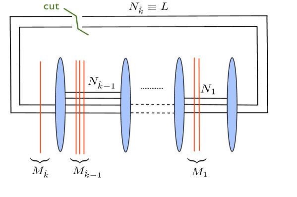
Figure II.5: Brane realization of circular quivers. To attribute linking numbers to the five-branes we cut open the $k$-th stack of D3 branes, and place the $k$-th D5 stack at the left-most end.

We can associate linking numbers to the five-branes by cutting open the circular quiver along one of the suspended D3-brane stacks, say the $k$-th stack. We also choose to place the $\hat{k}$-th stack of D5 branes at the left-most end of the open chain, as shown in Figure II.5. The linking numbers are gauge-variant quantities, and the above choices amount to fixing partially a gauge. In this gauge the linking numbers read:

$$l_{i} = j\quad\textrm{for the $j$-th stack of D5 branes}\,,$$ (II.3.28)

$$\hat{l}_{j} = N_{j-1}-N_{j}+\sum_{s=j}^{\hat{k}}M_{s}\ ,\quad\textrm{with}\quad j=1,..,\hat{k}\ .\quad(N_{0}=N_{\hat{k}})$$ (II.3.29)

As in the case of linear quivers, we label the NS5 branes in order of appearance from right to left, and the D5 branes from left to right.

Defined as above, the linking numbers obey the sum rule (II.3.24) with $N\equiv\sum_{s=1}^{\hat{k}}sM_{s}$. Furthermore the linking numbers of the D5 branes are by construction non-increasing, positive and bounded by the number of NS5 branes, i.e.

$$\hat{k}\geq l_{1}\geq\cdots l_{i}\geq l_{i+1}\cdots\geq l_{k}>0\ .$$ (II.3.30)

What about the linking numbers of NS5 branes? For linear quivers, imposing that the $\hat{l}_{j}$ be non-increasing was equivalent to the Higgsing conditions (IV.4) that singled out the ‘good theories’, i.e. those believed to flow to an irreducible superconformal fixed point in the infrared. Now, the Higgsing conditions can be written as

$$0 \leq N_{j+1}+N_{j-1}-2N_{j}+M_{j}=\hat{l}_{j}-\hat{l}_{j+1}\quad\textrm{for}\,\ j=1,..,\hat{k}-1$$ (II.3.31)

$$0 < N_{1}+N_{\hat{k}-1}-2N_{\hat{k}}+M_{\hat{k}}=\hat{l}_{\hat{k}}-\hat{l}_{1}+\sum_{s=1}^{\hat{k}}M_{s}\,.$$ (II.3.32)

The second line, which gives the condition for Higgsing of the $\hat{k}$-th gauge-group factor, needs explaining. We have assumed that, for this factor, the inequality (IV.4) is strict. A good circular quiver always has at least one such gauge-group factor because, if all the inequalities (IV.4) were saturated, it can be shown that all the $N_{j}$ are equal, and all $M_{j}=0$. So, in this case, there would be only bi-fundamental hypermultiplets, but these cannot break completely the gauge group since they are neutral under the diagonal $U(1)$. This possibility must thus be excluded, i.e. one or more of the inequalities (IV.4) must be strict. We choose to cut open the circular quiver at a D3-brane stack for which $N_{F,j}>2N_{j}$. Without loss of generality this is the $k$-th stack.

The conditions (II.3.31) tell us that the NS5-brane linking numbers are non-increasing. If we want them to be positive, we must impose that

$$\hat{l}_{\hat{k}}=N_{\hat{k}-1}-N_{\hat{k}}+M_{\hat{k}}>0\ .$$ (II.3.33)

If we furthermore want our gauge condition to respect mirror symmetry we must impose the analog of the first inequality (II.3.30), namely

$$\hat{l}_{1}=N_{\hat{k}}-N_{1}+k\leq k\ .$$ (II.3.34)

Together (II.3.33) and (II.3.34) imply (II.3.32), but not the other way around. Fortunately, these conditions can be always satisfied in good quivers, for example by choosing a gauge factor whose rank is locally minimum along the chain (i.e. $N_{\hat{k}}<N_{1},N_{\hat{k}-1}$). With this choice we finally have

$$k\geq\hat{l}_{1}\geq\cdots\hat{l}_{j}\geq\hat{l}_{j+1}\cdots\geq\hat{l}_{\hat{k}}>0\ ,$$ (II.3.35)

so that the NS5-brane and the D5-brane linking numbers are on equal footing. They define two partitions, $\hat{\rho}$ and $\rho$ of the same number $N$.

Contrary to the case of linear quivers, here the partitions do not fully determine the brane configuration. The reason is that the number, $N_{\hat{k}}\equiv L>0$, of D3 branes in the $k$-th stack is still free to vary. We can change it, without changing the linking numbers of the five-branes, by adding or removing D3 branes that wrap the circle (thus increasing or decreasing uniformly all gauge-group ranks). It follows from (II.3.29) that the condition for all gauge-group factors to have positive rank now reads

$$L+\rho^{T}>\hat{\rho}\ \,.$$ (II.3.36)

To understand this constraint intuitively, note that removing $L$ winding D3 branes may convert some stacks of D3 branes to stacks of anti-D3 branes. In the case of linear quivers the inequality $\rho^{T}>\hat{\rho}$ guarantees the absence of anti-D3 branes. Here anti-D3 branes are tolerated, as long as their number is less than $L$.

To any data $(\rho,\hat{\rho},L)$ subject to the constraints (II.3.36), together with the additional conditions $l_{1}\leq\hat{k}$ and $\hat{l}_{1}\leq k$, there corresponds a ‘good’ circular-quiver gauge theory, i.e. one conjectured to flow to an irreducible superconformal theory in the infrared. This description is, however, highly redundant because of the arbitrariness in choosing at which D3-brane stack to cut open the quiver. A generic circular quiver will have many gauge-group factors for which (II.3.33) and (II.3.34) are satisfied, so many different triplets $(\rho,\hat{\rho},L)$ would describe the same SCFT.

To remove this redundancy, one can impose the extra condition that the cut-open segment be of minimal rank globally, i.e. that $L\leq N_{j}$ for all $j$. This condition is compatible with the earlier ones; it amounts to further fixing the gauge. Now removing $L$ winding D3-branes does not create any anti-D3 branes, since $L$ was the absolutely minimal rank. The two partitions thus obey the stronger inequality

$$\rho^{T}\geq\hat{\rho}\ \,.$$ (II.3.37)

As a bonus, the conditions $l_{1}\leq\hat{k}$ and $\hat{l}_{1}\leq k$ are now also automatically satisfied. Note that linear-quiver theories saturating some of the inequalities $\rho^{T}\geq\hat{\rho}$ broke down into smaller decoupled linear quivers plus free hypermultiplets. For circular quivers, on the other hand, these disjoint pieces are reconnected by the $L>0$ winding D3 branes, giving irreducible theories in the infrared.

Summarizing, the circular-quiver gauge theories conjectured to flow to irreducible superconformal field theories in the infrared can be labeled by a positive integer $L$, and by two ordered partitions $\rho$ and $\hat{\rho}$ subject to the condition $\rho^{T}\geq\hat{\rho}$. An alternative but redundant description is in terms of a triplet $(\rho,\hat{\rho},L)$ subject to the looser conditions (II.3.36), together with the additional constraints $l_{1}\leq\hat{k}$ and $\hat{l}_{1}\leq k$. Both descriptions are manifestly mirror-symmetric. As we will later discuss, in the dual supergravity theory these two descriptions correspond to a complete, or to a partial gauge fixing of the 2-form potentials.

II.4 Defect SCFTs

The IR fixed points of the 3d $\mathcal{N}=4$ linear quiver theories described above have a natural extension as defect SCFTs . The theories in question arise as the IR fixed points of $\mathcal{N}=4$ $d=4$ Super-Yang-Mills theory interacting with a 3d linear quiver gauge theory living on a 3d defect. The bulk-boundary couplings are such that half of the bulk supersymmetries are conserved, hence the name of $\frac{1}{2}$-BPS defect SCFTs. Such defect SCFTs with a single 3d hypermultiplet living on the defect and their holography have been considered in [18, 19], where the superconformal action was given . The more general $\frac{1}{2}$-BPS defects have been classified in [14, 20, 11] where they were understood, as in the last subsection, from brane configurations with D3, D5 and NS5 branes.
These general defect SCFTs consist in having a 3d $\mathcal{N}=4$ linear quiver gauge theory living on the defect with supersymmetric couplings to the bulk fields through ”mixed” bifundamental hypermultiplets. To describe the gauge theories we consider it it simpler to start with the brane picture.

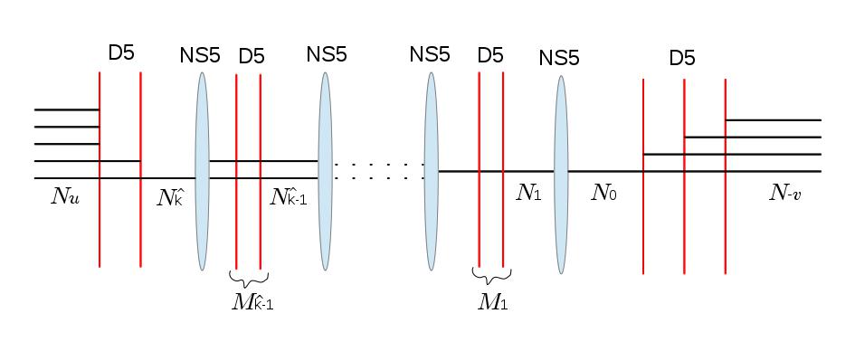
Figure II.6: Brane realization of a defect quiver (flowing to a $\frac{1}{2}$-BPS defect SCFT). The $N_{L}=N_{u}$ ($N_{R}=N_{-v}$) D3-branes on the left (right) are semi infinite in the $x^{3}$ direction.

The brane setup is the same as the one we considered for linear quivers in section II.3 but now we allow for semi-infinite D3-branes ending on the left NS5-brane and semi-infinite D3-branes ending on the right NS5-brane. This is not actually the most general case. We also allow for the semi-infinite D3-branes, say those coming from the left, to end on D5-branes that are placed on the left of the brane configuration, and similarly for the semi-infinite D3-branes coming from the right. A generic brane configuration is given in figure II.6.

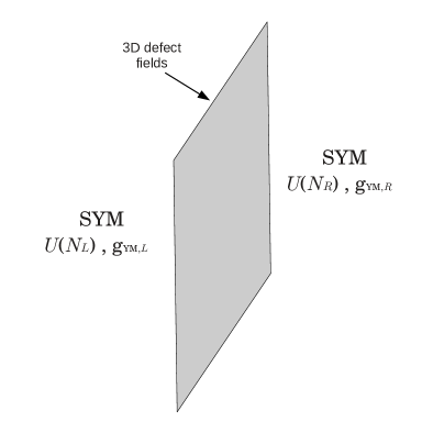
Figure II.7: 4d $\mathcal{N}=4$ SYM with 3-dimensional gauge theory living on a defect. The left and right bulk regions have independent gauge groups and gauge couplings.

Let’s consider the simple cases when there is no extra D5-branes on the left and right of the brane configuration. In this case there are $N_{L}$ semi-infinite D3-branes ending on the left NS5-brane and $N_{R}$ semi-infinite D3-branes ending on the right NS5-brane. The defect gauge theory is easily understood.

The linear quiver theory obtained form the brane configuration when ignoring the semi-infinite D3-branes is the field theory living on the 3-dimensional defect. This defect cuts the 4d space in two regions (see figure II.7), say the left and right regions, and can be seen as a boundary for each of these two half-spaces. On the left region (resp. right region) lives a $\mathcal{N}=4$ $U(N_{L})$ (resp. $U(N_{R})$) SYM theory, with independent gauge couplings $g_{YM}^{L}$ and $g_{YM}^{R}$. To describe the boundary conditions for the bulk fields, focusing on bosonic fields only, one has to decompose the 4d-fields of SYM into $(A_{\mu},X^{1,2,3})$, $\mu=0,1,2$, and $(A^{3},Y^{1,2,3})$, where the $X^{i}$ and $Y^{i}$ are the six scalars. This decomposition corresponds to vector- and hyper-multiplets from a 3d point of view.
Then the bulk fields obey NS5-like boundary conditions on the defect, which means Neumann boundary conditions for $(A_{\mu},X^{1,2,3})$ and Dirichlet boundary conditions for $(A^{3},Y^{1,2,3})$ (see [14]) . The defect fields are coupled to the bulk fields of the left region through an additional defect hypermultiplet transforming in the fundamental of the left node $U(N_{\hat{k}-1})$ of the quiver and in the fundamental of the boundary $U(N_{L})$, which means a 3d $\mathcal{N}=4$ coupling to the 3d multiplet $(A^{\mu}_{L},X^{1,2,3}_{L})$ induced on the boundary. The coupling to the 4d fields of the right region is similar : NS5-like boundary conditions for the right bulk fields and another ”mixed” defect hypermultiplet transforming in the fundamental of the right node $U(N_{1})$ of the quiver and in the fundamental of the boundary $U(N_{R})$. The theory content is summarized by the quiver diagram of II.8 where the end-nodes correspond to the left and right 4d $\mathcal{N}=4$ SYM with their respective gauge groups $U(N_{L})$ and $U(N_{R})$, and the links from these nodes to the linear quiver nodes correspond to the additional ”mixed bulk-defect“ bifundamental hypermultiplets.

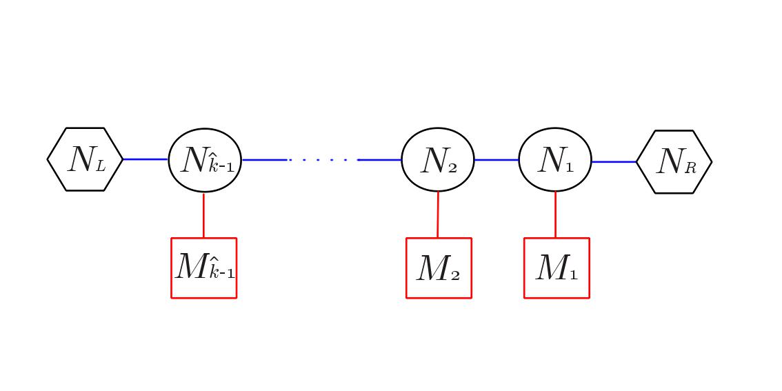
Figure II.8: Quiver picture of a 3d defect field theory with NS5-like boundary conditions for the bulk fields (without extra D5-branes) . The meaning of each element is the same as for a 3d linear quiver except for the two external nodes (hexagons) corresponding to $U(N_{L})$ and $U(N_{R})$ 4d $\mathcal{N}=4$ vector multiplets (SYM) on the two half spaces and the blue line connecting them to the 3d quiver corresponding to the mixed ”bulk-defect“ bifundamental 3d hypermultiplets.

The more general brane configuration when semi-infinite D3-branes end on D5-branes placed at the left or on the right of all the NS5-branes correspond to having more general $\frac{1}{2}$-BPS boundary conditions for the bulk fields. These general boundary conditions are described in detail in [14] and we will only recall here their main features. They break the gauge symmetry $U(N_{L})$ (resp. $U(N_{R})$) to a smaller $U(N_{\hat{k}})$ (resp. $U(N_{0})$) on the defect and involve mixed NS5-like and D5-like boundary conditions for the bulk fields. The general boundary conditions are given by Nahm’s equation, which allow pole singularities on the boundary for the scalar fields (Nahm poles). The solutions to Nahm’s equations depend on the linking numbers of the external D5-branes, that define an embedding of $su(2)$ into $su(N_{L})$ ($su(N_{R})$), and additional moduli that should be taken to zero in our context, to preserve conformal symmetry (this is the same as being at the origin of the Higgs branch in a sense).

The presence of these additional D5-branes change the boundary conditions for the bulk fields but not the matter content of the field theory living on the defect, except in the case of an external D5-branes without D3-brane ending on it. Such a D5-brane corresponds to a defect hypermultiplet transforming in the fundamental representation of the boundary $U(N_{0})$ (or $U(N_{\hat{k}})$).

The general $\frac{1}{2}$-BPS defect SCFTs can be summarized in the quiver picture of figure II.9. Compared to II.8 there are extra nodes on the left and on the right, corresponding to the numbers of D3-branes in the segments between the external adjacent D5-branes, accounting for the left and right boundary conditions.

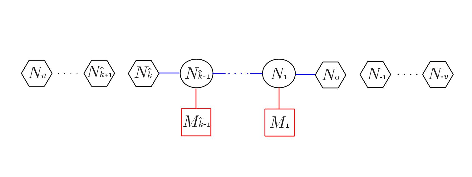
Figure II.9: Quiver picture of a general $\frac{1}{2}$-BPS 3d-defect field theory. The hexagonal nodes denote the number of D3-branes in the segments inbetween the external D5-branes,encoding to the boundary conditions for the bulk fields ([14]) with $N_{u}=N_{L}$ and $N_{-v}=N_{R}$.

From figure II.6 we can associate a linking number to each 5-brane with the same definition II.3.21 as for linear quivers, defining two non-standard partitions $\rho,\hat{\rho}$. We call them ”non-standard“ because there may be negative linking numbers both for the D5 and NS5-branes.

As in the case of linear quivers, the conditions of irreducibility of the IR SCFT are given by the ordering of the linking numbers in non-decreasing order from left to right for NS5-brane and from right to left for the D5-branes. The ordering of the NS5-brane linking numbers is again equivalent to the Gaiotto-Witten conditions IV.4. The ordering of D5-brane linking number was automatic for linear quivers but it is not the case here because of the additional left and right D5-branes. Ordering the linking numbers of the D5-branes amounts to say that the number of (semi-infinite) D3-branes ending on the left-most D5-brane is bigger than the number of D3-branes ending on the second left-most D5-brane, … etc, and similarly for the right-most D5-branes. According to [11] it ensures again that there is no decoupling hypermultiplets in the infrared limit.

Moving the NS5-branes on the left and the D5-branes on the right, it is easy to see that $\rho$ defines now an ordered partition of $N-N_{R}$, while $\hat{\rho}$ defines now an ordered partition of $N-N_{L}$, with $N$ the total number of D3-branes inbetween the D5 and NS5-branes. The partitions may contain negative numbers.

To summarize, the defect quivers are given by the data $(\rho,\hat{\rho},N_{L},N_{R},g_{YM}^{(L)},g_{YM}^{(R)})$, where $g_{YM}^{(L)}$ and $g_{YM}^{(R)}$ are the Yang-Mills couplings of SYM on the left and right half-spaces. As for linear quivers, this data obeys the sumrule

$$\sum_{i=1}^{k}l_{i}+N_{R}=\sum_{j=1}^{\hat{k}}\hat{l}_{j}+N_{L}\quad.$$ (II.4.38)

We can denote $\mathcal{D}(\rho,\hat{\rho},N_{L},N_{R},g_{YM}^{(L)},g_{YM}^{(R)})$ the corresponding infrared fixed point SCFT.

As for linear and circular quivers the partitions $\rho$ and $\hat{\rho}$ have to satisfy some inequalities, so that they define a defect quiver with positive ranks. The positivity of the ranks translate in this case into the inequalities

$$N_{0}+\rho^{T}_{>0}>\hat{\rho}\quad,\quad N_{0}>0\ ,$$ (II.4.39)

where $\rho^{T}_{>0}$ is the transposed Young tableau of the partition $\rho$ truncated to its positive components .
Note that the condition $N_{0}>0$ (resp. $N_{\hat{k}}>0$) ensures $N_{i}>0$ for $i<0$ (resp. $N_{i}>0$ for $i>\hat{k}$) because of the ordering of the linking numbers.

When $N_{R}=N_{0}$ (no D5-branes on the right of the quiver) these inequalities reduce to

$$N_{R}+\rho^{T}>\hat{\rho}\quad,\quad N_{R}>0\ .$$ (II.4.40)

The saturation of one inequality corresponds again to having a node with zero rank. The defect SCFT then breaks into two independant boundary SCFTs, which are defect SCFTs with $N_{L}=0$ or $N_{R}=0$ : SYM theory on a half-space coupled to a 3d boundary fields.

II.5 Partition function of deformed linear quivers

In this section we review the proposal of [23] for the explicit analytic expression for the linear quivers $T^{\rho}_{\hat{\rho}}(SU(N))$ deformed by real masses $m_{j}$ and Fayet-Iliopoulos parameters $\eta_{j}\equiv\xi_{j}-\xi_{j+1}$ on the 3-sphere. This explicit expression was derived from the matrix models obtained by the techniques of localization (see section II.1 above) and make mirror symmetry manifest. The matrix models do not depend on the Yang-Mills coupling $g_{YM}$, which means that it computes directly the partition function in the infrared limit $g_{YM}\rightarrow+\infty$. We will use it in chapter IV when we compute free energies at the superconformal point (zero mass and FI terms).

To express the analytic expression for the partition function we need to introduce what we call the deformed partitions and the deformation $N$-vectors.

To each 5-brane in the brane picture we have associated a linking number $l_{i}$ or $\hat{l}_{j}$. We can associate also to each 5-brane a deformation parameter which corresponds to its position in transverse space.
The D5-branes can be displaced along $(x_{7},x_{8},x_{9})$ (without breaking additional supersymmetries) giving three mass parameters (real and complex masses) to the corresponding fundamental hypermultiplet. The masses transform as a triplet of the $SU(2)_{R}\simeq SO(3)$ rotation group of $(x_{7},x_{8},x_{9})$ and two of them can be set to zero (see §II.1). So we associate only one deformation parameter $m_{i}$ to each D5-branes and it corresponds to giving a real mass $m_{i}$ to the fundamental hypermultiplets.
Similarly the NS5-branes can be displaced along $(x_{4},x_{5},x_{6})$ (without breaking additional supersymmetries), giving three real parameters that transform as a triplet of the $SU(2)_{L}\simeq SO(3)$ rotation group of $(x_{4},x_{5},x_{6})$. Again two of them are set to zero by using this rotation symmetry. The non-vanishing parameters $\xi_{j}$ are associated to the NS5-branes (one for each) and they are related to the Fayet-Iliopoulos parameters $\eta_{j}$ of the gauge nodes as $\eta_{j}=\xi_{j+1}-\xi_{j}$. To summarize we have one linking number and one real deformation parameter for each 5-brane.

We define the deformed partitions, that we call again $\rho$ and $\hat{\rho}$, as

$$\rho :=\Big{(}(l_{1},m_{1}),(l_{2},m_{2}),\ ...\ ,(l_{k},m_{k})\Big{)}$$

$$\hat{\rho} :=\Big{(}(\hat{l}_{1},\xi_{1}),(\hat{l}_{2},\xi_{2}),\ ...\ ,(\hat{l}_{\hat{k}},\xi_{\hat{k}})\Big{)}$$ (II.5.41)

and the deformation $N$-vectors

$$\vec{m} :=\big{(}\ \textrm{coord}(\vec{m}_{1})\ ,\ \textrm{coord}(\vec{m}_{2})\ ,\ ...\ ,\ \textrm{coord}(\vec{m}_{k})\ \big{)}$$

$$\textrm{with}\quad\vec{m}_{j}=\left\{\ m_{j}+i\Big{(}\frac{l_{j}+1}{2}-1\Big{)},\ m_{j}+i\Big{(}\frac{l_{j}+1}{2}-2\Big{)},\ ...\ ,\ m_{j}+i\Big{(}\frac{l_{j}+1}{2}-l_{j}\Big{)}\ \right\}$$

$$\vec{\xi} :=\big{(}\ \textrm{coord}(\vec{\xi}_{1})\ ,\ \textrm{coord}(\vec{\xi}_{2})\ ,\ ...\ ,\ \textrm{coord}(\vec{\xi}_{\hat{k}})\ \big{)}$$ (II.5.42)

$$\textrm{with}\quad\vec{\xi}_{j}=\bigg{\{}\ \xi_{j}+i\Big{(}\frac{\hat{l}_{j}+1}{2}-1\Big{)},\ \xi_{j}+i\Big{(}\frac{\hat{l}_{j}+1}{2}-2\Big{)},\ ...\ ,\ \xi_{j}+i\Big{(}\frac{\hat{l}_{j}+1}{2}-\hat{l}_{j}\Big{)}\ \bigg{\}}\ ,$$

where coord$(\vec{v})=v_{1},v_{2},v_{3},...,v_{p}$ for a vector $\vec{v}$ with $p$ coordinates.
Note that $\vec{m}$ and $\vec{\xi}$ are vectors with $N$ coordinates, while $\vec{m}_{j}$ and $\vec{\xi}_{j}$ are vectors with $l_{j}$, resp. $\hat{l}_{j}$, coordinates.

For instance for the linear quiver in figure II.10, we have

$$\rho =\Big{(}(2,m_{1}),(1,m_{2}),(1,m_{3}),(1,m_{4})\Big{)}$$

$$\hat{\rho} =\Big{(}(2,\xi_{1}),(2,\xi_{2}),(1,\xi_{3})\Big{)}$$

$$\vec{m} =\left(m_{1}+\frac{i}{2}\ ,\ m_{1}-\frac{i}{2}\ ,\ m_{2}\ ,\ m_{3}\ ,\ m_{4}\right)$$ (II.5.43)

$$\vec{\xi} =\left(\xi_{1}+\frac{i}{2}\ ,\ \xi_{1}-\frac{i}{2}\ ,\ \xi_{2}+\frac{i}{2}\ ,\ \xi_{2}-\frac{i}{2}\ ,\ \xi_{3}\right)\ .$$

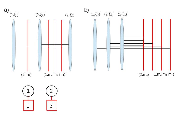
Figure II.10: a) Brane configuration and quiver for the theory $T^{(2111)}_{(221)}(SU(5))$. b) Brane configuration with separated NS5-branes and D5-branes. Below each 5-brane is indicated the linking number and deformation parameter associated to it.

The conjecture of [23] is that the partition function for the deformed $T^{\rho}_{\hat{\rho}}(SU(N))$ is given up to a phase by

$$Z=\frac{\mathcal{Z}}{\Delta_{\hat{\rho}}(\vec{\xi})\Delta_{\rho}(\vec{m})}\quad,\quad\mathcal{Z}=\sum_{w\in\mathfrak{S}^{N}}(-1)^{w}\ e^{2i\pi\,\vec{\xi}.w(\vec{m})}$$ (II.5.44)

with $\mathfrak{S}^{N}$ the group of permutations of $N$ elements, $(-1)^{w}$ the signature of a permutation $w$ and $\vec{\xi}.w(\vec{m})=\sum_{j=1}^{N}\xi_{j}m_{w(j)}$. The definition of the determinants $\Delta_{\hat{\rho}}(\vec{\xi})$ and $\Delta_{\rho}(\vec{m})$ requires to arrange the deformation $N$-vectors $\vec{\xi}$ and $\vec{m}$ as tableaux $[\xi]=([\xi]_{ab})$ and $[m]=([m]_{ab})$ whose lines are the vectors $\vec{\xi}_{1},\vec{\xi}_{2},...,\vec{\xi}_{\hat{k}}$, resp. $\vec{m}_{1},\vec{m}_{2},...,\vec{m}_{k}$ and we have

$$\Delta_{\hat{\rho}}(\vec{\xi}) =\prod_{b=1}^{\hat{l}_{\hat{k}}}\prod_{a<a^{\prime}}\textrm{sh}([\xi]_{ab}-[\xi]_{a^{\prime}b})$$

$$\Delta_{\rho}(\vec{m}) =\prod_{b=1}^{l_{k}}\prod_{a<a^{\prime}}\textrm{sh}([m]_{ab}-[m]_{a^{\prime}b})\ .$$ (II.5.45)

For instance for II.5 we have

$$[\xi] =\begin{bmatrix}\xi_{1}+\frac{i}{2}&\xi_{1}-\frac{i}{2}\\ \xi_{2}+\frac{i}{2}&\xi_{2}-\frac{i}{2}\\ \xi_{3}&.\end{bmatrix}\quad,\quad[m]=\begin{bmatrix}m_{1}+\frac{i}{2}&m_{1}-\frac{i}{2}\\ m_{2}&.\\ m_{3}&.\\ m_{4}&.\end{bmatrix}$$ (II.5.46)

where a square with ”.“ is not a box of the tableau (these tableaux have five boxes each), in particular it does not produce a sh-factors in II.5.
And the determinant are

$$\Delta_{\hat{\rho}}(\vec{\xi}) =-\ \textrm{ch}(\xi_{1}-\xi_{2})\ \textrm{ch}(\xi_{1}-\xi_{3})\ \textrm{sh}(\xi_{2}-\xi_{3})^{2}$$ (II.5.47)

$$\Delta_{\rho}(\vec{m}) =-i\ \textrm{sh}(m_{1}-m_{2})\ \textrm{sh}(m_{2}-m_{3})\ \textrm{sh}(m_{1}-m_{3})\ \textrm{ch}(m_{1}-m_{4})\ \textrm{ch}(m_{2}-m_{4})\ \textrm{ch}(m_{3}-m_{4})\ .$$

Let’s make a few comments about this formula.

First, the partition function (II.5.44) is manifestly invariant under the simultaneous exchange of the deformed partitions $\rho$ and $\hat{\rho}$ (exchange of the partitions and of the parameters $m$ and $\xi$).This is a manifestation of the 3d mirror symmetry.

Second, (II.5.44) vanishes unless $\rho^{T}\geq\hat{\rho}$ [23]. This is consistent with the condition (II.2.14) for the existence of a non-trivial IR SCFT.

Third, the expression (II.5.44) is mysteriously complexe and moreover has a (parameter-independent) phase ambiguity. We will concentrate (in chapter IV) on the absolute value of the $S^{3}$ partition function and define the free energy as $F=-\log|Z|$.

$T(SU(N))$ gauge theory :

The simplest linear quiver theory one can study turns out to be the so-called $T(SU(N))$ SCFT and its deformed version. The linear quiver is given by the two partitions

$$\rho=\hat{\rho}=\big{[}\overbrace{1,1,...,1}^{N}\big{]}\ .$$ (II.5.48)

The gauge group is $U(1)\times U(2)\times...\times U(N-1)$ and the matter content, on top of the bifundamental hypermultiplets consists of $N$ hypermultiplets transforming in the fundamental representation of the $U(N-1)$ node. The quiver and the brane configuration are presented in figure II.11. Strictly speaking $T(SU(N))$ is the IR fixed point SCFT of the linear quiver.
The theory has a group of global symmetry $SU(N)_{F}\times SU(N)_{J}$ with $SU(N)_{F}$ acting on the $N$ fundamental hypermultiplets (which transform again in the fundamental representation) and the $SU(N)_{J}$ arising as an enhancement of the topological $U(1)^{N-1}$ symmetry at the IR fixed point. $T(SU(N))$ is known to be invariant under mirror symmetry, which exchanges the two $SU(N)$ global symmetries. This is the larger group of global symmetries accessible for a $T^{\rho}_{\hat{\rho}}(SU(N))$ linear quiver.

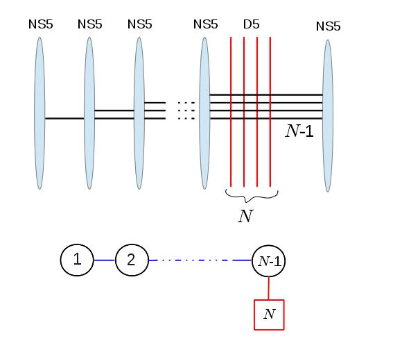
Figure II.11: Brane configuration and quiver of the $T(SU(N))$ theory.

The theory has deformation parameters which can be thought as vev for scalars in background $U(1)$ vector multiplets (meaning vector coupling to $U(1)$ global symmetry current). These parameters are $N$ masses $m_{j}$ for $N$ fundamental hypermultiplets and $N-1$ FI parameters $\eta_{j}$ for the $N-1$ nodes. These FI parameters are conveniently recast in $N$ parameters $\xi_{j}$ defined by $\eta_{j}=\xi_{j}-\xi_{j+1}$ as explained above.

The deformed partitions for $T(SU(N))$ are

$$\rho :=\Big{(}(1,m_{1}),(1,m_{2}),\ ...\ ,(1,m_{N})\Big{)}$$

$$\hat{\rho} :=\Big{(}(1,\xi_{1}),(1,\xi_{2}),\ ...\ ,(1,\xi_{N})\Big{)}\ ,$$ (II.5.49)

and the deformation $N$-vectors and the determinants are simply

$$\vec{m} =(m_{1}\ ,\ m_{2},\ ...\ ,\ m_{N})$$

$$\vec{\xi} =(\xi_{1}\ ,\ \xi_{2},\ ...\ ,\ \xi_{N})$$

$$\Delta_{\rho}(\vec{m}) =\prod_{i<j}^{N}\textrm{sh}(m_{i}-m_{j})$$ (II.5.50)

$$\Delta_{\hat{\rho}}(\vec{\xi}) =\prod_{i<j}^{N}\textrm{sh}(\xi_{i}-\xi_{j})$$

The matrix model giving the partition function was computed in [32, 23] and turned out to be one of the simplest non-abelian partition function.

$$Z^{T(SU(N))} =(-i)^{\frac{N(N-1)}{2}}e^{-2i\pi\xi_{N}\sum_{j}^{N}m_{j}}\frac{\sum_{w\in\mathfrak{S}_{N}}(-1)^{w}\,e^{2i\pi\sum_{j}^{N}\xi_{j}m_{w(j)}}}{\prod_{j<k}^{N}\textrm{sh}(\xi_{j}-\xi_{k})\textrm{sh}(m_{j}-m_{k})}$$ (II.5.51)

with $\mathfrak{S}^{N}$ the group of permutations of $N$ elements. This reproduces, up to a phase, the prediction of II.5.44.

As will be shown in chapter IV, the $T(SU(N))$ SCFT plays a distinguished role among the $T^{\rho}_{\hat{\rho}}(SU(N))$ theories as the SCFT with maximal free energy.

Chapter III Supergravity solutions and the correspondence

In this chapter we present the large class of type IIB supergravity solutions with $OSp(4|4)$ symmetry that we constructed. We expose our AdS/CFT dictionnary with all “irreducible” infrared super-conformal fixed points of $d=3$, $\mathcal{N}=4$ linear quivers, circular quivers and $d=4$ SYM $\frac{1}{2}$-BPS defect theories. We emphasize the relation with the rich brane picture. Interesting limiting geometries are also discussed.

III.1 History of the type IIB supergravity solution with $OSp(4|4)$ symmetry

The IIB supergravity solutions that we study in this presentation have a local structure that was derived by D’Hoker, Estes and Gutperle in [21, 22]. These solutions have been searched as gravity duals of $\frac{1}{2}$-BPS 3d-defect SCFTs or infinitely thin BPS domain walls in 4d $\mathcal{N}=4$ super-Yang-Mills theory (described in section II.4). Before the explicit solutions were derived, [76] already classified these $\frac{1}{2}$-BPS defect SCFTs and the corresponding supergravity solutions, that are domain walls interpolating between two $AdS_{5}\times S^{5}$ asymptotic regions. In [76] the domain wall solutions were already described as $AdS_{4}\times S^{2}\times S^{2}\ltimes\Sigma_{2}$ warped geometries where $\Sigma_{2}$ is a strip with D5-brane singularities on one boundary and NS5-brane singularities on the other boundary. The data describing the solutions was predicted to be encoded in the fluxes escaping the singularities. This is exactly the features of the solutions we describe in this chapter, realizing the geometric transitions between branes and fluxes. Other type IIB gemetries dual to $\frac{1}{2}$-BPS operators in $\mathcal{N}=4$ SYM were found previously ([77, 78, 79, 80]). Preliminary work studying the $\frac{1}{2}$-BPS $AdS_{4}$ embedding of probe D5-branes into $AdS_{5}\times S^{5}$ can be found in [81, 82].

The strategy of [21] to derive the relevant solutions is to encode the $SO(2,3)\times SO(3)\times SO(3)$ bosonic symmetries of $OSp(4|4)$ in the ansatz

$$ds^{2}=f_{4}^{2}(z,\bar{z})\,ds^{2}_{AdS_{4}}+f_{1}^{2}(z,\bar{z})\,ds^{2}_{S^{2}_{(1)}}+f_{2}^{2}(z,\bar{z})\,ds^{2}_{S^{2}_{(2)}}+4\rho(z,\bar{z})^{2}\,dzd\bar{z}\ .$$ (III.1.1)

with $f_{4},f_{1},f_{2},\rho$ real functions of $z,\bar{z}$, and to look for solutions with 16 supersymmetries (8 Poincaré + 8 super-conformal), the 16 independent supersymmetry generators being Killing spinors of $AdS_{4}\times S^{2}_{(1)}\times S^{2}_{(2)}$. The BPS equations provide first order diferential equations. The solutions are found to be expressed in terms of two real harmonic functions $h_{1},h_{2}$ on $\Sigma$, describing the cases of vanishing axion field. The solutions with non-vanishing axion are obtained by $SL(2,\mathbb{R})$ transformations that are symmetries of type IIB supergravity.

In [22] the authors exposed the conditions for the regularity of the solutions, putting severe constraints on the harmonic functions $h_{1},h_{2}$. An important constraint is that on the boundary of $\Sigma$ one harmonic function and the normal derivative of the other should vanish, so that the boundary is partitioned in segments where $h_{1}=\partial_{\bot}h_{2}=0$ or $h_{2}=\partial_{\bot}h_{1}=0$. A consequence of this condition is that one 2-sphere or the other vanishes at each point of the boundary and, combining with the normal direction, has the local topology of a 3-sphere. Thus the boundary points of $\Sigma$ are actually interior points of the geometry. The regularity conditions allow for very specific kinds of point singularities on the boundary of $\Sigma$ that we detail below.

In [8], we showed that the asymptotic $AdS_{5}\times S^{5}$ regions can be removed from the geometry by taking the limit of zero asymptotic radius, without destroying the solutions. The resulting geometries are dual to the IR fixed point of 3d $\mathcal{N}=4$ linear quiver that have the same $OSp(4|4)$ symmetries.

III.2 Solutions of IIB supergravity : the case of the strip

We will now exhibit the solutions of type-IIB supergravity that are holographic duals of superconformal field theories discussed above (chapter II).

First we review the general local solutions of type IIB supergravity that have the appropriate $OSp(4|4)$ superconformal symmetries found in [21, 22]. Then we present the solutions on the strip that are related to the (IR fixed point of) linear quivers of section II.2 and to the defect SCFT of section II.4. We show how the ”closure” of the asymptotic regions leads to the supergravity solutions that will be dual to the linear quivers. The solutions we present also contain, in some limit, the supergravity backgrounds dual to 4-dimensional $\mathcal{N}=4$ SYM with a 3-dimensional boundary CFT [83].

III.2.1 Local solutions

References [21, 22] give the general local solutions of type-IIB supergravity preserving the superconformal symmetry $OSp(4|4)$. This group is the supergroup of the 3d $\mathcal{N}=4$ SCFTs. The solutions are parameterized by a choice of a 2-dimensional Riemann surface $\Sigma$ with boundary and by two real harmonic functions on $\Sigma$, $h_{1}$ and $h_{2}$. We then define auxiliary functions on $\Sigma$

$$W=\partial\bar{\partial}(h_{1}h_{2})\ ,\qquad N_{j}=2h_{1}h_{2}|\partial h_{j}|^{2}-h_{j}^{2}W,$$ (III.2.2)

with $\partial\equiv\partial_{z}$ , $\bar{\partial}\equiv\partial_{\bar{z}}$, the complex $z$ parametrizing $\Sigma$.
In terms of these auxiliary functions the metric in Einstein frame can be written as

$$ds^{2}=f_{4}^{2}ds^{2}_{AdS_{4}}+f_{1}^{2}ds^{2}_{S^{2}_{1}}+f_{2}^{2}ds^{2}_{S^{2}_{2}}+4\rho^{2}dzd\bar{z}\ ,$$ (III.2.3)

where the warp factors are given by

$$f_{4}^{8}=16\frac{N_{1}N_{2}}{W^{2}}\ ,\ \ \ f_{1}^{8}=16h_{1}^{8}\frac{N_{2}W^{2}}{N_{1}^{3}}\ ,\ \ \ f_{2}^{8}=16h_{2}^{8}\frac{N_{1}W^{2}}{N_{2}^{3}}\ ,\ \ \ \rho^{8}=\frac{N_{1}N_{2}W^{2}}{h_{1}^{4}h_{2}^{4}}\ .$$ (III.2.4)

This geometry is supported by non-vanishing “matter” fields, which include the (in general complex) dilaton-axion field

$$S=\chi+ie^{2\phi}=i\sqrt{N_{2}\over N_{1}}\ ,$$ (III.2.5)

in addition to 3-form and 5-form backgrounds. To specify the corresponding gauge potentials one needs the dual harmonic functions, defined by

$$h_{1}=-i({\cal A}_{1}-\bar{\cal A}_{1})\qquad \rightarrow\qquad h_{1}^{D}={\cal A}_{1}+\bar{\cal A}_{1}\ ,$$ (III.2.6)

$$h_{2}={\cal A}_{2}+\bar{\cal A}_{2}\qquad \rightarrow\qquad h_{2}^{D}=i({\cal A}_{2}-\bar{\cal A}_{2})\ .$$ (III.2.7)

The constant ambiguity in the definition of the dual functions is related to changes of the background fields under large gauge transformations. The NS-NS and R-R three forms can be written as

$$H_{(3)}=\omega^{\,45}\wedge db_{1}\qquad{\rm and}\qquad F_{(3)}=\omega^{\,67}\wedge db_{2}\ ,$$ (III.2.8)

where $\omega^{\,45}$ and $\omega^{\,67}$ are the volume forms of the unit-radius spheres ${\rm S}_{1}^{2}$ and ${\rm S}_{2}^{2}$, while

$$b_{1} =2ih_{1}{h_{1}h_{2}(\partial h_{1}\bar{\partial}h_{2}-\bar{\partial}h_{1}\partial h_{2})\over N_{1}}+2h_{2}^{D}\ ,$$ (III.2.9)

$$b_{2} =2ih_{2}{h_{1}h_{2}(\partial h_{1}\bar{\partial}h_{2}-\bar{\partial}h_{1}\partial h_{2})\over N_{2}}-2h_{1}^{D}\ .$$ (III.2.10)

The expression for the gauge-invariant self-dual 5-form is a little more involved:

$$F_{(5)}=-4\,f_{4}^{\,4}\,\omega^{\,0123}\wedge{\cal F}+4\,f_{1}^{\,2}f_{2}^{\,2}\,\omega^{\,45}\wedge\omega^{\,67}\wedge(*_{2}{\cal F})\ ,$$ (III.2.11)

where $\omega^{\,0123}$ is the volume form of the unit-radius ${\rm AdS}_{4}$, ${\cal F}$ is a 1-form on $\Sigma$ with the property that $f_{4}^{\,4}{\cal F}$ is closed, and $*_{2}$ denotes Poincaré duality with respect to the $\Sigma$ metric. The explicit expression for ${\cal F}$ is given by

$$f_{4}^{\,4}{\cal F}=dj_{1}\ \qquad{\rm with}\qquad j_{1}=3{\cal C}+3\bar{\cal C}-3{\cal D}+i\frac{h_{1}h_{2}}{W}\,(\partial h_{1}\bar{\partial}h_{2}-\bar{\partial}h_{1}\partial h_{2})\ ,$$ (III.2.12)

where ${\cal C}$ and ${\cal D}$ are defined by $\partial{\cal C}={\cal A}_{1}\partial{\cal A}_{2}-{\cal A}_{2}\partial{\cal A}_{1}$ and ${\cal D}=\bar{\cal A}_{1}{\cal A}_{2}+{\cal A}_{1}\bar{\cal A}_{2}$.

For any choice of $h_{1}$ and $h_{2}$, equations (III.2.2) to (III.2.12) give local solutions of the supergravity equations which are invariant under $OSp(4|4)$. Global consistency puts severe constraints on these harmonic functions and on the surface $\Sigma$. There is no complete classification of all consistent choices for this data.

What has been shown [21, 22] is that the most general type-IIB solution with the $OSp(4|4)$ symmetry can be brought to the above form by an $SL(2,\mathbb{R})$ transformation. This acts as follows on the dilaton-axion and 3-form fields:

$$S\to{aS+b\over cS+d}\ ,\qquad\left(\begin{array}[]{c}H_{(3)}\\ F_{(3)}\end{array}\right)\to\left(\begin{array}[]{cc}d&-c\\ -b&a\end{array}\right)\left(\begin{array}[]{c}H_{(3)}\\ F_{(3)}\end{array}\right)\ .$$ (III.2.19)

The Einstein-frame metric and the 5-form $F_{(5)}$ are left unchanged.

III.2.2 Admissible singularities

The holomorphic functions ${\cal A}_{1}$ and ${\cal A}_{2}$ are analytic in the interior of $\Sigma$, but can have singularities on its boundary. Refs. [21, 22] identified three kinds of “admissible” singularities, i.e. singularities that can be interpreted as brane sources in string theory. Two of these are logarithmic-cut singularities and correspond to the two elementary kinds of five-brane. In local coordinates, in which the boundary of $\Sigma$ is the real axis, these singularities read

$$\underline{\rm D5}:\qquad{\cal A}_{1}=-i\gamma\,{\rm log}w+\cdots\ ,\qquad{\cal A}_{2}=-ic+\cdots\ ,$$ (III.2.20)

$$\underline{\rm NS5}:\qquad{\cal A}_{1}=-\hat{c}+\cdots\ ,\qquad{\cal A}_{2}=-\hat{\gamma}\,{\rm log}w+\cdots\ .$$ (III.2.21)

Here $\gamma,\hat{\gamma},c,\hat{c}$ are real parameters related to the brane charges, and the dots denote subleading terms, which are analytic at $w=0$ and have the same reality properties on the boundary as the leading terms. These reality properties imply that, in the case of the D5-brane, $h_{1}$ and $h_{2}$ obey respectively Neumann and Dirichlet boundary conditions, i.e. $(\partial-\bar{\partial})h_{1}=h_{2}=0$ on the boundary of $\Sigma$. For the NS5 brane the roles of the two harmonic functions are exchanged.

The vanishing of the harmonic function $h_{j}$ implies that the corresponding 2-sphere $S_{j}^{\,2}$ shrinks to a point. This ensures that the points on the boundary of $\Sigma$, away from the singularities, correspond to regular interior points of the ten-dimensional geometry. Non-contractible cycles, which support non-zero brane charges, are obtained by the fibration of one or both 2-spheres over any curve that (semi)circles the singularity on $\partial\Sigma$. For instance in the case of the NS5-brane $I\times S_{1}^{\,2}$, with $I$ the interval shown in figure III.1, is topologically a non-contractible 3-sphere. The appropriately normalized flux of $H_{(3)}$ through this cycle is the number of NS5-branes:

$$\hat{N}_{5}\,=\,{1\over 4\pi^{2}\alpha^{\prime}}\int_{I\times S_{1}^{\,2}}H_{(3)}={2\over\pi\alpha^{\prime}}h_{2}^{D}\Bigl{|}_{\partial I}\qquad\Longrightarrow\ \ \hat{N}_{5}\,=\ {4\over\alpha^{\prime}}\,\hat{\gamma}\ .$$ (III.2.22)

In evaluating the flux we have taken $I$ to be infinitesimally small, and we used the fact that in the expression (III.2.9) only $h_{2}^{D}$ is discontinuous across the singularity on the real axis. We also assumed that the logarithmic cut lies outside the surface $\Sigma$, so that fields in the interior of $\Sigma$ are all continuous (see figure III.1).

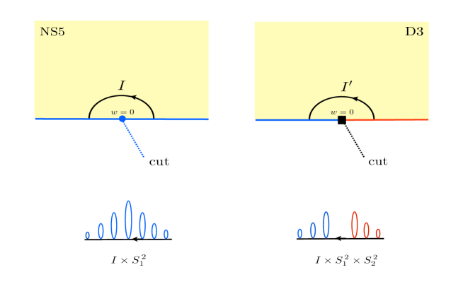
Figure III.1: Local singularities corresponding to a NS5-brane (left) and a D3-brane (right), as explained in the text. The boundary of $\Sigma$ is colored red or blue according to which of the two 2-spheres, $S_{1}^{\,2}$ or $S_{2}^{\,2}$, shrinks at this part of the boundary to zero. The non-contractible cycles supporting the brane charges are $I\times S_{1}^{\,2}$, $I\times S_{1}^{\,2}\times S_{2}^{\,2}$ and $I^{\prime}\times S_{1}^{\,2}\times S_{2}^{\,2}$, with $I$ and $I^{\prime}$ the (oriented) solid semicircles of the figure. These cycles are topologically equivalent to a 3-sphere, a 3-sphere times a 2-sphere, and a 5-sphere. The broken lines indicate the logarithmic (on the left) and square root (on the right) branch cuts.

In addition to 5-brane charge, the singularities (III.2.21) also carry D3-brane charge. The corresponding flux threads the 5-cycle $I\times S_{1}^{\,2}\times S_{2}^{\,2}$, which is topologically the product of a 3-sphere with a 2-sphere. There is a well-known subtlety in the definition of this charge, because of the Chern-Simons term in the IIB supergravity action [8, 84, 85]. In the case at hand the conserved flux is the integral of the gauge-variant 5-form $F_{(5)}^{\prime}=F_{(5)}+C_{(2)}\wedge H_{(3)}$, which obeys a non-anomalous Bianchi identity $dF_{(5)}^{\prime}=0$ in a region without brane sources. Further details about the conservation of 5-form flux and the choice of relevant 5-form to integrate will be detailed below when we consider the annulus case (to avoid redundancy). The number of D3-branes inside the NS5-brane stack is thus given by

$$\hat{N}_{3}\,=\,{1\over(4\pi^{2}\alpha^{\prime})^{2}}\int_{I\times S_{1}^{\,2}\times S_{2}^{\,2}}[F_{(5)}+C_{(2)}\wedge H_{(3)}]\,=\,-{2\over\pi\alpha^{\prime}}\,\hat{N}_{5}\,h_{1}^{D}\Bigl{|}_{w=0}\ .$$ (III.2.23)

It can be checked, by taking again $I$ arbitrarily small, that $F_{(5)}$, as well as all terms in the expression for $C_{(2)}$ other than $h_{1}^{D}$, do not contribute to the above flux. This explains the second equality, leading finally to

$$\hat{N}_{3}\,=\ \left({4\over\alpha^{\prime}}\right)^{2}\,\left({\hat{\gamma}\,\hat{c}\over\pi}\right)\ .$$ (III.2.24)

Note that $\hat{N}_{3}$ depends on the potential $C_{(2)}$ at the position of the 5-brane singularity, and may change under large gauge transformations. This is related to the Hanany-Witten effect [12], an issue to which we will return in the next subsection.

In principle, using $SL(2,\mathbb{R})$ transformations one can convert the NS5-brane solution to a more general $(p,q)$ fivebrane solution. Such transformations generate, however, a non-trivial Ramond-Ramond axion background, so $(p,q)$ fivebranes cannot coexist with the NS5-brane in the IIB solutions described above for which the axion vanishes. The $(p,q)$-5-branes will reappear later when we consider the action of $SL(2,\mathbb{R})$ transformations on the solutions we are presently studying. There is one exception to the rule: the S-duality transformation converts the NS5-brane to a D5-brane without generating an axion background. Combined with an exchange of the two 2-spheres, S-duality acts as follows on the harmonic functions:

$$\left(\begin{array}[]{c}i{\cal A}_{2}\\ -{\cal A}_{1}\end{array}\right)\ \xrightarrow{S}\ \left(\begin{array}[]{c}{\cal A}_{1}\\ i{\cal A}_{2}\end{array}\right)\ .$$ (III.2.29)

This gives the D5-brane singularity anticipated already in equation (III.2.21). The integer D5-brane and D3-brane charges read

$$N_{5}={4\over\alpha^{\prime}}\,\gamma\,,\qquad N_{3}\,=\ \left({4\over\alpha^{\prime}}\right)^{2}\,\left({\gamma\,c\over\pi}\right)\ .$$ (III.2.30)

Note that the D3-brane charge is here the flux of the 5-form $F_{(5)}-B_{(2)}\wedge F_{(3)}$, which is the S-duality transform of $F_{(5)}+C_{(2)}\wedge H_{(3)}$. This gauge-variant form is well-defined in any patch around the D5-brane singularity as long as this patch does not contain NS5-brane sources.

The last kind of singularity, which can coexist with D5- and NS5-brane singularities, is the one describing free D3-branes, with no associated fivebrane charge. In this case the holomorphic functions have square-root rather than logarithmic cuts [22]

$$\underline{\rm D3}:\qquad{\cal A}_{1}={1\over\sqrt{w}}(a_{1}+b_{1}w+\cdots)\ ,\qquad{\cal A}_{2}={1\over\sqrt{w}}(a_{2}+b_{2}w+\cdots)\ .$$ (III.2.31)

Such singularities change the boundary condition of $h_{1}$ from Neumann to Dirichlet, and the boundary condition of $h_{2}$ from Dirichlet to Neumann. This is illustrated in the right part of figure III.1. The integer D3-brane charge is given by

$$n_{3}\,=\,{1\over\left(4\pi^{2}\alpha^{\prime}\right)^{2}}\int_{I^{\prime}\times S_{1}^{\,2}\times S_{2}^{\,2}}F_{(5)}\ =\ \left({4\over\alpha^{\prime}}\right)^{2}\,\,{(a_{1}b_{2}-a_{2}b_{1})\over 2\pi}\ .$$ (III.2.32)

The ten-dimensional geometry near the D3-brane singularity is an $AdS_{5}\times S^{5}$ throat with radius $L$ given by $L^{4}=4\pi\alpha^{\prime\,2}|n_{3}|$.

III.2.3 Linear-quiver geometries and AdS/CFT dictionary

Consider two harmonic functions with the singularity structure shown in figure III.2. The corresponding geometries have the field-theory interpretation of superconformal domain walls in ${\cal N}=4,D=4$ Super Yang Mills [11], breaking $SU(2,2|4)$ to $OSp(4|4)$. If $n_{3}^{\pm}$ are the D3-brane charges of the two boundary-changing (black-box) singularities, then the domain wall separates two gauge theories with gauge groups $U(n_{3}^{-})$ and $U(n_{3}^{+})$. One may decouple the three-dimensional SCFT that lives on the domain wall from the bulk four-dimensional Yang-Mills theories by setting $a_{j}^{\pm}=0$. Equation (III.2.31) shows that in this case $n_{3}^{+}=n_{3}^{-}=0$. The square-root singularities of the harmonic functions are then simply coordinate singularities, while the infinite $AdS_{5}\times S^{5}$ throats are replaced by regular interior points in ten-dimensions.

In [83] another limit of these harmonic functions was taken, namely the limit in which only one $AdS_{5}\times S^{5}$ region is capped off $n^{+}_{3}=0$. The geometries then correspond to coupling $\mathcal{N}=4$ D=4 Super-Yang-Mills to a 3-dimensional boundary CFT.

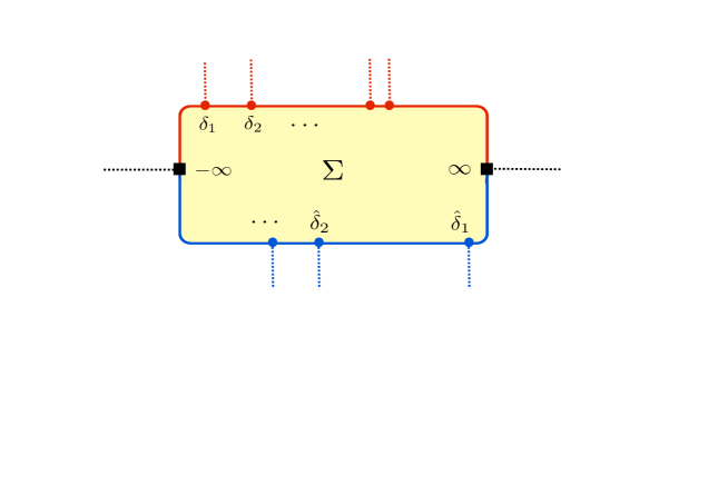
Figure III.2: Structure of singularities of the harmonic functions for the linear-quiver geometries. The two boundary-changing singularities at $\pm\infty$, corresponding to $AdS_{5}\times S^{5}$ throats, can be capped off by choosing $a_{1}=a_{2}=0$, as described in the text. They become regular interior points of the ten-dimensional geometry.

Following references [37, 8], we choose $\Sigma$ to be the infinite strip parametrized by a complex $z=x+iy$ , $x\in(-\infty,+\infty)$ , $y\in[0,\frac{\pi}{2}]$, and the harmonic functions to be given by

$${\cal A}_{1} =\alpha\sinh(z-\beta)\ -i\sum_{a=1}^{p}\gamma_{a}\ln\,\tanh\left({\small{\frac{i\pi}{4}-\frac{z-\delta_{a}}{2}}}\right)\ ,$$

$${\cal A}_{2} =\hat{\alpha}\cosh(z-\hat{\beta})\ -\sum_{b=1}^{\hat{p}}\hat{\gamma}_{b}\ln\tanh\left(\frac{z-\hat{\delta}_{b}}{2}\right)\ .$$ (III.2.33)

The parameters ($\alpha,\beta,\gamma_{a},\delta_{a}$) and ($\hat{\alpha},\hat{\beta},\hat{\gamma}_{b},\hat{\delta}_{b}$) are all real. The only other condition on this set of parameters, explained in [22], is that $\alpha,\gamma_{1},\cdots,\gamma_{p}$ must be all positive or all negative and similarly for $\hat{\alpha},\hat{\gamma}_{1},\cdots,\hat{\gamma}_{\hat{p}}$. If not, the solution has curvature singularities supported on a one-dimensional curve in the interior of $\Sigma$, which have no interpretation in string theory.
Here $\delta_{1}<\delta_{2}<...<\delta_{p}$ are the positions of the D5-brane singularities on the upper boundary of the strip, whereas $\hat{\delta}_{1}>\hat{\delta}_{2}>...>\hat{\delta}_{\hat{p}}$ are the positions of the NS5-brane singularities on the lower boundary. It can be checked that on these two boundaries $h_{1}$ obeys, respectively, Neumann and Dirichlet conditions, while $h_{2}$ has Dirichlet and Neumann conditions.

Here we focus on the solutions with $n_{3}^{+}=n_{3}^{-}=0$ when the two asymptotic $AdS_{5}\times S^{5}$ regions at $\pm\infty$ are capped off. This correspond to taking $\alpha=\hat{\alpha}=0$ and the solutions are simply given by

$${\cal A}_{1} =-i\sum_{a=1}^{p}\gamma_{a}\ln\,\tanh\left({\small{\frac{i\pi}{4}-\frac{z-\delta_{a}}{2}}}\right)\quad,\quad{\cal A}_{2} =-\sum_{b=1}^{\hat{p}}\hat{\gamma}_{b}\ln\tanh\left(\frac{z-\hat{\delta}_{b}}{2}\right)\ .$$ (III.2.34)

The boundary-changing square-root singularities are at $z=\pm\infty$. In the local coordinate $w=e^{\mp z}$ one can verify easily that $a_{j}^{\pm}=0$, so these points at infinity correspond to regular interior points of the ten-dimensional geometry.

To simplify the formulae we will adopt from now on the (non-standard) convention $\alpha^{\prime}=4$. Equations (III.2.30) and (III.2.22) give the numbers of NS5-branes and D5-branes for each fivebrane singularity:

$$N_{5}^{(a)}=\gamma_{a}\ ,\qquad\hat{N}_{5}^{(b)}=\hat{\gamma}_{b}\ .$$ (III.2.35)

Unbroken supersymmetry requires that there are only branes (or only anti-branes) of each kind. Thus all the $\gamma_{a}$ must have the same sign, and likewise for all the $\hat{\gamma}_{b}$. This agrees with the regularity condition mentioned above . We choose to take all $\gamma_{a}>0$ and all $\hat{\gamma}_{b}>0$. The other possibilities are obtained by charge conjugations and do not lead to different CFT duals. Dirac quantization forces furthermore these parameters to be integer.

Next let us consider the D3-brane charge. Inserting the harmonic functions (III.2.34) inside the expressions (III.2.30) and (III.2.24) gives

$$N_{3}^{(a)}=N_{5}^{(a)}\sum_{b=1}^{\hat{p}}\hat{N}_{5}^{(b)}\,{2\over\pi}{\rm arctan}(e^{\hat{\delta}_{b}-\delta_{a}})\ ,$$

$$\hat{N}_{3}^{(b)}=-\hat{N}_{5}^{(b)}\sum_{a=1}^{p}N_{5}^{(a)}\,{2\over\pi}{\rm arctan}(e^{\hat{\delta}_{b}-\delta_{a}})\ ,$$ (III.2.36)

where we used the identity $i\,$log tanh$({i\pi\over 4}-{x\over 2})=-$2 arctan($e^{x}$). As already noted in the previous subsection, this calculation of the D3-brane charge depends on the 2-form potentials $B_{(2)}$ and $C_{(2)}$ and is, a priori, ambiguous. One may indeed add a real constant to ${\cal A}_{1}$, or an imaginary constant to ${\cal A}_{2}$, thereby changing $h_{j}^{D}$ without affecting $h_{j}$. This gauge ambiguity is also reflected in the arbitrary choice of Riemann sheet for the logarithmic functions that enter in equations (III.2.34).

We fix this ambiguity by placing all logarithmic cuts outside $\Sigma$, as in figure III.2, and by choosing the sheet so that the imaginary part of (${\rm ln\,tanh}\,z$) vanishes when $z$ goes to $+\infty$ on the real axis. This implies that the arctangent functions take values in the interval $[0,\pi/2]$. Our choice of gauge is continuous in the interior of $\Sigma$ (which is covered by a single patch), and sets $B_{(2)}=0$ at $+\infty$ and $C_{(2)}=0$ at $-\infty$. With this choice, D5-branes at $\delta=+\infty$ and NS5-branes at $\hat{\delta}=-\infty$ do not contribute to the D3-brane charge. Placing, on the other hand, one NS5-brane at $\hat{\delta}=+\infty$ adds one unit of D3-brane charge to each D5-brane, while placing one D5-brane at $\delta=-\infty$ adds one unit of charge to each NS5-brane. This can be understood as a holographic manifestation of the Hanany-Witten effect.

Since this story will be important to us later, let us explain it a little more. The 2-form potential $B_{(2)}$ is proportional to the volume form ($\omega^{45}$) of the sphere $S_{1}^{\,2}$, which shrinks to a point in the lower boundary of the strip (the blue line in figure III.2). The solution III.2.34 is such that $B_{(2)}$ is constant on the lower boundary intervals between the NS5-singularities and jumps accross each singularity proportionally to the NS5-flux it supports. When $B_{(2)}\not=0$ on a boundary interval, this interval corresponds to a Dirac singularity of codimension 3 in (the 9-dimensional) space. This is unobservable if

$${1\over 2\pi\alpha^{\prime}}\int_{S_{1}^{\,2}}B_{(2)}\in 2\pi\mathbb{Z}\ \Longrightarrow\ B_{(2)}\Bigl{|}_{{\rm Im}z=0}\ =\ \pi\alpha^{\prime}\omega^{45}\times({\rm integer})\ .$$ (III.2.37)

With our choice of gauge,

$$B_{(2)}\Bigl{|}_{{\rm Im}z=0}\ =\ \pi\alpha^{\prime}\omega^{45}\times\sum_{b=1}^{\beta}\hat{N}_{5}^{(b)}\qquad{\rm for}\ \ \ \hat{\delta}_{\beta+1}<{\rm Re}z<\hat{\delta}_{\beta}\ .$$ (III.2.38)

Large gauge transformations change $B_{(2)}$ everywhere in the strip by a multiple of $\pi\alpha^{\prime}\omega^{45}$, and can remove the Dirac sheet in one of the intervals of the boundary. For us this was the interval $(\hat{\delta}_{1},\infty)$. A similar story holds also for the upper (red) boundary and the 2-form $C_{(2)}$. The D3-brane charges with our choice of gauge agree with the invariant linking numbers defined in chapter II section II.3.

The brane engineering of the dual gauge field theories [12, 11] involves $N$ D3-branes suspended between $\hat{k}$ NS5-branes on the left and $k$ D5-branes on the right. In the IIB supergravity the corresponding numbers are:

$$N=\sum_{a=1}^{p}N_{3}^{(a)}=-\sum_{b=1}^{\hat{p}}\hat{N}_{3}^{(b)}\ ,\qquad k=\sum_{a=1}^{p}N_{5}^{(a)}\ ,\qquad\hat{k}=\sum_{b=1}^{\hat{p}}\hat{N}_{5}^{(b)}\ .$$ (III.2.39)

The way in which the D3-branes are suspended to the five-branes is given by two partitions $\rho$ and $\hat{\rho}$, which define the linear-quiver gauge theory and its IR fixed point $T^{\rho}_{\hat{\rho}}(SU(N))$. These partitions are given in terms of the linking numbers:

$$\rho =\Big{(}\overbrace{l^{(1)},l^{(1)},..,l^{(1)}}^{N_{5}^{(1)}},\ \overbrace{l^{(2)},l^{(2)},..,l^{(2)}}^{N_{5}^{(2)}},\ ...\ ,\ \overbrace{l^{(p)},l^{(p)},..,l^{(p)}}^{N_{5}^{(p)}}\Big{)}\ ,$$

$$\hat{\rho} =\Big{(}\overbrace{\hat{l}^{(1)},\hat{l}^{(1)},..,\hat{l}^{(1)}}^{\hat{N}_{5}^{(1)}},\ \overbrace{\hat{l}^{(2)},\hat{l}^{(2)},..,\hat{l}^{(2)}}^{\hat{N}_{5}^{(2)}},\ ...\ ,\ \overbrace{\hat{l}^{(\hat{p})},\hat{l}^{(\hat{p})},..,\hat{l}^{(\hat{p})}}^{\hat{N}_{5}^{(\hat{p})}}\Big{)}\ ,$$ (III.2.40)

where

$$l^{(a)}=\frac{N_{3}^{(a)}}{N_{5}^{(a)}}\quad,\quad\hat{l}^{(b)}=-\frac{\hat{N}_{3}^{(b)}}{\hat{N}_{5}^{(b)}}\ .$$ (III.2.41)

Here $l^{(a)}$ is the number of D3-branes ending on each D5-brane in the $a$th stack, while $\hat{l}^{(b)}$ is the number of D3-branes emanating from each NS5-brane in the $b$th stack. Because these numbers must be integers, the parameters $\delta_{a}$ and $\hat{\delta}_{b}$ are quantized. In all one has $2p+2\hat{p}-1$ parameters, since a global translation of all the $\delta_{a}$ and $\hat{\delta}_{b}$ does not change the solution. The parameters of the quiver are $N_{5}^{(a)},l^{(a)},\hat{N}_{5}^{(b)},\hat{l}^{(b)}$ subject to one constraint (III.2.39), which expresses the conservation of D3-brane charge. The two parameter counts therefore match.

The linking numbers of the supergravity solutions obey the inequalities $\rho^{T}>\hat{\rho}$, which were the conditions for the existence of an infrared fixed point of the quiver gauge theory [11], see II.3. On the supergravity side, the inequalities follow from the fact that $0<{\rm arctan}(x)<\pi/2$ for positive $x$. The details of the computations are presented in appendix B. This is a non-trivial check of the AdS/CFT correspondence.

III.2.4 Defect SCFT solutions

To complete the discussion on supergravity solutions on the strip, let’s mention more general solutions III.2.3 with arbitrary $\alpha,\beta,\hat{\alpha},\hat{\beta}$. These geometries have already been studied in [37] in the contect of the search for graviton zero mode localized on the strip.
In this case the internal geometry is non-compact and we have two asymptotic $AdS_{5}\times S^{5}$ regions at $x=\pm\infty$. These solutions are believed to be dual to $D=4$ $\mathcal{N}=4$ Super-Yang-Mills coupled to a $\frac{1}{2}$-BPS 3-dimensional defect CFT [18] describe in section II.4. The defect splits the 4d space in two regions with independent gauge groups $U(N_{-})$ and $U(N_{+})$ and Yang-Mills gauge couplings $g_{-}$ and $g_{+}$ that correspond to the two asymptotic $AdS_{5}\times S^{5}$ regions, as in the original Maldacena setup (see section I.1).

The asymptotics of the solutions III.2.3 when $x\rightarrow\pm\infty$ are given by the $AdS_{5}\times S^{5}$ supergravity solution with different radii $L_{\pm}$ and dilaton values $e^{2\phi_{\pm}}$.

$$ds^{2} =L_{\pm}^{2}\left(dx^{2}+\cosh^{2}(x)\,ds^{2}_{AdS_{4}}+dy^{2}+\sin^{2}(y)\,ds^{2}_{S_{1}^{2}}+\cos^{2}(y)\,ds^{2}_{S_{2}^{2}}\right)$$

$$F^{5} =-4L_{\pm}^{4}(1+\star)\omega^{4567y}\ ,$$ (III.2.42)

where $\omega^{4567y}$ is the volume form of the unit 5-sphere. In terms of the supergravity parameters, the asymptotic data reads

$$L_{\pm}^{4} =16\,\left(\alpha\hat{\alpha}\,\cosh(\beta-\hat{\beta})+\sum_{a=1}^{p}2\hat{\alpha}\gamma_{a}\,e^{\pm(\delta_{a}-\hat{\beta})}+\sum_{b=1}^{\hat{p}}2\alpha\hat{\gamma}_{b}\,e^{\pm(\hat{\delta}_{b}-\beta)}\right)$$

$$e^{2\phi_{\pm}} =\frac{\hat{\alpha}\,e^{\pm\hat{\beta}}+\sum_{b=1}^{\hat{p}}4\hat{\gamma}_{b}\,e^{\pm\hat{\delta}_{b}}}{\alpha\,e^{\pm\beta}+\sum_{a=1}^{p}4\gamma_{a}\,e^{\pm\delta_{a}}}\ .$$ (III.2.43)

the relations to the gauge theory data are the usual

$$L_{\pm}^{4} =4\pi|N_{\pm}|\alpha^{\prime 2}$$

$$e^{2\phi_{\pm}} =g_{\pm}\ .$$

The 5-brane charges are the same as for the linear quiver geometries ($\alpha^{\prime}=4$)

$$N_{5}^{(a)}=\gamma_{a}\ ,\qquad\hat{N}_{5}^{(b)}=\hat{\gamma}_{b}\ .$$ (III.2.44)

The (quantized) D3-brane charges follow from the general formulas III.2.23, III.2.24, III.2.30, and are given in the usual gauge $C_{2}=0$ on the upper boundary segment $(-\infty,\delta_{1}]$, $B_{2}=0$ on the lower boundary segment $[\hat{\delta}_{1},+\infty)$ by

$$N_{3}^{(a)}=\frac{2}{\pi}\,N_{5}^{(a)}\left(-\frac{\hat{\alpha}}{2}\sinh(\delta_{a}-\hat{\beta})+\sum_{b=1}^{\hat{p}}\hat{N}_{5}^{(b)}\,\textrm{arctan}(e^{\hat{\delta}_{b}-\delta_{a}})\right)\ ,$$

$$\hat{N}_{3}^{(b)}=-\frac{2}{\pi}\,\hat{N}_{5}^{(b)}\left(\frac{\alpha}{2}\sinh(\hat{\delta}_{b}-\beta)+\sum_{a=1}^{p}N_{5}^{(a)}\,\textrm{arctan}(e^{\hat{\delta}_{b}-\delta_{a}})\right)\ .$$ (III.2.45)

The asymptotic (quantized) D3-charges $N_{\pm}$ measured with approriate orientation are

$$N_{\pm} =\pm\frac{1}{4\pi}\,\left(\alpha\hat{\alpha}\,\cosh(\beta-\hat{\beta})+\sum_{a=1}^{p}2\hat{\alpha}\,N_{5}^{(a)}\,e^{\pm(\delta_{a}-\hat{\beta})}+\sum_{b=1}^{\hat{p}}2\alpha\,\hat{N}_{5}^{(b)}\,e^{\pm(\hat{\delta}_{b}-\beta)}\right)\ .$$ (III.2.46)

One can check that the D3-charge is conserved in the geometry

$$N_{+}+N_{-}+\sum_{a=1}^{p}N_{5}^{(a)}+\sum_{b=1}^{\hat{p}}\hat{N}_{5}^{(b)}=0\ .$$ (III.2.47)

The $2(p+\hat{p})+3$ parameters of the supergravity solution III.2.3 are now recast in terms of the data $(N_{+},N_{-},N_{5}^{(a)},\hat{N}_{5}^{(b)},g_{+},g_{-})$ which obey III.2.47.

The relation to the $\frac{1}{2}$-BPS defect SCFTs described in section II.4 is very close to what we had in the case of linear quivers. The two partitions $\rho$ and $\hat{\rho}$ are again defined by

$$\rho =\Big{(}\overbrace{l^{(1)},l^{(1)},..,l^{(1)}}^{N_{5}^{(1)}},\ \overbrace{l^{(2)},l^{(2)},..,l^{(2)}}^{N_{5}^{(2)}},\ ...\ ,\ \overbrace{l^{(p)},l^{(p)},..,l^{(p)}}^{N_{5}^{(p)}}\Big{)}\ ,$$

$$\hat{\rho} =\Big{(}\overbrace{\hat{l}^{(1)},\hat{l}^{(1)},..,\hat{l}^{(1)}}^{\hat{N}_{5}^{(1)}},\ \overbrace{\hat{l}^{(2)},\hat{l}^{(2)},..,\hat{l}^{(2)}}^{\hat{N}_{5}^{(2)}},\ ...\ ,\ \overbrace{\hat{l}^{(\hat{p})},\hat{l}^{(\hat{p})},..,\hat{l}^{(\hat{p})}}^{\hat{N}_{5}^{(\hat{p})}}\Big{)}\ ,$$ (III.2.48)

where

$$l^{(a)}=\frac{N_{3}^{(a)}}{N_{5}^{(a)}}\quad,\quad\hat{l}^{(b)}=-\frac{\hat{N}_{3}^{(b)}}{\hat{N}_{5}^{(b)}}\ .$$ (III.2.49)

And the bulk SYM data are simply related to the asymptotic data of the supergravity solution

$$N_{L} =-N_{-}\quad,\quad g_{YM}^{(L)\ 2}=g_{-}\ ,$$

$$N_{R} =N_{+}\qquad,\quad g_{YM}^{(R)\ 2}=g_{+}\ .$$ (III.2.50)

The corresponding $\frac{1}{2}$-BPS defect SCFT is then $\mathcal{D}(\rho,\hat{\rho},-N_{-},N_{+},g_{-}^{1/2},g_{+}^{1/2})$.

Note the $l^{(a)}$ and $\hat{l}^{(b)}$ may be negative as the linking numbers of the gauge theory description and that $\sum_{a=1}^{p}l^{(a)}N_{5}^{(a)}=N-N_{R}$ and $\sum_{b=1}^{\hat{p}}\hat{l}^{(b)}\hat{N}_{5}^{(b)}=N-N_{L}$ with

$$N =\frac{1}{4\pi}\,\Big{(}\alpha\hat{\alpha}\,\cosh(\beta-\hat{\beta})+\sum_{a=1}^{p}2\hat{\alpha}\,N_{5}^{(a)}\,e^{-\delta_{a}+\hat{\beta}}+\sum_{b=1}^{\hat{p}}2\alpha\,\hat{N}_{5}^{(b)}\,e^{\hat{\delta}_{b}-\beta}$$

$$\hskip 56.9055pt+\ 8\sum_{a=1}^{p}\sum_{b=1}^{\hat{p}}\hat{N}_{5}^{(a)}N_{5}^{(b)}\,\textrm{arctan}(e^{\hat{\delta}_{b}-\delta_{a}})\Big{)}\ ,$$ (III.2.51)

consistently with the fact that $\rho$ is a partition of $N-N_{R}$, while $\hat{\rho}$ is a partition of $N-N_{L}$.

The two partitions have to satisfy the inequalities II.4.39 which ensures that no anti-D3-branes will appear in the brane picture corresponding to the defect SCFT. The cases of negative linking number for D5-branes make the inequalities difficult to express on the supergravity side, so we have only checked them for solutions with only positive D5-linking numbers. In this case the inequalities takes the simpler form II.4.40 and the explicit computations of appendix B can be easily adapted to the case of the domain wall solutions, using the explicit formula for the charges III.2.45, III.2.46, to show that the inequalities II.4.40 are satisfied (it comes down to the trivial inequalities $2\sinh(x)<e^{x}$ and $\frac{2}{\pi}\arctan(e^{x})<1$).

All the formulas for the linear quiver geometries are obtained by setting $\alpha=\hat{\alpha}=0$, corresponding to $N_{\pm}=0$.

III.3 Circular quiver geometries : from strip to annulus

We present now how the geometries on the strip lead under periodic identification to the supergravity solutions where $\Sigma$ is an annulus and we show how to relate them to the SCFTs arising from the flow of the circular quivers presented in chapter II.

A class of three-dimensional ${\cal N}=4$ superconformal field theories that arise from circular quivers are known to admit an M-theory description in terms of orbifolds of the seven-sphere [86, 87, 30]. By taking a certain (large $L$) smearing limit of our solutions, T-dualizing the periodic coordinate of the annulus and lifting the resulting type-IIA background to eleven dimensions, we reproduce the relevant M-theory geometries ${\rm AdS}_{4}\times{\rm S}^{7}/(\mathbb{Z}_{k}\times\mathbb{Z}_{\hat{k}})$. In the process one looses however the dependence on the full quiver data $(\rho,\hat{\rho},L)$. This data can be in principle encoded in the non-contractible 3-cycles of the compact space and the associated 3-form fluxes [30, 88, 89, 90]. The 3-cycles degenerate however in the orbifold limit and we are not aware of any solutions of eleven-dimensional supergravity that resolve the singularity on the M-theory side. By contrast in our IIB solutions, the full data is encoded in the positions of five-brane throats along the annulus circle.

III.3.1 Solutions on the annulus

The strategy for constructing holographic IIB duals for the circular quivers is the following: one starts from the linear-quiver solutions that we have just described, and arranges the five-branes in infinite pedrodic arrays along the $x$ axis. The holomorphic functions ${\cal A}_{j}$ become logarithms of quasi-periodic elliptic functions. Modding out by discrete translations corresponding to the period of the array then converts the strip domain, $\Sigma$, to an annulus, and the dual linear-quiver theories to theories based on circular quivers.

More explicitly, given a set of fivebrane singularities at $\delta_{a}$ and $\hat{\delta}_{b}$, we may always pick a positive parameter $t$ such that, after a rigid translation, $0\leq\delta_{a}\leq 2t$ and $0\leq\hat{\delta}_{b}\leq 2t$. Replicating the fivebrane sources with periodicity $2t$ then leads to the following harmonic functions

$$h_{1} =-\sum_{a=1}^{p}\gamma_{a}\ln\bigg{[}\prod_{n=-\infty}^{\infty}\tanh\bigg{(}\frac{i\pi}{4}-\frac{z-(\delta_{a}+2nt)}{2}\bigg{)}\bigg{]}+c.c.\ ,$$ (III.3.52)

$$h_{2} =-\sum_{b=1}^{\hat{p}}\hat{\gamma}_{b}\ln\bigg{[}\prod_{n=-\infty}^{\infty}\tanh\bigg{(}\frac{z-(\hat{\delta}_{b}+2nt)}{2}\bigg{)}\bigg{]}+c.c.\ .$$ (III.3.53)

These functions are manifestly periodic under translations by $2t$, so we are free to identify $z\equiv z+2t$ thereby converting the strip $\Sigma$ to an annulus. Figure III.3 depicts this annular domain in the $w$-plane, where $w={\rm exp}({i\pi z/t})$.

Figure III.3: The annulus $\Sigma$ for the type-IIB solutions that are dual to $D=3,{\cal N}=4$ circular-quiver theories. $\Sigma$ is the infinite strip in the $z$ plane modulo the translations $z\to z+2t$ (left), or the annular domain in the $w={\rm exp}(i\pi z/t)$ plane (right). The radius of the inner boundary of the annulus is $\tilde{q}^{1/2}$ where $\tilde{q}={\rm exp}(-\pi^{2}/t)$ is the exponentiated dual modulus of the elliptic $\vartheta$-functions. The monodromies of $h_{j}^{D}$ around the curve $C$ give the total number of NS5 and D5-branes, as explained in the main text.

To see that the infinite products in the above expressions converge, we will rewrite them in terms of elliptic $\vartheta$-functions (we use the conventions of reference [Green:1987mn]). This can be done with the help of the identity

$$\Bigl{|}\frac{\vartheta_{1}(\nu|\tau)}{\vartheta_{2}(\nu|\tau)}\Bigr{|}\,=\,\left|\prod_{n=-\infty}^{\infty}\tanh(i\pi\nu+nt)\,\right|\ ,\qquad{\rm where}\quad e^{i\pi\tau}=e^{-t}\ .$$ (III.3.54)

The proof of this identity follows from the product formulae for the $\vartheta$-functions

$$\vartheta_{1}(\nu|\tau)=2e^{i\pi\tau/4}\sin(\pi\nu)\prod_{n=1}^{\infty}(1-e^{2ni\pi\tau})(1-e^{2ni\pi\tau}e^{2\pi i\nu})(1-e^{2ni\pi\tau}e^{-2\pi i\nu})\ ,$$ (III.3.55)

$$\vartheta_{2}(\nu|\tau)=2e^{i\pi\tau/4}\cos(\pi\nu)\prod_{n=1}^{\infty}(1-e^{2ni\pi\tau})(1+e^{2ni\pi\tau}e^{2\pi i\nu})(1+e^{2ni\pi\tau}e^{-2\pi i\nu})\ .$$ (III.3.56)

Note that the modular parameter is $\tau=it/\pi$, because the hyperbolic tangents are periodic under $z\to z+2\pi i$. Inserting the identity (III.3.54) in (III.3.52) leads to the following expressions for $h_{1}$ and $h_{2}$:

$$h_{1} =-\sum_{a=1}^{p}\gamma_{a}\ln\bigg{[}\frac{\vartheta_{1}\left(\nu_{a}|\tau\right)}{\vartheta_{2}\left(\nu_{a}|\tau\right)}\bigg{]}+c.c.\ ,\ \qquad{\rm with}\ \ \ i\,\nu_{a}=-\frac{z-\delta_{a}}{2\pi}+\frac{i}{4}\ ,$$ (III.3.57)

$$h_{2} =-\sum_{b=1}^{\hat{p}}\hat{\gamma}_{b}\ln\bigg{[}\frac{\vartheta_{1}\left(\hat{\nu}_{b}|\tau\right)}{\vartheta_{2}\left(\hat{\nu}_{b}|\tau\right)}\bigg{]}+c.c.\ ,\ \ \qquad{\rm with}\ \ \ i\,\hat{\nu}_{b}=\frac{z-\hat{\delta}_{b}}{2\pi}\ .$$ (III.3.58)

These harmonic functions are well-defined everywhere inside the annulus. They have logarithmic singularities on the boundaries, wherever $\nu_{a}$ or $\hat{\nu}_{b}$ vanish.

Decomposing $h_{j}$ into holomorphic and anti-holomorphic parts requires, as in the previous subsection, a choice of gauge. A convenient choice is to make the ${\cal A}_{j}$ analytic in the interior of the covering strip, before the periodic identification of $z$. This amounts to placing again all logarithmic branch cuts outside the strip. With this understanding, and recalling that the Jacobi $\vartheta$-functions are holomorphic, we have

$${\cal A}_{1}=-i\sum_{a=1}^{p}\gamma_{a}\ln\bigg{(}\frac{\vartheta_{1}\left(\nu_{a}|\tau\right)}{\vartheta_{2}\left(\nu_{a}|\tau\right)}\bigg{)}+\varphi_{1}\ ,\ \qquad{\cal A}_{2}=-\sum_{b=1}^{\hat{p}}\hat{\gamma}_{b}\ln\bigg{(}\frac{\vartheta_{1}\left(\hat{\nu}_{b}|\tau\right)}{\vartheta_{2}\left(\hat{\nu}_{b}|\tau\right)}\bigg{)}+i\varphi_{2}\ ,$$ (III.3.59)

where the constant phases $\varphi_{1}$ and $\varphi_{2}$ are residual quantized gauge degrees of freedom, corresponding to large gauge transformations of the 2-form potentials. As in the case of the linear quiver, we may use this residual freedom to enforce the absence of Dirac singularities in one interval on each annulus boundary.

Unlike $h_{j}$, the above holomorphic functions and the dual harmonic functions $h_{j}^{D}$ are not periodic under $z\to z+2t$. Their gauge-invariant holonomies (or Wilson lines) give the total fivebrane charges. To see why, note that translating $z\to z+2t$ changes all the arguments $\nu_{a}$ by $it/\pi$ (and all the $\hat{\nu}_{b}$ by $-it/\pi$). From the product formulae (III.3.55) one finds that under these translations the $\vartheta$-functions are quasi-periodic:

$$\vartheta_{1}(\nu+{it\over\pi}|\tau)=-e^{-2\pi i\nu+t}\vartheta_{1}(\nu|\tau)\ ,\qquad\vartheta_{2}(\nu+{it\over\pi}|\tau)=e^{-2\pi i\nu+t}\vartheta_{2}(\nu|\tau)\ .$$ (III.3.60)

The ratio $\vartheta_{1}/\vartheta_{2}$ changes only by a minus sign. Thus ln($\vartheta_{1}/\vartheta_{2})\to$ln($\vartheta_{1}/\vartheta_{2})\mp i\pi$ when $\nu\to\nu\pm it/\pi$, from which we conclude

$${\cal A}_{1}(z+2t)={\cal A}_{1}(z)-\pi\sum_{a=1}^{p}\gamma_{a}\ \,,\qquad{\cal A}_{2}(z+2t)={\cal A}_{2}(z)-i\pi\sum_{b=1}^{\hat{p}}\hat{\gamma}_{b}\ .$$ (III.3.61)

The meaning of these holonomies becomes clear if one integrates the 3-form field strengths over the 3-cycles $C\times S_{j}^{\,2}$, where $C$ is the dotted curve in figure III.3. Consider for example the $H_{(3)}$ flux through $C\times S_{1}^{\,2}$. From equations (III.2.8) and (III.2.9) we deduce that this is proportional to

$$\oint_{C}db_{1}=2\oint_{C}dh_{2}^{D}\,=\,4i\,[{\cal A}_{2}(z+2t)-{\cal A}_{2}(z)]\ ,$$ (III.3.62)

where in the first step we used the fact that $(db_{1}-2dh_{2}^{D})$ is an exact differential which, therefore, integrates to zero. Since the total flux is conserved, the right-hand-side of (III.3.62) must be $z$-independent. One finds that the integrated flux is proportional to the total number of NS5-branes. The holonomy of ${\cal A}_{1}$ is likewise determined by the total number of D5-branes.

III.3.2 Calculation of D3-brane charges

The ten-dimensional geometries on the annulus have essentially the same non-contractible cycles as the strip geometry and the following discussion on flux conservation applies to the strip as a simpler case.

There are the same three-cycles $I_{a}\times S^{\,2}_{2}$ and $\hat{I}_{b}\times S^{\,2}_{1}$, where $I_{a}$ is a semicircular curve around the $a$th singularity of $h_{1}$ on the upper annulus boundary, and $\hat{I}_{b}$ is a semicircle around the $b$th singularity of $h_{2}$ on the lower annulus boundary, see figure III.4. These three-cycles are threaded respectively by R-R and NS-NS three-form fluxes, emanating from $\gamma_{a}$ D5-branes and from $\hat{\gamma}_{b}$ NS5-branes (in units where $\alpha^{\prime}=4$).

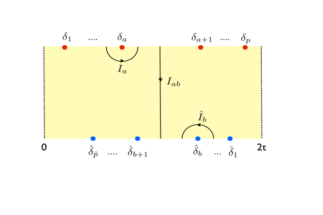
Figure III.4: The non-contractible 5-cycles in the circular-quiver geometries are fibrations of the two 2-spheres over the curves shown in this figure. $\Sigma$ is an annulus, so the dotted boundaries are identified.

In addition, as for the strip case, these geometries have a number of non-contractible five-cycles which can support D3-brane charge, that we expose in greater details here to be able to describe the subtelties of the charge conservation of the 5-form flux. These are fibrations of $S_{1}^{2}$ and $S_{2}^{2}$ over the three types of open curves $I_{a}$, $\hat{I}_{b}$ and $I_{ab}$ shown in figure III.4. Recalling that $S_{1}^{2}$ shrinks to a point in the lower boundary, and $S_{2}^{2}$ shrinks to a point in the upper boundary of the annulus, one deduces that the topology of these 5-cycles is as follows:

• ${\cal C}_{a}^{5}\equiv(S_{1}^{2}\times S_{1}^{2})\ltimes I_{a}$ and $\hat{\cal C}_{b}^{5}\equiv(S_{1}^{2}\times S_{1}^{2})\ltimes\hat{I}_{b}$ are topologically $S^{3}\times S^{2}$;

• ${\cal C}_{ab}^{5}\equiv(S_{1}^{2}\times S_{1}^{2})\ltimes I_{ab}$ are topologically $S^{5}$ .

Here $I_{ab}$ is a line segment which begins on the upper boundary of the annulus between the points $\delta_{a}$ and $\delta_{a+1}$ and ends on the lower boundary between the points $\hat{\delta}_{b}$ and $\hat{\delta}_{b+1}$. As shown in the figure, the orientation of the segments $I_{a},\hat{I}_{b}$ is chosen to be counter-clockwise, and for $I_{ab}$ from the upper annulus boundary to the lower boundary.

The D3-brane charges emanating from the five-brane singularities can be computed with the help of the general formulae of §III.2.2. Consider for example the $b$th NS5-brane stack which corresponds to the $z=\hat{\delta}_{b}$ singularity on the lower boundary of the annulus. Using $h_{1}^{D}={\cal A}_{1}+\bar{\cal A}_{1}$ and the expressions (III.2.23), (III.2.24) and (III.3.59) we find

$$\hat{N}^{(b)}_{3} =-\frac{2}{\pi\alpha^{\prime}}\hat{N}^{(b)}_{5}h_{1}^{D}|_{z={\hat{\delta}_{b}}}$$ (III.3.63)

$$=\hat{N}^{(b)}_{5}\,\sum_{a=1}^{p}N^{(a)}_{5}\,\left(\frac{i}{2\pi}\ln\bigg{[}\frac{\vartheta_{1}\left(\nu_{ab}|\tau\right)}{\vartheta_{1}\left(\bar{\nu}_{ab}|\tau\right)}\frac{\vartheta_{2}\left(\bar{\nu}_{ab}|\tau\right)}{\vartheta_{2}\left(\nu_{ab}|\tau\right)}\bigg{]}-\frac{4}{\pi\alpha^{\prime}}\varphi_{1}\right)\$$ (III.3.64)

where

$$i\nu_{ab}=\frac{\delta_{a}-\hat{\delta}_{b}}{2\pi}+\frac{i}{4}\ ,\qquad\tau=e^{-t}\ ,$$ (III.3.65)

and $\bar{\nu}$ is the complex conjugate of $\nu$. Likewise, one finds for the $a$th D5-brane:

$$N^{(a)}_{3} =\frac{2}{\pi\alpha^{\prime}}N^{(a)}_{5}h_{2}^{D}|_{z={\frac{i\pi}{2}+\delta_{a}}}$$ (III.3.66)

$$=N^{(a)}_{5}\,\sum_{b=1}^{\hat{p}}\hat{N}^{(b)}_{5}\,\left(-\frac{i}{2\pi}\ln\bigg{[}\frac{\vartheta_{1}\left(\nu_{ab}|\tau\right)}{\vartheta_{1}\left(\bar{\nu}_{ab}|\tau\right)}\frac{\vartheta_{2}\left(\bar{\nu}_{ab}|\tau\right)}{\vartheta_{2}\left(\nu_{ab}|\tau\right)}\bigg{]}-\frac{4}{\pi\alpha^{\prime}}\varphi_{2}\right)\ ,$$ (III.3.67)

where the arguments $\nu_{ab}$ are defined again by (III.3.65).

As has been discussed in the previous section, the D3-brane (Page) charge suffers from a gauge ambiguity which corresponds, in the above expressions, to the freedom in choosing the constants $\varphi_{1}$ and $\varphi_{2}$. In what follows, and until otherwise specified, we fix the gauge so that the potentials are continuous inside the fundamental domain $0\leq{\rm Re}z<2t$, and furthermore

$$C_{(2)} =0\qquad\rm{in}\ \ \,[0,\delta_{1}]\,\ \ \ \textrm{on the upper boundary},$$

$$B_{(2)} =0\qquad\rm{in}\,\ \ [\hat{\delta}_{1},2t]\,\ \ \ \textrm{on the lower boundary}.$$ (III.3.68)

The above choice can be motivated by considering the pinching limit $t\longrightarrow+\infty$ with $\delta_{a}$ and $\hat{\delta}_{b}$ kept fixed. In this limit the geometry degenerates to that of a linear quiver, and our gauge fixing agrees with the one adopted for linear quiver geometries.

Using the infinite-product expressions for the $\vartheta$-functions in (III.3.63) and (III.3.66), and fixing as just described $\varphi_{1}$ and $\varphi_{2}$, leads to the expressions

$${N^{(a)}_{3}}=N^{(a)}_{5}\sum_{b=1}^{\hat{p}}\hat{N}^{(b)}_{5}\Big{[}\sum_{n=0}^{+\infty}f(\hat{\delta}_{b}-\delta_{a}-2nt)-\sum_{n=1}^{+\infty}f(-\hat{\delta}_{b}+\delta_{a}-2nt)\Big{]}\ ,$$ (III.3.69)

and

$${\hat{N}^{(b)}_{3}}=\hat{N}^{(b)}_{5}\sum_{a=1}^{p}N^{(a)}_{5}\Big{[}\sum_{n=1}^{+\infty}f(-\hat{\delta}_{b}+\delta_{a}-2nt)-\sum_{n=0}^{+\infty}f(\hat{\delta}_{b}-\delta_{a}-2nt)\Big{]}\ ,$$ (III.3.70)

where ${N^{(a)}_{3}}$ is the D3-brane charge in the $a$th stack of D5-branes, ${\hat{N}^{(b)}_{3}}$ is the D3-brane charge in the $b$th stack of NS5-branes, and

$$f(x)=\frac{2}{\pi}\arctan(e^{x})\in[0,1]\ .$$ (III.3.71)

It can be easily verified that the above charges obey the sum rule

$$\sum_{a=1}^{p}N^{(a)}_{3}=-\sum_{b=1}^{\hat{p}}\hat{N}^{(b)}_{3}\ \equiv\ N\ .$$ (III.3.72)

In the pinching limit, where only the $n=0$ terms survive in the sums, all the $N^{(a)}_{3}$ are positive and all the $\hat{N}^{(b)}_{3}$ are negative numbers. For finite $t$, on the other hand, the numbers in each set can have either sign.

Next we consider the 5-cycles ${\cal C}_{ab}^{5}$. To associate to these 5-cycles a Page charge we must decide which (gauge-variant) 5-form to integrate. Take for instance the 5-form $\tilde{F}_{(5)}\equiv F_{(5)}+C_{(2)}\wedge H_{(3)}$, which obeys the non-anomalous Bianchi identity $d\tilde{F}_{(5)}=0$. This is globally defined only on the cycles ${\cal C}_{0b}^{5}$, since for all other choices of $a$, the gauge potential $C_{(2)}$ has a Dirac string singularity at the upper endpoint of $I_{ab}$. Put differently, $\int\tilde{F}_{(5)}$ would depend on the precise location of this upper endpoint unless $C_{(2)}=0$ in the corresponding boundary segment. By a similar reasoning one concludes that $\tilde{F}_{(5)}^{\prime}\equiv F_{(5)}-B_{(2)}\wedge F_{(3)}$ should be only integrated on the 5-cycles ${\cal C}_{a0}^{5}$. Both of these modified 5-forms can be integrated on the 5-cycle ${\cal C}_{00}^{5}$, which is picked out by our gauge fixing (III.3.2). Furthermore, the Page charge for this cycle does not depend on the choice of the modified 5-form since

$$\int_{{\cal C}_{00}^{5}}(\tilde{F}_{(5)}-\tilde{F}_{(5)}^{\prime})=\int_{{\cal C}_{00}^{5}}d\,(C_{(2)}\wedge B_{(2)})=0\ .$$ (III.3.73)

Let us denote the D3-brane charge for this special 5-cycle by $M$. If normalized appropriately, as in equation (III.2.23), $M$ must be an integer charge. We will now argue that this D3-brane charge is given by the following expression:

$$M=\sum_{a,b>0}N^{(a)}_{5}\hat{N}^{(b)}_{5}f(\hat{\delta}_{b}-\delta_{a})+\sum_{a,b\leq 0}N^{(a)}_{5}\hat{N}^{(b)}_{5}f(\delta_{a}-\hat{\delta}_{b})\ ,$$ (III.3.74)

where we here considered the universal cover of the annulus (i.e. the infinite strip), and extended the range of five-brane labels so that $-\infty<a<\infty$ is a label for the infinite array of D5-brane singularities from left to right, while $-\infty<b<\infty$ labels the corresponding array of NS5-brane singularities from right to left. Furthermore in this notation, $\delta_{a+np}\equiv\delta_{a}+2nt$ is the position of the $n$th image of the $a$th singularity on the upper strip boundary; likewise $\hat{\delta}_{b+m\hat{p}}\equiv\hat{\delta}_{b}-2mt$ corresponds to the $m$th image of the $b$th singularity on the lower strip boundary. The expression (III.3.74) can thus be written more explicitly as follows:

$$M =\sum_{a=1}^{p}\sum_{b=1}^{\hat{p}}N^{(a)}_{5}\hat{N}^{(b)}_{5}\Bigl{[}\sum_{m,n=0}^{\infty}f(\hat{\delta}_{b}-\delta_{a}-2nt-2mt)+\sum_{m,n=1}^{\infty}f(-\hat{\delta}_{b}+\delta_{a}-2nt-2mt)\Bigr{]}$$

$$=\sum_{a=1}^{p}\sum_{b=1}^{\hat{p}}N^{(a)}_{5}\hat{N}^{(b)}_{5}\sum_{s=1}^{\infty}s\Big{[}f(\hat{\delta}_{b}-\delta_{a}-2(s-1)t)+f(\delta_{a}-\hat{\delta}_{b}-2(s+1)t)\Big{]}\,.$$ (III.3.75)

A schematic explanation of the above expression is given in Figure III.5.

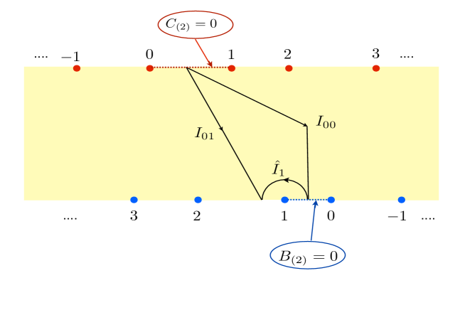
Figure III.5: The infinite array of 5-brane singularities on the universal cover of the annulus. The D5-branes on the upper boundary are labelled from left to right, and the NS5-branes on the lower boundary from right to left. The choice of gauge determines a fundamental domain, and a special 5-cycle ${\cal C}_{00}^{5}=I_{00}\times S_{1}^{2}\times S_{2}^{2}$. The D3-brane charge supported by this cycle is obtained by summing over all pairs of singularities with positive labels, and all pairs with non-positive labels, see equation (III.3.74).

To see that (III.3.74) is indeed right, let us consider a change of gauge which makes $B_{(2)}$ vanish on the boundary segment between the $b=1$ and the $b=2$ singularities. The privileged 5-cycle is now ${\cal C}_{01}^{5}$, and the corresponding D3-brane charge $M^{\prime}$ reads

$$M^{\prime}=\sum_{a>0,b>1}N^{(a)}_{5}\hat{N}^{(b)}_{5}f(\hat{\delta}_{b}-\delta_{a})+\sum_{a\leq 0,b\leq 1}N^{(a)}_{5}\hat{N}^{(b)}_{5}f(\delta_{a}-\hat{\delta}_{b})\ .$$ (III.3.76)

The difference $M^{\prime}-M$ is equal to $\hat{N}^{(3)}_{1}$, the number of D3-branes in the first NS5-brane stack, as one can check with the help of equation (III.3.70). This should be so since $I_{01}=I_{00}\oplus\hat{I}_{1}$, as illustrated in Figure III.5, and furthermore the corresponding Page charges, $M^{\prime}$ and $M+\hat{N}^{(3)}_{1}$, are given by integrals of the modified form $F_{(5)}+C_{(2)}\wedge H_{(3)}$ which does not depend on the choice of $B_{(2)}$ gauge.

This simple consistency check fixes almost uniquely the expression (III.3.74) for the charge $M$. To remove all doubts, we have also verified this formula numerically.

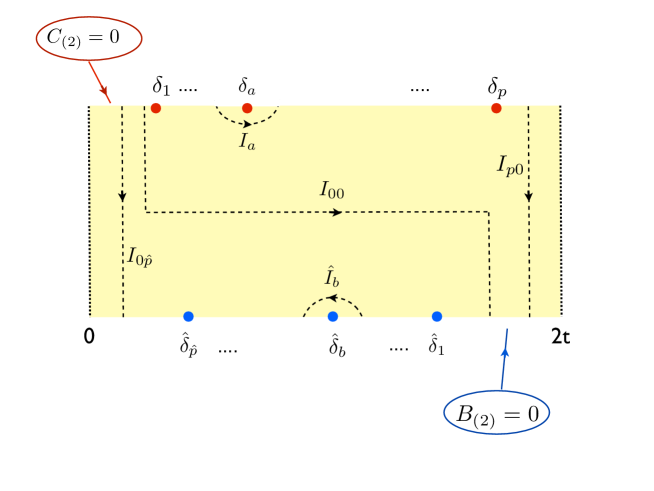
Figure III.6: A fundamental domain and the segments $I_{0\hat{p}}$ and $I_{p0}$ which correspond to the Page charge $L$. This is the number of winding D3-branes, which vanishes in the (pinching) limit of a linear quiver.

It will be convenient for our purposes here to trade $M$ for $L\equiv M-N$, where $N$ is the total charge carried by the D5-branes, see (III.3.72). The charge $L$ corresponds to the 5-form flux through the cycle ${\cal C}_{p0}^{5}$, or equivalently the cycle ${\cal C}_{0\hat{p}}^{5}$, depicted in Figure III.6. Simple manipulations give

$$L\ =\sum_{a=1}^{p}\sum_{b=1}^{\hat{p}}N^{(a)}_{5}\hat{N}^{(b)}_{5}\sum_{n=0}^{\infty}\sum_{m=1}^{\infty}\Bigl{[}f(\hat{\delta}_{b}-\delta_{a}-2nt-2mt)+f(-\hat{\delta}_{b}+\delta_{a}-2nt-2mt)\Bigr{]}$$

$$=\sum_{a=1}^{p}\sum_{b=1}^{\hat{p}}N^{(a)}_{5}\hat{N}^{(b)}_{5}\sum_{s=1}^{\infty}s\Big{[}f(\hat{\delta}_{b}-\delta_{a}-2st)+f(\delta_{a}-\hat{\delta}_{b}-2st)\Big{]}\,.$$ (III.3.77)

Below, we will identify $L$ with the number of winding D3-branes in a circular quiver. Consistently with this interpretation, $L$ can be seen to vanish in the pinching limit, $t\to\infty$ with $\delta_{a}-\hat{\delta}_{b}$, for all $a=1,\cdots p$ and $b=1,\cdots\hat{p}$, held finite and fixed.

To summarize the discussion, the 5-form flux as defined above on the various 5-cycles is conserved when deforming the segment of integration along the annulus. The segment $I_{00}$ plays a special role as one can trade the 5-form $F_{(5)}+C_{(2)}\wedge H_{(3)}$ for $F_{(5)}-B_{(2)}\wedge F_{(3)}$ or vice-versa, without changing the flux, to deform further the integration segment through the whole annulus. The 5-form fluxes or D3-charges defined this way are the $N^{(a)}_{3}$ and $\hat{N}^{(b)}_{3}$ charges for the D5 and NS5 singularities satisfying III.3.72(as in the case of the strip), plus a charge $L$ wrapping the annulus. These D3-charges, together with the D5-charges $N^{(a)}_{5}$ and NS5-charges $\hat{N}^{(b)}_{5}$, repackage all the $2(p+\hat{p})-1$ parameters of the supergravity solution III.3.52, as explained below.

III.3.3 Correspondence and 5-brane moves

In analogy with the linear quiver case, we define the linking numbers of the fivebranes as the Page charge per five-brane in each given stack:

$$l^{(a)}\equiv\frac{N^{(a)}_{3}}{N^{(a)}_{5}}\ ,\quad\hat{l}^{(b)}\equiv-\frac{\hat{N}^{(b)}_{3}}{\hat{N}^{(b)}_{5}}\ ,\qquad{\rm with}\ \ \ \sum_{a=1}^{p}N^{(a)}_{5}l^{(a)}=\sum_{b=1}^{\hat{p}}\hat{N}^{(b)}_{5}\hat{l}^{(b)}=N\ .$$ (III.3.78)

We here assume that these linking numbers are integer. Strictly-speaking, Dirac’s quantization condition only requires integrality of the total charge for each five-brane stack, so solutions with fractional linking numbers cannot be ruled out a priori as inconsistent. We will nevertheless discard this possibility, because we have no candidate SCFTs on the holographically dual side with fractional linking numbers. But the question deserves further scrutiny.

Next let us identify the above liking numbers with those in the brane construction of the circular quivers described in §II.3, by defining the following two partitions of $N$:

$$\rho =\Big{(}\overbrace{l^{(1)},l^{(1)},..,l^{(1)}}^{N_{5}^{(1)}},\overbrace{l^{(2)},l^{(2)},..,l^{(2)}}^{N_{5}^{(2)}},...,\overbrace{l^{(p)},l^{(p)},..,l^{(p)}}^{N_{5}^{(p)}}\Big{)}\ ,$$

$$\hat{\rho} =\Big{(}\overbrace{\hat{l}^{(1)},\hat{l}^{(1)},..,\hat{l}^{(1)}}^{\hat{N}_{5}^{(1)}},\overbrace{\hat{l}^{(2)},\hat{l}^{(2)},..,\hat{l}^{(2)}}^{\hat{N}_{5}^{(2)}},...,\overbrace{\hat{l}^{(\hat{p})},\hat{l}^{(\hat{p})},..,\hat{l}^{(\hat{p})}}^{\hat{N}_{5}^{(\hat{p})}}\Big{)}\ .$$ (III.3.79)

Together with the additional parameter $L$, we thus have the exact same data that was used to define the circular-quiver gauge theories $C_{\rho}^{\hat{\rho}}(SU(N),L)$ . Put differently, the supergravity parameters $\{\gamma_{a},\delta_{a}\}$ can be used to vary the charges $\{N_{5}^{(a)},N_{3}^{(a)}\}$, the parameters $\{\hat{\gamma}_{b},\hat{\delta}_{b}\}$ can be used to vary $\{\hat{N}_{5}^{(b)},\hat{N}_{3}^{(b)}\}$, and the annulus modulus $t$ controls the number $L$ of winding D3-branes. One of the charges is not independent because of the sum rule (III.3.78), but this agrees precisely with the fact that the supergravity solution is invariant under a common translation of all five-brane singularities on the boundary of the annulus.

The parameter counts on the supergravity and gauge-theory sides therefore match. The quiver data, on the other hand, had to obey a set of inequalities in order for the theory to flow to a non-trivial IR fixed point, see section II. We will show that the same inequalities are also obeyed on the supergravity side.

Note first that from the expressions (III.3.69) and (III.3.70), and the fact that $f(x)$ is a monotonic function, it follows that the linking numbers of the supergravity solutions are automatically arranged in decreasing order:

$$l^{(1)}>l^{(2)}>...>l^{(p)}\qquad{\rm and}\qquad\hat{l}^{(1)}>\hat{l}^{(2)}>...>\hat{l}^{(\hat{p})}\ .$$ (III.3.80)

From the brane-engineering point of view, it is possible to order the linking numbers by moving five-branes of the same type around each other in transverse space (this is obvious in the configuration of Figure II.4). We have argued in section §II that these moves do not change the infrared limit of the theory, up to decoupled free sectors. Such moves should thus be indistinguishable on the supergravity side.

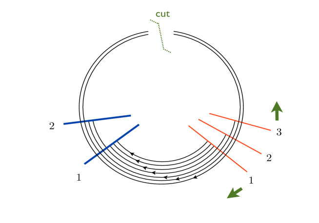
Figure III.7: Brane engineering of a circular quiver. Cutting open the circle on its high side leads to the linking-number assignements $\rho=(3,1,1)$ and $\hat{\rho}=(3,2)$ with $L=2$; the corresponding theory is $C_{\rho}^{\hat{\rho}}(SU(5),2)$. The green arrows indicate the elementary D5-brane moves described in the text. For instance, a rotation of the $3$rd D5-brane changes these assignments to $\rho^{\prime}=(3,3,1)$ and $\hat{\rho}^{\prime}=(4,3)$ with $L^{\prime}=3$.

Besides being arranged in decreasing order, the linking numbers of the field-theory side could be furthermore chosen to lie in the intervals $(0,\hat{k}]$ and $(0,k]$, with $k$ and $\hat{k}$ respectively the total numbers of D5-branes and NS5-branes, see (II.3.30) and (II.3.35). As was explained in §II.3, these inequalities were automatic if one chose to cut open the circular chain at a link of locally-minimal rank. We will now explain why the same argument goes through on the supergravity side.

To this end, consider the circular quiver of Figure III.7 defined by the triplet data $(\rho,\hat{\rho},L)$. Following the discussion in §II.3, to assign linking numbers to the five-branes we cut open the circular chain of D3-branes and then use the definitions (II.3.21). Clearly, the assignment is not unique since we are free to move one or several five-branes around the circle before cutting the chain. Let us focus, in particular, on the following two “elementary” moves:

• Move the (right-most) $k$th D5-brane anticlockwise, which produces the changes

  $$\Delta l_{k}=\hat{k}\ ,\ \ \Delta\hat{l}_{j}=1\ \ \ \forall\ j=1,\cdots\hat{k}\ ,\ \ \Delta L=l_{k}\ ;$$ (III.3.81)

• Move the (left-most) $1$rst D5-brane clockwise, which leads to the changes

  $$\Delta l_{1}=-\hat{k}\ ,\ \ \Delta\hat{l}_{j}=-1\ \ \ \forall\ j=1,\cdots\hat{k}\ ,\ \ \Delta L=\hat{k}-l_{1}\ .$$ (III.3.82)

These formulae translate the well-known fact that when a D5-brane crosses a NS5-brane it creates or destroys a D3-brane [12]. Similar formulae clearly hold for the mirror-symmetric moves of NS5-branes. The main point for us here is that the inequalities $l_{k}>0$ and $\hat{k}\geq l_{1}$ imply that $L$ is a “local” minimum with respect to elementary D5-brane moves. Likewise, $\hat{l}_{\hat{k}}>0$ and $k\geq\hat{l}_{1}$ imply that $L$ is a minimum with respect to elementary NS5-brane moves. One can thus impose the bounds (II.3.30) and (II.3.35) by choosing to cut the chain at a minimum of $L$.

This same line of argument applies to the supergravity side, where five-brane moves across the cut correspond to large gauge transformations. The elementary D5-brane moves are illustrated in Figure III.8. They correspond to shifting the boundary segment on which $C_{(2)}=0$ to a neighboring segment, on the right or left. Pushing for example this segment to the left leads to the following transformations of charges:

$$\Delta l^{(p)}=\hat{k}\ ,\ \ \Delta\hat{l}^{(b)}=N_{5}^{(p)}\ \ \ \forall\ b\ ,\ \ \Delta L=N_{5}^{(p)}l^{(p)}\ .$$ (III.3.83)

The last two equations follow from the expression for the linking numbers (see §III.2.2) and from the argument illustrated in Figure III.5. As for the first equation, it comes from the fact the $p$th D5-brane stack is replaced in the fundamental domain by the $0$th stack. On the universal cover of the annulus linking numbers (defined as the integrals over the 5-cycles ${\cal C}^{5}_{a}$ and $\hat{C}_{b}^{5}$) obey the periodicity conditions:

$$l_{a+np}=l_{a}-n\hat{k}\ ,\quad\hat{l}_{b+n\hat{p}}=\hat{l}_{b}-nk\ .$$ (III.3.84)

Thus replacing the $p$th stack by the $0$th stack changes the associated linking number by $\hat{k}$. Likewise, pushing the segment on which $C_{(2)}=0$ one step to the right leads to the following changes:

$$\Delta l^{(1)}=-\hat{k}\ ,\ \ \Delta\hat{l}^{(b)}=-N_{5}^{(1)}\ \ \ \forall\ b\ ,\ \ \Delta L=N_{5}^{(1)}(\hat{k}-l^{(1)})\ .$$ (III.3.85)

In this case the first D5-brane stack is replaced in the fundamental domain by the $(p+1)$th stack, as in Figure III.8.

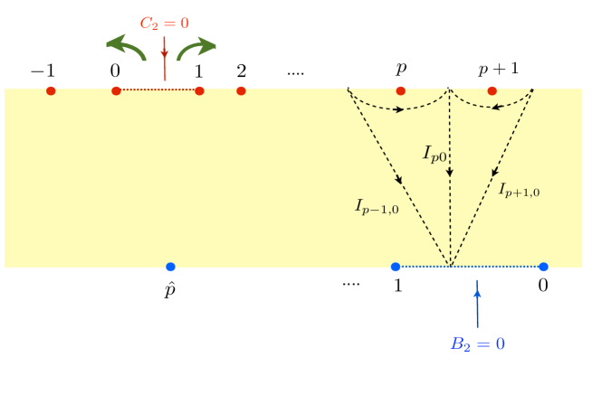
Figure III.8: Global gauge transformations corresponding to the elementary D5-brane moves described in the text. Pushing the boundary segment on which $C_{(2)}=0$ one step to the right corresponds to moving the first stack of D5-branes around the circular quiver clockwise once. Pushing this boundary segment to the left corresponds to moving the last D5-brane stack once in the anti-clockwise direction.

Equations (III.3.83) and (III.3.85) are the same as (III.3.81) and (III.3.82) when $N_{5}^{(p)}=N_{5}^{(1)}=1$. The large gauge transformations are in this case the counterpart of the elementary D5-brane moves. More generally, they describe the effect of moving the first and last stacks of D5-branes around the circular quiver. Requiring that $L$ be minimum under these moves implies that $\hat{k}-l^{(1)}\geq 0$ and $l^{(p)}>0$, as advertized. Likewise one shows that $k-\hat{l}^{(1)}\geq 0$ and $\hat{l}^{(p)}>0$, by requiring minimality under changes of the $B_{(2)}$ gauge. That such a minimum exists is guaranteed by the fact that $L$ is bounded below, and goes to infinity along with the separation $\delta_{1}-\hat{\delta}_{1}$. Note that in general there are several minima, so different triplets of data $(\rho,\hat{\rho},L)$ may correspond to one and the same supergravity solution, reflecting the redundancy we obtained in the circular quiver description when $L$ is only a local minimum (and not global).

Having established the inequalities (II.3.30) and (II.3.35), we now need to prove the inequalities (II.3.36) for the associated Young tableaux. In the brane constructions of §II.3 these inequalities guaranteed that all gauge groups have positive rank, i.e. that they are realized on D3-branes rather than anti-D3-branes. This is a condition for supersymmetry, so we expect it to be automatically satisfied on the supergravity side. The proof is straightforward but tedious, and we relegate it to appendix B.

III.4 Limiting geometries

In this section we discuss the solutions described above on the strip and the annulus, in regions of the parameters where the surface $\Sigma$ with the marked points on the boundary degenerates.
As a first case one may take the limit $(\delta_{a}-\delta_{a+1})\to 0$ with the other parameters held fixed. This simply merges the $a$th and $(a+1)$th stacks of D5-branes. Modulo the subtle issue of linking number quantization, this limit is thus rather dull. The more interesting limits are those of an infinite separation between stacks for the strip geometries and of an infinitely-thin ($t\to\infty$) or infinitely-fat annulus ($t\to 0$).

In the limit when the separation between 5-brane stacks is large, the size of the geometry in the ”deserted“ (or middle) region tends to zero and may be called a wormbrane geometry. The infinite separation corresponds to a ”pinching limit“ in which the wormbrane closes. In this case the strip solutions is split in two strip solutions, whereas the annulus degenerates to a strip ($t\to\infty$). We will show that these limits arise when one of the inequalities II.2.14, II.3.36 for the partitions $\rho,\hat{\rho}$ is saturated.

The other limit that we describe in the large $L$ limit ($t\to 0$) for the annulus solutions which corresponds to a large number of D3-branes wrapping the circle in the brane picture. We call it the fat annulus because the volume of the annulus diverges in this limit. As we will see, this limit operates the smearing of the 5-branes.

After discussing these limits we analyse the regime of parameters in which the supergravity description can be used.

III.4.1 Wormbrane limits

The splitting strip :

The limits for the linear quiver geometries in which one or more of the inequalities contained in the statement $\rho^{T}>\hat{\rho}$ become equalities, are of special significance.

As explained at the end of appendix B one inequality can be saturated in two different limits:
(i) when $\delta_{a}\rightarrow+\infty$ for $a=I+1,I+2,...,p$ and $\hat{\delta}_{b}\rightarrow+\infty$ for $b=1,2,...,J$, or
(ii) when $\delta_{a}\rightarrow-\infty$ for $a=1,2,...,I$ and $\hat{\delta}_{b}\rightarrow-\infty$ for $j=J+1,J+2,...,\hat{p}$.
In the supergravity solution, these two limits are related by a singular coordinate transformation corresponding to a large (infinite) translation of the strip.

This limit corresponds to detaching a subset of fivebrane singularities and moving them off to infinity on the strip. On the field theory side, on the other hand, the quiver gauge theory breaks up into two (or more) pieces, which are connected by a “weak node”, i.e. a node of the quiver diagram for which the gauge group has rank much smaller than the ranks of all other gauge groups. We will now make this statement more explicit.

Consider the limit (i) in which $\delta_{a}\rightarrow+\infty$ for $a=I+1,I+2,...,p$ and $\hat{\delta}_{b}\rightarrow+\infty$ for $b=1,2,...,J$ (the limit (ii) is as we have just argued equivalent). In this limit the charges (III.2.36) for the fivebrane stacks at finite $z$ reduce to:

$$N^{(a)}_{D3} =k^{(a)}\sum_{b=J+1}^{\hat{p}}\hat{N}^{(b)}_{NS5}+N^{(a)}_{D5}\sum_{b=1}^{J}\hat{N}^{(b)}_{NS5}\frac{2}{\pi}\arctan(e^{\hat{\delta}_{b}-\delta_{a}})\ ,\qquad a=I+1,...,p$$

$$\hat{N}^{(b)}_{D3} =\hat{\hat{k}}^{(b)}\sum_{a=1}^{I}N^{(a)}_{D5}\frac{2}{\pi}\arctan(e^{\hat{\delta}_{b}-\delta_{a}})\ ,\qquad\qquad\qquad b=1,...,J\ .$$ (III.4.86)

The extra contribution in $N^{(a)}_{D3}$ coming from the branes located at $\infty$ is actually irrelevant, as it can be removed by an appropriate gauge transformation of $B_{2}$. This corresponds to choosing the gauge so that $B_{2}=0$ on the segment $(\hat{\delta}_{J+1},\hat{\delta}_{J})$. In this way, a solution with $I$ D5-branes stacks and $(\hat{p}-J)$ NS5-brane stacks is detached from the rest of the geometry.

More generally, if we keep also track of the fivebranes moving off to infinity, we find a supergravity solution which consists of two geometries of type $AdS_{4}\ltimes K$ and $AdS_{4}\ltimes K^{\prime}$, connected by a narrow bridge, as illustrated in figure III.9. The space $AdS_{4}\ltimes K$ corresponds to keeping only the stacks $a=1,2,...,I$ , $b=J+1,J+2,...,\hat{p}$, while the space $AdS_{4}\ltimes K^{\prime}$ is the solution obtained if we only keep the fivebrane stacks $a=I+1,I+2,...,p$ , and $b=1,2,...,J$. Saturating the relation $\rho^{T}\geq\hat{\rho}$ corresponds to eliminating all D3-branes in the intermediate region. It can be checked indeed that, in the limit, the D3-brane charge is separately conserved in the two regions.

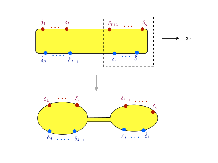
Figure III.9: Schematic drawing of the factorization limit of fivebrane singularities discussed in the text. The lower picture is meant to show the actual size of the strip geometry. The background consists of two, $AdS_{4}\ltimes K$ and $AdS_{4}\ltimes K^{\prime}$, solutions coupled through a narrow $AdS_{5}\times S^{5}$ bridge. The curvature of the narrow bridge is larger than the curvature in the rest of the geometry, but can be small enough so as to ignore quantum gravity corrections. The configuration resembles therefore a wormhole (or worm-brane).

We can check that the partitions corresponding to these two solutions are exactly the ones obtained by the splitting of ($\rho$ , $\hat{\rho}$) into two subpartitions by the saturation of the condition (B.13). These partitions are explicitly :

$$\rho_{L} = \Big{(}\underbrace{l_{1}-\sum_{b=1}^{J}\hat{N}_{b},...,l_{1}-\sum_{b=1}^{J}\hat{N}_{b}}_{N_{1}},...,\underbrace{l_{I}-\sum_{b=1}^{J}\hat{N}_{b},...,l_{I}-\sum_{b=1}^{J}\hat{N}_{b}}_{N_{I}}\Big{)}$$

$$\hat{\rho}_{L} = \Big{(}\underbrace{\hat{l}_{J+1},...,\hat{l}_{J+1}}_{\hat{N}_{J+1}},...,\underbrace{\hat{l}_{\hat{p}},...,\hat{l}_{\hat{p}}}_{\hat{N}_{\hat{p}}}\Big{)}$$ (III.4.87)

and

$$\rho_{R} = \Big{(}\underbrace{l_{I+1},...,l_{I+1}}_{N_{I+1}},...,\underbrace{l_{p},...,l_{p}}_{N_{p}}\Big{)}$$

$$\hat{\rho}_{R} = \Big{(}\underbrace{\hat{l}_{1}-\sum_{a=1}^{I}N_{a},...,\hat{l}_{1}-\sum_{a=1}^{I}N_{a}}_{\hat{N}_{1}},...,\underbrace{\hat{l}_{J}-\sum_{a=1}^{I}N_{a},...,\hat{l}_{J}-\sum_{a=1}^{I}N_{a}}_{\hat{N}_{J}}\Big{)}$$ (III.4.88)

where the indices L, R refer to the left and right parts of the split quiver. The linking numbers have been here gauge transformed so as to make them agree, for each sub-quiver separately, with our earlier conventions. So the splitting of the quiver corresponds precisely to the factorization of the bulk geometry, confirming once again the holographic duality map.

The pinched annulus :

In the case of the annulus we study the limit of infinite length $t\to\infty$.
When taking the limit $t\to\infty$ one must decide what to do with the positions, $\{\delta_{a}\}$ and $\{\hat{\delta}_{b}\}$, of the five-brane singularities. If the number of singularities is kept fixed then, since $\delta_{a}-\delta_{a+p}=\hat{\delta}_{b}-\hat{\delta}_{b+\hat{p}}=2t$, at least one of the intervals $\delta_{a}-\delta_{a+1}$ with $a\in[1,p]$, and at least one interval $\hat{\delta}_{b}-\hat{\delta}_{b+1}$ for some $b\in[0,\hat{p}-1]$ should become infinite in the limit. Without loss of generality, we take these divergent separations to correspond to $a=p$ and $b=0$. From the expression (III.3.2) we conclude that $L\to 0$ in this limit, so that the circular quiver degenerates to a linear quiver. If more than one interval diverges, the linear quiver breaks up further into disjoint linear quivers as just described.

In the two limits we have described, the geometry describes what one may call a “worm-brane”. A schematic representation of this space-time is given in Figure III.10 for the for the $L\rightarrow 0$ case. A highly-curved $AdS_{5}\times S_{5}$ throat from a bridge between either two compact spaces $K_{6},K^{\prime}_{6}$ (strip), or between two distinct points of the same compact space $K_{6}$(annulus), forming a handle. The wormhole entrances are three-dimensional extended objects, whence the name “worm-brane”.

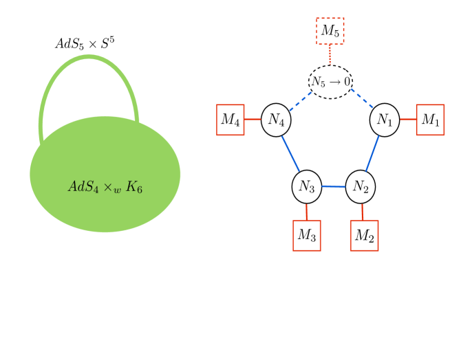
Figure III.10: Breaking up of a circular quiver as described in the text. On the left, the ten-dimensional geometry describes a wormhole whose entrances are extremal D3-branes. An example of a dual gauge theory is illustrated on the right: a gauge-group factor with vanishing rank opens up the chain into a linear quiver.

From the perspective of the gauge theory, the pinching-limit geometries describe quivers with a gauge-group factor whose rank is much smaller than all other ranks. Taking this rank formally to zero opens up the circular chain or cut the linear chain in two pieces, and decouples the corresponding fundamental hypermultiplets, see Figure III.10. In general, the limiting geometries are smooth except when one sends a set of stacks of the same type infinitely far from all other stacks. This corresponds in gauge theory to the decoupling of free hypermultiplets from the end-points of a linear quiver. The geometry with five-branes of only one type is singular (it corresponds to having either $h_{1}=0$ or $h_{2}=0$), consistently with the fact that free hypermultiplets should have no smooth supergravity dual.

We have not discussed the case of domain wall solutions corresponding to defect SCFT. The case is identical to the linear quiver geometries. The same wormbrane limit is possible, corresponding to having a weak node. The two separated solutions obtained in this limit have only one $AdS_{5}\times S^{5}$ asymptotic region (the other is capped off) and corresponds to solutions described in [83], with the gauge theory duals being SYM on a half-space with a 3d boundary SCFT.

Let’s just mention that the intuition that one could obtain two separated defect SCFT in a wormbrane limit is wrong. The wormbrane limit corresponds to a weak node in the quiver, not to a separation in the direction transverse to the defect. The separation between ”different“ 3d defects in SYM is actually irrelevant as we consider only the infrared limit of such theories.

III.4.2 Large-$L$ limit and M2 branes

The second interesting limit of the circular-quiver solutions of section §III.3 is the limit $t\to 0$, $\delta_{a},\hat{\delta}_{b}\to 0$ with $\delta_{a}/t,\hat{\delta}_{b}/t$ held fixed. As we will see, this is the limit of a very large number, $L$, of winding D3-branes, in which the five-branes are effectively smeared, and the solution reduces to the near-horizon geometry of M2-branes at a $Z_{k}\times Z_{\hat{k}}$ orbifold singularity.

To compute the geometry in this limit we use the asymptotic behavior of the theta functions when $e^{i\pi\tau}=e^{-t}\to 1$, or equivalently $e^{i\pi\tilde{\tau}}=e^{-i\pi/\tau}=e^{-\pi^{2}/t}\to 0$. One finds in this limit

$${\vartheta_{1}(\nu|\tau)\over\vartheta_{2}(\nu|\tau)}=-i{\vartheta_{1}(\nu\tilde{\tau}|\tilde{\tau})\over\vartheta_{4}(\nu\tilde{\tau}|\tilde{\tau})}\,=\ -2\,e^{-\pi^{2}/4t}\,{\rm sinh}({\pi^{2}\nu/t})+{\cal O}(e^{-9\pi^{2}/4t})\ ,$$ (III.4.89)

where the second equality follows from the expressions of the theta functions as infinite sums. The formula simplifies further if ${\rm Re}(\nu)\not=0$, in which case the hyperbolic sine can be replaced by an exponential. Inserting (III.4.89) in (III.3.59), and recalling that $2\pi{\rm Re}(\nu_{a})=\pi/2-{\rm Im}(z)$ and $2\pi{\rm Re}(\hat{\nu}_{b})={\rm Im}(z)$, finally gives

$${\cal A}_{1}=\sum_{a=1}^{p}\gamma_{a}\,{\pi\over 2t}z+\varphi_{1}\ ,\ \quad{\cal A}_{2}=i\sum_{b=1}^{\hat{p}}\hat{\gamma}_{b}\,{\pi\over 2t}(z-{i\pi\over 2})+i\varphi_{2}\ ,$$ (III.4.90)

where we have absorbed some irrelevant constants in the arbitrary phases $\varphi_{1}$ and $\varphi_{2}$. This approximation breaks down at a distance $\sim t$ from the annulus boundaries, where the linear dependence is replaced by the rapidly-oscillating $\log\,{\rm sinh}$ function.

The first thing to note is that, away from the boundaries, the harmonic functions depend only on three parameters: $t$ and the total numbers of five-branes, $k=\sum\gamma_{a}$ and $\hat{k}=\sum\hat{\gamma}_{b}$. The precise locations of the five-brane singularities do not matter, as if these were smeared. It is convenient to scale out the $t$-dependence by redefining the annulus coordinate as follows: $2\pi z=2tx+i\pi^{2}y$, so that $x\in[0,2\pi)$ and $y\in[0,1]$. In terms of these coordinates, the holomorphic functions read

$${\cal A}_{1}=k\,({x\over 2}+i{\pi^{2}y\over 4t})\ ,\ \quad{\cal A}_{2}=i\hat{k}\,\left({x\over 2}-\pi+i{\pi^{2}(y-1)\over 4t}\right)\ ,$$ (III.4.91)

where we have here chosen $\varphi_{1}$ and $\varphi_{2}$ so as to impose the canonical gauge condition (III.3.2), which is really $C_{2}|_{(x,y)=(0,1)}=0$ and $B_{2}|_{(x,y)=(2\pi,0)}=0$ in this smearing limit. Inserting these functions in the general form of the solution, see §III.2.1, gives the Einstein-frame metric (we recall that $\alpha^{\prime}=4$):

$$ds^{2}=R^{2}g(y)^{1\over 4}\left[ds^{2}_{AdS_{4}}+y\,ds^{2}_{S^{2}_{1}}+(1-y)ds^{2}_{S^{2}_{2}}\right]+R^{2}g(y)^{-{3\over 4}}\left[{4t^{2}\over\pi^{4}}dx^{2}+dy^{2}\right]\ ,$$

$${\rm with}\quad R^{4}=\pi^{4}\,{{k\hat{k}}\over t^{2}}\ ,\qquad{\rm and}\quad g(y)=y(1-y)\ .$$ (III.4.92)

Furthermore, the dilaton and the non-vanishing gauge fields read:

$$e^{2\phi}=\frac{\hat{k}}{k}\sqrt{\frac{1-y}{y}}\ ,\qquad C_{(4)}=R^{4}\left({6tx\over\pi^{2}}\,\omega^{0123}+y^{2}(y-{3\over 2})\,\omega^{4567}\right)\ ,$$

$$B_{(2)}=2\hat{k}(2\pi-x)\,\omega^{45}\ ,\qquad C_{(2)}=-2kx\,\omega^{67}\ .$$ (III.4.93)

As already noted, this solution only depends on three integer parameters: the numbers $k$ and $\hat{k}$ of five-branes, and the modulus $t$ of the annulus which can be traded for the number of winding D3-branes via the formula (III.3.2),

$$L\,=\,\frac{k\hat{k}}{2t^{2}}\,\int_{0}^{+\infty}du\,u\,\frac{2}{\pi}\arctan(e^{-u})\,=\,\frac{\pi^{2}}{32}\,\frac{k\hat{k}}{t^{2}}\ .$$ (III.4.94)

One may also compare (III.3.2) to the formula (III.3.2) for the charge $M=L+N$, where $N$ gives the number of D3-branes emanating from five-branes. Since the summands in these two expressions differ by terms of order $t^{2}$, we conclude that $N\sim k\hat{k}$ as $t\to 0$. Thus the number of winding D3-branes far exceeds, in this limit, the number of D3-branes that end on the five-branes.

Not surprisingly, after having effectively smeared the five-branes, the solution has a Killing isometry under translations of the coordinate $x$. To be sure, $x$ enters in the expressions for $B_{(2)}$ and $C_{(2)}$ but this is a gauge artifact since the 3-form field strengths are $x$-independent. One may thus T-dualize the circle parametrized by $x$, using Buscher’s rules [91], to find a solution of type-IIA supergravity. This can be then lifted to eleven dimensions – the details of these calculations are given in appendix C. The final result for the eleven-dimensional metric is

$$ds_{{\rm M-theory}}^{2} ={\bar{R}^{2}}ds^{2}_{AdS_{4}}+\bar{R}^{2}\Big{[}4d\alpha^{2}+\sin^{2}\alpha\,ds^{2}_{S^{3}/\mathbb{Z}_{\hat{k}}}+\cos^{2}\alpha\,ds^{2}_{S^{3}/\mathbb{Z}_{k}}\Big{]}\ ,$$

$$ds^{2}_{S^{3}/\mathbb{Z}_{\hat{k}}} =d\theta_{1}^{2}+d\phi_{1}^{2}+4dx^{2}-4\cos\theta_{1}dxd\phi_{1}\ ,$$

$$ds^{2}_{S^{3}/\mathbb{Z}_{k}} =d\theta_{2}^{2}+d\phi_{2}^{2}+4dv^{2}-4\cos\theta_{2}dvd\phi_{2}\ ,$$ (III.4.95)

where $x$ and $v$ are angle coordinates with periodicities $x=x+2\pi/\hat{k}$ and $v=v+2\pi/k$, while the radius of $AdS_{4}$ is $\bar{R}^{2}=(2^{5}\pi^{2}k\hat{k}L)^{1/3}$.

This is the metric of $AdS^{4}\times S^{7}/(\mathbb{Z}_{k}\times\mathbb{Z}_{\hat{k}})$ with the two orbifolds acting on the two 3-spheres in $S^{7}$. The solution furthermore carries $L$ units of four-form flux. It can be recognized as the near-horizon geometry of $L$ M2-branes sitting at the fixed point of the orbifold $(\mathbb{C}^{2}/\mathbb{Z}_{\hat{k}})\times(\mathbb{C}^{2}/\mathbb{Z}_{k})$, where the orbifold identifications are

$$(z_{1},\bar{z}_{2})=e^{2i\pi/\hat{k}}(z_{1},\bar{z}_{2})\quad{\rm and}\quad(z_{3},\bar{z}_{4})=e^{2i\pi/k}(z_{3},\bar{z}_{4})\ .$$

Note that the two-forms $B_{(2)}$ and $C_{(2)}$ become, after the T-duality and the lift, part of the metric. This is in line with the fact that D5-branes transform (to D6-branes and then) to Kaluza-Klein monopoles, while T-duality in a transverse dimension maps the NS5-branes to ALE spaces with singularities of $A_{n}$ type [92, 31].

The superconformal field theories that are dual to M theory on $AdS^{4}\times S^{7}/(\mathbb{Z}_{k}\times\mathbb{Z}_{\hat{k}})$ are close relatives of the ABJM theory [1, 49] that have been analyzed by many authors, see for example [86, 87, 5, 30, 35, 90]. We will discuss them in more detail in the following section. Let us here only quote their free energy $F=-\log|Z|$ on the 3-sphere. Using the general formula of [35] one finds

$$F\,=\,L^{3/2}\sqrt{\frac{2\pi^{6}}{27\,{\rm Vol}_{7}}}\,=\,\frac{\pi}{3}\sqrt{2k\hat{k}}\,L^{3/2}\ ,$$ (III.4.96)

where ${\rm Vol}_{7}$ is the volume of the compact (Sasaki-Einstein) manifold whose metric is normalized so that $R_{ij}=6g_{ij}$. In the case at hand, this is the unit-radius seven sphere with orbifold identifications, so that ${\rm Vol}_{7}={\pi^{4}}/{3k\hat{k}}$.

As a check of our formulae, we may compute this free energy on the type-IIB side.

The on-shell IIB action can be computed via a consistent truncation to pure four-dimensional gravity with unit $AdS_{4}$ metric multiplied by a 6d volume factor. We defer the explicit computation of the regularized action to the next chapter, where it plays a central role, and just quote the explicit formula

$$S_{\rm IIB}=-\frac{1}{(2\pi)^{7}(\alpha^{\prime})^{4}}\left(\frac{4}{3}\pi^{2}\right)(-6){\rm vol}_{6}\ ,$$ (III.4.97)

where for the solutions of interest

$${\rm vol}_{6}=-16(4\pi)^{2}t\int_{0}^{2\pi}\hskip-2.84526ptdx\int_{0}^{1}\hskip-2.84526ptdy\,h_{1}h_{2}\,\partial_{z}\partial_{\bar{z}}(h_{1}h_{2})\ .$$ (III.4.98)

Plugging in the harmonic functions $h_{1}=-i({\cal A}_{1}-\bar{\cal A}_{1})$ and $h_{2}={\cal A}_{2}+\bar{\cal A}_{2}$, and performing the integrals gives

$$S_{\rm IIB}=\frac{\pi^{4}}{48}\frac{k^{2}\hat{k}^{2}}{(2t)^{3}}=\frac{\pi}{3}\sqrt{2k\hat{k}}\,L^{3/2}$$ (III.4.99)

in perfect agreement with the result of M theory.

To summarize, we have shown here that when $L$ is large our solutions approach smeared backgrounds dual to M theory on $AdS^{4}\times S^{7}/(\mathbb{Z}_{k}\times\mathbb{Z}_{\hat{k}})$. In this limit the information about the positions of the five-branes is lost, and following [93, 94] its reinstatement would require non-trivial backgrounds for the wrapped-membrane field. The essential topological features of the background can be, however, in principle encoded more simply, as 3-form torsion of the M-theory orbifold [30, 88, 89, 90]. Note that, contrary to the $\mathcal{N}\geq 6$ ABJ(M) cases studied in [1, 49], the orbifolds considered here are not freely-acting on S$\hskip-1.42262pt\,{}^{7}$, and one would need to resolve their singularities. It would be interesting to work out the precise match of the torsion with the quiver data, and see how the constraints on the triplet $(\rho,\hat{\rho},L)$ arise from the M-theory side.

III.4.3 Supergravity regimes of parameters

A interesting question to ask is : In which regime of parameters can we trust the supergravity solutions described in this chapter ? The answer should naïvely be that the supergravity description always breaks down, due to the presence of D5-brane singularities where the curvature diverges and NS5-brane singularities where the dilaton diverges (to $+\infty$). However we know that these singularities must be cured by string corrections. It is sensible to assume that as long as the regions of large curvature or large dilaton are confined to the close vicinity of the 5-branes in $\Sigma$ the supergravity description can be used to answer some questions and do computations in which the 5-branes contribution is subdominant.

Having evacuated the question of the 5-branes we want to find the regime of parameters where the radius of curvature is large compared to the Planck length (and string length) and the dilaton diverges to $-\infty$ (small string coupling). These are the conditions for the quantum loop corrections and string corrections to be supressed. This goes down to demanding

$$R_{r.c.}>>1\quad,\quad e^{2\phi}<<1\quad,$$ (III.4.100)

where $R_{r.c.}$ is the radius of curvature in string units (and $\phi$ is the dilaton).

Verifying these conditions is not straightforward, because of the complexity of the parameter dependence of the supergravity solutions. By analogy with the Maldacena setup (see §I.2) we may demand a large 5-form flux or large number of D3-branes in the geometry. Fo the linear quivers $T^{\rho}_{\hat{\rho}}(SU(N))$ it corresponds to the large $N$ limit. For circular quivers $C_{\hat{\rho}}^{\rho}(SU(N),L)$ it can also be the large $N$ limit, however in this limit the circular quiver geometry degenerates into a linear quiver geometry (when $N>>L$ the node of the quiver with rank $L$ is a weak node and the circular quiver breaks into a linear one, as discussed above). The interesting limit of large D3-brane flux for circular quivers is then the large $L$ limit studied in the last subsection.

Taking the large $N$ limit for linear quiver geometries, the formulas III.2.39III.2.36 implies that there is a couple $(a,b)$ with $N_{5}^{a}\sim N^{\alpha}$, $\hat{N}_{5}^{b}\sim N^{\beta}$ and $e^{\hat{\delta}_{b}-\delta_{a}}\sim N^{1-\alpha-\beta}$ with $0\leq\alpha,\beta\leq 1\leq\alpha+\beta$. This in turn implies that in the region between the two 5-brane stacks $a$ and $b$ the harmonic functions scale like

$$h_{1}\sim N^{\frac{1+\alpha-\beta}{2}}\quad,\quad h_{2}\sim N^{\frac{1+\beta-\alpha}{2}}\ .$$ (III.4.101)

Then using the formulas of §III.2.1 describing the solutions, we obtain that the Einstein metric scales like $g_{\mu\nu}\sim N^{1/2}$ independently of $\alpha,\beta$ and the dilaton scales $e^{2\phi}\sim N^{\beta-\alpha}$. The string frame metric $g_{\mu\nu}^{(srt)}=e^{\phi}g_{\mu\nu}$ scales $g_{\mu\nu}^{(srt)}\sim N^{\frac{1+\beta-\alpha}{2}}$. We obtain

$$R_{r.c.}^{2}\sim N^{\frac{1+\beta-\alpha}{2}}\quad,\quad e^{2\phi}\sim N^{\beta-\alpha}\ .$$

The condition $R_{r.c.}>>1$ is always satisfied, except in the special case $(\alpha,\beta)=(1,0)$, whereas the condition $e^{2\phi}<<1$ needs $\alpha>\beta$, which can be traced back to the condition that the number of D5-branes in the stack $a$ has to be (hierarchicaly) larger than the number of NS5-branes in the stack $b$.
This is not surprizing : the large $N$ conditions ensures that the radius of curvature is large, as in the Maldacena setup, and the larger number of D5-branes ensures that the string coupling is small in the geometry (remember that the dilaton goes to $+\infty$ near the NS5-branes and to $-\infty$ near the D5-branes).

Using S-duality one obtains a dual supergravity solution with NS5-brane and D5-brane stacks exchanged. The parameters $\alpha$ and $\beta$ are exchanged in the process. This means that if $\alpha<\beta$, we can use the S-dual solution where the conditions for the supergravity regime are verified. This leaves us with only two problematic regimes : $(\alpha,\beta)=(1,0)$ and $\alpha=\beta$. As we will see in chapter IV, in the latter ”bad“ regime one may use the supergravity solutions and obtain some correct computations.

We conclude that the supergravity regime for linear quiver theories is generically the large $N$ limit and small ratio $\frac{\hat{k}}{k}$ of the total number of NS5-branes $\hat{k}$ over the total number of D5-branes $k$.

$$N>>1\quad,\quad\frac{\hat{k}}{k}<<1\ ,$$ (III.4.102)

with the possibility to use S-dual solutions if $\frac{\hat{k}}{k}>>1$.
Note that the parameters $k,\hat{k}$ and $N$ are not really independent. They obey for instance $k,\hat{k}\leq N\leq k\hat{k}$, as can be seen from the explicit expressions III.2.36 III.2.39. This shows that the condition $\frac{\hat{k}}{k}<<1$ is actually enough because it implies $N>>1$.

The existence of a regime in which the supergravity calculations can be trusted (when the 5-brane contributions can be ignored) is to be contrasted with the situation on the gauge theory side where there is a priori no accessible regime (infinitely strongly coupled gauge theories).

The situation for the $C_{\hat{\rho}}^{\rho}(SU(N),L)$ circular quiver solutions in the large $L$ limit (with $N<<L$) is different. The number $L$ of D3-branes wraping the annulus is independent from the numbers of 5-branes. From the analysis of the last subsection §III.4.2, we see that the radius of curvature (in string frame) is given by $R_{r.c.}^{4}\sim L\hat{k}/k$ in all directions, except in the $x$ direction wrapping the annulus (and on a small vicinity of the upper boundary where the smeared D5-branes sit) with $R_{r.c.}^{4}\sim L\hat{k}/k$, $R_{r.c.}^{x\ 4}\sim\hat{k}^{4}/L$. The dilaton goes like $e^{2\phi}\sim\hat{k}/k$ everywhere. This implies that the regime of parameters when supergravity can be used is

$$\frac{\hat{k}}{k}<<1\quad,\quad 1<<\frac{L\hat{k}}{k}<<\frac{\hat{k}^{5}}{k}\ .$$ (III.4.103)

Because of S-duality one can also use the supergravity solution in the regime III.4.103 with $k\leftrightarrow\hat{k}$. Again there is a priori no weak-coupling regime on the gauge theory side.

The experience of the AdS/CFT correspondence lets us think that the presence of supergravity regimes for the solutions dual to the linear and circular quivers may be an indication that there is a corresponding weak-coupling regime on the gauge theory side, for dual SCFTs that remains to find. The orbifold duality between Yang-Mills theories and Chern-Simons-Matter theories that we present in chapter V may be the answer to this question, however the situation is not really clear as the orbifold duality is not a duality at the quantum level.

Chapter IV Testing the correspondence : free energy calculations

In this chapter we provide further quantitative consistency checks of this $AdS_{4}/CFT_{3}$ correspondence by verifying the GKPW relation I.2.13 (reviewed in section I.2) for the partition function [25, 28] in the leading large $N$ limit :

$$\left|Z_{\rm CFT}\right| =e^{-S_{\rm gravity}}\ ,\quad\textrm{i.e.}\quad F_{\rm CFT}=S_{\rm gravity}\ ,$$ (IV.0.1)

where $Z_{\rm CFT}$ is a CFT partition function on $S^{3}$, $F_{\rm CFT}:=-\ln|Z_{\rm CFT}|$ is the free energy, and $S_{\rm gravity}$ is the action for the type IIB supergravity holographic dual to the CFT.

We concentrate on a class of 3d $\mathcal{N}=4$ linear quiver SCFTs $T^{\rho}_{\hat{\rho}}[SU(N)]$ in which the numbers of 5-branes grow as fractional powers of $N$ (see below).

On the CFT side, we take the large $N$ limit of the $S^{3}$ partition functions of [32, 23], evaluated at the conformal point. On the gravity side, we evaluate the gravity action on the linear quiver solutions presented in section III.2. The action is evaluated on the (regularized) euclidean $AdS_{4}$ spacetimes, whose conformal boundary is $S^{3}$. The radius $r$ of $S^{3}$ provides a (IR) cutoff and makes it possible to compute the partition function using the localization techniques ([15]), however the $r$ dependence disappears from the final result. We find that in both cases the leading contribution of the free energy in the large $N$ limit scales as

$$F\sim N^{2}\ln N+{\cal O}(N^{2})\ .$$

As we will see, on the CFT side $N^{2}\ln N$ comes from the asymptotic behavior of the Barnes $G$-function. On the gravity side, a factor of $N^{2}$ comes from the local scaling of the supergravity Lagrangian, and an extra $\ln N$ comes from the size of the geometry.

Summary of results :

Our findings are summarized as follows.

• The simplest prototypical example is the $T[SU(N)]$ theory, which is a $T^{\rho}_{\hat{\rho}}[SU(N))]$ theory with

  $$\rho=\hat{\rho}=\big{[}\overbrace{1,1,...,1}^{N}\big{]}\ .$$ (IV.0.2)

  In this case we find

  $$F_{\rm CFT}=S_{\rm gravity}=\frac{1}{2}N^{2}\ln N+\mathcal{O}(N^{2})\ .$$ (IV.0.3)

• More generally we consider the case $\hat{p}=1$, i.e.,

  $$\begin{split}\rho&=\Big{[}\overbrace{l^{(1)},l^{(1)},..,l^{(1)}}^{N_{5}^{(1)}},\ \overbrace{l^{(2)},l^{(2)},..,l^{(2)}}^{N_{5}^{(2)}},\ ...\ ,\ \overbrace{l^{(p)},l^{(p)},..,l^{(p)}}^{N_{5}^{(p)}}\Big{]}\ ,\\ \hat{\rho}&=\Big{[}\overbrace{\hat{l},\hat{l},..,\hat{l}}^{\hat{N}_{5}}\Big{]}\ .\end{split}$$ (IV.0.4)

  We take the scaling limit

  $$N_{5}^{(a)}=N^{1-\kappa_{a}}\gamma_{a},\quad l^{(a)}=N^{\kappa_{a}}\lambda^{(a)},\quad\hat{N}_{5}=N\hat{\gamma}\ ,$$ (IV.0.5)

  where we take $N$ large, while keeping $\kappa_{a},\lambda^{(a)},\gamma_{a},\hat{\gamma}$ finite.

  We require

  $$\kappa_{a-1}\geq\kappa_{a},\quad 0\leq\kappa_{a}<1,\quad\textrm{for all }a\ .$$ (IV.0.6)

  The first condition is necessary for $\rho$ to be a partition as defined in chapter III, that is with non-increasing linking numbers $l^{(a)}$, and the second ensures that the $N_{5}^{(a)}$ becomes large, simplifying de computations. We also have, from the sum rule II.3.24 III.2.39, the constraint

  $$\sum_{a=1}^{p}\gamma_{a}\lambda^{(a)}=\hat{\gamma}\,\hat{l}=1\ .$$ (IV.0.7)

  In this more general case we find (the CFT analysis will be provided only for $\hat{l}=1$ and the gravity analysis for general $\hat{l}$):

  $$F_{\rm CFT}=S_{\rm gravity}=\frac{1}{2}N^{2}\ln N\left[(1-\kappa_{1})+\sum_{i=2}^{p}\left(\sum_{a=i}^{p}\gamma_{a}\lambda^{(a)}\right)^{2}\left(\kappa_{i-1}-\kappa_{i}\right)\right]+{\cal O}(N^{2}).$$ (IV.0.8)

  In particular when all $\kappa_{a}=0$, i.e. when all $l^{(a)}$ are finite, the leading large $N$ behavior coincides with that in (IV.0.3).

Note the number inside the bracket in (IV.0.8) is a non-negative number smaller than $1$ due to (IV.0.6). Motivated by this result we conjecture

$$F_{T^{\rho}_{\hat{\rho}}[SU(N)]}\leq F_{T[SU(N)]}\ ,$$ (IV.0.9)

for all $\rho,\hat{\rho}$ satisfying the supersymmetry inequalities (II.2.14). We will explain at the end of the chapter how IV.0.9 can be explained in terms of the F-theorem [33, 34] and the RG flows between the fixed points. Before that, we will derive the announced results (IV.0.3) and (IV.0.8).

IV.1 CFT Analysis

IV.1.1 The $S^{3}$ Partition Function

The partition function of the deformed $T^{\hat{\rho}}_{\rho}[SU(N)]$ theories given in II.5.44 is

$$Z_{S^{3}}[T^{\rho}_{\hat{\rho}}[SU(N)]](m,\xi)=\frac{\sum_{w\in\mathfrak{S}_{N}}(-1)^{w}e^{2\pi im_{\rho}\cdot w(\xi_{\hat{\rho}})}}{\Delta_{\rho}(m)\Delta_{\hat{\rho}}(\xi)}.$$ (IV.1.10)

Here $m_{\rho},\xi_{\hat{\rho}}$ are the $N$-deformation vectors defined in section II.5, and each of their components is associated with a box of the Young diagram corresponding to the deformed partitions $\rho,\hat{\rho}$. For later purposes let us describe them by dividing the boxes of $\rho$ into $p$ blocks, where the $a$-th block is a rectangle with rows of length $N_{5}^{(a)}$ and columns of length $l^{(a)}$ (recall III.2.3, and see fig. IV.1). A box of $\rho$ could then be labeled by a triple $(a,i,\alpha)$ with $1\leq a\leq p,1\leq i\leq N_{5}^{(a)},1\leq\alpha\leq l^{(a)}$, where $a$ is the label for the block and $i$ ($\alpha$) is the label for the column (row) inside the $a$-th block. The same applies to $\hat{\rho}$. In this notation, we have

$$(m_{\rho})_{(a,i,\alpha)}=i(w_{l^{(a)}})_{\alpha}+m_{a,i},\quad(\xi_{\hat{\rho}})_{(a,i,\alpha)}=i(w_{\hat{l}^{(a)}})_{\alpha}+\xi_{a,i}\ ,$$ (IV.1.11)

where $w_{N}$ is a Weyl vector of the $su(N)$ Lie algebra defined by

$$w_{N}=\left(\frac{N-1}{2},\frac{N-3}{2},\ldots,-\frac{N-1}{2}\right)\ .$$ (IV.1.12)

Also, $\Delta_{\rho}(m)$ and $\Delta_{\hat{\rho}}(\xi)$ are defined by (II.5)

$$\begin{split}\Delta_{\rho}(m)&=\prod_{p}\prod_{q<r}2\sinh\pi((m_{\rho})_{[p,q]}-(m_{\rho})_{[p,r]}),\\ \Delta_{\hat{\rho}}(\xi)&=\prod_{p}\prod_{q<r}2\sinh\pi((\xi_{\hat{\rho}})_{[p,q]}-(\xi_{\hat{\rho}})_{[p,r]})\ ,\end{split}$$ (IV.1.13)

where $[p,q]$ represents a box inside the Young tableau $\rho$ (or $\hat{\rho}$) at row $p$ and column $q$. Note that the $(m_{\rho})_{[p,q]}$ are simply a relabeling of the $(m_{\rho})_{(a,i,\alpha)}$ introduced previously.

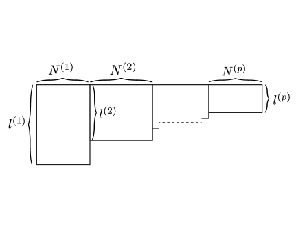
Figure IV.1: We decompose the young diagram corresponding to $\rho$ into $p$ blocks, see III.2.3.

IV.1.2 $T[SU(N)]$

Let us study the large $N$ behavior of our partition functions.

For clarity, let us begin with the $T[SU(N)]$ theories, whose partition function is given in (II.5.51). Let’s rewrite it

$$Z^{T(SU(N))} =(-i)^{\frac{N(N-1)}{2}}\frac{\sum_{w\in\mathfrak{S}_{N}}(-1)^{w}\,e^{2i\pi\sum_{j}^{N}\xi_{j}m_{w(j)}}}{\prod_{j<k}^{N}\textrm{sh}(\xi_{j}-\xi_{k})\textrm{sh}(m_{j}-m_{k})}$$ (IV.1.14)

When the parameters $m_{j}$ and $\xi_{j}$ are generic and kept finite in the limit, we have $\sum_{w\in\mathfrak{S}_{N}}\sim\mathcal{O}(N!)$, whose logarithm contributes $\mathcal{O}(N\ln N)$ to $F_{\rm CFT}$. The remaining contributions come from the two sinh Vandermonde determinants, each of which involves roughly speaking ${N\choose 2}\sim\mathcal{O}(N^{2})$ terms. This gives

$$F_{\rm CFT}\sim\mathcal{O}(N^{2})\ .$$ (IV.1.15)

This is not really surprising since after all our theories are standard gauge theories with gauge group ranks of order $N$.

However, the scaling behavior could change if we consider non-generic values of $m$ and $\xi$. This is exactly happens to our CFT case, where we need to take the limit $m,\xi\to 0$ of (IV.1.14):

$$Z_{\rm CFT}=\lim_{m,\xi\to 0}\big{|}Z_{S^{3}}\big{|}\ .$$ (IV.1.16)

We choose to take the limit in two steps. First, let us take the $\xi\to 0$ limit of (IV.1.14) with $\hat{\rho}=[1,\ldots,1]$. This is conveniently done by setting $\xi=\epsilon w_{N}$ and by taking $\epsilon\to 0$, where $w_{N}$ is defined in (IV.1.12). Using the Weyl denominator formula, we have

$$\sum_{w\in\mathfrak{S}_{N}}(-1)^{w}e^{2\pi i\epsilon w_{N}\cdot m_{\rho}} =\prod_{\alpha>0}2i\sin\left(\pi\epsilon\alpha\cdot m_{\rho}\right)\ =\ \prod_{j<k}2i\sin\left(\pi\epsilon(m_{j}-m_{k})\right)$$

$$\simeq(2i\pi\epsilon)^{\frac{N(N-1}{2}}\prod_{j<k}(m_{j}-m_{k})\ .$$ (IV.1.17)

In the limit $\epsilon_{2}\to 0$, this combines with the factor $\Delta_{\hat{\rho}}(\epsilon w_{N})=\prod_{j<k}2\sinh\pi(\epsilon(j-k))\simeq(2\pi\epsilon)^{\frac{N(N-1}{2}}\prod_{j<k}(j-k)$ in the denominator and the prefactor phase of IV.1.14, giving

$$\left|\prod_{j<k}\frac{1}{(j-k)}\frac{\prod_{j<k}(m_{j}-m_{k})}{\Delta_{\rho}(m)}\right|=\frac{1}{G_{2}(N+1)}\left|\frac{\prod_{j<k}(m_{j}-m_{k})}{\Delta_{\rho}(m)}\right|\ .$$ (IV.1.18)

We next need to take the limit $m\to 0$. This is easy for our case, $\rho=[1,\ldots,1]$;

$$\frac{\prod_{j<k}(m_{j}-m_{k})}{\Delta_{\rho}(m)}=\prod_{j<k}\frac{(m_{j}-m_{k})}{2\sinh\pi(m_{j}-m_{k})}\to(2\pi)^{-\frac{N(N-1)}{2}},$$

which gives

$$Z_{\rm CFT}=\frac{1}{(N-1)!(N-2)!\ldots 2!1!}\left(\frac{1}{2\pi}\right)^{\frac{N(N-1)}{2}}=\frac{1}{G(N+1)}\left(\frac{1}{2\pi}\right)^{\frac{N(N-1)}{2}}\ ,$$ (IV.1.19)

where $G_{2}(x)$ is the Barnes $G$-function defined in Appendix D. From the asymptotics of $G_{2}(x)$ (D.23), we have

$$F_{\rm CFT}=\frac{N^{2}}{2}\ln N+\left[-\frac{3}{4}-\frac{1}{2}\ln\left(\frac{1}{2\pi}\right)\right]N^{2}+\mathcal{O}(N\ln N)\ ,$$ (IV.1.20)

which gives (IV.0.3).

IV.1.3 $T^{\rho}_{\hat{\rho}}[SU(N)]$

Let us consider the more general case given in (IV.0.4).

As long as $\hat{\rho}=[1,\ldots,1]$ the argument of the previous subsection works up until (IV.1.18) with the result for the limit $\xi_{j}\to 0$ given by

$$Z_{\rm CFT} =\frac{1}{G_{2}(N+1)}\left|\frac{\prod_{j<k}(m_{\rho})_{j}-(m_{\rho})_{k}}{\Delta_{\rho}(m_{\rho})}\right|\ .$$ (IV.1.21)

In (IV.1.21) we already have a factor of $G_{2}(N+1)$. Just as in the $T[SU(N)]$ case, this contributes

$$\frac{1}{2}N^{2}\ln N\ ,$$ (IV.1.22)

to the free energy. Next, let us send the mass parameters $m_{j}$ to zero in (IV.1.21). The denominator $\Delta_{\rho}(m)$ goes to zero in the limit, but it can be combined with a subset of the numerator factors given by the $(m_{\rho})_{(a,i,\alpha)}-(m_{\rho})_{(b,j,\alpha)}$ with $a\leq b$, $i<j$, in the notation of IV.1.11 (namely we pick the couples involved in the definition of $\Delta_{\rho}(m)$), yielding a finite answer. We obtain powers of $2\pi$ in this process from the limit of $\Delta_{\rho}(m)$, however this only gives a subleading contribution of order $N^{2}$.

There are still contributions from the numerator $\prod_{j<k}\left[(m_{\rho})_{j}-(m_{\rho})_{k}\right]$, which we have not yet taken into account. In the notation of the previous section the limit of this contribution is

$$(m_{\rho})_{(a,i,\alpha)}-(m_{\rho})_{(b,j,\beta)}=i\left[(w_{l^{(a)}})_{\alpha}-(w_{l^{(b)}})_{\beta}\right]=i(\alpha-\beta)\ ,$$

where $1\leq\alpha\leq l^{(a)},1\leq\beta\leq l^{(b)}$ and $\alpha\neq\beta$.

When the two boxes are in the same block, this contributes a factor

$$\left(N_{5}^{(a)}\right)^{2}\ln\left[(l^{(a)}-1)!(l^{(a)}-2)!\ldots 1!\right]\ ,$$

where the factor $\left(N_{5}^{(a)}\right)^{2}$ accounts for the degeneracy from the column labels $i$. This contributes, under the scaling (IV.0.5),

$$-\frac{1}{2}\left[\kappa_{a}(\lambda^{(a)}\gamma_{a})^{2}\right]N^{2}\ln N+\mathcal{O}(N^{2})\ ,$$ (IV.1.23)

to the free energy. When the two boxes are in the different blocks $a,b$ with $l^{(a)}\geq l^{(b)},\kappa_{a}\geq\kappa_{b}$, the contribution to the free energy is

$$-2\left(N_{5}^{(a)}N_{5}^{(b)}\right)\ln\left[\left(\frac{l^{(a)}+l^{(b)}}{2}-1\right)!\left(\frac{l^{(a)}+l^{(b)}}{2}-2\right)!\ldots\left(\frac{l^{(a)}-l^{(b)}}{2}\right)!\right]\ .$$

The expression inside the bracket gives

$$\ln\left[G_{2}\left(\frac{l^{(a)}+l^{(b)}}{2}+1\right)\right]-\ln\left[G_{2}\left(\frac{l^{(a)}-l^{(b)}}{2}+1\right)\right]\sim\frac{1}{2}l^{(a)}l^{(b)}\ln l^{(a)}\ .$$

Thus the contribution amounts to

$$-2\left(N_{5}^{(a)}N_{5}^{(b)}\right)\frac{1}{2}l^{(a)}l^{(b)}\ln l^{(a)}=-2\frac{1}{2}\left[(\lambda^{(a)}\gamma_{a}\lambda^{(b)}\gamma_{b})\kappa_{a}\right]N^{2}\ln N\ .$$ (IV.1.24)

Collecting all the contributions (IV.1.22), (IV.1.23) and (IV.1.24), we have

$$F_{\rm CFT}=\frac{1}{2}N^{2}\ln N\left[1-\sum_{a=1}^{p}(\lambda^{(a)}\gamma_{a})^{2}\kappa_{a}-2\sum_{a\neq b,\,l^{(a)}>l^{(b)}}(\lambda^{(a)}\gamma_{a}\lambda^{(b)}\gamma_{b})\kappa_{a}\right]+\mathcal{O}(N^{2})\ .$$ (IV.1.25)

From (IV.0.7) we can show that this coincides with (IV.0.8).

In all of the examples above, the leading contribution to the partition function comes from the Barnes $G$-functions. The same $N^{2}\ln N$ type behavior appears in a number of different contexts, such as Gaussian matrix models, $c=1$, topological string on the conifold or more recently in the weak coupling expansion of the ABJM theory [95].

IV.2 Gravity Analysis

In this section we analyze the type IIB supergravity action $S_{\rm gravity}$ on the gravity side. We explain how to regularize the action and provide an explicit formula for any supergravity solution corresponding to linear and circular quiver geometries. Then we evaluate it in the large $N$ limit for the solutions described by the scaling limit IV.0.5. We find perfect agreement with the gauge computations of the previous section.

IV.2.1 The Gravity Action

The type IIB action in Einstein frame is

$$\begin{split}S_{\rm IIB}&=-{1\over 2\kappa_{10}^{2}}\int d^{10}x\sqrt{g}\bigg{\{}R-{4\over 2}\partial_{M}\phi\partial^{M}\phi-\frac{1}{2}e^{4\phi}\partial_{M}\chi\partial^{M}\chi-{1\over 2}e^{-2\phi}|H_{(3)}|^{2}\\ &\qquad-{1\over 2}e^{2\phi}|F_{(3)}+\chi H_{(3)}|^{2}-{1\over 4}|\hat{F}_{(5)}|^{2}\bigg{\}}+{1\over 4\kappa_{10}^{2}}\int d^{10}x\ C_{(4)}\wedge H_{(3)}\wedge F_{(3)}\ ,\end{split}$$ (IV.2.26)

where one imposes the self-duality condition $\hat{F}_{(5)}=*F_{(5)}$ as a supplementary equation. The coupling $\kappa_{10}$ is related to the string scale $\alpha^{\prime}$ by $2\kappa_{10}^{2}=(2\pi)^{7}(\alpha^{\prime})^{4}$.

Due to the presence of the self-duality condition, the action (IV.2.26) cannot be directly used to compute the on-shell value of the action. One way to deal with this is to relax the requirement of Lorentz invariance of the action. In this case an action principle could be obtained along the lines of [96]. As suggested in [97], perhaps the easiest way to implement this for the full type IIB supergravity action is to make a T-duality transformation of the type IIA action. The prescription of [97] (footnote on p.8) consists in reducing $F_{5}$ to its “electric” part (the part along $AdS_{4}$ in our case) and doubling its contribution in the supergravity action. This also corresponds to the alternative non-Lorentz invariant action of [96], which is the true action in a sense, as it need not be supplemented by a self-duality condition.

A simpler method is to first dimensionally reduce the theory to 4-dimensions. After carrying out the dimensional reduction, one can then truncate the theory to the 4-dimensional graviton. To see this is consistent, one may check that the solutions of [21, 22] can be extended by replacing the AdS₄ space with any space which obeys the same Einstein equations. Thus truncating to the 4-dimensional graviton is a consistent truncation.

The effective action for this mode is given by

$$S_{\rm eff}=-\frac{1}{2\kappa_{10}^{2}}{\rm vol}_{6}\int_{\textrm{AdS}_{4}}\!d^{4}x\sqrt{g_{(4)}}(R_{(4)}+6)\ ,$$ (IV.2.27)

where the cosmological constant has been chosen so that the unit AdS₄ space is a solution. The subscript $(4)$ reminds us that $g_{(4)}$ is the 4-dimensional metric and $R_{(4)}$ is the associated Ricci scalar. The quantity ${\rm vol}_{6}$ follows from the initial dimensional reduction and is the volume of the internal space dressed appropriately with the warp factor of AdS₄

$${\rm vol}_{6}=(4\pi)^{2}\int_{\Sigma}d^{2}x(f_{4}f_{1}f_{2})^{2}4\rho^{2}=32(4\pi)^{2}\int_{\Sigma}d^{2}x(-W)h_{1}h_{2}\ .$$ (IV.2.28)

The specific solution we are interested in is AdS₄ with Ricci scalar $R_{(4)}=-12$. Thus the on-shell action becomes simply

$$S_{\rm eff}=-\frac{1}{(2\pi)^{7}(\alpha^{\prime})^{4}}{\rm vol}_{6}\left(\frac{4}{3}\pi^{2}\right)(-6)\ ,$$ (IV.2.29)

where we have used the regularized volume of AdS₄, ${\rm vol}_{AdS_{4}}=(4/3)\pi^{2}$, whose derivation was presented in section I.3 using the method of holographic renormalization.

We emphasize here that the formula IV.2.29 with IV.2.28 provides a remarkably simple exact expression for all the supergravity solutions that describe linear and circular quiver fixed points.

The domain wall solutions (III.2.4), corresponding to defect SCFTs, have a non-compact internal volume, so $vol_{6}$ is infinite and needs further regularization involing (probably) boundary counterterms at $x=\pm\infty$.

IV.2.2 $T[SU(N)]$

Let us first consider the gravity dual for $T[SU(N)]$. The harmonic functions describing the supergravity solution for $\rho=\hat{\rho}=(1,1,...,1)$ (see section III.2.3) are:

$$\begin{split}h_{1}&=-\frac{\alpha^{\prime}N}{4}\ln\bigg{[}\tanh\bigg{(}\frac{i\pi}{4}-\frac{z-\delta}{2}\bigg{)}\bigg{]}+c.c.\ ,\\ h_{2}&=-\frac{\alpha^{\prime}N}{4}\ln\bigg{[}\tanh\bigg{(}\frac{z+\delta}{2}\bigg{)}\bigg{]}+c.c.\ ,\end{split}$$ (IV.2.30)

with

$$\delta=-\frac{1}{2}\ln\left[\tan\left(\frac{\pi}{2N}\right)\right]\ ,$$ (IV.2.31)

where we have used a translation to set $\hat{\delta}=-\delta$. There is one stack of $N$ D5-branes at the position $z=i\frac{\pi}{2}-\frac{1}{2}\ln[\tan(\frac{\pi}{2N})]$ and one stack of $N$ NS5-branes at $z=\frac{1}{2}\ln[\tan(\frac{\pi}{2N})]$ with $N$ D3-branes stretched between them ($N$ units of 5-form flux going from one singularity to the other).

We now wish to take the large $N$ limit of this configuration. It will turn out that locally the Lagrangian density will scale with a factor of $N^{2}$ at leading order in $N$. Secondly, as $N$ goes to infinity, the positions $\delta$ of the 5-brane stacks are sent to infinity in opposite directions (see fig. IV.2). This leaves a large region of geometry between $-\delta$ and $\delta$ of size $\ln N$, which will reproduce the $\ln N$ behavior of the partition function. Thus one can understand the leading behavior of the $T[SU(N)]$ partition function as coming from the geometry located between the two stacks of 5-branes.

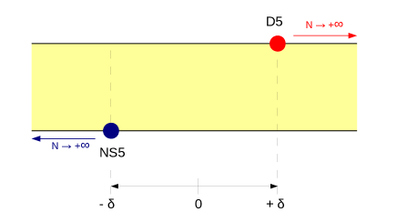
Figure IV.2: Geometry of the $T[SU(N)]$ dual background represented by the strip with two 5-brane singularities at positions $\pm\delta\sim\pm\frac{1}{2}\ln N$. In the large $N$ limit the stacks go to $\pm$ infinity.

To make this more explicit and also compute the exact numerical coefficient, we now work out the large $N$ expansion. First we re-scale the $x$ coordinate so that $z=\delta x+iy$ and then expand the harmonic functions $h_{1}$ and $h_{2}$ around large $N$. At leading order we obtain

$$\begin{aligned} h_{1}&=\alpha^{\prime}\sin(y)N\,e^{\delta(x-1)}+...&&\textrm{if}\ \ x<1\ ,\cr&=\alpha^{\prime}\sin(y)N\,e^{\delta(1-x)}+...&&\textrm{if}\ \ x>1\ ,\cr h_{2}&=\alpha^{\prime}\cos(y)N\,e^{\delta(1+x)}+...&&\textrm{if}\ \ x<-1\ ,\cr&=\alpha^{\prime}\cos(y)N\,e^{-\delta(1+x)}+...&&\textrm{if}\ \ x>-1\ .\end{aligned}$$ (IV.2.32)

From (IV.2.32) we find that the only contribution to the action at this order comes from the central region $-1<x<1$. In this region $W$ is given by $W=-\frac{1}{2}e^{-2\delta}N^{2}(\alpha^{\prime})^{2}\sin(2y)$. Computing the volume of the internal space, (IV.2.28), and plugging into the expression for the effective action, (IV.2.29), we find

$$S_{\rm eff} =\frac{4N^{4}\delta e^{-4\delta}}{\pi^{2}}+...$$ (IV.2.33)

$$=\frac{1}{2}N^{2}\ln N+{\cal O}(N^{2})\ .$$ (IV.2.34)

This reproduces exactly the leading order behavior of the CFT partition function (IV.1.20). Finally we note that including higher order terms in the expansions of the harmonic functions will give additional contributions of order $N^{2}$.

Validity of the computation :

Since we have explicit D5-brane and NS5-brane singularities in the geometry, one may worry about the validity of our approximation. We shall argue that the corrections due to the 5-brane singularities are at most of order $N^{2}$ and do not contribute to the leading $N^{2}\ln N$ behavior. To do so, we first examine the geometry in the central region in the large $N$ limit. The metric factors are given by

$$\begin{aligned} f_{4}^{2}&=\sqrt{2}\alpha^{\prime}Ne^{-\delta}[(2-\cos(2y))(2+\cos(2y))]^{\frac{1}{4}}\ ,\cr f_{1}^{2}&=2\sqrt{2}\alpha^{\prime}Ne^{-\delta}\sin(y)^{2}\left[\frac{2+\cos(2y)}{(2-\cos(2y))^{3}}\right]^{\frac{1}{4}}\ ,\cr f_{2}^{2}&=2\sqrt{2}\alpha^{\prime}Ne^{-\delta}\cos(y)^{2}\left[\frac{2-\cos(2y)}{(2+\cos(2y))^{3}}\right]^{\frac{1}{4}}\ ,\cr 4\rho^{2}&=2\sqrt{2}\alpha^{\prime}Ne^{-\delta}[(2-\cos(2y))(2+\cos(2y))]^{\frac{1}{4}}\ ,\end{aligned}$$ (IV.2.35)

while the dilaton and fluxes are given by (see section III.2.1)

$$\begin{aligned} e^{\phi}&=e^{-\delta x}\left(\frac{2+\cos(2y)}{2-\cos(2y)}\right)^{\frac{1}{4}}\ ,\cr b_{1}&=8\alpha^{\prime}Ne^{-\delta(1+x)}\frac{\sin^{3}(y)}{2-\cos(2y)}\ ,\cr b_{2}&=-8\alpha^{\prime}Ne^{\delta(x-1)}\frac{\cos^{3}(y)}{2+\cos(2y)}\ ,\cr j_{1}&=-e^{-2\delta}N^{2}(\alpha^{\prime})^{2}(3x\delta+\cos(2y))\ .\end{aligned}$$ (IV.2.36)

It is interesting to note that this is exactly the limiting geometry of Janus found in [37] and described by a domain wall solution without 5-brane stacks, so it is simply a domain wall between to $AdS_{5}\times S^{5}$ regions with the same radius but different values for the dilaton. The limit we obtain here looks like the Janus case with an infinite jump in the coupling. The radius $L$ of the Janus space is related to $N$ by $L^{2}=2\sqrt{2}\alpha^{\prime}Ne^{-\delta}$. In the case we consider here, the $\Sigma$ space comes with a natural cutoff at $|x|=\delta$, while for Janus the space is unbounded.

We now consider curvature corrections. Using the above formulas for the metric factor and dilaton, the string frame Ricci scalar in the central region, $-1\leq x\leq 1$, is given by

$$\alpha^{\prime}R =\frac{1}{\pi 2^{1/2}}\bigg{(}\frac{2N}{\pi}\bigg{)}^{\frac{x-1}{2}}\frac{419-60\cos(4y)+\cos(8y)}{(7-\cos(4y))^{2}(2+\cos(2y))^{1/2}}\ .$$ (IV.2.37)

Due to the large $N$ limit, throughout most of the region we have $\alpha^{\prime}R\ll 1$. However, due to the presence of D5-branes, as one approaches $x=1$, $\alpha^{\prime}R$ is of order one and one expects higher curvature corrections to play a role. Since these corrections are localized only in the region near $x=1$, we expect that they do not receive the $\ln N$ enhancement and therefore contribute only at order $N^{2}$. A similar argument can be made when one examines the geometry near the D5-branes using (IV.2.30) before taking the large $N$ limit, showing that the DBI action naively scales like $N^{2}$.

Due to the presence of N5-branes, the second issue for our calculation is to understand if the string coupling, $g_{s}$, is small so that string loop corrections can be ignored. The dilaton in the central region, $-1<x<1$, is given by

$$g_{s}=e^{2\phi} =\bigg{(}\frac{2N}{\pi}\bigg{)}^{-x}\,\sqrt{\frac{2+\cos(2y)}{2-\cos(2y)}}\ .$$ (IV.2.38)

We observe that the dilaton is small in the region $0<x<1$ but is big in the region $-1<x<0$. We first focus our attention on the region $0<x<1$. In the large $N$ limit, the string coupling is small except in the neighborhood of $x=0$, where it is of order one. Thus we expect string loop corrections to be important, but again we argue that since they are localized near $x=0$, they will give contributions at most of order $N^{2}$.

For the region $-1<x<0$, we find that the string coupling is generically large and one might expect string loop corrections to modify the leading $N^{2}\ln N$ behavior. From this point of view, the exact match between gravity and CFT partition functions is surprising and we do not have a good a priori argument for why string loop corrections do not modify the $N^{2}\ln N$ behavior. One possible explanation can be given in terms of a local S-duality transformation in this region. To be more precise, we divide the manifold into three regions $-1<x<-\epsilon$, $-\epsilon<x<\epsilon$ and $\epsilon<x<1$ with $\epsilon\ll 1$. In the first region, we make an S-duality transformation, while in the third region the theory is already weakly coupled. The middle region then has to interpolate between two different S-duality frames and we do not know how to compute the action there. However, since the $\ln N$ enhancement requires the entire internal space and patching only needs to occur locally in the region near $x=0$, one might hope that the middle region does not receive the $\ln N$ enhancement. Of course this argument is only heuristic and it would be interesting to either make it more precise or determine the exact mechanism for why the loop corrections are suppressed.
As for the NS5-branes action, a naive counting of its scaling with $N$, the geometry near the NS5-branes being given by (IV.2.30) before taking the large $N$ limit, leads again to a $N^{2}$ behavior. In the end the justification for all these arguments comes a posteriori from the match with the gauge computation.

IV.2.3 $T^{\rho}_{\hat{\rho}}[SU(N)]$

We now consider more general partitions which take the form (IV.0.4). In this case, there is a single NS5-brane stack and the charge relations, (III.2.36), can be easily inverted to express the phases $\delta_{a}$ and $\hat{\delta}$ in terms of the partitions $\rho$ and $\hat{\rho}$:

$$\delta_{a}-\hat{\delta} =-\ln\left[\tan\left(\frac{\pi}{2}\frac{l^{(a)}}{\hat{N}_{5}}\right)\right]\ .$$ (IV.2.39)

To analyze the large $N$ behavior, we proceed analogously to the $T[SU(N)]$ case and consider the limit where $\hat{\delta}\rightarrow-\infty$ and the $\delta_{a}\rightarrow\infty$. In this case, we approximate the harmonic functions by the following expressions

$$\begin{aligned} h_{1}&=\alpha^{\prime}\sin(y)\sum_{a=1}^{p}N_{5}^{(a)}e^{x-\delta_{a}}+...&&\textrm{if}\ \ x<\delta_{1}\ ,\cr&=\alpha^{\prime}\sin(y)\sum_{a=i}^{p}N_{5}^{(a)}e^{x-\delta_{a}}+...&&\textrm{if}\ \ \delta_{i}<x<\delta_{i+1}\ ,\cr h_{2}&=\alpha^{\prime}\cos(y)\hat{N}_{5}e^{-(x-\hat{\delta})}+...&&\textrm{if}\ \ x>\hat{\delta}\ ,\end{aligned}$$ (IV.2.40)

while the regions with $x>\delta_{p}$ and $x<\hat{\delta}$ will give only subleading contributions. In this approximation we find that $W=-h_{1}h_{2}$ so that

$$\begin{aligned} -Wh_{1}h_{2}&=\frac{1}{4}(\alpha^{\prime})^{4}\hat{N}_{5}^{2}\left(\sum_{a=1}^{p}N_{5}^{(a)}e^{-(\delta_{a}-\hat{\delta})}\right)^{2}\sin^{2}(2y)&&\textrm{if}\ \ \hat{\delta}<x<\delta_{1}\ ,\cr&=\frac{1}{4}(\alpha^{\prime})^{4}\hat{N}_{5}^{2}\left(\sum_{a=i}^{p}N_{5}^{(a)}e^{-(\delta_{a}-\hat{\delta})}\right)^{2}\sin^{2}(2y)&&\textrm{if}\ \ \delta_{i}<x<\delta_{i+1}\ .\end{aligned}$$ (IV.2.41)

Using this in (IV.2.28) we find

$$\textrm{vol}_{6} =32(4\pi)^{2}\int_{\hat{\delta}}^{\delta_{p}}\!dx\int_{0}^{\frac{\pi}{2}}\!dy\,(-Wh_{1}h_{2})$$

$$=32\pi^{3}(\alpha^{\prime})^{4}\hat{N}_{5}^{2}\sum_{i=1}^{p}\left(\sum_{a=i}^{p}N_{5}^{(a)}e^{-(\delta_{a}-\hat{\delta})}\right)^{2}(\delta_{i}-\delta_{i-1})$$ (IV.2.42)

where we define $\delta_{0}\equiv\hat{\delta}$. Plugging into (IV.2.29) and combining all of the numerical factors, we obtain

$$S_{\rm eff} =\frac{2}{\pi^{2}}\hat{N}_{5}^{2}\sum_{i=1}^{p}\left(\sum_{a=i}^{p}N_{5}^{(a)}e^{-(\delta_{a}-\hat{\delta})}\right)^{2}(\delta_{i}-\delta_{i-1})+...\ .$$ (IV.2.43)

We now consider the scaling behavior defined by (IV.0.5), which introduces separations between the $\delta_{a}$ which are of order $\ln N$. In this case each region between a given $\delta_{a}$ and $\delta_{a+1}$ will contribute to the action at order $N^{2}\ln N$. In terms of this scaling the action becomes

$$S_{\rm eff} =\frac{1}{2}N^{2}\left[\left(\sum_{a=1}^{p}\gamma_{a}\lambda^{(a)}\right)^{2}\ln\left(\frac{2}{\pi}\frac{\hat{\gamma}}{l^{(1)}}N\right)+\sum_{i=2}^{p}\left(\sum_{a=i}^{p}\gamma_{a}\lambda^{(a)}\right)^{2}\ln\left(\frac{l^{(i-1)}}{l^{(i)}}\right)\right]+{\cal O}(N^{2})\ ,$$

$$=\frac{1}{2}N^{2}\ln N\left[(1-\kappa_{1})+\sum_{i=2}^{p}\left(\sum_{a=i}^{p}\gamma_{a}\lambda^{(a)}\right)^{2}\left(\kappa_{i-1}-\kappa_{i}\right)\right]+{\cal O}(N^{2})\ ,$$ (IV.2.44)

which coincides with (IV.0.8).

Computing the $N$ dependence of the metric and dilaton we find here $g_{\mu\nu}\sim N^{2}$ and $e^{2\phi}\sim N^{\kappa_{1}}$. This implies that the curvature is small everywhere (except in the close vicinity of the D5-branes) as in the $T[SU(N)]$ case, but now the dilaton is very large on the whole region between the 5-branes. This is different from the $T[SU(N)]$ case. Now our computation is justified, because we can use S-duality to dualize to obtain a solution with small $e^{2\phi}$ everywhere. This is in agreement with our analysis of §III.4.3.

IV.2.4 Subleading Terms

So far we have concentrated on the leading $N^{2}\ln N$ contributions to the free energy and it is a natural question to ask about the subleading $N^{2}$ contributions. Comparing the CFT and gravity partition functions, we find that the subleading $N^{2}$ contributions do not match. However, this is not surprising since the gravity solution contains 5-brane singularities around which supergravity approximation breaks down. Additionally, as already mentioned, there are regions in the bulk of $\Sigma$ where the string coupling becomes large. It would be interesting to interpret and if possible match the subleading contributions to the CFT partition function with higher curvature corrections, coming from both string and loop corrections, on the gravity side. For the $T[SU(N)]$ theory, we note that near the D5-brane singularity, the Ricci scalar, (IV.2.37) does not depend on $N$ and so all powers of $R$ will contribute at order $N^{2}$. Similarly, one may check that other contractions of the Riemann tensor will also contribute at order $N^{2}$. Thus even at order $N^{2}$, the CFT partition function contains information about all orders of the higher curvature corrections.

IV.3 Consistency with F-theorem

The results IV.0.8 we have found for the free energy of $T^{\rho}_{\hat{\rho}}[SU(N)]$ SCFTs in the large $N$ limit obey the inequality

$$F_{T^{\rho}_{\hat{\rho}}[SU(N)]}\leq F_{T[SU(N)]}\ .$$ (IV.3.45)

Our results suggest that this inequality is true for any $T^{\rho}_{\hat{\rho}}[SU(N)]$ SCFTs.

This is to be compared with the hypothetic F-theorem ([34, 98, 99, 100, 101]), whose weaker version stipulates that when two SCFTs are connected by a RG flow the free energy of the UV theory is bigger than the free energy of the IR theory $F_{UV}\geq F_{IR}$. A stronger version was formulated in [99] where the free energy was defined along the RG-flow and the proposed F-theorem says that it is monotonicaly decreasing along the flow. A relation of proportionality between the free energy on the 3-sphere and a certain entanglement entropy was shown in [102] and used in [103] to argue for the F-theorem. Non-supersymmetric examples have also been studied [100]. The F-theorem would be the analogue of the $c$-theorem in 2 dimensions ([104]) and $a$-theorem in 4 dimensions ([105]).

It is actually possible to argue that IV.3.45 is a manifestation of the F-theorem. To show it we have to find a deformation of the $T[SU(N)]$ SCFT initiating a flow to an arbitrary $T^{\rho}_{\hat{\rho}}[SU(N)]$ SCFT.

The deformations that we need to consider can be understood from the brane picture. Let’s consider the brane picture associated to the quiver of $T[SU(N)]$, shown in figure IV.3 for $N=4$. We can modify the partition $\hat{\rho}=(1,1,...,1)$ to any partition $\hat{\rho}^{\prime}$ by separating D3-segments connecting NS5-branes in transverse space (along $x^{4},x^{5},x^{6}$) (see figure IV.3) and let the theory flow to the IR. The IR SCFT resulting from this flow should be composed of decoupled pieces : the SCFT $T^{(1,1,..,1)}_{\hat{\rho}^{\prime}}[SU(N)]$ and a number of decoupled $U(1)$ vector multiplets corresponding to the separated D3-segments.

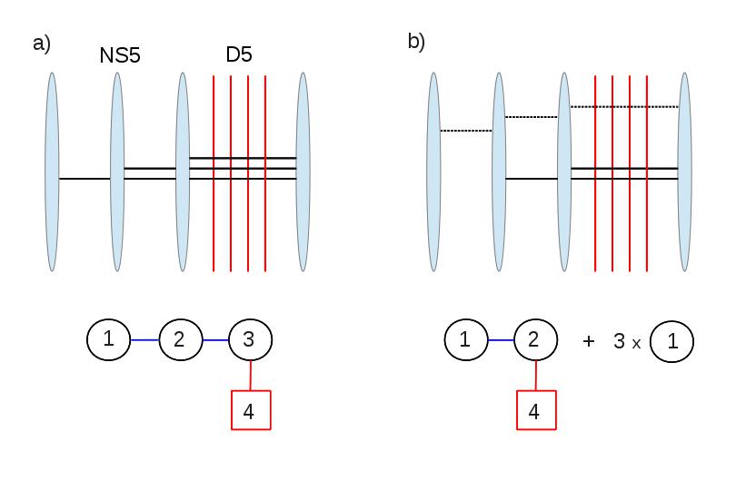
Figure IV.3: a) Brane picture and quiver for $T[SU(4)]$ SCFT. b) After separating 3 D3-segments in transverse space (doted segments) the theory flow to the SCFT described by $\hat{\rho}^{\prime}=(2,1,1)$ plus 3 decoupling abelian vector multiplets, as described by the quiver below the figure.

In gauge theory the brane manipulation that consists in moving a D3-segment in transverse space corresponds to moving on the Coulomb branch of vacua. So the RG-flow that we are looking for is initiated by giving vevs to the scalars in the vector multiplets.

Let’s consider the minimal example of separating one D3-segment in a $T^{\rho}_{\hat{\rho}}[SU(N)]$ SCFT with

$$\rho =(l_{1},l_{2},...,l_{k})$$

$$\hat{\rho} =(\hat{l}_{1},\hat{l}_{2},...,\hat{l}_{\hat{k}}).$$ (IV.3.46)

Separating a D3-segment from the $N_{J}$ segments of the $J$-th node $U(N_{J})$ amounts to giving a vev to the scalars in the vector multiplet of this node, so that the gauge symmetry is broken to $U(N_{J}-1)\times U(1)$. If the (adjoint) scalars are represented by $N_{J}\times N_{J}$ matrices, this means giving a vev to a corner element of the matrices. When flowing to the infrared, the $U(N_{J})$ gauge symmetry is higgsed to $U(N_{J}-1)\times U(1)$. The $U(1)$ vector multiplet decouples from the matter fields (as it was coupled only through massive modes), so we end up with the SCFT $T^{(1)}_{\hat{\rho}^{\prime}}[SU(N)]$ which is the same as $T^{\rho}_{\hat{\rho}}[SU(N)]$ except that the node $U(N_{J})$ is replaced by $U(N_{J}-1)$, plus a free $U(1)$ vector multiplet.
The new partition $\hat{\rho}^{\prime}$ is given by

$$\hat{\rho}^{\prime}=\left(\hat{l}_{1}\,,\,...\,,\,\hat{l}_{J-1}\,,\,\hat{l}_{J}+1\,,\,\hat{l}_{J+1}-1\,,\,\hat{l}_{J+2}\,,\,...\,,\,\hat{l}_{\hat{k}}\right)\ .$$ (IV.3.47)

The new partition $\hat{\rho}^{\prime}$ may not be ordered, in which case the IR SCFT is not irreducible and is believed to flow to the IR irreducible fixed point of the theory with ordered partition, plus decoupling hypermultiplets, as explained in section II.2. The hypermultiplets in question are actually twisted hypermultiplets (transformation properties under $SU(2)_{L}\times SU(2)_{R}$ interchanged) that are exactly the $U(1)$ vector multiplets that we just saw. Actually the reordering of the NS5-branes, which is the reordering of the partition $\rho^{\prime}$, can be effectively done by separating more D3-segments from the brane configuration (moving the Coulomb branch of other nodes) and flowing to the infrared. In the process we obtain again decoupled $U(1)$ vector multiplets, but in 3-dimension abelian vector multiplets can be dualized to twisted hypermultiplets (see §II.1), through the relation $F_{\mu\nu}=\epsilon_{\mu\nu\sigma}\partial^{\sigma}\gamma$, where $\gamma$ is a real scalar named dual photon. The decoupling of abelian vector multiplets is thus the decoupling of the twisted hypermultiplets of [11].

The dual minimal example consists in moving a D3-segment that is stretched between two D5-branes. For instance let’s consider the case of $M_{J}$ D5-branes intersecting the $N_{J}$ D3-segments of the $J$-th node and we move a D3-segment stretched between two D5-branes, as shown in figure IV.4 (we assume $M_{J}\geq 2$). From our understanding of mirror symmetry, which exchanges the Coulomb branch and the Higgs branch of the theories, we guess that the correct flow will be initiated this time by moving on the Higgs branch of the theory. The brane situation that we have described corresponds to having a $U(N_{J})$ gauge node with $M_{J}$ fundamental hypermultiplets. Let’s consider the scalars in two hypermultiplets (2 complex in each). They can be combined in a couple of complex matrices $A,\tilde{A}$ of size $N_{J}\times 2$ and $2\times N_{J}$ respectively, where $A$, resp. $\tilde{A}$, contains the scalars transforming in the fundamental, resp. anti-fundamental, representation of $U(N_{J})$. Setting to zero the vevs of the other fundamental hypermultiplets and possible bifundamental hypermultiplets, the matrices $A$ and $\tilde{A}$ have to satisfy the constraints $A\tilde{A}=0$ (critical point of the superpotential) and $AA^{\dagger}-\tilde{A}^{\dagger}\tilde{A}=0$ (D-term). Preserving these constraints we may move on the Higgs branch by turning on constant vevs $a$ and $-a$ for the first row of $A$ and the first column of $\tilde{A}$ :

$$A=\begin{bmatrix}a&a\\ 0&0\\ ..&..\\ 0&0\end{bmatrix}\quad,\quad\tilde{A}=\begin{bmatrix}a&0&...&0\\ -a&0&...&0\end{bmatrix}$$ (IV.3.48)

The $U(N_{J})$ gauge transformations act by left multiplication on $A$ and right multiplication on $\tilde{A}$, so at this point on the Higgs branch the gauge group is broken to $U(N_{J}-1)$. From the massless degrees of freedom of the $M_{J}$ hypermultiplets, some are eaten in the process and some decouple from the quiver theory (in the infrared). In total there are $M_{J}-1$ decoupling hypermultiplets. In the infrared the gauge group is thus higgsed to $U(N_{J}-1)$, with $M_{J}-2$ hypermultiplets in the fundamental representation. The bifundamental hypermultiplet in $U(N_{J-1})\times U(N_{J})$, resp. $U(N_{J})\times U(N_{J+1})$, splits into a bifundamental of $U(N_{J-1})\times U(N_{J}-1)$, resp. $U(N_{J}-1)\times U(N_{J+1})$, plus a fundamental hypermultiplet in $U(N_{J-1})$, resp. $U(N_{J+1})$.
This is in complete agreement with the brane picture : moving a D3-segment between to D5-branes to infinity and displacing the D5-branes so that the net number of D3-brane ending on them is zero (one D5 moves to the node on the left, while the other D5 moves to the node on the right), we get a brane picture corresponding to the quiver theory we just described (see figure IV.4). There are $M_{J}-1$ decoupling hypermultiplets corresponding to the D3-segment (that we moved away) splitting in $M_{J}-1$ D3-segments inbetween the $M_{J}$ D5-branes.

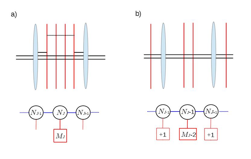
Figure IV.4: a) Brane picture corresponding to moving a D3-segment stretched bewteen two D5-branes. b) Final brane configuration after moving the D5-branes (and D3 segment at infinity) and corresponding quiver gauge theory.

The partition $\rho^{\prime}$ obtained for the infrared linear quiver is

$$\rho^{\prime}=\big{(}...\ ,\ \overbrace{l^{(J)}+1\ ,\ l^{(J)}\ ,\ ...\ ,\ l^{(J)}\ ,l^{(J)}-1}^{N^{(J)}_{5}}\ ,\ ...\big{)}\ ,$$ (IV.3.49)

which corresponds to the minimal case for moving on the Higgs branch.

This shows that, by moving on the Coulomb branch and Higgs branch, we can flow from $T[SU(N)]$ to any $T^{\rho}_{\hat{\rho}}[SU(N)]$ SCFT plus decoupling hypermultiplets. The F-theorem then predicts

$$F_{T[SU(N)]}\ \geq\ F_{T^{\rho}_{\hat{\rho}}[SU(N)]}\,+\,F_{hypers}\ >\ F_{T^{\rho}_{\hat{\rho}}[SU(N)]}\ ,$$

where the second inequality follows from the fact that the free energy of a free hypermultiplet (computed via localization techniques on the 3-sphere [15]) is $\frac{1}{2}$.

This prediction is confirmed by our results IV.3.45.

One may wonder if it is possible to derive inequalities comparing the free energy of to arbitrary SCFTs $T^{\rho_{1}}_{\hat{\rho}_{1}}[SU(N)]$ and $T^{\rho_{2}}_{\hat{\rho}_{2}}[SU(N)]$. Reasoning along the same lines (D3-segments decoupling) one can understand that we cannot derive inequalities for any two such SCFTs but only in some cases :

$$\left\{\begin{array}[]{c}\rho_{1}\geq\rho_{2}\\ \hat{\rho}_{1}\geq\hat{\rho}_{2}\end{array}\right.\quad\Longrightarrow\quad F_{T^{\rho_{1}}_{\hat{\rho}_{1}}[SU(N)]}\leq F_{T^{\rho_{2}}_{\hat{\rho}_{2}}[SU(N)]}\ .$$ (IV.3.52)

An easy way to derive this inequality is to consider the brane configuration corresponding to a quiver when the 5-branes are separated (NS5-branes on the left, D5-branes on the right, II.4). In this brane configuration the partitions of $N$ are directly visible with the D3-branes ending on the 5-branes. The inequality $\hat{\rho}_{1}\geq\hat{\rho}_{2}$ means that we can transform $\hat{\rho}_{2}$ into $\hat{\rho}_{1}$ by decoupling D3-segments stretched between NS5-branes from the brane configuration of $T^{\rho_{2}}_{\hat{\rho}_{2}}[SU(N)]$. Similarly, if $\rho_{1}\geq\rho_{2}$ we can transform $\rho_{2}$ into $\rho_{1}$ by decoupling D3-segments stretched beween D5-branes. Decoupling the D3-segments as indicated, one is left with the brane configuration of $T^{\rho_{1}}_{\hat{\rho}_{1}}[SU(N)]$ leading to the inequality IV.3.52.

The result that was found for the free energy IV.0.8 confirms the prediction IV.3.52 from the F-theorem in simple cases : let’s consider two theories of the form IV.0.4, IV.0.5, with $\rho_{1}=\rho_{2}$, identical parameters $\gamma_{a},\lambda^{(a)}$ but different scalings $\kappa_{a}^{(1)}$ $\kappa_{a}^{(2)}$. Imposing $\kappa_{a}^{(1)}\geq\kappa_{a}^{(2)}$ for all $a$ ensures that $\hat{\rho}_{1}\geq\hat{\rho}_{2}$. In this case we have $F_{T^{\rho_{1}}_{\hat{\rho}_{1}}[SU(N)]}\leq F_{T^{\rho_{2}}_{\hat{\rho}_{2}}[SU(N)]}$ because the coefficient in front of each $\kappa_{a}$ in IV.0.8 is negative.

It would be interesting to see if IV.3.52 can be checked on the supergravity side using the general formula IV.2.29 at finite $N$. This is not really expected to work since the supergravity regime is at large $N$, but it might be that the regularized on-shell supergravity action is a protected quantity, as our computations tend to suggest.

Chapter V Solutions with $(p,q)$-5branes and Chern-Simons SCFTs

Classical type-IIB supergravity has a continuous global $SL(2,\mathbb{R})$ symmetry [106] which transforms the axion-dilaton field, $S=\chi+ie^{-2\phi}$, and the NS-NS and R-R three-form field strengths as follows:

$$S^{\prime}={aS+b\over cS+d}\ ,\qquad\left(\begin{array}[]{c}\,\,H_{(3)}^{\prime}\\ F_{(3)}^{\prime}\end{array}\right)=\left(\begin{array}[]{cc}d&-c\\ -b&a\end{array}\right)\left(\begin{array}[]{c}\,H_{(3)}\\ F_{(3)}\end{array}\right)\ ,$$ (V.0.7)

where $a,b,c,d$ are real numbers with $ad-bc=1$. The transformations leave invariant the Einstein-frame metric, and the gauge-invariant five-form field strength.

As is well known, only the integer subgroup $SL(2,\mathbb{Z})$ is a symmetry of the full string theory [107], whereas continuous transformations can be used to generate inequivalent solutions. The authors of [21] have indeed used such $SL(2,\mathbb{R})$ transformations to bring the general solution of the Killing-spinor equations to the local form given in §III.2.1. Conversely, acting with the transformations (V.0.7) generates new solutions from the ones of section 3, with singularities that correspond to general $(p,q)$ five-branes. We will now discuss briefly these new solutions. In this section we focus on the solutions on the annulus, however the discussion is directly applicable to the solutions on the strip (linear quiver solutions or defect solutions).

V.1 Solutions with $(p,q)$ five-branes

The solutions given by the harmonic functions (III.2.34) or (III.3.57) have singularities on the upper boundary of the infinite strip or the annulus that correspond to D5-branes, and singularities on the lower boundary that correspond to NS5-branes. The charges are, respectively, $\gamma^{(e)}$ and $\hat{\gamma}^{(f)}$ for the stacks labeled by $e$ and $f$. Since the metric is invariant, the $SL(2,\mathbb{R})$ transformations do not change the positions and the total number of five-brane stacks. It transforms, however, their charges as follows

$$\gamma^{(e)}(0,1)\to\gamma^{(e)}(-c,a)\qquad{\rm and}\qquad\hat{\gamma}^{(f)}(1,0)\to\hat{\gamma}^{(f)}(d,-b)\ ,$$ (V.1.8)

where the NS5-brane and D5-brane charges are arranged as usual in a doublet. Let us write $(-c,a)=w(p,q)$ and $(d,-b)=\hat{w}(\hat{p},\hat{q})$, where $p,q$ and $\hat{p},\hat{q}$ are pairs of relatively-prime integers. Charge quantization requires that

$$N_{5}^{(e)\,\prime}=w\gamma^{(e)}\quad{\rm and}\quad\hat{N}_{5}^{(f)\,\prime}=\hat{w}\hat{\gamma}^{(f)}$$ (V.1.9)

be integer for all $e$ and $f$. Since the $\gamma$’s and $\hat{\gamma}$’s are arbitrary parameters, this can always be arranged to get any desired number of five-branes in each stack. The only conditions are that all five-branes on the upper boundary are of the same kind, including the sign, that the same is true for all five-branes on the lower boundary, and that furthermore these two kinds are different, $p\hat{q}-q\hat{p}\not=0$. This last constraint follows from the fact that the $SL(2,\mathbb{R})$ matrix has determinant one.

It should be stressed that the $SL(2,\mathbb{R})$ transformations take us, in general, outside the ansatz of §III.2.1; they generate in particular a non-vanishing R-R axion field. The only exception is S-duality ($S\to-1/S$) which interchanges the harmonic functions, and acts as mirror symmetry on the holographically-dual SCFT.

Consider next the D3-brane charges. These are not affected by $SL(2,\mathbb{R})$ transformations, provided one transforms the gauge choice covariantly. More explicitly, let us consider the D3-brane charge of the $(p,q)$ singularities in the upper boundary. The 2-form that has no component on $S_{2}^{2}$ [and is therefore well defined on a patch containing the whole upper boundary where this 2-sphere shrinks] is $B_{(2)}=aB_{(2)}^{\prime}+cC_{(2)}^{\prime}$. The D3-brane charge of a $(p,q)$ five-brane stack is given therefore by the integral of the following closed five-form

$$N_{3}^{(e)\,\prime}={1\over(4\pi\alpha^{\prime})^{2}}\int_{{\cal C}_{e}^{5}}\left[F_{(5)}-(aB_{(2)}^{\prime}+cC_{(2)}^{\prime})\wedge(bH_{(3)}^{\prime}+dF_{(3)}^{\prime})\right]\ ,$$ (V.1.10)

with the gauge choice $aB_{(2)}^{\prime}+cC_{(2)}^{\prime}=0$ in the lower-boundary segment $[\hat{\delta}_{1},2t]$. This is identical to the integral in the non-transformed solution, so that , in the case of the annulus solutions for instance,

$$N_{3}^{(e)\,\prime}=\gamma_{e}\sum_{f=1}^{\hat{p}}\hat{\gamma}_{f}\,\left(-\frac{i}{2\pi}\ln\bigg{[}\frac{\vartheta_{1}\left(\nu_{ef}|\tau\right)}{\vartheta_{1}\left(\bar{\nu}_{ef}|\tau\right)}\frac{\vartheta_{2}\left(\bar{\nu}_{ef}|\tau\right)}{\vartheta_{2}\left(\nu_{ef}|\tau\right)}\bigg{]}-\frac{4}{\pi\alpha^{\prime}}\varphi_{2}\right)\ ,$$ (V.1.11)

which is the same result as (III.3.66). The quantization of this charge puts the same constraints on the continuous parameters as in the untransformed solution. This is not however the case for the quantization of individual linking numbers, since the number $w\gamma^{(e)}$ of $(p,q)$ five-branes depends, via $w$, on the $SL(2,\mathbb{R})$ transformation.

Among all the solutions discussed here, those related by $SL(2,\mathbb{Z})$ transformations are physically equivalent [107]. To characterize inequivalent solutions, we may perform a $SL(2,\mathbb{Z})$ transformation that maps $(\hat{p},\hat{q})$ to $(1,0)$, so that the singularities on the lower boundary correspond to pure NS5-branes. Using then the shift symmetry $(p,q)\to(p+ql,q)$, which leaves invariant the NS5 branes, we can bring the second type of five-branes to a canonical form $(p,q)$ with $0\leq p<|q|$ (see figure V.1).

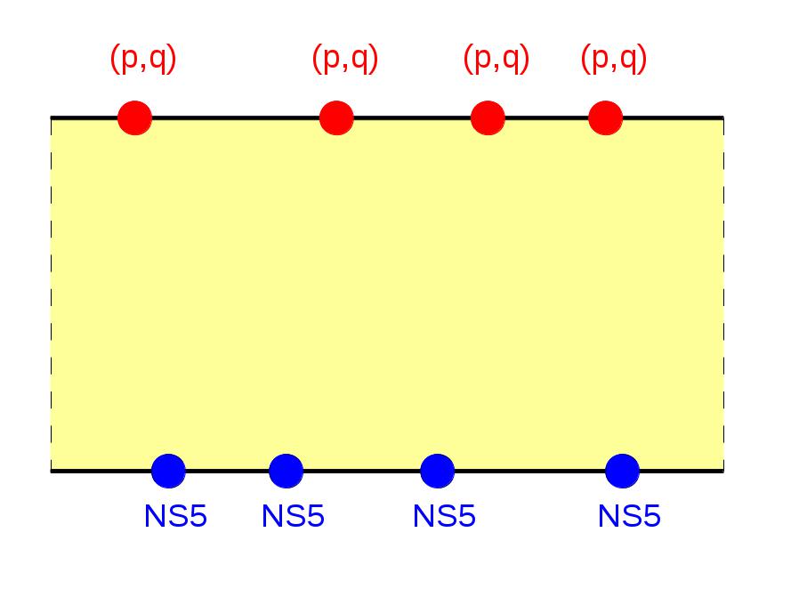
Figure V.1: Canonical solution on the annulus with NS5-branes on the lower boundary and $(p,q)$-5branes on the upper boundary, $0\leq p<|q|$.

The $SL(2,\mathbb{R})$ transformation from the ansatz of §III.2.1 to the above canonical form of the general solution is effected by the following matrix

$$\left(\begin{array}[]{cc}\hat{w}&-wp\\ 0&wq\end{array}\right)\quad{\rm with}\quad w\hat{w}q=1\ .$$ (V.1.14)

Multiplying (V.1.11) with $w\hat{w}q$, using (V.1.9) and the infinite-product expressions for the $\vartheta$-functions gives

$${N^{(a)\,\prime}_{3}}=qN^{(a)\,\prime}_{5}\sum_{b=1}^{\hat{p}}\hat{N}^{(b)\,\prime}_{5}\Big{[}\sum_{n=0}^{+\infty}f(\hat{\delta}_{b}-\delta_{a}-2nt)-\sum_{n=1}^{+\infty}f(-\hat{\delta}_{b}+\delta_{a}-2nt)\Big{]}\ ,$$ (V.1.15)

and likewise

$${\hat{N}^{(b)\,\prime}_{3}}=q\hat{N}^{(b)\,\prime}_{5}\sum_{a=1}^{p}N^{(a)\,\prime}_{5}\Big{[}\sum_{n=1}^{+\infty}f(-\hat{\delta}_{b}+\delta_{a}-2nt)-\sum_{n=0}^{+\infty}f(\hat{\delta}_{b}-\delta_{a}-2nt)\Big{]}\ .$$ (V.1.16)

A similar expression can be written for the winding charge $L^{\prime}$. Integrality of the linking numbers, $l^{\prime}_{a}=N^{(a)\,\prime}_{3}/N^{(a)\,\prime}_{5}$ and $\hat{l}^{\prime}_{b}=\hat{N}^{(b)\,\prime}_{3}/\hat{N}^{(b)\,\prime}_{5}$, constraints the positions of the singularities on the boundary of $\Sigma$ and the modulus $t$ (in the case of the annulus). When $q\not=1$ there are more inequivalent allowed solutions than in the case of pure D5-branes and NS5-branes, corresponding to different choices of $p$, with $0\leq p<|q|$.

The charges (V.1.15) and (V.1.16) obey the sum rule (III.3.72), and they thus still define two partitions $\rho$ and $\hat{\rho}$ of some integer $N$.
To summarize, the inequivalent solutions are classified by the two partitions $\rho,\hat{\rho}$, the winding charge $L$ and the type of 5-branes on the upper boundary ($(p,q)$-5branes with $0\leq p<|q|$).

Furthermore, these partitions still satisfy the basic inequalities $L+\rho^{T}>\hat{\rho}$ (II.3.36). In general, we have no clear argument for why these conditions should be obeyed on the gauge-theory side. Indeed, for arbitrary $(p,q)$ there is no known Lagrangian description of the field theory (we refer the reader to section 8 of [11] for more details). Such a description only exists for the configurations involving $(1,k)$ 5-branes [14, 20, 86] : the $U(N)$ gauge theory living on a stack of $N$ D3-branes has level $k$ or $-k$ Chern-Simons terms depending on whether the D3-branes end on the $(1,k)$ five-brane from the left or the right.

V.1.1 IIB dual of ABJM gauge theory

The famoust example of such Chern-Simons SCFT is the ABJM theory presented at the end of section I.2. The gauge theory is of circular type, with Chern-Simons gauge group $U(N)_{M}\times U(N)_{-M}$ and two bifundamental hypermultiplets. The indices $M$ and $-M$ refer to the Chern-Simons levels of the two gauge factors. The corresponding brane configuration was pictured in figure I.2 for the more general ABJ theory (nodes of different ranks).

Let’s describe the IIB dual solutions of ABJM as an example.
The data of the ABJM theory are the type of 5-brane on the upper boundary, which is the $(1,M)$ 5-brane, the number $N$ of winding D3-brane charge and the two partitions (with a single entry) $\rho=\hat{\rho}=[0]$, reflecting the fact that in the brane confiration no D3-branes end on the 5-branes. Here we took a liberty with our description of circular quivers, which are supposed to have positive linking numbers. The correct partitions are obtained after a Hanny-Witten move (winding of one 5-brane around the circle), which creates $M$ D3-branes stretched between the NS5 and the $(1,M)$ 5-brane, and are given by $\rho=\hat{\rho}=[M]$ . Our non-standard choice of partitions corresponds to the same quiver theory and will be described by the same supergravity solution, but with a different gauge fixing (see section III.3.3 for details).

To find the supergravity solution we need to understand the $SL(2,\mathbb{R})$-related solution with vanishing axion field, then give the associated harmonic functions $h_{1},h_{2}$ and implement the $SL(2,\mathbb{R})$-tranformation.

The $SL(2,\mathbb{R})$-related solution with vanishing axion field is the solution with $N$ winding D3-branes, one NS5-brane and one stack of $M$ D5-branes. The non-standard partitions are $\hat{\rho}=[0]$ and $\rho=[0,0,...,0]$ ($M$ entries).
The parameters of the IIB solution are the period $t$ of the annulus and the distance $\Delta=\hat{\delta}-\delta$ on the $x$ axis between the D5 and NS5-branes. They are determined by the equations (III.3.2,III.3.70) for the charges

$$N =M\sum_{n=1}^{\infty}n\Big{[}f(\Delta-2nt)+f(-\Delta-2nt)\Big{]}$$

$$0 =M\Big{[}\sum_{n=1}^{+\infty}f(-\Delta-2nt)-\sum_{n=0}^{+\infty}f(\Delta-2nt)\ ,\Big{]}$$ (V.1.17)

with $f(x)=(2/\pi)\arctan(e^{x})$. The second equation express the D3-charge of the NS5-brane or equivalently the D3-charge of the D5-branes. It is solved for the $\Delta=-t$ and the parameter $t$ is fixed by the first equation, which (unfortunately) is not easily inverted.

$$\Delta=-t\quad,\quad N=M\,\sum_{n=0}^{\infty}(2n+1)\,f\big{[}-(2n+1)t\big{]}\ .$$ (V.1.18)

Setting $\hat{\delta}=0$, the harmonic functions describing the solution are (III.3.57)

$$h_{1} =-M\ \ln\bigg{[}\frac{\vartheta_{1}\left(\nu|\tau\right)}{\vartheta_{2}\left(\nu|\tau\right)}\bigg{]}+c.c.\ ,\ \qquad{\rm with}\ \ \ i\,\nu=-\frac{z-t}{2\pi}+\frac{i}{4}\ ,\ \tau=it/\pi\ ,$$ (V.1.19)

$$h_{2} =\ -\ \ln\bigg{[}\frac{\vartheta_{1}\left(\hat{\nu}|\tau\right)}{\vartheta_{2}\left(\hat{\nu}|\tau\right)}\bigg{]}+c.c.\ ,\ \ \qquad{\rm with}\ \ \ i\,\hat{\nu}=\frac{z}{2\pi}\ .$$ (V.1.20)

If we parametrize the $x$-axis of the annulus by $-t\leq x\leq t$, the free constants in the holomorphic functions $\mathcal{A}_{1},\mathcal{A}_{2}$ III.3.59 are fixed so that $B_{2}=0$ on the lower boundary $(0,t]$ and $C_{2}=0$ on the upper boundary $[-t,t)$.

The supergravity solution given by V.1.19 describe the metric and 5-form of the IIB dual of ABJM. The dillaton and 3-forms are obtained by acting with the $SL(2,\mathbb{R})$ transformation

$$\left(\begin{array}[]{cc}1&M^{-1}\\ 0&1\end{array}\right)\ .$$ (V.1.23)

In terms of the axion-dilaton $S=ie^{-2\phi}$ and the 3-forms $H_{3},F_{3}$ of the (vanishing axion) solution V.1.19, we get, using V.0.7,

$$S^{\prime}=\frac{M}{1+M^{2}\,e^{4\phi}}\big{(}-1+iM\,e^{2\phi}\big{)}\ ,\qquad H^{\prime}_{3}=H_{3}+\frac{1}{M}\,F_{3}\ ,\ F^{\prime}_{3}=F_{3}\ .$$ (V.1.24)

It is nessecary to pause here to comment about the solution we found. The metric is given in terms of the harmonic functions V.1.19 and it is way more complicated than the ABJM type IIA or M-theory metrics I.2.15, I.2.14. When going from type IIA to type IIB using T-duality (see appendix C) one end up with the smeared solution that we got in the large $N$ ($L$) limit in §III.4.2, which is indeed much more simple.
This reveals that the ususal rules for T-duality are not enough to get the full type IIB solution. Even the simpler problem of T-dualizing pure NS5-branes is notoriously subtle [93, 31, 94, 108]. As explained in these references, the contributions of world-sheet instantons are responsible for the localization of the NS5-branes on the type-IIB side [31], and for creating the dual throats in winding space on the type-IIA side [94]. The correct T-dual backgrounds have localized singularities, breaking the invariance under translation along the annulus, and encodes the full data $(\rho,\hat{\rho},L)$ describing the quiver theory. It would be very interesting to understand this T-duality precisely and to be able to relate the corrections to the metric (compared to the smeared case) to dual quantities in type IIA string theory and M-theory.

Comment about supersymmetry and brane configurations

In the above description we considered brane configurations with $(1,k)$-5branes orthogonal to NS5-branes. Such brane configurations preserve $\mathcal{N}=4$ supersymmetry in 3-dimensions. However it is known that Yang-Mills Chern-Simons gauge theories in 3-dimensions have only up to $\mathcal{N}=3$ supersymmetry, and the brane configuration preserving $\mathcal{N}=3$ has the $(1,k)$-5brane and the NS5-brane at an angle ($\neq\pi/2$) [109]. The same issue is raised in [1], where it is argued that the to brane configurations (at angle or orthogonal) have the same low energy SCFT living on the D3-branes, the ABJM theory in that case. Moreover in the infrared limit the Yang-Mills coupling diverges and the Yang-Mills kinetic term can be dropped. The effective low energy Lagrangian contains only the Chern-Simons kinetic term for the gauge field and has at least $\mathcal{N}=4$ supersymmetry (although naively only $\mathcal{N}=3$).

V.2 Orbifold equivalences and free energies

An interesting corollary of the holographic dualities that we have presented in this work is the orbifold equivalence of different $\mathcal{N}=4$ superconformal gauge theories in three dimensions. Orbifold equivalences translate the fact that quantities which are sensitive only to the untwisted sector, are not affected by an orbifold operation [46, 110, 111]. Such quantities usually exist in the classical limit of string theory, and in the large-$N_{c}$ (planar) limit of gauge theories. An example of orbifold equivalence for the ABJM theory was analyzed recently in [114, 115]. Here we will present some more examples relating $\mathcal{N}=4$ circular-quiver theories. The same kind of orbifold equivalence apply to the linear quiver theories and the defect theories.

The theories that we will discuss are related by $SL(2,\mathbb{R})$ transformations with rational entries, i.e. by elements of $SL(2,\mathbb{Q})$. Two theories related in this way are clearly equivalent in the limit where the supergravity approximation is valid, since $SL(2,\mathbb{R})$ is a symmetry of type-IIB supergravity. A similar rational extension of the perturbative T-duality group $O(d,d,\mathbb{Z})$ has been discussed recently in [116]. As explained in this reference, $O(d,d,\mathbb{Q})$ transformations can be seen as orbifold operations which lead to equivalences that are valid at any order in the $\alpha^{\prime}$ expansion. One may likewise view the $SL(2,\mathbb{Q})$ transformations as orbifold operations on the F-theory torus. This formal interpretation does not, however, imply in any obvious way that the equivalences presented here extend beyond the supergravity approximation.

The simplest example of “equivalent” theories are theories related by the $SL(2,\mathbb{Q})$ transformation

$$\left(\begin{array}[]{cc}r/s&0\\ 0&s/r\end{array}\right)\qquad{\rm with}\quad(r,s)\quad{\rm relatively\,prime\ integers}\,.$$ (V.2.27)

Such diagonal transformations do not modify the five-brane types, but they change the number of five-branes in each stack. They also transform their linking numbers, so as to leave unchanged the D3-brane charges:

$$\hat{N}^{(b)\,\prime}_{5}={r\over s}\,\hat{N}^{(b)}_{5}\,,\quad\hat{l}_{j}^{\,\prime}={s\over r}\,\hat{l}_{j}\,,\quad\quad N^{(a)\,\prime}_{5}={s\over r}\,N^{(a)}_{5}\,,\quad l_{i}^{\,\prime}={r\over s}\,l_{i}\,.$$ (V.2.28)

Consistency with charge quantization requires of course that $\hat{N}^{(b)}_{5}$ and $l_{i}$ be multiples of $s$, and that $N^{(a)}_{5}$ and $\hat{l}_{j}$ be multiples of $r$.
We first note that, since the number $L$ of winding D3-branes does not transform, whereas the total number of 5-branes change as

$$k\to{s\over r}\,k\ \qquad{\rm and}\quad\hat{k}\to{r\over s}\,\hat{k}\ ,$$ (V.2.29)

the supergravity free energy (III.4.96), that we conputed in the large $L$ limit, is invariant, as expected.

Remark that even these simple $SL(2,\mathbb{Q})$ transformations act highly non-trivially on the field theory side. For instance, the number of gauge-group factors is multiplied by $r/s$, while the total number of fundamental hypermultiplets is multiplied by $s/r$.

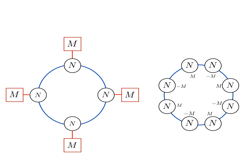
Figure V.2: The two circular-quiver gauge theories related by the $SL(2,\mathbb{Q})$ transformation (V.2.32). The theory on the right is obtained from the one on the left by doubling the number of gauge-group factors, removing the fundamental hypermultiplets and adding Chern-Simons terms with alternating sign.

As another example of $SL(2,\mathbb{Q})$ equivalence, we consider the transformation

$$\left(\begin{array}[]{cc}1&M^{-1}\\ 0&1\end{array}\right)\qquad{\rm with}\quad M\in\mathbb{N}\,.$$ (V.2.32)

This transformation leaves the NS5-branes invariant, while it converts a stack of $M$ D5-branes into a single $(1,M)$ five-brane. Recall that the worldvolume theory of a stack of $N$ D3-branes intersecting a stack of $M$ D5-branes is a $U(N)$ gauge theory with $M$ fundamental hypermultiplets and one adjoint hypermultiplet. Replacing the D5-branes by a $(1,M)$ five-brane leads to a $U(N)_{M}\times U(N)_{-M}$ gauge theory with one bifundamental hypermultiplet and level $M$ (respectively $-M$) Chern-Simons terms (see e.g. [1]). The transformation (V.2.32) can be used therefore to relate the following two theories:
(i) a $U(N)^{\hat{k}}$ gauge theory, with $M$ fundamental hypermultiplets for every gauge-group factor, and a bifundamental for each neighboring pair;
(ii) a $U(N)^{2\hat{k}}$ gauge theory with bifundamentals for each neighboring pair, and Chern-Simons terms of alternating level $\pm M$.
The corresponding circular quivers are illustrated in Figure V.2. As a test of their $SL(2,\mathbb{Q})$ equivalence we will conclude this section by comparing the free energies of these two gauge field theories in the limit $N\gg 1$.

Let us first recall the result (III.4.96) for the free energy on the supergravity side. Replacing the number of winding D3-branes by $N$, and the total number of D5-branes by $M\hat{k}$, leads to the expression

$$F_{\rm sugra}\,=\,\frac{\pi\sqrt{2}}{3}\hat{k}M^{1/2}\,N^{3/2}\ .$$ (V.2.33)

This should be compared to the result on the field-theory side. For the necklace quiver of theory (ii) the calculation has been performed in [35]. These authors used the localization techniques of [15] to reduce the calculation to a matrix-model integral, which they then evaluated for large-$N$ by the saddle-point method. Their result agrees precisely with (V.2.33), confirming the AdS/CFT correspondence. What we need to do is to also recover this result from the original gauge theory (i).

Since for theories with $\mathcal{N}\geq 4$ supersymmetries the free energy does not run [15], we may perform the calculation near the (ultraviolet) Gaussian fixed point. Using the standard localization techniques, one reduces the partition function of theory (i) to the following matrix-model integral:

$$Z_{(i)}={1\over(N!)^{\hat{k}}}\int\prod_{a=1}^{\hat{k}}\frac{d^{N}\sigma_{a}}{(2\pi)^{N}}\frac{\prod_{i<j}4\sinh^{2}\big{(}\frac{\sigma_{a}^{i}-\sigma_{a}^{j}}{2}\big{)}}{\prod_{i,j}2\cosh\big{(}\frac{\sigma_{a+1}^{i}-\sigma_{a}^{j}}{2}\big{)}}\frac{1}{\big{[}\prod_{j}2\cosh\big{(}\frac{\sigma_{a}^{j}}{2}\big{)}\big{]}^{M}}\ ,$$ (V.2.34)

where $i,j$ run from $1$ to $N$. This can be written as $Z_{(i)}=\int e^{-F(\sigma_{a})}$ with

$$F(\sigma_{a})\,=\,-2\sum_{a\,;\,i<j}\log\Big{[}2\sinh\big{(}\frac{\sigma_{a}^{i}-\sigma_{a}^{j}}{2}\big{)}\Big{]}+\sum_{a\,;\,i,j}\log\Big{[}2\cosh\big{(}\frac{\sigma_{a+1}^{i}-\sigma_{a}^{j}}{2}\big{)}\Big{]}$$

$$+\sum_{a\,;\,j}M\log\Big{[}2\cosh\big{(}\frac{\sigma_{a}^{j}}{2}\big{)}\Big{]}+\hat{k}\log(N!)+\hat{k}N\log(2\pi)\ .$$ (V.2.35)

Following reference [35], we let $\sigma_{a}^{j}=N^{\beta}x_{a}^{j}$, and fix $\beta$ so that at the saddle point the $x_{a}^{j}$ are of order one. Contrary to this reference, we do not introduce an imaginary part for the $x_{a}^{j}$. Indeed, the saddle point equations are invariant under complex conjugation, so we are entitled to look for real solutions.

In the limit $N\gg 1$, we may replace the variables $x_{a}^{i}$ by a continuous density $\rho_{a}(x)$ normalized so that $\int dx\rho_{a}(x)=1$. The expression V.2.35 can be written as

$$F(\rho_{a})=\sum_{a=1}^{\hat{k}} {1\over 2}\Big{[}{\pi^{2}}N^{2-\beta}\int dx_{a}\rho_{a}(x_{a})^{2}+{M}N^{1+\beta}\,\int dx_{a}|x_{a}|\rho_{a}(x_{a})\Big{]}$$ (V.2.36)

$$+O(N^{2-2\beta},N\log N)\ .$$

The details of the computation are subtle, at least to obtain the first term in V.2.36, and can be found in appendix A of [35].

The saddle-point equations are non-trivial when the two terms in this expression are of the same order, so that $\beta=\frac{1}{2}$. Furthermore, thanks to the symmetries of the problem, we may look for saddle points with $\rho_{a}(x)=\rho(x)$ for all $a$, and $\rho(x)=\rho(-x)$. With these assumptions the above free energy reduces to

$$F(\rho)=\frac{\hat{k}}{2}N^{\frac{3}{2}}\Big{[}\pi^{2}\int dx\,\rho(x)^{2}+M\int dx\,|x|\rho(x)-\gamma\int dx\,\rho(x)+\gamma\Big{]}\ ,$$ (V.2.37)

where the Lagrange multiplier $\gamma$ imposes the constraint $\int dx\rho(x)=1$. The ensuing saddle point equation,

$$2\pi^{2}\rho(x)+M|x|=\gamma\ ,$$ (V.2.38)

is solved by the eigenvalue density

$$\rho(x) =\frac{1}{2\pi^{2}}\big{(}\gamma-M|x|\big{)}\quad\textrm{for}\quad|x|<x_{0},$$

$$=0\quad\textrm{for}\quad|x|>x_{0}.$$ (V.2.39)

The constraint $\int dx\rho(x)=1$ fixes the Lagrange multiplier

$$\gamma=\frac{Mx_{0}}{2}+\frac{\pi^{2}}{x_{0}}\ ,$$ (V.2.40)

whereas the positivity of $\rho$ implies $x_{0}\leq\pi\sqrt{\frac{2}{M}}$. Combining all these formulae gives

$$F(x_{0})=\hat{k}N^{\frac{3}{2}}\Big{[}\frac{\pi^{2}}{4x_{0}}+\frac{Mx_{0}}{4}-\frac{M^{2}x_{0}^{3}}{48\pi^{2}}\Big{]}\ .$$ (V.2.41)

We now need to minimize this expression with respect to $x_{0}$ which takes values in $(0,\pi\sqrt{{2/M}}]$. The minimum is achieved at the rightmost endpoint, leading to the final result for the gauge theory (i):

$$F_{(i)}=\frac{\pi\sqrt{2}}{3}\hat{k}\sqrt{M}N^{\frac{3}{2}}\ ,$$ (V.2.42)

in perfect agreement with both the necklace-quiver and the supergravity calculations. Note that although the final results agree, the three calculations differ greatly in their specific details.

Perspectives

The AdS/CFT proposals that have been presented cover all the fixed points of 3d $\mathcal{N}=4$ linear quivers, circular quivers and $\frac{1}{2}$-BPS defect SCFTs preserving the supergroup $OSp(4|4)$. All the quarter-BPS brane configurations involving D3-branes, D5-branes and NS5-branes in type IIB string theory have been associated to a supergravity solution and quiver gauge theory. In this sense our classification seems complete. However new three dimensional $\mathcal{N}=4$ SCFTs associated to star-shaped quivers have been proposed in [36], raising the question of possible other supergravity solutions with the same symmetries. Although the construction of [36] is not completely clear to us, it is interesting to notice that the data needed for these star-quivers might match the parameters of supergravity solutions on a surface $\Sigma$ with a richer structure of boundary singularities, namely more boundary segments with D5 or NS5 singularities. The essential problem of these solutions is the presence of line singularities on $\Sigma$ or conical point singularities on $\Sigma$ with $2\pi$ deficit angle. The question of the existence of such solutions without singularity in the interior of $\Sigma$ is not settled. The question of the possible interpretation of the conical singularities is also open.

The question of dualities between the IIB solutions and IIA or M-theory solutions is also an interesting direction of investigations. For circular quiver geometries we have seen that the naive T-duality and lift to M-theory is related to the smeared IIB solution, where the surviving data is are just the total numbers of branes of each type. Recovering the 5-branes localization may follow from corrections to the metric due to worldsheet instantons as in [31], breaking the isometry of the T-duality. On the IIA side (resp. M-theory side) the information characterizing the quiver seems to be encoded in $B_{2}$ holonomies (resp. $C_{3}$ torsion fluxes) around the two-cycles (resp. three-cycles) of the geometry ([30]). This picture is not clear. The precise rules for the dualities should be clarified. The ABJM gauge theory might be a good place to start because we know its IIA, M-theory and now IIB supergravity duals.

We have also noticed that the domain wall supergravity solutions provide the string theory arena to explore the Karch-Randall scenario of localization of gravity in a non-compact internal space [16, 17]. Their model is based on 5d Einstein gravity with a negative cosmological constant in the presence of a 4-dimensional “thin brane”. The solution to the equations of motions for small enough thin-brane tension is an $AdS_{4}\ltimes\mathbb{R}$ fibration with a peak of the warp factor at the position of the thin brane. In this setup the first 4d graviton mode has a small mass and has its wavefunction localized near the thin-brane. Furthermore the rest of the graviton mass spectrum is separated from the lowest mass by a “large” mass gap. This provides an effective realization of 4d “almost massless”, “almost flat” gravity with a non-compact internal space, which is phenomenologically promising, except that the small 4d cosmological constant is negative. There was hope that this scenario can be realized in string theory with a brane configuration of D3-branes intersecting D5-branes. The near horizon geometries of such configurations are the one we have studied.
In [37] the fluctuations of the metric corresponding to the 4d gravitons were studied in detail for the case of the BPS Janus domain wall solution, which connects to $AdS_{5}\times S^{5}$ regions with different values of the dilaton. This corresponds to the absence of 5-branes in the geometry. It was shown that the Janus geometry does not reproduce the good features of the Karch-Randall model. The analysis for a situation with D5-branes and NS5-branes was essentially left for future work.
Our computations in the case of one stack of D5 and one stack of NS5-branes tend to show that the Karch-Randall scenario is again not reproduced. The main problem is that the favorable growth of the $AdS_{4}$ warp factor in the region near the 5-branes result in the formation of a quasi-flat central region of increasing size. Our analysis is presented in appendix E. Further work is still needed to evaluate the graviton mass spectrum and possibly explore richer geometries.

Chapter VI Appendices

A Mirror symmetry of inequalities

We will here show that the inequalities (II.3.36) are invariant under the mirror map, i.e. that

$$L+\rho^{T}>\hat{\rho}\ \ \Longleftrightarrow\ \ L+\hat{\rho}^{T}>\rho\ .$$ (A.1)

The proof of mirror symmetry for the linear quiver inequalities II.2.14 is then obtained simply by setting $L=0$.

Let us first recall that if $\tau=(a_{1},a_{2},...,a_{t})$ and $\sigma=(b_{1},b_{2},...,b_{s})$ are two partitions of the same number $N$, expressed as vectors with non-increasing positive components, then $L+\tau>\sigma$ is a shorthand notation for the set of inequalities

$$L+\sum_{i=1}^{n}a_{i}>\sum_{i=1}^{n}b_{i}\quad\quad\textrm{for\ all }\quad n=1,...,\textrm{max}(t,s).$$ (A.2)

These can be visualized more easily in the diagrammatic representation of figure VI.1, which defines a sequence $\{A_{1},A_{2},\cdots,A_{r}\}$ of areas with alternating signs. In terms of this sequence, the inequalities read

$$L+A_{1}>0\ ,\quad L+(A_{1}+A_{2})>0\ ,\quad\cdots\quad,\quad L+\sum_{s=1}^{r-1}A_{s}>0\ ,\quad L>0\ ,$$ (A.3)

where the last inequality follows from the fact that $A_{1}+A_{2}\cdots+A_{r}=0$. Reversing the order, one may put these inequalities in the following form:

$$L>0\ ,\quad L-A_{r}>0\ ,\quad L-A_{r}-A_{r-1}>0\ ,\cdots\quad,\quad L-\sum_{s=2}^{r}A_{s}>0\ .$$ (A.4)

This is exactly the set of inequalities corresponding to $L+\sigma^{T}>\tau^{T}$, as is evident if one transpose the figure VI.1.
Setting $\tau\equiv\rho^{T}$ and $\sigma\equiv\hat{\rho}$ proves the mirror equivalence (A.1), as claimed.

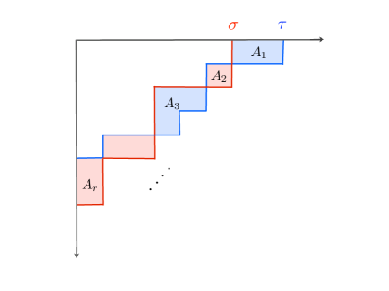
Figure VI.1: The difference of two Young tableaux defines an alternating sequence $\{A_{1},A_{2},\cdots,A_{r}\}$ where $|A_{i}|$ counts the number of boxes in the $i$th region enclosed by the two histograms of the Young tableaux. In this example $A_{1}=2,A_{2}=-1,A_{3}=3,\cdots$. The difference of the transposed tableaux, obtained by transposing the figure ($180^{\rm o}$ rotation around the descending diagonal), defines the inverse opposite sequence $\{-A_{r},\cdots,-A_{2},-A_{1}\}$.

B Proof of the inequalities in supergravity

In this appendix we prove the inequalities on the partitions $\rho$ and $\hat{\rho}$ required for the positivity of the ranks $N_{j}$ in the quiver dual description, which can be thought of as supersymmetry preserving conditions. We prove the inequalities for the supergravity solutions on the annulus, corresponding to circular quivers, keeping in mind that the inequalities for the solution on the strip, corresponding to linear quivers, are obtained in the limit $t\rightarrow\infty$ ($L\rightarrow 0$) as a (simpler) subcase. The computation can be easily adapted to the verification of inequalities for the domain wall supergravity solutions.

We have already shown in §III.3.3 that, with an appropriate choice of gauge, the linking numbers of the supergravity solution can be confined to the intervals $\ l^{(a)}\in(0,\hat{k}]$ and $\hat{l}^{(b)}\in(0,k]$. In particular, the linking numbers are positive, and we demand that they be quantized. Thus the Young tableaux $\rho$ and $\hat{\rho}$ are well defined, and the inequalities $L+\rho^{T}>\hat{\rho}$ make sense. We will now prove that these inequalities are automatically obeyed on the supergravity side.

Let us recall the explicit expressions of the five-brane linking numbers and of $L$:

$$l^{(a)} =\sum_{b=1}^{\hat{p}}\hat{N}_{b}\Big{[}\sum_{n=0}^{+\infty}f(\hat{\delta}_{b}-\delta_{a}-2nt)-\sum_{n=1}^{+\infty}f(-\hat{\delta}_{b}+\delta_{a}-2nt)\Big{]}\ ,$$

$$\hat{l}^{(b)} =\sum_{a=1}^{p}N_{a}\Big{[}\sum_{n=0}^{+\infty}f(\hat{\delta}_{b}-\delta_{a}-2nt)-\sum_{n=1}^{+\infty}f(-\hat{\delta}_{b}+\delta_{a}-2nt)\Big{]}\ ,$$ (B.5)

$$L =\sum_{a=1}^{p}\sum_{b=1}^{\hat{p}}\sum_{k=1}^{+\infty}k\ N_{a}\hat{N}_{b}\Big{[}f(\hat{\delta}_{b}-\delta_{a}-2kt)+f(\delta_{a}-\hat{\delta}_{b}-2kt)\Big{]}\ ,$$

where $f(x)=\frac{2}{\pi}\arctan(e^{x})$, and we use in this appendix a lighter notation for the five-brane charges, $N_{a}\equiv N^{(a)}_{5}$ and $\hat{N}_{b}\equiv\hat{N}^{(b)}_{5}$. In terms of these linking numbers and the five-brane charges the partitions $\hat{\rho}$ and $\rho^{T}$ read:

$$\hat{\rho} =(\underbrace{\hat{l}^{(1)},...,\hat{l}^{(1)}}_{\hat{N}_{1}},...,\underbrace{\hat{l}^{(b)},...,\hat{l}^{(b)}}_{\hat{N}_{b}},...,\underbrace{\hat{l}^{(\hat{p})},...,\hat{l}^{(\hat{p})}}_{\hat{N}_{\hat{p}}})\ ,$$ (B.6)

and

$$\rho^{T}=(\underbrace{\sum_{a=1}^{p}N_{a},...,\sum_{a=1}^{p}N_{a}}_{l^{(p)}},\underbrace{\sum_{a=1}^{p-1}N_{a},...,\sum_{a=1}^{p-1}N_{a}}_{l^{(p-1)}-l^{(p)}},...,\underbrace{\sum_{a=1}^{A}N_{a},...,\sum_{a=1}^{A}N_{a}}_{l^{(A)}-l^{(A+1)}},...,\underbrace{N_{1},...,N_{1}}_{l^{(1)}-l^{(2)}})\ .$$ (B.7)

We need now to establish the set of inequalities

$$\sum_{s=1}^{r}m_{s}\ +L\ > \ \sum_{s=1}^{r}\hat{l}_{s}\qquad\forall r=1,\ldots,\max(k,\hat{k})\,.$$ (B.8)

where $\hat{\rho}=(\hat{l}_{1},\hat{l}_{2},...,\hat{l}_{\hat{k}})$ and $\rho^{T}=(m_{1},m_{2},...,m_{k})$ are the above two partitions.

The last inequality, the one for $r=\max(k,\hat{k})$, implies that $L>0$. This is obeyed automatically, as seen from the explicit expression (B) and the fact that $f$ is strictly positive.

Let us show now that it is sufficient to prove the inequalities in (B.8) for the corners of the histogram $\hat{\rho}$, i.e. for the values

$$r=\sum_{b=1}^{J}\hat{N}_{b}\qquad{\rm where}\qquad J=1,2,...,\hat{p}\ .$$ (B.9)

To see why, assume that $r$ is in the range $\sum_{b=1}^{J-1}\hat{N}_{b}<r\leq\sum_{b=1}^{J}\hat{N}_{b}$, for some $J=1,2,...,\hat{p}$. Then if (B.8) is satisfied for all $r^{\prime}<r$ but not for $r$, it will not be satisfied for $r^{\prime\prime}=\sum_{b=1}^{J}\hat{N}_{b}$ either. This is because $\hat{l}_{s}$ is constant for $s$ in the range $\sum_{b=1}^{J-1}\hat{N}_{b}<s\leq\sum_{b=1}^{J}\hat{N}_{b}$, while the integer $m_{s}$, which belongs to a non-decreasing sequence of integers, does not increase as $s$ ranges over the values $\sum_{b=1}^{J-1}\hat{N}_{b}<s\leq\sum_{b=1}^{J}\hat{N}_{b}$. Conversely, if the constraint is satisfied for $r^{\prime\prime}$ then it will be satisfied also for $r$. We remark here that the limit of decoupled quivers, corresponding to disjoint brane configurations, is reached when the inequality is saturated for some value of $r$, with the saturation preserved for $r^{\prime}>r$. Following the logic of the previous argument, such an $r$ must be of the form $r=\sum_{b=1}^{J}\hat{N}_{b}$.

Let us now take a fixed $J$ with $1\leq J\leq\hat{p}$. By summing over the number of rows in $\rho^{T}$, we can always find an integer $I$ such that

$$l^{(I)}>r\geq l^{(I+1)}\ .$$ (B.10)

We may then write the sum over $m_{s}$ as

$$\sum_{s=1}^{r}m_{s} =\sum_{A=I+1}^{p}\sum_{a=1}^{A}N_{a}\left(l^{(A)}-l^{(A+1)}\right)+\left(r-l^{(I+1)}\right)\sum_{a=1}^{I}N_{a}$$ (B.11)

$$=\sum_{a=I+1}^{p}l^{(a)}N_{a}+\left(\sum_{b=1}^{J}\hat{N}_{b}\right)\left(\sum_{a=1}^{I}N_{a}\right)\ ,$$ (B.12)

where we have used (B.9) to replace $r$. The inequality (B.8) then becomes

$$\sum_{b=1}^{J}\hat{l}^{(b)}\hat{N}_{b}\ <\ L+\sum_{a=I+1}^{p}l^{(a)}N_{a}+\left(\sum_{a=1}^{I}N_{a}\right)\left(\sum_{b=1}^{J}\hat{N}_{b}\right)\ .$$ (B.13)

This is the form of the inequality that we will now prove using the supergravity calculation of the charges.

Let us give a name to the infinite sum that enters in the supergravity expressions for the linking numbers:

$$F(x,2t)\equiv\sum_{n=0}^{\infty}f(x-2nt)-\sum_{n=1}^{\infty}f(-x-2nt)\ .$$ (B.14)

In terms of the function $F$ the inequalities B.13 can be written as

$$\sum_{a=1}^{p}\sum_{b=1}^{J}N_{a}\hat{N}_{b}\,F(\hat{\delta}_{b}-\delta_{a},2t)\ <\ L+\sum_{a=I+1}^{p}\sum_{b=1}^{\hat{p}}N_{a}\hat{N}_{b}\,F(\hat{\delta}_{b}-\delta_{a},2t)+\sum_{a=1}^{I}\sum_{b=1}^{J}N_{a}\hat{N}_{b}\ .$$

Splitting the sums, simplifying and rearranging terms gives:

$$\sum_{a=1}^{I}\sum_{b=1}^{J}N_{a}\hat{N}_{b}\,F(\hat{\delta}_{b}-\delta_{a},2t)-\sum_{a=I+1}^{p}\sum_{b=J+1}^{\hat{p}}N_{a}\hat{N}_{b}\,F(\hat{\delta}_{b}-\delta_{a},2t)\ <\ L+\sum_{a=1}^{I}\sum_{b=1}^{J}N_{a}\hat{N}_{b}\ .$$

We show that this is automatically satisfied by putting the following successive bounds on the left hand side:

$$\ \hskip 42.67912pt\sum_{a=1}^{I}\sum_{b=1}^{J}N_{a}\hat{N}_{b}\,F(\hat{\delta}_{b}-\delta_{a},2t)-\sum_{a=I+1}^{p}\sum_{b=J+1}^{\hat{p}}N_{a}\hat{N}_{b}\,F(\hat{\delta}_{b}-\delta_{a},2t)$$

$$\ \hskip 8.5359pt<\ \sum_{a=1}^{I}\sum_{b=1}^{J}N_{a}\hat{N}_{b}\,\sum_{n=0}^{\infty}f(\hat{\delta}_{b}-\delta_{a}-2nt)+\sum_{a=I+1}^{p}\sum_{b=J+1}^{\hat{p}}N_{a}\hat{N}_{b}\,\sum_{n=1}^{\infty}f(-\hat{\delta}_{b}+\delta_{a}-2nt)$$

$$< \ \sum_{a=1}^{I}\sum_{b=1}^{J}N_{a}\hat{N}_{b}\ f(\hat{\delta}_{b}-\delta_{a})\ +\ \sum_{a=1}^{p}\sum_{b=1}^{\hat{p}}N_{a}\hat{N}_{b}\ \sum_{n=1}^{\infty}\Big{[}f(\hat{\delta}_{b}-\delta_{a}-2nt)+f(-\hat{\delta}_{b}+\delta_{a}-2nt)\Big{]}$$

$$\ \hskip 108.12054pt<\ L+\sum_{a=1}^{I}\sum_{b=1}^{J}N_{a}\hat{N}_{b}\ .$$ (B.15)

In the first inequality we have dropped terms that are explicitly negative. The second inequality is obtained by extension of the sums. Finally, in the third inequatlity we used, in addition to the bound $0<f(x)<1$, the expression (B) for the winding charge $L$. This completes the proof.

One can saturate the inequality $L>0$ by sending $t\rightarrow+\infty$ in which case $L\rightarrow 0$, obtaining a linear quiver geometry. In this limit ($t=+\infty$) we can saturate the inequality B.13 in two different manners:
(i) when $\delta_{a}\rightarrow+\infty$ for $a=I+1,I+2,...,p$ and $\hat{\delta}_{b}\rightarrow+\infty$ for $b=1,2,...,J$, or
(ii) when $\delta_{a}\rightarrow-\infty$ for $a=1,2,...,I$ and $\hat{\delta}_{b}\rightarrow-\infty$ for $j=J+1,J+2,...,\hat{p}$.

This limit corresponds to detaching a subset of fivebrane singularities and moving them off to infinity on the strip.

C From IIB to M theory for large $L$

We give here the detailed T-duality transformation of the type-IIB solution for large winding number $L$ to a solution of type-IIA supergravity, and the subsequent uplift to eleven dimensions. We will follow the metric, dilaton and two-form gauge fields, which all become part of the metric in eleven dimensions. The four-form potential of the IIB theory transforms to the three-form potential of M theory, which at leading order has a field strength proportional to the ${\rm AdS}_{4}$ volume form. The way in which the 3-form field may encode the information on the five-brane throats is a very subtle issue, as already noted in the main text. We will not discuss it further in this appendix.

The type-IIB backgrounds in the large-$L$ limit are given by the expressions (III.4.92) and (III.4.93). In order to use the standard Buscher rules, we make a gauge transformation that removes the $x$-dependence from the gauge potentials. The new two-form potentials read

$$B_{(2)} =-2\hat{k}\,\cos(\theta_{1})dx\wedge d\phi_{1}\ ,\qquad C_{(2)}=-2k\,\cos(\theta_{2})dx\wedge d\phi_{2}\ ,$$

where we recall that $x$ is periodic with period $2\pi$. We also transform the Einstein-frame to the string-frame metric, $G_{MN}=e^{\phi}g_{MN}$, in terms of which Buscher’s rules read [91]:

$$G^{\prime}_{\mu\nu} =G_{\mu\nu}-\frac{G_{x\mu}G_{x\nu}-B_{x\mu}B_{x\nu}}{G_{xx}}\ ,\qquad G^{\prime}_{0\nu}=\frac{B_{x\mu}}{G_{xx}}\ ,\qquad G^{\prime}_{xx}=\frac{1}{G_{xx}}\ ,$$

$$B^{\prime}_{\mu\nu} =B_{\mu\nu}-\frac{G_{x\mu}B_{x\nu}-B_{x\mu}G_{x\nu}}{G_{xx}}\ ,\qquad B^{\prime}_{0\nu}=\frac{G_{x\mu}}{G_{xx}}\ ,\qquad e^{4\phi^{\prime}}=\frac{e^{4\phi}}{G_{xx}}\ ,$$ (C.16)

where the prime indicates the type-IIA fields in string frame, and the lower-case Greek indices $\mu,\nu$ run over all dimensions other than $x$. In addition, the 2-form R-R potential transforms to a one-form potential,

$$C^{\prime}_{(1)\mu} =C_{(2)x\mu}\ .$$ (C.17)

Since the IIB metric had no $(x\mu)$ components $B^{\prime}$ is zero, while the original 2-form NS-NS gauge field becomes an off-diagonal component of the IIA metric. In string-frame this latter reads:

$$dS_{{\rm IIA}}^{\,2}= {{\pi^{2}\hat{k}}\over t}\sqrt{1-y}\left[ds^{2}_{AdS_{4}}+y\,ds^{2}_{S^{2}_{1}}+(1-y)ds^{2}_{S^{2}_{2}}\right]$$

$$+{4\pi^{2}\over t}\sqrt{1-y}\left[{y\over\hat{k}}(dx-{\hat{k}\over 2}{\rm cos}\theta_{1}d\phi_{1})^{2}+\hat{k}{dy^{2}\over y(1-y)}\right]\ ,$$ (C.18)

whereas the R-R gauge field and the transformed dilaton field are given by

$$C_{(1)}^{\prime}=-2k\,\cos\theta_{2}d\phi_{2}\ ,\qquad e^{4\phi^{\prime}}={4\pi^{2}\over t}{\hat{k}\over k^{2}}(1-y)^{3/2}\ .$$ (C.19)

Finally we uplift the solution to M theory, whose metric (denoted here by a bar) is given in terms of the type-IIA backgrounds by the following relations [117]

$$\bar{g}_{MN}=e^{-4\phi^{\prime}/3}(G^{\prime}_{MN}+{1\over 4}e^{4\phi^{\prime}}C^{\prime}_{M}C^{\prime}_{N})\ ,\quad\bar{g}_{Mv}=e^{8\phi^{\prime}/3}C^{\prime}_{M}\ ,\quad\bar{g}_{vv}=4e^{8\phi^{\prime}/3}\ ,$$ (C.20)

where $v=v+2\pi$ parametrizes the eleventh dimension. Redefining the coordinates $x\rightarrow\hat{k}x$ , $v\rightarrow kv$ and $y=\sin^{2}\alpha$ gives, after some straightforward algebra, the $AdS^{4}\times S^{7}/(\mathbb{Z}_{k}\times\mathbb{Z}_{\hat{k}})$ metric, equation (III.4.2).

D Barnes $G$-function

Let us briefly summarize the properties of the Barnes $G$-function. Barnes $G$-function $G_{2}(z)$ satisfies

$$G_{2}(z+1)=\Gamma(z)G_{2}(z),\quad G_{2}(1)=1\ .$$ (D.21)

From the definition it follows that

$$G_{2}(N)=(N-2)!(N-3)!\cdots 1!,\quad N=2,3,\cdots\ .$$ (D.22)

Its asymptotic expansion is given by

$$\ln G_{2}(N+1)=\frac{N^{2}}{2}\ln N-\frac{3}{4}N^{2}+\mathcal{O}(N)\ .$$ (D.23)

E Realization of the Karch-Randall model in domain wall supergravity solutions

In this appendix we explore the possibility of reproducing the Karch-Randall scenario of localization of a nearly massless graviton mode in our supergravity domain wall solutions (non-compact internal space). This short analysis follows the work of Bachas and Estes in [37]. First we present the essential features of the Karch-Randall model and then we study the first graviton mode in a simple domain wall solution. We explain qualitatively that the localization of gravity is not reproduced in this case, despites the presence of a nearly massless mode, because the region of localization decompactifies in the relevant limit.

E.1 The Karch-Randall scenario

In [16] Karch and Randall studied the graviton fluctuations in $AdS_{5}$ spacetime in the presence of a 4-dimensional ”thin brane” embedded in a $AdS_{4}$ slice. Their model is based on the effective 5-dimensional action

$$S_{KR} =-\frac{1}{2\kappa_{5}}\ \int d^{4}xdy\ \sqrt{g}\,\left(R+\frac{12}{L^{2}}\right)+\lambda\ \int d^{4}x\ \sqrt{[g]_{4}}\ ,$$ (E.24)

where $[g]_{4}$ is the induced metric at $y=0$. The coordinates $x^{\mu}$, $\mu=0,1,2,3$ parametrize the unit $AdS_{4}$ which is fibered over the direction $y$. $y=0$ is the position of the thin-brane. The parameters of the model are the 5D gravitational coupling $\kappa_{5}^{2}$, the bulk cosmological constant $\Lambda=-\frac{6}{L^{2}}$ and the tension $\lambda$ of the thin-brane.

Einstein equations are solved by the metric

$$ds^{2} =L^{2}\,\cosh^{2}\left(\frac{y_{0}-|y|}{L}\right)\ \bar{g}_{\mu\nu}dx^{\mu}dx^{\nu}+dy^{2}$$ (E.25)

with $\bar{g}_{\mu\nu}$ the metric of the unit radius $AdS_{4}$ and $y_{0}=L\ \textrm{arctanh}\left(\frac{\kappa_{5}^{2}\lambda L}{6}\right)$.

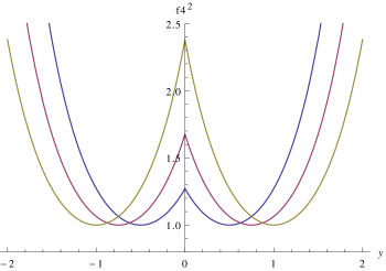
Figure VI.2: $AdS_{4}$ warp factor $f_{4}^{2}(y)\equiv L^{2}\cosh^{2}[(y_{0}-|y|)/L]$ of the Karch-Randall geometry for $L=1$ and $y_{0}=0.5,0.75,1$ from the smaller to the higher central pick respectively.

The geometry is characterized by the profile of its warp factor, which has two wells glued together at a distance $y_{0}$ from their centers, as shown in figure VI.2. The limit $y_{0}\rightarrow 0$ corresponds to having no thin-brane ($\lambda=0$) and the two wells fusionning to reconstruct the $AdS_{5}$ spacetime. The limit $y_{0}\rightarrow\infty$ corresponds to the two wells pushed apart far from each other and the spactimes splitting into two $AdS_{5}$. This limit corresponds to the thin-brane tension approaching (from below) a finite value $\lambda\rightarrow 6/\kappa_{5}^{2}L$. When $\lambda\geq 6/\kappa_{5}^{2}L$ the solutions to Einstein equations are 4-dimensional Minkovski or dS fibrations over the $y$ direction (see [16]).

The limit of phenomenological interest of the KR-model is $l^{2}>>L^{2}$ where

$$l^{2}=L^{2}\ \cosh^{2}\left(\frac{y_{o}}{L}\right)$$ (E.26)

is the $AdS_{4}$ warp factor at the location of the thin-brane $y=0$. This limit corresponds to $y_{0}$ larger than $L$ but not hierarchically larger. The graviton of 4-dimensional mass $m$ (in units of $1/L$) is defined by excitations of the unit $AdS_{4}$ metric $g_{\mu\nu}=\bar{g}_{\mu\nu}+h_{\mu\nu}$ and the ansatz

$$h_{\mu\nu}=h_{\mu\nu}^{[tt]}(x^{\sigma})\psi(y)$$ (E.27)

$$\bar{\Box}_{AdS_{4}}h_{\mu\nu}^{[tt]}=\left(m^{2}-2\right)\,h_{\mu\nu}^{[tt]}$$ (E.28)

$[tt]$ stands for “transverse traceless”. The case $m=0$ corresponds to a reduced number of polarization (massless or partially massless graviton) [118].

The mass spectrum contains excitations of mass $m=O(1)$ localized in the $AdS_{5}$ wells plus an additional zero mode localized on the thin-brane at $y=0$ of mass $m_{0}^{2}\simeq\frac{3L^{2}}{2l^{2}}$ ([119]). In the limit $L^{2}<<l^{2}$ this mode becomes nearly massless, with a mass gap with the other modes of order $\delta m=O(1)$.
At low energies the effective gravitational force is 4-dimensional Newton gravity localized near $y=0$. The corrections due to the other gaviton modes are suppressed by the presence of the mass gap, but also by the fact that their wavefunctions decrease exponentially fast apart from the $AdS_{5}$ wells, so that they are exponentially suppressed at $y=0$.

The interest of the KR model is that it realizes an effective theory containing 4-dimensional Newton’s gravity despites the presence of a non-compact internal space. This opens a new window for phenomenological models.

E.2 First graviton mass in a simple background

A simple background to explore the KR scenario is the near-horizon geometry of a set of D3-branes intersecting one stack of NS5-branes and one stack of D5-branes. More precisely we choose the supergavity solution on the strip with identical asymptotic $AdS_{5}\times S^{5}$ regions at $x=\pm\infty$, one stack of $\gamma$ D5-branes at $z=i\pi/2$ and one stack of $\gamma$ NS5-branes at $z=0$. We take the same number of 5-branes of each type, sitting at the same position in $x$ to stabilize the dilaton field in the region near the 5-branes, where the first graviton mode might be localized.
This is a 2-parameter solution, corresponding to the following choice of harmonic functions ($\alpha>0,\gamma>0$):

$$h_{1} =\,\left[-i\alpha\ {\rm sinh}(z)-\gamma\ {\rm ln}\left({\rm tanh}\left({i\pi\over 4}-{z\over 2}\right)\right)\right]+{\rm c.c.}\ ,$$

$$h_{2} =\,\left[\alpha\ {\rm cosh}(z)-\gamma\ {\rm ln}\left({\rm tanh}\left({z\over 2}\right)\right)\right]+{\rm c.c.}\ .$$ (E.29)

The corresponding geometry on the strip is depictedin figure VI.3.

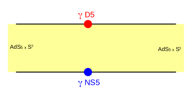
Figure VI.3: Strip geometry with asymptotic $AdS_{5}\times S^{5}$ regions ($x=\pm\infty$) of same radii, one stack of $\gamma$ D5-branes and one stack of $\gamma$ NS5-branes sitting in front of each other at $x=0$.

The asymptotic $AdS_{5}\times S^{5}$ radii are $L_{+}^{4}=L_{-}^{4}=16(\alpha^{2}+4\alpha\gamma)\equiv L^{4}$ (with $\alpha^{\prime}=4$) and the numbers of 5-branes are $N_{D5}=\mathcal{N}_{NS55}=\gamma$. Note that there is also a D3-flux $\pm N_{D3}=\gamma/2$ escaping from each 5-brane singularity. This means that in the flat brane picture we also have $\gamma/2$ D3-branes stretched between the NS5-branes and D5-branes. It would be interesting to study the case when these D3-branes are not there.

The limit of interest consists in having the asymptotic $AdS_{5}$ regions with fixed radius $L$, and to increase the number of 5-branes $\gamma$. This means $\alpha\gamma$ constant and $\gamma>>1$. The qualitative features of this limit are captured by the less restrictive limit $\gamma>>\alpha$, which is the limit we study.

One essential feature of the geometry E.2 is the $AdS_{4}$ warp factor $f_{4}^{2}$ illustrated in figure VI.4. In the limit $\gamma>>\alpha$ there is a central region of size $\sim\gamma^{1/2}\ln(\gamma/\alpha)$, which seems to become flat, connected on both sides to two fixtures, which are $AdS_{5}\times S^{5}$ wells with radius $L\simeq(\alpha\gamma)^{1/4}$, much smaller than the size of the central region.
The warp factor at the origin is given by $l^{2}\equiv f_{4}^{2}(x=0)\sim\gamma$. The ratio $L^{2}/l^{2}$ giving the scaling of the lowest mass of the KR model is then

$$m_{KR}^{2}\sim\frac{L^{2}}{l^{2}}\sim\left(\frac{\alpha}{\gamma}\right)^{\frac{1}{2}}\ .$$ (E.30)

As we will see now, the analysis of the first graviton mode does not seem to reproduce the same scaling.

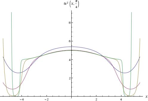
Figure VI.4: Warp factor $f_{4}^{2}$ of the $AdS_{4}$ metric as a function of the invariant distance $X[x]=\int_{0}^{x}2\rho(u,\pi/4)du$ evaluated on middle line $y=\pi/4$ of the strip, for $\gamma=1$ and $\alpha=10^{-1},10^{-2},10^{-4},10^{-6}$. When $\alpha$ decreases the two wells become narrower and the central region gets flatter.

Solving directly the spectral problem on the strip for the graviton in the presence of the fivebrane sources is a difficult issue. In order to understand the mass spectrum of gravitons, we chose to use variational tools, giving bounds on the masses. The discreteness of the spectrum, despites the non-compactness of the space, is a well-known property of $AdS$ spaces that acts like a box. What is of particular interest to us is the estimation of the lowest graviton mass and the mass gap between this first graviton and the rest of the spectrum. The phenomenologically interesting situation should combine the property of localization in space on the strip and the Karch-Randall mass hierarchy, which consists in a first mass much smaller than the mass gap between modes.

Here we only provide a numerical bound on the scaling of the first mass and comment qualitatively the situation, leaving a more serious analysis for a future work.

The graviton modes correspond to excitations of the 4-dimensional AdS part of the metric. The excitations on the two 2-spheres can be decomposed into Kaluza-Klein modes. Selecting the lowest mass mode means that we take the graviton to be constant on these 2-spheres. Following reference ([37]) we consider only perturbations $h_{\mu\nu}$ of the $AdS_{4}$ part of the metric:

$$ds^{2}=f_{4}^{2}\Big{(}\bar{g}_{\mu\nu}+h_{\mu\nu}\Big{)}dx^{\mu}dx^{\nu}+f_{1}^{2}ds^{2}_{S_{1}^{2}}+f_{2}^{2}ds^{2}_{S_{2}^{2}}+4\rho^{2}dzd\bar{z}$$ (E.31)

where $\bar{g}_{\mu\nu}$ is the $AdS_{4}$ metric with unit radius and $f_{4},f_{1},f_{2},\rho$ are the functions of $z,\bar{z}$ introduced in §III.2.1. We look for factorizable fluctuations with $AdS_{4}$ mass $m$ :

$$h_{\mu\nu}=h_{\mu\nu}^{[tt]}(x^{\sigma})\psi(z,\bar{z})$$ (E.32)

$$\bar{\Box}_{AdS_{4}}h_{\mu\nu}^{[tt]}=\left(m^{2}+\frac{2}{3}\Lambda\right)\,h_{\mu\nu}^{[tt]}$$ (E.33)

$[tt]$ stands for “transverse traceless” and $\Lambda$ is the cosmological constant of $AdS_{4}$ ($\Lambda=-3$ for unit radius). The mass in the 4d equation of motion for $h_{\mu\nu}^{[tt]}$ is defined so that the case $m=0$ corresponds to a reduced number of polarization (massless graviton) [118].

The linearized Einstein equations with this ansatz for the graviton fluctuations have been worked out in [37]. It turned out to be (universally) independent of the matter fields that the theory may contain and translates into a differential equation for $\psi$ on the strip. For the precise backgrounds given by the supergravity solutions that are studied in this presentation, the differential equation is given in terms of the two harmonic functions $h_{1},h_{2}$ by (see [37] for details)

$$2\frac{h_{1}h_{2}}{W}\ \partial\bar{\partial}\,\tilde{\psi}(z,\bar{z})=(2+m^{2})\tilde{\psi}(z,\bar{z})$$ (E.34)

where $W=\partial\bar{\partial}(h_{1}h_{2})$ and $\tilde{\psi}$ is related to the wavefunction on the strip $\psi$ by the relation $\tilde{\psi}=h_{1}h_{2}\,\psi$. The constant mode corresponds to $\tilde{\psi}=h_{1}h_{2}$ and is a local solution of this equation for $m=0$. Because of the unbounded asymptotic regions, this constant graviton mode is not normalizable.

One can show that the mass of the lightest mode $m_{0}$ depends only on the parameter $\frac{\alpha}{\gamma}$ because it is the only parameter appearing in the wave equation.

For any normalizable test function $\chi$, we have the following inequality with appropriate metric factor on the strip $\Sigma$ (with $z=x+iy$) :

$$2+m_{0}^{2}\quad\leq\quad\frac{\int\limits_{\Sigma}\chi^{\ast}O\chi|\frac{W}{h_{1}h_{2}}|dxdy}{\int\limits_{\Sigma}\chi^{\ast}\chi|\frac{W}{h_{1}h_{2}}|dxdy}\equiv 2+m_{00}^{2}$$ (E.35)

where $O\equiv 2\frac{h_{1}h_{2}}{W}\ \partial\bar{\partial}$ and the volume factor on the strip is given by $|\frac{W}{h_{1}h_{2}}|$ ([37]).

We can try to use this inequality with test functions that are close to the constant mode ($\tilde{\psi}=h_{1}h_{2}$) in the region between the two $AdS_{5}$ wells and close to zero outside, as the following test functions :

$$\chi(x,y)=\Big{(}\frac{1+\tanh(p(x+x_{0}))}{2}\Big{)}\Big{(}\frac{1+\tanh(p(-x+x_{0}))}{2}\Big{)}h_{1}h_{2}(x,y)$$

where $p$ can be adjusted for minimization and $x_{0}=\ln{\sqrt{\frac{\gamma}{\alpha}}}$ is the position of the well on the right of the strip (the left one being at position $-x_{0}$).

With the help of these test functions we obtained the graphic presented in figure VI.5.

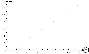
Figure VI.5: Numerical evaluation of an upper bound $m_{00}$ for the lightest mode for different values of $\gamma/\alpha$

The graphic is very close to a linear function of slope $1$, so we can infer the relation $m_{00}\propto\frac{\alpha}{\gamma}$, which means

$$m_{0}=O\left(\frac{\alpha}{\gamma}\right)$$ (E.36)

The conclusion from this simple analysis is that the first graviton mode has a mass which is even smaller than the naïve scaling of the Karch-Randall model E.30.

We recover the property that there is very light graviton localized in the central region. A complete analysis requires much more work. There are several types of other graviton modes : the modes that are localized in the $AdS_{5}$ wells will have (dimensionless) masses of order one as in the KR model, the Kaluza-Klein modes from the 2-spheres needs to be analysed, finally the presence of a nearly flat central region between the two $AdS_{5}$ wells indicates that there will be other graviton modes with their wavefunction localized in this region. To obtain an effective 4-dimensional Newton gravity, The masses of the modes localized in the central region should be large compared to the mass of the lowest mode.

The essential difference with the KR-model is the phenomenon of decompactification of the central region in the limit of large $\gamma$ : the first graviton mode does not seem to be localized near the position of the 5-branes, but rather it has a wavefunction quasi-constant on the whole region between the two $AdS_{5}$ wells. The size of this region is proportional to $\gamma^{1/2}\ln(\gamma/\alpha)$, so it decompactifies in the limit $\gamma>>1$, $\alpha\gamma$ fixed. Qualitatively we expect that in this limit the localization region gets larger and the coupling of the first mode to the other graviton modes tends to reproduce 5-dimensional gravity. This indicates that the KR scenario is not reproduced.

Index

Bibliography

- [1] O. Aharony, O. Bergman, D. L. Jafferis, and J. Maldacena, N=6 superconformal Chern-Simons-matter theories, M2-branes and their gravity duals, JHEP 0810 (2008) 091, [arXiv:0806.1218].
- [2] D. Martelli and J. Sparks, Moduli spaces of Chern-Simons quiver gauge theories and AdS(4)/CFT(3), Phys.Rev. D78 (2008) 126005, [arXiv:0808.0912].
- [3] D. Martelli and J. Sparks, AdS(40 / CFT(3) duals from M2-branes at hypersurface singularities and their deformations, JHEP 0912 (2009) 017, [arXiv:0909.2036].
- [4] D. L. Jafferis and A. Tomasiello, A Simple class of N=3 gauge/gravity duals, JHEP 0810 (2008) 101, [arXiv:0808.0864].
- [5] Y. Imamura and K. Kimura, On the moduli space of elliptic Maxwell-Chern-Simons theories, Prog.Theor.Phys. 120 (2008) 509–523, [arXiv:0806.3727].
- [6] F. Benini, C. Closset, and S. Cremonesi, Chiral flavors and M2-branes at toric CY4 singularities, JHEP 1002 (2010) 036, [arXiv:0911.4127].
- [7] A. Hanany, D. Vegh, and A. Zaffaroni, Brane Tilings and M2 Branes, JHEP 0903 (2009) 012, [arXiv:0809.1440].
- [8] B. Assel, C. Bachas, J. Estes, and J. Gomis, Holographic Duals of D=3 N=4 Superconformal Field Theories, JHEP 1108 (2011) 087, [arXiv:1106.4253].
- [9] B. Assel, C. Bachas, J. Estes, and J. Gomis, IIB Duals of D=3 N=4 Circular Quivers, JHEP 1212 (2012) 044, [arXiv:1210.2590].
- [10] B. Assel, J. Estes, and M. Yamazaki, Large N Free Energy of 3d N=4 SCFTs and AdS/CFT, arXiv:1206.2920.
- [11] D. Gaiotto and E. Witten, S-Duality of Boundary Conditions In N=4 Super Yang-Mills Theory, arXiv:0807.3720.
- [12] A. Hanany and E. Witten, Type IIB superstrings, BPS monopoles, and three-dimensional gauge dynamics, Nucl.Phys. B492 (1997) 152–190, [hep-th/9611230].
- [13] J. de Boer, K. Hori, H. Ooguri, and Y. Oz, Mirror symmetry in three-dimensional gauge theories, quivers and D-branes, Nucl.Phys. B493 (1997) 101–147, [hep-th/9611063].
- [14] D. Gaiotto and E. Witten, Supersymmetric Boundary Conditions in N=4 Super Yang-Mills Theory, arXiv:0804.2902.
- [15] A. Kapustin, B. Willett, and I. Yaakov, Exact Results for Wilson Loops in Superconformal Chern-Simons Theories with Matter, JHEP 1003 (2010) 089, [arXiv:0909.4559].
- [16] A. Karch and L. Randall, Locally localized gravity, JHEP 0105 (2001) 008, [hep-th/0011156].
- [17] A. Karch and L. Randall, Localized gravity in string theory, Phys.Rev.Lett. 87 (2001) 061601, [hep-th/0105108].
- [18] O. DeWolfe, D. Z. Freedman, and H. Ooguri, Holography and defect conformal field theories, Phys.Rev. D66 (2002) 025009, [hep-th/0111135].
- [19] J. Erdmenger, Z. Guralnik, and I. Kirsch, Four-dimensional superconformal theories with interacting boundaries or defects, Phys.Rev. D66 (2002) 025020, [hep-th/0203020].
- [20] D. Gaiotto and E. Witten, Janus Configurations, Chern-Simons Couplings, And The theta-Angle in N=4 Super Yang-Mills Theory, JHEP 1006 (2010) 097, [arXiv:0804.2907].
- [21] E. D’Hoker, J. Estes, and M. Gutperle, Exact half-BPS Type IIB interface solutions. I. Local solution and supersymmetric Janus, JHEP 0706 (2007) 021, [arXiv:0705.0022].
- [22] E. D’Hoker, J. Estes, and M. Gutperle, Exact half-BPS Type IIB interface solutions. II. Flux solutions and multi-Janus, JHEP 0706 (2007) 022, [arXiv:0705.0024].
- [23] T. Nishioka, Y. Tachikawa, and M. Yamazaki, 3d Partition Function as Overlap of Wavefunctions, JHEP 1108 (2011) 003, [arXiv:1105.4390].
- [24] J. M. Maldacena, The Large N limit of superconformal field theories and supergravity, Adv.Theor.Math.Phys. 2 (1998) 231–252, [hep-th/9711200].
- [25] E. Witten, Anti-de Sitter space and holography, Adv.Theor.Math.Phys. 2 (1998) 253–291, [hep-th/9802150].
- [26] O. Aharony, S. S. Gubser, J. M. Maldacena, H. Ooguri, and Y. Oz, Large N field theories, string theory and gravity, Phys.Rept. 323 (2000) 183–386, [hep-th/9905111].
- [27] S. de Haro, S. N. Solodukhin, and K. Skenderis, Holographic reconstruction of space-time and renormalization in the AdS / CFT correspondence, Commun.Math.Phys. 217 (2001) 595–622, [hep-th/0002230].
- [28] S. Gubser, I. R. Klebanov, and A. M. Polyakov, Gauge theory correlators from noncritical string theory, Phys.Lett. B428 (1998) 105–114, [hep-th/9802109].
- [29] B. M. Project, H. Bateman, and A. Erdélyi, Higher Transcendental Functions. No. vol. 2 in Higher Transcendental Functions. Dover Publications, Incorporated, 2007.
- [30] Y. Imamura and S. Yokoyama, N=4 Chern-Simons theories and wrapped M-branes in their gravity duals, Prog.Theor.Phys. 121 (2009) 915–940, [arXiv:0812.1331].
- [31] D. Tong, NS5-branes, T duality and world sheet instantons, JHEP 0207 (2002) 013, [hep-th/0204186].
- [32] S. Benvenuti and S. Pasquetti, 3D-partition functions on the sphere: exact evaluation and mirror symmetry, arXiv:1105.2551.
- [33] D. L. Jafferis, The Exact Superconformal R-Symmetry Extremizes Z, JHEP 1205 (2012) 159, [arXiv:1012.3210].
- [34] D. L. Jafferis, I. R. Klebanov, S. S. Pufu, and B. R. Safdi, Towards the F-Theorem: N=2 Field Theories on the Three-Sphere, JHEP 1106 (2011) 102, [arXiv:1103.1181].
- [35] C. P. Herzog, I. R. Klebanov, S. S. Pufu, and T. Tesileanu, Multi-Matrix Models and Tri-Sasaki Einstein Spaces, Phys.Rev. D83 (2011) 046001, [arXiv:1011.5487].
- [36] F. Benini, Y. Tachikawa, and D. Xie, Mirrors of 3d Sicilian theories, JHEP 1009 (2010) 063, [arXiv:1007.0992].
- [37] C. Bachas and J. Estes, Spin-2 spectrum of defect theories, JHEP 1106 (2011) 005, [arXiv:1103.2800].
- [38] E. D’Hoker and D. Z. Freedman, Supersymmetric gauge theories and the AdS / CFT correspondence, hep-th/0201253.
- [39] J. Polchinski, String Theory. Cambridge monographs on mathematical physics. Cambridge University Press, 1998.
- [40] E. Kiritsis, String Theory in a Nutshell. In a Nutshell. Princeton University Press, 2011.
- [41] J. Wess and J. Bagger, Supersymmetry and Supergravity. Princeton Series in Physics Series. University Press, 1992.
- [42] C. Johnson, D-Branes. Cambridge Monographs on Mathematical Physics. Cambridge University Press, 2006.
- [43] L. Andrianopoli and S. Ferrara, K-K excitations on AdS(5) x S**5 as N=4 ’primary’ superfields, Phys.Lett. B430 (1998) 248–253, [hep-th/9803171].
- [44] R. Emparan, C. V. Johnson, and R. C. Myers, Surface terms as counterterms in the AdS / CFT correspondence, Phys.Rev. D60 (1999) 104001, [hep-th/9903238].
- [45] K. Skenderis, Lecture notes on holographic renormalization, Class.Quant.Grav. 19 (2002) 5849–5876, [hep-th/0209067].
- [46] S. Kachru and E. Silverstein, 4-D conformal theories and strings on orbifolds, Phys.Rev.Lett. 80 (1998) 4855–4858, [hep-th/9802183].
- [47] E. Witten, Baryons and branes in anti-de Sitter space, JHEP 9807 (1998) 006, [hep-th/9805112].
- [48] J. Bagger and N. Lambert, Gauge symmetry and supersymmetry of multiple M2-branes, Phys.Rev. D77 (2008) 065008, [arXiv:0711.0955].
- [49] O. Aharony, O. Bergman, and D. L. Jafferis, Fractional M2-branes, JHEP 0811 (2008) 043, [arXiv:0807.4924].
- [50] V. E. Hubeny and M. Rangamani, A Holographic view on physics out of equilibrium, Adv.High Energy Phys. 2010 (2010) 297916, [arXiv:1006.3675].
- [51] S. A. Hartnoll, Lectures on holographic methods for condensed matter physics, Class.Quant.Grav. 26 (2009) 224002, [arXiv:0903.3246].
- [52] M. Marino, Lectures on localization and matrix models in supersymmetric Chern-Simons-matter theories, J.Phys. A44 (2011) 463001, [arXiv:1104.0783].
- [53] V. Balasubramanian and P. Kraus, A Stress tensor for Anti-de Sitter gravity, Commun.Math.Phys. 208 (1999) 413–428, [hep-th/9902121].
- [54] O. Aharony, A. Hanany, K. A. Intriligator, N. Seiberg, and M. Strassler, Aspects of N=2 supersymmetric gauge theories in three-dimensions, Nucl.Phys. B499 (1997) 67–99, [hep-th/9703110].
- [55] J. de Boer, K. Hori, H. Ooguri, Y. Oz, and Z. Yin, Mirror symmetry in three-dimensional theories, SL(2,Z) and D-brane moduli spaces, Nucl.Phys. B493 (1997) 148–176, [hep-th/9612131].
- [56] J. de Boer, K. Hori, and Y. Oz, Dynamics of N=2 supersymmetric gauge theories in three-dimensions, Nucl.Phys. B500 (1997) 163–191, [hep-th/9703100].
- [57] N. Seiberg and E. Witten, Gauge dynamics and compactification to three-dimensions, hep-th/9607163.
- [58] K. A. Intriligator and N. Seiberg, Mirror symmetry in three-dimensional gauge theories, Phys.Lett. B387 (1996) 513–519, [hep-th/9607207].
- [59] A. Kapustin, B. Willett, and I. Yaakov, Nonperturbative Tests of Three-Dimensional Dualities, JHEP 1010 (2010) 013, [arXiv:1003.5694].
- [60] N. Hama, K. Hosomichi, and S. Lee, Notes on SUSY Gauge Theories on Three-Sphere, JHEP 1103 (2011) 127, [arXiv:1012.3512].
- [61] N. Hama, K. Hosomichi, and S. Lee, SUSY Gauge Theories on Squashed Three-Spheres, JHEP 1105 (2011) 014, [arXiv:1102.4716].
- [62] I. Yaakov, Localization of gauge theories on the three-sphere, .
- [63] P. C. Argyres, M. R. Plesser, and N. Seiberg, The Moduli space of vacua of N=2 SUSY QCD and duality in N=1 SUSY QCD, Nucl.Phys. B471 (1996) 159–194, [hep-th/9603042].
- [64] A. Hanany and N. Mekareeya, Complete Intersection Moduli Spaces in N=4 Gauge Theories in Three Dimensions, JHEP 1201 (2012) 079, [arXiv:1110.6203].
- [65] V. Pestun, Localization of gauge theory on a four-sphere and supersymmetric Wilson loops, Commun.Math.Phys. 313 (2012) 71–129, [arXiv:0712.2824].
- [66] D. Gaiotto and P. Koroteev, On Three Dimensional Quiver Gauge Theories and Integrability, arXiv:1304.0779.
- [67] Y. Imamura and S. Yokoyama, Index for three dimensional superconformal field theories with general R-charge assignments, JHEP 1104 (2011) 007, [arXiv:1101.0557].
- [68] C. Krattenthaler, V. Spiridonov, and G. Vartanov, Superconformal indices of three-dimensional theories related by mirror symmetry, JHEP 1106 (2011) 008, [arXiv:1103.4075].
- [69] A. Kapustin and B. Willett, Generalized Superconformal Index for Three Dimensional Field Theories, arXiv:1106.2484.
- [70] T. Dimofte, D. Gaiotto, and S. Gukov, 3-Manifolds and 3d Indices, arXiv:1112.5179.
- [71] I. Yaakov, Redeeming Bad Theories, arXiv:1303.2769.
- [72] D. Bashkirov, Relations between supersymmetric structures in UV and IR for N=4 bad theories, arXiv:1304.3952.
- [73] M. R. Douglas and G. W. Moore, D-branes, quivers, and ALE instantons, hep-th/9603167.
- [74] P. Kronheimer, Instantons and the geometry of the nilpotent variety, J.Diff.Geom. 32 (1990) 473–490.
- [75] C. Bachas, J. Hoppe, and B. Pioline, Nahm equations, N=1* domain walls, and D strings in AdS(5) x S(5), JHEP 0107 (2001) 041, [hep-th/0007067].
- [76] J. Gomis and C. Romelsberger, Bubbling Defect CFT’s, JHEP 0608 (2006) 050, [hep-th/0604155].
- [77] H. Lin, O. Lunin, and J. M. Maldacena, Bubbling AdS space and 1/2 BPS geometries, JHEP 0410 (2004) 025, [hep-th/0409174].
- [78] J. T. Liu and W. Sabra, All 1/2 BPS solutions of IIB supergravity with SO(4) x SO(4) isometry, Phys.Lett. B658 (2007) 77–81, [hep-th/0611244].
- [79] O. Lunin, On gravitational description of Wilson lines, JHEP 0606 (2006) 026, [hep-th/0604133].
- [80] S. Yamaguchi, Bubbling geometries for half BPS Wilson lines, Int.J.Mod.Phys. A22 (2007) 1353–1374, [hep-th/0601089].
- [81] A. Karch and L. Randall, Open and closed string interpretation of SUSY CFT’s on branes with boundaries, JHEP 0106 (2001) 063, [hep-th/0105132].
- [82] K. Skenderis and M. Taylor, Branes in AdS and p p wave space-times, JHEP 0206 (2002) 025, [hep-th/0204054].
- [83] O. Aharony, L. Berdichevsky, M. Berkooz, and I. Shamir, Near-horizon solutions for D3-branes ending on 5-branes, Phys.Rev. D84 (2011) 126003, [arXiv:1106.1870].
- [84] D. N. Page, Classical Stability of Round and Squashed Seven Spheres in Eleven-Dimensional Supergravity, Phys.Rev. D28 (1983) 2976.
- [85] D. Marolf, Chern-Simons terms and the three notions of charge, hep-th/0006117.
- [86] K. Hosomichi, K.-M. Lee, S. Lee, S. Lee, and J. Park, N=4 Superconformal Chern-Simons Theories with Hyper and Twisted Hyper Multiplets, JHEP 0807 (2008) 091, [arXiv:0805.3662].
- [87] M. Benna, I. Klebanov, T. Klose, and M. Smedback, Superconformal Chern-Simons Theories and AdS(4)/CFT(3) Correspondence, JHEP 0809 (2008) 072, [arXiv:0806.1519].
- [88] E. Witten, Branes, Instantons, And Taub-NUT Spaces, JHEP 0906 (2009) 067, [arXiv:0902.0948].
- [89] O. Aharony, A. Hashimoto, S. Hirano, and P. Ouyang, D-brane Charges in Gravitational Duals of 2+1 Dimensional Gauge Theories and Duality Cascades, JHEP 1001 (2010) 072, [arXiv:0906.2390].
- [90] A. Dey, On Three-Dimensional Mirror Symmetry, JHEP 1204 (2012) 051, [arXiv:1109.0407].
- [91] T. Buscher, Path Integral Derivation of Quantum Duality in Nonlinear Sigma Models, Phys.Lett. B201 (1988) 466.
- [92] H. Ooguri and C. Vafa, Two-dimensional black hole and singularities of CY manifolds, Nucl.Phys. B463 (1996) 55–72, [hep-th/9511164].
- [93] R. Gregory, J. A. Harvey, and G. W. Moore, Unwinding strings and t duality of Kaluza-Klein and h monopoles, Adv.Theor.Math.Phys. 1 (1997) 283–297, [hep-th/9708086].
- [94] J. A. Harvey and S. Jensen, Worldsheet instanton corrections to the Kaluza-Klein monopole, JHEP 0510 (2005) 028, [hep-th/0507204].
- [95] N. Drukker, M. Marino, and P. Putrov, From weak to strong coupling in ABJM theory, Commun.Math.Phys. 306 (2011) 511–563, [arXiv:1007.3837].
- [96] M. Henneaux and C. Teitelboim, Dynamics of Chiral (selfdual) p forms, Phys.Lett. B206 (1988) 650.
- [97] S. B. Giddings, S. Kachru, and J. Polchinski, Hierarchies from fluxes in string compactifications, Phys.Rev. D66 (2002) 106006, [hep-th/0105097].
- [98] D. R. Gulotta, C. P. Herzog, and S. S. Pufu, From Necklace Quivers to the F-theorem, Operator Counting, and T(U(N)), arXiv:1105.2817.
- [99] A. Amariti and M. Siani, F-maximization along the RG flows: A Proposal, JHEP 1111 (2011) 056, [arXiv:1105.3979].
- [100] I. R. Klebanov, S. S. Pufu, and B. R. Safdi, F-Theorem without Supersymmetry, JHEP 1110 (2011) 038, [arXiv:1105.4598].
- [101] C. Closset, T. T. Dumitrescu, G. Festuccia, Z. Komargodski, and N. Seiberg, Contact Terms, Unitarity, and F-Maximization in Three-Dimensional Superconformal Theories, JHEP 1210 (2012) 053, [arXiv:1205.4142].
- [102] H. Casini, M. Huerta, and R. C. Myers, Towards a derivation of holographic entanglement entropy, JHEP 1105 (2011) 036, [arXiv:1102.0440].
- [103] H. Casini and M. Huerta, On the RG running of the entanglement entropy of a circle, Phys.Rev. D85 (2012) 125016, [arXiv:1202.5650].
- [104] A. Zamolodchikov, Irreversibility of the Flux of the Renormalization Group in a 2D Field Theory, JETP Lett. 43 (1986) 730–732.
- [105] Z. Komargodski and A. Schwimmer, On Renormalization Group Flows in Four Dimensions, JHEP 1112 (2011) 099, [arXiv:1107.3987].
- [106] J. H. Schwarz and P. C. West, Symmetries and Transformations of Chiral N=2 D=10 Supergravity, Phys.Lett. B126 (1983) 301.
- [107] C. Hull and P. Townsend, Unity of superstring dualities, Nucl.Phys. B438 (1995) 109–137, [hep-th/9410167].
- [108] K. Okuyama, Linear sigma models of H and KK monopoles, JHEP 0508 (2005) 089, [hep-th/0508097].
- [109] T. Kitao, K. Ohta, and N. Ohta, Three-dimensional gauge dynamics from brane configurations with (p,q) - five-brane, Nucl.Phys. B539 (1999) 79–106, [hep-th/9808111].
- [110] A. E. Lawrence, N. Nekrasov, and C. Vafa, On conformal field theories in four-dimensions, Nucl.Phys. B533 (1998) 199–209, [hep-th/9803015].
- [111] M. Bershadsky, Z. Kakushadze, and C. Vafa, String expansion as large N expansion of gauge theories, Nucl.Phys. B523 (1998) 59–72, [hep-th/9803076].
- [112] A. Armoni, M. Shifman, and G. Veneziano, Refining the proof of planar equivalence, Phys.Rev. D71 (2005) 045015, [hep-th/0412203].
- [113] P. Kovtun, M. Unsal, and L. G. Yaffe, Necessary and sufficient conditions for non-perturbative equivalences of large N(c) orbifold gauge theories, JHEP 0507 (2005) 008, [hep-th/0411177].
- [114] M. Hanada, C. Hoyos, and A. Karch, Generating new dualities through the orbifold equivalence: a demonstration in ABJM and four-dimensional quivers, JHEP 1201 (2012) 068, [arXiv:1110.3803].
- [115] M. Hanada, C. Hoyos, and H. Shimada, On a new type of orbifold equivalence and M-theoretic duality, Phys.Lett. B707 (2012) 394–397, [arXiv:1109.6127].
- [116] C. Bachas, I. Brunner, and D. Roggenkamp, A worldsheet extension of O(d,d:Z), arXiv:1205.4647.
- [117] E. Witten, String theory dynamics in various dimensions, Nucl.Phys. B443 (1995) 85–126, [hep-th/9503124].
- [118] S. Deser and A. Waldron, Stability of massive cosmological gravitons, Phys.Lett. B508 (2001) 347–353, [hep-th/0103255].
- [119] A. Miemiec, A Power law for the lowest eigenvalue in localized massive gravity, Fortsch.Phys. 49 (2001) 747–755, [hep-th/0011160].