Likelihood Robust Optimization for Data-driven Problems

Abstract

We consider optimal decision-making problems in an uncertain environment. In particular, we consider the case in which the distribution of the input is unknown, yet there is abundant historical data drawn from the distribution. In this paper, we propose a new type of distributionally robust optimization model called the likelihood robust optimization (LRO) model for this class of problems. In contrast to previous work on distributionally robust optimization that focuses on certain parameters (e.g., mean, variance, etc.) of the input distribution, we exploit the historical data and define the accessible distribution set to contain only those distributions that make the observed data achieve a certain level of likelihood. Then we formulate the targeting problem as one of optimizing the expected value of the objective function under the worst-case distribution in that set. Our model avoids the over-conservativeness of some prior robust approaches by ruling out unrealistic distributions while maintaining robustness of the solution for any statistically likely outcomes. We present statistical analyses of our model using Bayesian statistics and empirical likelihood theory. Specifically, we prove the asymptotic behavior of our distribution set and establish the relationship between our model and other distributionally robust models. To test the performance of our model, we apply it to the newsvendor problem and the portfolio selection problem. The test results show that the solutions of our model indeed have desirable performance.

1 Introduction

The study of decision making problems in uncertain environments has been a main focus in the operations research community for decades. In such problems, one has a certain objective function to optimize, however, the objective function depends not only on the decision variables, but also on some unknown parameters. Such situations are ubiquitous in practice. For example, in an inventory management problem, the inventory cost is influenced by both the inventory decisions and the random demands. Similarly, in a portfolio selection problem, the realized return is determined by both the choice of the portfolio and the random market fluctuations.

One solution method to such problems is stochastic optimization. In this approach, one assumes the knowledge of the distribution of the unknown parameters and chooses the decision that optimizes the expected value of the objective function. If the knowledge of the distribution is exact, then this approach is a precise characterization for a risk-neutral decision maker. Much research has been conducted on this topic; we refer the readers to Shapiro et al. [29] for a comprehensive review on the topic of stochastic optimization.

However, there are several drawbacks to the stochastic optimization approach. First, although stochastic optimization can frequently be formulated as a convex program, in order to solve it, one often has to resort to the Monte Carlo method, which can be computationally challenging. More importantly, due to the limitation of knowledge, the distribution of the uncertain parameters is rarely known in practice to a precise level. Even if enough data have been gathered in the past to perform statistical analyses for the distribution, the analyses are often based on assumptions (e.g., independence of the observations, or stationarity of the sequence) that are only approximations of the reality. In addition, many decision makers in practice are not risk-neutral. They tend to be risk-averse. A solution approach that can guard them from adverse scenarios is of great practical interest.

One such approach was proposed by Scarf [27] in a newsvendor context and has been studied extensively in the past decade. It is called the distributionally robust optimization (DRO) approach. In the DRO approach, one considers a set of distributions for the uncertain parameters and optimizes the worst-case expected value of the objective function among the distributions in that set. Studies have been done by choosing different distribution sets. Among them, most choose the distribution set to contain those distributions with a fixed mean and variance. For example, Scarf [27] shows that a closed-form solution can be obtained in the newsvendor problem context when such a distribution set is chosen. Other earlier works include Gallego and Moon [15], Dupaĉová [14] and Ẑáĉková [34]. The same form of the distribution set is also used in Calafiore and El Ghaoui [10], Yue et al. [33], Zhu et al. [35] and Popescu [26] in which a linear-chance-constrained problem, a minimax regret objective and a portfolio optimization problem are considered, respectively. Other distribution sets beyond the mean and variance have also been proposed in the literature. For example, Delage and Ye [13] propose a more general framework with a distribution set formed by moment constraints. A review of the recent developments can be found in Delage [12] and Shapiro and Klegwegt [30].

Although the mean-variance DRO approach is intuitive and is tractable under certain conditions, it is unsatisfactory from at least two aspects. First, when constructing the distribution set in such an approach, one only uses the moment information in the sample data, while all the other information is ignored. This procedure may discard important information in the data set. For example, a set of data drawn from an exponential distribution with $\lambda=1/50$ will have similar mean and variance as a set of data drawn from a normal distribution with $\mu=\sigma=50$. In the mean-variance DRO, they will result in the same distribution set and the same decision will be chosen. However, these two distributions have very different properties and the optimal decisions may be quite different. Second, in the DRO approach, the worst-case distribution for a decision is often unrealistic. For example, Scarf [27] shows that the worst-case distribution in the newsvendor context is a two-point distribution. This raises the concern that the decision chosen by this approach is guarding some overly conservative scenarios, while performing poorly in more likely scenarios. Unfortunately, these drawbacks seem to be inherent in the model choice and cannot be satisfactorily remedied.

In this paper, we propose another choice of the distribution set in the DRO framework that solves the above two drawbacks of the mean-variance approach. Instead of using the mean and variance to construct the distribution set, we choose to use the likelihood function. More precisely, given a set of historical data, we define the distribution set to be the set of distributions that make the observed data achieve a certain level of likelihood. We call this approach the likelihood robust optimization (LRO) approach. The goal of this paper is to study the properties of LRO and its performance.

First, we show that the LRO model is highly tractable. By applying the duality theory, we formulate the robust counterpart of this problem into a single convex optimization problem. In addition, we show that our model is very flexible. We can add any convex constraints (such as the moment constraints) to the distribution set while still maintaining its tractability. Two concrete examples (a newsvendor problem and a portfolio selection problem) are discussed in the paper to illustrate the applicability of our framework.

Then we study the statistical theories behind the LRO approach by illustrating the linkage between our approach and the Bayesian statistics and empirical likelihood theory. We show that the distribution set in our approach can be viewed as a confidence region for the distributions given the set of observed data. Then we discuss how to choose the parameter in the distribution set to attain a specified confidence level. Furthermore, we show a connection between the LRO approach and the mean-variance DRO approach. Our analysis shows that the LRO approach is fully data-driven, and it takes advantage of the full strength of the available data while maintaining a certain level of robustness.

Finally, we test the performance of the LRO model in two problems, a newsvendor problem and a portfolio selection problem. In the newsvendor problem, we find that our approach produces similar results compared to the mean-variance DRO approach when the underlying distribution is symmetric, while the solution of our approach is much better when the underlying distribution is asymmetric. In the portfolio selection problem, we show by using real historical data that our approach achieves decent returns. Furthermore, the LRO approach will naturally diversify the portfolio. As a result, the returns of the portfolio have a relatively small fluctuation.

Following the initial version of this paper, Ben-Tal et al. [1] studied a distributionally robust optimization model where the distribution set is defined by divergence measures. Their model contains the LRO as a special case. They also discuss solvability and the statistical properties of their models. In this paper, we focus on the distribution set defined by the likelihood function and further explore the connections to the empirical likelihood theory. In addition, we also address the scenario when the sample space is continuous, which adds insights to this class of approaches.

Besides the paper by Ben-Tal et al. [1], a recent paper by Bertsimas et al. [6] also studies DRO with various choices of the distribution set. In particular, they focus on using data and hypothesis-testing tools to construct those sets. Although their paper is similar to ours, they do not use the likelihood function to construct the robust distribution set nor do they further study the properties of the DRO with such distribution sets.

Two other papers related to this one are Iyengar [17] and Nilim and El Ghaoui [22]. In these two papers, the authors study the robust Markov Decision Process (MDP) problem in which the transition probabilities can be chosen from a certain set. They mention the likelihood set as one choice. However, they do not further explore the properties of this set or attempt to extend it to general problems.

The remainder of this paper is organized as follows: In Section 2, we introduce our likelihood robust optimization framework and discuss its tractability and statistical properties. In Section 3, we extend our discussions to problems with continuous state space. In Section 4, we present numerical tests of our model. Section 5 concludes this paper.

2 Likelihood Robust Optimization Model

In this section, we formulate the likelihood robust optimization (LRO) model, discuss its tractability and statistical properties. We only consider the case where the uncertainty parameters have a finite discrete support in this section. We will extend our discussions to the case with continuous support in Section 3.

Suppose we want to maximize an objective function $h(\mbox{\boldmath$x$},\mbox{\boldmath$\xi$})$ where $x$ is the decision variable with feasible set $D$, and $\xi$ is a random variable taking values in $\Xi=\{\mbox{\boldmath$\xi$}_{1},\mbox{\boldmath$\xi$}_{2},...,\mbox{\boldmath$\xi$}_{n}\}$. The set $\Xi$ is known in advance. Assume we have observed $N$ independent samples of $\xi$, with $N_{i}$ occurrences of $\mbox{\boldmath$\xi$}_{i}$. We define:

$${\mathbb{D}}(\gamma)=\left\{\mbox{\boldmath$p$}=(p_{1},p_{2},...,p_{n})\left|\sum_{i=1}^{n}N_{i}\log{p}_{i}\geq\gamma,\sum_{i=1}^{n}p_{i}=1,p_{i}\geq 0,\forall i=1,...,n\right.\right\}.$$ (1)

We call ${\mathbb{D}}(\gamma)$ the likelihood robust distribution set with parameter $\gamma$. Note that ${\mathbb{D}}(\gamma)$ contains all the distributions with support in $\Xi$ such that the observed data achieves an empirical likelihood of at least $\exp(\gamma)$. At this point, we treat $\gamma$ as a given constant. Later we will discuss how to choose $\gamma$ such that (1) has a desirable statistical meaning. We formulate the LRO problem as follows:

$$\mbox{maximize}_{\mbox{\boldmath$x$}\in D} \left\{\min_{\mbox{\boldmath$p$}\in{\mathbb{D}(\gamma)}}\mbox{ }\sum_{i=1}^{n}p_{i}h(\mbox{\boldmath$x$},\mbox{\boldmath$\xi$}_{i})\right\}.$$ (2)

In (2), we choose the decision variable $x$, such that the expectation of the objective function under the worst-case distribution is maximized, where the worst-case distribution is chosen among the distributions such that the observed data achieve a certain level of likelihood. Prior to this work, researchers have chosen other types of distribution sets for the inner problem in (2), e.g., distributions with moment constraints. Works of that type have been reviewed in Section 1.

Here we comment on our assumption of the known support of the random variable $\xi$. In the LRO, the choice of $\Xi$ is important; a different choice of $\Xi$ will result in a different distribution set and a different solution to the decision problem. In practice, sometimes $\Xi$ has a clear definition. For example, if $\xi$ is the transition indicator of a Markov chain (thus those $p$s are transition probabilities), then the set of $\Xi$ is simply all the attainable states in the Markov chain. However, in cases where the choice of $\Xi$ is less clear, e.g., when $\xi$ represents the return of certain assets, the decision maker should choose $\Xi$ to reflect his view of plausible outcomes. Also, as we will show later, one can sometimes add other constraints such as moment constraints into the distribution set. Once such constraints are added, the choice of support often becomes less critical, since the support may be constrained by existing constraints.

2.1 Tractability of the LRO Model

In this subsection, we show that the LRO model is easily solvable. To solve (2), we write down the Lagrangian of the inner optimization problem:

$$L(\mbox{\boldmath$p$},\lambda,\mu)=\sum_{i=1}^{n}p_{i}h(\mbox{\boldmath$x$},\mbox{\boldmath$\xi$}_{i})+\lambda\left(\gamma-\sum_{i=1}^{n}N_{i}\log{p_{i}}\right)+\mu\left(1-\sum_{i=1}^{n}p_{i}\right).$$

Therefore, the dual formulation of the inner problem is

$$\mbox{maximize}_{\lambda,\mu} \mu+\lambda\left(\gamma+N-\sum_{i=1}^{n}N_{i}\log{N_{i}}\right)-N\lambda\log{\lambda}+\lambda\sum_{i=1}^{n}N_{i}\log{(h(\mbox{\boldmath$x$},\mbox{\boldmath$\xi$}_{i})-\mu)}$$

s.t. $$\lambda\geq 0,\quad h(\mbox{\boldmath$x$},\mbox{\boldmath$\xi$}_{i})-\mu\geq 0,\quad\forall i.$$ (3)

Since the inner problem of (2) is always convex and has an interior solution (given it is feasible), the optimization problem (2.1) always has the same optimal value as (2) (see, e.g., Boyd and Vandenberghe [9]). Then we combine (2.1) and the outer maximization problem. We have that (2) is equivalent to the following:

$$\mbox{maximize}_{\mbox{\boldmath$x$},\lambda,\mu} \mu+\lambda(\gamma+N-\sum_{i=1}^{n}N_{i}\log{N_{i}})-N\lambda\log{\lambda}+\lambda\sum_{i=1}^{n}N_{i}\log{(h(\mbox{\boldmath$x$},\mbox{\boldmath$\xi$}_{i})-\mu)}$$

s.t. $$\lambda\geq 0,\quad h(\mbox{\boldmath$x$},\mbox{\boldmath$\xi$}_{i})-\mu\geq 0,\mbox{ }\forall i,\quad\mbox{\boldmath$x$}\in D.$$ (4)

The following proposition follows immediately from examining the convexity of the problem and studying its KKT conditions.

Proposition 1.

If $h(\mbox{\boldmath$x$},\mbox{\boldmath$\xi$})$ is concave in $x$, then the likelihood robust optimization problem described in (2) can be solved by solving (2.1), which is a convex optimization problem. Furthermore, if $(\mbox{\boldmath$x$}^{*},\lambda^{*},\mu^{*},\mbox{\boldmath$y$}^{*})$ is an optimal solution for (2.1), then

$$p_{i}=\frac{\lambda^{*}N_{i}}{h(\mbox{\boldmath$x$}^{*},\mbox{\boldmath$\xi$}_{i})-\mu^{*}}$$

is the corresponding worst-case distribution.

One advantage of the LRO approach is that one can integrate the mean, variance and/or certain other information that is convex in $p$ into the distribution set. For example, if one wants to impose additional linear constraints on $p$, say $A\mbox{\boldmath$p$}\geq\mbox{\boldmath$b$}$ (note that this includes moment constraints as a special case), then the likelihood robust optimization model can be generalized as follows:

$$\mbox{maximize}_{\mbox{\boldmath$x$}\in D} \mbox{min}_{\mbox{\boldmath$p$}\in{\mathbb{D}(\gamma)},A\mbox{\boldmath$p$}\geq\mbox{\boldmath$b$}} \sum_{i=1}^{n}p_{i}h(x,\mbox{\boldmath$\xi$}_{i}).$$ (5)

By applying the duality theory again, we can transform (5) into the following problem ($\mu$ is the dual variable associated with the constraint $A\mbox{\boldmath$p$}\geq\mbox{\boldmath$b$}$, and we assume that $\sum_{i=1}^{n}p_{i}=1$ has been incorporated into $A\mbox{\boldmath$p$}\geq\mbox{\boldmath$b$}$):

$$\mbox{maximize}_{\mbox{\boldmath$x$},\lambda,\mbox{\boldmath$\mu$}} \mbox{\boldmath$b$}^{T}\mbox{\boldmath$\mu$}+(\gamma+N-\sum_{i=1}^{n}N_{i}\log{N_{i}})\cdot\lambda-N\lambda\log{\lambda}+\lambda\sum_{i=1}^{n}N_{i}\log{(h(\mbox{\boldmath$x$},\mbox{\boldmath$\xi$}_{i})-\mbox{\boldmath$a$}_{i}^{T}\mbox{\boldmath$\mu$})}$$

s.t. $$h(\mbox{\boldmath$x$},\mbox{\boldmath$\xi$}_{i})-\mbox{\boldmath$a$}_{i}^{T}\mbox{\boldmath$\mu$}\geq 0,\mbox{ }\forall i$$

$$\mbox{\boldmath$x$}\in D,\mbox{\boldmath$\mu$}\geq 0,\lambda\geq 0,$$

which is again a convex program and readily solvable.

2.2 Statistical Properties of the LRO Model

In this subsection, we study the statistical theory behind the LRO model. Specifically, we focus on the likelihood robust distribution set defined in (1). We will address the following questions:

1. What are the statistical meanings of (1)?

2. How does one select a meaningful $\gamma$?

3. How does the LRO model relate to other types of distributionally robust optimization models?

We answer the first question in Section 2.2.1 by using the Bayesian statistics and empirical likelihood theory to interpret the likelihood constraints. Those interpretations clarify the statistical motivations of the LRO model. Then we answer the second question in Section 2.2.2 in which we perform an asymptotic analysis of the likelihood region and point out an asymptotic optimal choice of $\gamma$. We study the last question in Section 2.2.3 where we present a relationship between our model and the traditional mean robust optimization model.

2.2.1 Bayesian Statistics Interpretation

Consider a random variable taking values in a finite set $S$. Without loss of generality, we assume $S=\{1,...,n\}$. Assume the underlying probability distribution of the random variable is $\mbox{\boldmath$p$}=\{p_{1},...,p_{n}\}$. We observe historical data $\Psi=\{N_{1},...,N_{n}\}$ in which $N_{k}$ represents the number of times the random variable takes value $k$. Then the maximum likelihood estimate (MLE) of $p$ is given by $(N_{1}/N,N_{2}/N,...,N_{n}/N)$ where $N=\sum_{i=1}^{n}N_{i}$ is the total number of observations.

Now we examine the set of distributions $p$ such that the likelihood of $\Psi$ under $p$ exceeds a certain threshold. We use the concepts from Bayesian statistics (see e.g., Gelman et al. [16]). Instead of thinking that the data are randomly drawn from the underlying distribution, we treat them as given, and we define a random vector $\mbox{\boldmath$p$}=(p_{1},...,p_{n})$ taking values on the $(n-1)$-dimensional simplex $\Delta=\{\mbox{\boldmath$p$}|p_{1}+\cdots+p_{n}=1,p_{i}\geq 0\}$ with probability density function proportional to the likelihood function:

$$\prod_{i=1}^{n}{p_{i}}^{N_{i}}.$$

This distribution of $p$ is known as the Dirichlet distribution. A Dirichlet distribution with parameter $\Psi$ (denoted by $Dir(\Psi)$) has the density function as follows:

$$f(\mbox{\boldmath$p$};\Psi)=\frac{1}{B(\Psi)}\prod_{i=1}^{n}{p_{i}}^{N_{i}-1}$$

with

$$B(\Psi)=\int_{\mbox{\boldmath$p$}\in\Delta}\prod_{i=1}^{n}{p_{i}}^{N_{i}-1}dp_{1}\cdots dp_{n}=\frac{\prod_{i=1}^{n}\Gamma(N_{i})}{\Gamma(\sum_{i=1}^{n}N_{i})},$$

where $\Gamma(\cdot)$ is the Gamma function. The Dirichlet distribution is used to estimate the unknown parameters of a discrete probability distribution given a collection of samples. Intuitively, if the prior distribution is represented as $Dir(\mbox{\boldmath$\alpha$})$, then $Dir(\mbox{\boldmath$\alpha$}+\mbox{\boldmath$\beta$})$ is the posterior distribution following a sequence of observations with histogram $\beta$. For a detailed discussion on the Dirichlet distribution, we refer the readers to [16].

In the LRO model, we assume a uniform prior $Dir(\mbox{\boldmath$e$})$ on each point in the support of the data, where $e$ is the unit vector. After observing the historical data $\Psi$, the posterior distribution follows $Dir(\Psi+\mbox{\boldmath$e$})$. Note that this process can be adaptive as we observe new data.

Now we turn to examine the likelihood robust distribution set

$${\mathbb{D}}(\gamma)=\left\{\mbox{\boldmath$p$}\left|\sum_{i=1}^{n}N_{i}\log{p_{i}}\geq\gamma,\sum_{i=1}^{n}p_{i}=1,p_{i}\geq 0,\forall i=1,...,n\right.\right\}.$$ (6)

This set represents a region in the probability distribution space. In the Bayesian statistics framework, we can compute the probability that $p$ satisfies this constraint:

$${\mathbb{P}}^{*}\left(\mbox{\boldmath$p$}\in{\mathbb{D}}(\gamma)\right)=\frac{1}{B(\Psi+\mbox{\boldmath$e$})}\int_{\mbox{\boldmath$p$}\in\Delta}\prod_{i=1}^{n}{p_{i}}^{N_{i}}\cdot{\mathbb{I}}\left(\sum_{i=1}^{n}N_{i}\log{p_{i}}\geq\gamma\right)dp_{1}\cdots dp_{n},$$

where ${\mathbb{P}}^{*}$ is the probability measure of $p$ given the observed data $\Psi$ (thus ${\mathbb{P}}^{*}$ is the probability measure under $Dir(\Psi+\mbox{\boldmath$e$})$), and ${\mathbb{I}}(\cdot)$ is the indicator function. When choosing the likelihood robust distribution set, we want to choose $\gamma^{*}$ such that

$${\mathbb{P}}^{*}\left(\mbox{\boldmath$p$}\in{\mathbb{D}}(\gamma^{*})\right)\geq 1-\alpha$$ (7)

for some predetermined $\alpha$. That is, we want to choose $\gamma^{*}$ such that (6) is the $1-\alpha$ confidence region of the probability parameters. The LRO model can then be interpreted as choosing the decision variable to maximize the worst-case objective where the worst-case distribution is chosen from the confidence region defined by the observed data.

However, in general, trying to find the exact $\gamma^{*}$ that satisfies (7) is computationally challenging. In the next subsection, we study the asymptotic properties of $\gamma^{*}$, which help us to approximate it.

2.2.2 Asymptotic Analysis of the Likelihood Robust Distribution Set

Now we investigate the asymptotic behavior of the likelihood robust distribution set and give an explicit way to choose an appropriate $\gamma$ in the LRO model. In this section, we assume that the true underlying distribution of the data is $\bar{\mbox{\boldmath$p$}}=\{\bar{p}_{1},...,\bar{p}_{n}\}$ with $\bar{p}_{i}>0$. We observe $N$ data drawn randomly from the underlying distribution with $N_{i}$ observations on outcome $i$ ($\sum_{i=1}^{n}N_{i}=N$). We define $\gamma_{N}$ to be the solution such that

$$\mathbb{P}_{\mbox{\boldmath$N$}}\left(\mbox{\boldmath$p$}\in{\mathbb{D}}(\gamma_{N})\right)=1-\alpha.$$

Here $\alpha$ is a fixed constant and $\mathbb{P}_{\mbox{\boldmath$N$}}$ is the Dirichlet probability measure on $p$ with parameters $N_{1},...,N_{n}$. Clearly $\gamma_{N}$ depends on $N_{i}$ and thus is a random variable. We have the following theorem about the asymptotic properties of $\gamma_{N}$, whose proof is referred to Pardo [24]. (We use $\rightarrow_{p}$ to mean “converge in probability.”)

Theorem 1.

$$\gamma_{N}-\sum_{i=1}^{n}N_{i}\log{\frac{N_{i}}{N}}\rightarrow_{p}-\frac{1}{2}\chi^{2}_{n-1,1-\alpha}$$

where $\chi^{2}_{d,1-\alpha}$ is the $1-\alpha$ quantile of a $\chi^{2}$ distribution with $d$ degrees of freedom.

Theorem 1 provides a heuristic guideline on how to choose the threshold $\gamma$ in the LRO model. In particular, one should choose approximately

$$\gamma^{*}=\sum_{i=1}^{n}{N_{i}}\log{\frac{N_{i}}{N}}-\frac{1}{2}\chi^{2}_{n-1,1-\alpha}$$

in order for the likelihood robust distribution set to have a confidence level of $1-\alpha$. Note that the difference between $\gamma^{*}$ and $\sum_{i}N_{i}\log{(N_{i}/N)}$ converges as $N$ grows. This means that when the data set is large, the allowable distributions must be very close to the empirical data. This is unlike some other distributionally robust optimization approaches which construct the distribution sets based on the mean and/or the variance. Even with large data size, the distribution set in those approaches may still contain distributions that are far from the empirical distribution, such as a two-point distribution at the ends of an interval. Therefore our approach does a better job in utilizing the historical data to construct the robust region.

We also have a theorem about the convergence speed of $\gamma_{N}$. We use $\Rightarrow_{d}$ to denote “converge in distribution.”

Theorem 2.

$$\sqrt{N}\left(\frac{\gamma_{N}}{N}-\sum_{i=1}^{n}\bar{p}_{i}\log{\bar{p}_{i}}\right)\Rightarrow_{d}X_{0},$$

where $X_{0}=\sum_{i=1}^{n}(1+\log{\bar{p}_{i}})X_{i}$ with $(X_{1},...,X_{n})\sim N(0,\Sigma)$ where

$$\Sigma=\left(\begin{array}[]{cccc}\bar{p}_{1}(1-\bar{p}_{1})&-\bar{p}_{1}\bar{p}_{2}&\cdots&-\bar{p}_{1}\bar{p}_{n}\\ -\bar{p}_{1}\bar{p}_{2}&\bar{p}_{2}(1-\bar{p}_{2})&\cdots&-\bar{p}_{2}\bar{p}_{n}\\ \vdots&\vdots&\ddots&\vdots\\ -\bar{p}_{1}\bar{p}_{n}&-\bar{p}_{2}\bar{p}_{n}&\cdots&\bar{p}_{n}(1-\bar{p}_{n})\end{array}\right).$$

Proof. Given Theorem 1, it suffices to prove that:

$$\sqrt{N}\left(\sum_{i=1}^{n}\frac{N_{i}}{N}\log{\frac{N_{i}}{N}}-\sum_{i=1}^{n}\bar{p}_{i}\log{\bar{p}_{i}}\right)\Rightarrow_{d}X_{0}.$$

To show this, we note that for fixed $N$, $(N_{1},...,N_{n})$ follows a multinomial distribution with parameters $\bar{p}_{1},...,\bar{p}_{n}$. By Theorem 14.6 in Wassaman [32], we have

$$\sqrt{N}\left(\frac{N_{1}}{N}-\bar{p}_{1},...,\frac{N_{n}}{N}-\bar{p}_{n}\right)\Rightarrow_{d}N(0,\Sigma).$$

Define $f(x)=x\log{x}$. By the mean value theorem,

$$\sqrt{N}\left(\sum_{i=1}^{n}\frac{N_{i}}{N}\log{\frac{N_{i}}{N}}-\sum_{i=1}^{n}\bar{p}_{i}\log{\bar{p}_{i}}\right)=\sum_{i=1}^{n}f^{\prime}(\eta_{i})\sqrt{N}\left(\frac{N_{i}}{N}-\bar{p}_{i}\right)$$

where $\eta_{i}$ lies between $N_{i}/N$ and $\bar{p}_{i}$. By the strong law of large numbers, $\eta_{i}\rightarrow\bar{p}_{i}$ almost surely. Therefore,

$$\sum_{i=1}^{n}f^{\prime}(\eta_{i})\sqrt{N}\left(\frac{N_{i}}{N}-\bar{p}_{i}\right)\Rightarrow_{d}X_{0},$$

and thus the theorem is proved. $\Box$

2.2.3 Relation to Other Types of DRO Models

In this section, we show how one can relate other types of DRO models to our LRO model through results in the empirical likelihood theory. Given observed data $X_{1},...,X_{n}$ with the empirical distribution:

$$F_{N}(t)=\frac{1}{N}\sum_{i=1}^{N}I(X_{i}\leq t),$$

we define the likelihood ratio of any distribution $F$ by

$$R(F)=\frac{L(F)}{L(F_{N})},$$

where $L(F)$ is the likelihood value of the observations $X_{1},...,X_{n}$ under distribution $F$. Now suppose we are interested in a certain parameter (or certain parameters) $\theta=T(F)$ of the distribution. We can define the profile likelihood ratio function as follows (see Owen [23]):

$$R_{T}(\theta)=\sup_{F}\{R(F)|T(F)=\theta\}.$$ (9)

Here some common choices of $T$ include the moments or quantiles of a distribution. In DRO, one selects a region $\Theta$ and maximizes the worst-case objective value for $\theta\in\Theta$. Using the profile likelihood ratio function in (9), we can define $\Theta$ to be of the form

$$\Theta=\{\theta\left|R_{T}(\theta)\geq r_{0}\right.\}.$$

When $\theta$ is the mean of the distribution, the next theorem helps to determine $r_{0}$ such that asymptotically $\Theta$ is a certain confidence interval for the true mean.

Theorem 3.

[Theorem 2.2 in Owen [23]] Let $X_{1},...,X_{n}$ be independent random variables with common distribution $F_{0}$. Let $\mu_{0}={\mathbb{E}}[X_{1}]$, and suppose that $0<Var(X_{1})<\infty$. Then $-2\log(R(\mu_{0}))$ converges in distribution to $\chi_{(1)}^{2}$ as $n\rightarrow\infty$.

Therefore, in order for the set $\{\theta\left|R(\theta)\geq r_{0}\right.\}$ to achieve a $1-\alpha$ confidence level (under the Dirichlet distribution induced by the observed data), one should approximately choose the boundary $\theta$ such that

$$R(\theta)=e^{-\frac{1}{2}\chi^{2}_{1,1-\alpha}}.$$

Now we consider the following optimization problem:

maximize $$\sum_{i=1}^{n}N_{i}\log{p_{i}}$$

s.t. $$\sum_{i=1}^{n}p_{i}=1$$

$$\sum_{i=1}^{n}d_{i}p_{i}=\theta$$

$$p_{i}\geq 0, i=1,...,n.$$

Let the optimal value of (2.2.3) be $z(\theta)$. First, $z(\theta)$ is concave in $\theta$ and achieves its maximum at $\theta=\sum_{i=1}^{n}d_{i}N_{i}/N$ with the maximum value being $\log(L(F_{N}))$. Also, when $\theta$ goes to $\max\{d_{i}|i=1,...,n\}$ or $\min\{d_{i}|i=1,...,n\}$, $z(\theta)$ goes to $-\infty$. Therefore, there are exactly two $\theta$s such that $\exp(z(\theta))=L(F_{N})\cdot\exp(-\chi^{2}_{1,1-\alpha}/2)$. In practice, we can find the two threshold $\theta$s by implementing a bisection procedure. Denote the two threshold $\theta$s by $\theta_{1}<\theta_{2}$. By Theorem 3, we can construct a mean robust optimization with uncertainty set $\theta\in[\theta_{1},\theta_{2}]$, and asymptotically this set has a probability of $1-\alpha$ under the Dirichlet distribution defined by the observed data.

Finally, we note that the idea of using the profile likelihood function can also be used to establish relationships between the LRO model and other types of distributionally robust optimization. However, there might not be a closed-form formula for the asymptotic choice of $r_{0}$. In those cases, one may need to resort to sampling methods to find an approximate one, the procedures of which are beyond the discussion of this paper.

3 Continuous State Space Case

In the previous section, we assume that the support of the uncertain parameters is discrete. In the following, we extend our discussions to the continuous case. We only consider the case where the uncertain parameter is a scalar in this section.

It is tempting to directly extend the previous definition of the likelihood region to the continuous case by using the probability density function. However, with finite historical data, the corresponding constraint will be defined only on a finite number of points of the probability density function which effectively does not make any restrictions to the distribution at all. Thus we have to take a different approach. In this section, we propose an approach that defines the robust distribution set by constructing a band on the cumulative distribution function (CDF). Although appearing to be different from our LRO model, this approach relies on the same empirical likelihood theory discussed in the previous section. We show that such an approach results in a tractable robust counterpart and with proper choice of the band, the formulation is statistically meaningful.

Given a set of observations $X_{1},...,X_{n}$ drawn i.i.d. from an underlying distribution $X$. A band on the CDF with support $\{X_{i}\}$ and lower and upper bounds $\{L_{i}\}_{i=1}^{n}$ and $\{U_{i}\}_{i=1}^{n}$ is defined by

$$\{F(\cdot)\mbox{ is a CDF}\left|L_{i}\leq F(X_{i})\leq U_{i},\mbox{ }i=1,...,n\right.\}.$$

Now we briefly discuss one example of such bands that is statistical meaningful. We define the Kolmogorov-Smirnov band as:

$$\left\{F(\cdot)\left|\frac{i}{n}-D_{n,1-\alpha}\leq F(X_{i})\leq\frac{i-1}{n}+D_{n,1-\alpha},\mbox{ }i=1,...,n\right.\right\}.$$

This band comes from the Kolmogorov-Smirnov goodness-of-fit test with the statistics

$$D_{n}=\sup_{x}\left|F_{n}(x)-F(x)\right|,$$

where $F_{n}(\cdot)$ is the empirical distribution of $X_{1},...,X_{n}$. By choosing $D_{n,1-\alpha}$ such that $P(D_{n}\leq D_{n,1-\alpha})\geq 1-\alpha$, the band covers the true CDF $1-\alpha$ fraction of times. This method can be modified to construct a weighted Kolmogorov-Smirnov band where different weights are used at different points. We refer the readers to Mason and Schuenemeyer [21] for related discussions.

Once we have obtained such bands, we can write the corresponding robust program as follows:

$$\mbox{maximize}_{\mbox{\boldmath$x$}\in D} \mbox{min}_{F} {\mathbb{E}}_{F}[h(\mbox{\boldmath$x$},\xi)]$$

s.t. $$L_{i}\leq F(X_{i})\leq U_{i},\quad i=1,...,n.$$

$$F(\cdot)\mbox{ is a CDF. }$$

By writing the CDF as the integral of the probability density function (PDF), we can write (3) as a semi-infinite program:

$$\mbox{maximize}_{\mbox{\boldmath$x$}\in D} \mbox{min}_{f} \int_{-\infty}^{\infty}h(\mbox{\boldmath$x$},\xi)f(\xi)d\xi$$

s.t. $$L_{i}\leq\int_{-\infty}^{X_{i}}f(\xi)d\xi\leq U_{i},\quad i=1,...,n$$

$$\int_{-\infty}^{\infty}f(\xi)d\xi=1,f(\xi)\geq 0.$$

By using the duality theorem, we can write the dual of the inner program as follows:

$$\begin{array}[]{rl}\mbox{maximize}_{\mbox{\boldmath$y$},\mbox{\boldmath$z$},\lambda}&\sum_{i=1}^{n}z_{i}L_{i}-\sum_{i=1}^{n}y_{i}U_{i}+\lambda\\ \mbox{s.t.}&h(\mbox{\boldmath$x$},\xi)+\sum_{i=k}^{n}y_{i}-\sum_{i=k}^{n}z_{i}-\lambda\geq 0,\quad\forall\xi\in(X_{k-1},X_{k}],\quad k=1,...,n+1\\ &y_{i}\geq 0,z_{i}\geq 0,\forall i,\end{array}$$ (12)

where we define $X_{0}=-\infty$ and $X_{n+1}=\infty$. If $h(\mbox{\boldmath$x$},\xi)$ is concave in $\xi$, then the constraints in (12) can be reduced to:

$$h(\mbox{\boldmath$x$},X_{k-1})\geq\sum_{i=k}^{n}z_{i}-\sum_{i=k}^{n}y_{i}+\lambda,\quad\forall k$$

$$h(\mbox{\boldmath$x$},X_{k})\geq\sum_{i=k}^{n}z_{i}-\sum_{i=k}^{n}y_{i}+\lambda,\quad\forall k.$$

Then combined with the outer problem, we obtain the robust counterpart of (3):

$$\begin{array}[]{rl}\mbox{maximize}_{\mbox{\boldmath$x$},\mbox{\boldmath$y$},\mbox{\boldmath$z$},\lambda}&\sum_{i=1}^{n}z_{i}L_{i}-\sum_{i=1}^{n}y_{i}U_{i}+\lambda\\ \mbox{s.t.}&h(\mbox{\boldmath$x$},X_{k-1})\geq\sum_{i=k}^{n}z_{i}-\sum_{i=k}^{n}y_{i}+\lambda,\quad\forall k\\ &h(\mbox{\boldmath$x$},X_{k})\geq\sum_{i=k}^{n}z_{i}-\sum_{i=k}^{n}y_{i}+\lambda,\quad\forall k\\ &y_{i}\geq 0,z_{i}\geq 0,\forall i,\mbox{ }\mbox{\boldmath$x$}\in D.\end{array}$$ (13)

Further, if $h(\mbox{\boldmath$x$},\xi)$ is concave in $x$, then (13) will be a convex program with a finite number of variables and constraints, and thus can be solved easily.

4 Applications and Numerical Results

In this section, we show two applications of the proposed LRO model and perform numerical tests on them. The two applications are the newsvendor problem (see Section 4.1) and the portfolio selection problem (see Section 4.2).

4.1 Application 1: Newsvendor Problem

In this subsection, we apply the LRO model to the newsvendor problem. In such problems, a newsvendor facing an uncertain demand has to decide how many newspapers to stock on a newsstand. If he stocks too many, there will be a per-unit overage cost for each copy that is left unsold; and if he stocks too few, there will be a per-unit underage cost for each unmet demand. The problem is to decide the optimal stocking quantity in order to minimize the expected cost.

The newsvendor problem is one of the most fundamental problems in inventory management and has been studied for more than a century. We refer the readers to Khouja [19] for a comprehensive review of this problem. In the classical newsvendor problem, one assumes that the distribution of the demand is known (with distribution $F$). The problem can then be formulated as:

$$\mbox{minimize}_{x} G_{F}(x)=b{\mathbb{E}}_{F}(d-x)^{+}+h{\mathbb{E}}_{F}(x-d)^{+}.$$ (14)

In (14), $x$ is the stocking quantity, $d$ is the random demand with a probability distribution $F$, and $b$, $h>0$ are the per-unit underage and overage costs, respectively.

It is well-known that a closed-form solution is available for this problem. However, such a solution relies on the accurate information of the demand distribution $F$. In practice, one does not always have such information. In many cases, what one has is only some historical data. To deal with this uncertainty, Scarf [27] proposed a distributionally robust approach in which a decision is selected to minimize the expected cost under the worst-case distribution, where the worst-case distribution is chosen from all distributions that have the same mean and variance as the observed data. However, as we discussed earlier, such an approach does not fully utilize the data. It is also overly conservative as the corresponding worst-case distribution for any given decision is a two-point one, which is implausible from a practical point of view.

On the other hand, researchers have also proposed pure data-driven models to solve the problem, i.e., using the empirical distribution as the true distribution. However, pure data-driven approaches tend to be less robust, since they ignore the potential deviations from the data and do not guard against it.

In the following, we propose the LRO model for the newvendor problem. We assume that the support of all possible demands is $S=\{1,...,n\}$, i.e., the demand takes integer values between $1$ and $n$. Suppose we are given some historical demand data. We use $N_{i}$ to denote the number of times that demand is equal to $i$ in the observed historical data. The total number of observations is $N=\sum_{i=1}^{n}N_{i}$.

The LRO model for the newsvendor problem is given as follows:

$$\mbox{minimize}_{x} \mbox{max}_{\mbox{\boldmath$p$}} \sum_{i=1}^{n}p_{i}\left(b(d_{i}-x)^{+}+h(x-d_{i})^{+}\right)$$

s.t. $$\sum_{i=1}^{n}N_{i}\log{p_{i}}\geq\gamma$$

$$\sum_{i=1}^{n}p_{i}=1,\quad p_{i}\geq 0,\mbox{ }\forall i.$$

Here the outer problem chooses a stocking quantity, while the inner problem finds the worst-case distribution and cost with respect to that decision. Here the first constraint makes sure that the worst-case distribution is chosen among those distributions that make the observed data achieve a chosen level of likelihood $\gamma$. By applying the same techniques as in Section 2, we can write (4.1) as a single convex optimization problem:

$$\mbox{minimize}_{x,\lambda,\mu,\mbox{\boldmath$y$}} \mu+\lambda(\sum_{i=1}^{n}N_{i}\log{N_{i}}-N-\gamma)+N\lambda\log{\lambda}-\sum_{i=1}^{n}N_{i}\lambda\log(y_{i})$$

s.t. $$b(d_{i}-x)+y_{i}\leq\mu\mbox{, }\forall i$$

$$h(x-d_{i})+y_{i}\leq\mu\mbox{, }\forall i$$

$$\lambda\geq 0,\quad\mbox{\boldmath$y$}\geq 0.$$

This problem is thus easily solvable. Similar approach can be applied to multi-item newsvendor problems.

Now we perform numerical tests for this problem using the LRO model and compare the solution to that of other methods. In the following, we consider a newsvendor problem with unit underage and overage costs $b=h=\$1$. We consider two underlying demand distributions. The first one is a normal distribution with mean $\mu=50$ and standard deviation $\sigma=50$. The second one is an exponential distribution with $\lambda=1/50$. We assume that both demand distributions are truncated at 0 and 200.

For each underlying distribution, we perform the following procedures for the LRO approach:

1. Generate $1000$ historical data from the underlying distribution, and record the number of times the demand is equal to $i$ by $N_{i}$.

2. Construct the likelihood robust distribution set ${\mathbb{D}}(\gamma)=\{\mbox{\boldmath$p$}|\sum_{i=1}^{n}N_{i}\log{p}_{i}\geq\gamma,\sum_{i=1}^{n}p_{i}=1,p_{i}\geq 0,\forall i\}$. To choose a proper $\gamma$, we use our asymptotic result in Theorem 1. We choose $\gamma$ such that ${\mathbb{D}}(\gamma)$ covers the true distribution with probability 0.95, where the probability is under the Dirichlet measure with parameters $N_{1}+1,...,N_{n}+1$. By Theorem 1, $\gamma$ should be approximately $\sum_{i=1}^{n}N_{i}\log{\frac{N_{i}}{N}}-\chi^{2}_{100,0.95}$.

3. Solve the LRO model (4.1) with the $\gamma$ chosen in Step 2.

Using the same group of sample data, we also test the following approaches:

1. LRO with fixed mean and variance: Denote the sample mean by $\hat{\mu}$ and the sample variance by $\hat{\sigma}^{2}$. We add two constraints $\sum_{i=1}^{n}p_{i}d_{i}=\hat{\mu}$ and $\sum_{i=1}^{n}p_{i}d_{i}^{2}=\hat{\mu}^{2}+\hat{\sigma}^{2}$ to the inner problem of (4.1), that is, we only allow those distributions that have the same mean and variance as the sample mean and variance. As we discussed in (5), this would still be a convex problem and one can obtain the optimal solution easily. We denote this approach by LRO($\hat{\mu},\hat{\sigma}^{2}$).

2. The distributionally robust approach with fixed mean and variance: This is the approach proposed by Scarf [27]. In this approach, one minimizes the worst-case expected cost where the worst-case distribution is chosen from all the distributions with a fixed mean (equal to the sample mean) and a fixed variance (equal to the sample variance). We call this approach the Scarf approach. In [27], it is shown that the optimal decision for the Scarf approach can be expressed in a closed-form formula:

   $$x^{*}_{scarf}=\hat{\mu}+\frac{\hat{\sigma}}{2}\left(\sqrt{\frac{b}{h}}-\sqrt{\frac{h}{b}}\right).$$

3. The empirical distribution approach: We solve the optimal solution using the empirical distribution as the true distribution.

4. We solve the optimal solution using the true underlying distribution.

	Solution ($x^{*}$)	${\mathbb{E}}_{F_{true}}[h(x^{*},\xi)]$	$h_{\mbox{LRO}}(x^{*})$
LRO	56	35.97 (+0.84%)	49.32 (+0,00%)
LRO($\hat{\mu},\hat{\sigma}^{2}$)	54	35.80 (+0.37%)	49.47 (+0.30%)
Scarf	53	35.74 (+0.20%)	49.63 (+0.63%)
Empirical	50	35.79 (+0.34%)	50.03 (+1.40%)
Underlying	51	35.67 (+0.00%)	49.87 (+1.11%)

Table 1: Results when the underlying distribution is normal

	Solution ($x^{*}$)	${\mathbb{E}}_{F_{true}}[h(x^{*},\xi)]$	$h_{\mbox{LRO}}(x^{*})$
LRO	46	35.72(+3.51%)	53.71 (+0.00%)
LRO($\hat{\mu},\hat{\sigma}^{2}$)	41	34.99(+1.39%)	54.45 (+1.38%)
Scarf	50	36.64(+6.17%)	54.27 (+1.04%)
Empirical	37	34.55(+0.16%)	55.75 (+3.80%)
Underlying	35	34.51(+0.00%)	56.20 (+4.64%)

Table 2: Results when the underlying distribution is exponential

Our test results are shown in Tables 1 and 2. All the computations are run on a PC with 1.80GHz CPU and Windows 7 Operating System. We use MATLAB version R2010b to develop the algorithm for solving the optimization problems. In Tables 1 and 2, the second column is the optimal decision computed by each model. The third column shows the expected cost of each decision under the true underlying distribution, which is truncated $N(50,2500)$ in Table 1 and truncated $\mbox{Exp}(1/50)$ in Table 2. The last column shows the objective value of each decision under the LRO model, i.e., the worst-case expected objective value when the distribution could be chosen from ${\mathbb{D}}(\gamma)$. The numbers in the parentheses in both tables are the relative differences between the current solution and the optimal solution under the measure specified in the corresponding column.

In Table 1, one can see that when the underlying demand distribution is normal, the solutions of different models do not differ much from each other. This is mainly because the symmetric property of the normal distribution pushes the solution to the middle in either model. Nevertheless, the worst-case distributions in different cases are quite varied. We plot them in Figure 1.

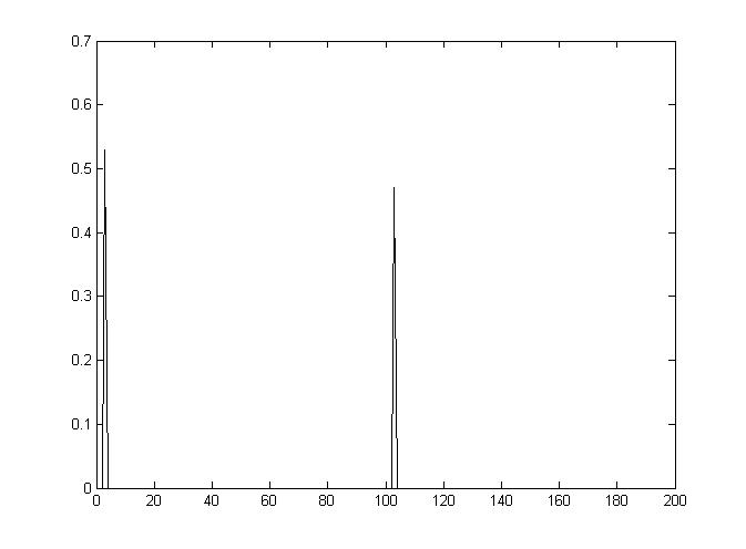
(a) Scarf model

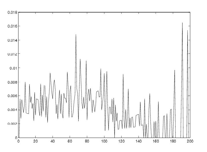
(b) LRO model

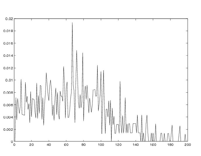
(c) LRO ($\hat{\mu},\hat{\sigma}^{2}$) model

Figure 1: Worst-case distributions

In Figure 1, the $x$-axis is the demand and the $y$-axis is the probability mass function over the demands. We can see that the worst-case distribution in the Scarf model is a two-point distribution (with positive mass at $3$ and $103$). However, a two-point distribution is not a realistic one, which means that Scarf’s approach might be guarding some overly conservative scenarios. In contrast, the worst-case distributions when we use LRO and LRO($\hat{\mu},\hat{\sigma}^{2}$) are much closer to the empirical data and look much more plausible. In particular, the LRO with mean and variance constraints results in a worst-case distribution closest to the empirical data among these three approaches.

The situation is different in the second case when the underlying distribution is an exponential distribution. In this case, Scarf’s solution is significantly worse than the LRO solutions. This is because it does not use the information that the data are skewed. In fact, it still only takes the mean and variance as the input. In contrast, the LRO and LRO($\hat{\mu},\hat{\sigma}^{2}$) adapt to the asymmetry of the data and only consider the distributions that are close to the empirical distribution.

In both cases, we observe that the LRO($\hat{\mu},\hat{\sigma}^{2}$) seems to work better. Indeed, we find that adding some constraints on $p$ regarding the mean/variance of the distribution usually helps the performance. This is because it helps to further concentrate the distribution set to those that have similar shape as the empirical distribution. Lastly, we find that the empirical distribution works well if we use the true distribution to evaluate the performance. However, it is not robust to potential deviations to the underlying distribution. As shown in the last column in Tables 1 and 2, when we allow the underlying distribution to change to some degree (within a 95% confidence range), the performance of the solution obtained by using the empirical distribution might be less than optimal.

4.2 Application 2: Portfolio Selection Problem

In this subsection, we apply the LRO model to the portfolio selection problem. In the portfolio selection problem, there are $d$ assets that are available to invest for the next day. The decision maker observes $N$ historical daily returns of the $d$ assets $\{\mbox{\boldmath$\xi$}_{i}\}_{i=1}^{N}$ where each $\mbox{\boldmath$\xi$}_{i}$ is a $d$-dimensional vector drawn from some underlying unknown distribution. In our case, we consider a certain support $\Omega$ of all possible returns, and the choice of $\Omega$ can be derived by using statistical models to calculate the boundaries of the possible returns. The decision in this problem is to make a portfolio selection $x$ in a feasible set $D$ (e.g., $D$ may contain some budget constraints) to maximize the expected return. We refer the readers to Luenberger [20] for a thorough review of the literature on this problem.

In this section, we demonstrate how to apply the LRO model to the portfolio selection problem and compare its performance to that of some other methods. First, we formulate the LRO model for the portfolio selection problem as follows:

$$\mbox{maximize}_{\mbox{\boldmath$x$}\in D} \mbox{min}_{\mbox{\boldmath$p$}} \sum_{i=1}^{N}p_{i}\cdot\mbox{\boldmath$\xi$}_{i}^{T}\mbox{\boldmath$x$}+\sum_{\sigma\in\Omega}p_{\sigma}\cdot\mbox{\boldmath$\xi$}_{\sigma}^{T}\mbox{\boldmath$x$}$$

s.t. $$\sum_{i=1}^{N}\log{p_{i}}\geq\gamma$$

$$\mbox{\boldmath$e$}^{T}\mbox{\boldmath$p$}=1,\mbox{ }\mbox{\boldmath$p$}\geq 0.$$

In (4.2), the first term in the objective function corresponds to the scenarios that have been observed in the data, while the second term corresponds to the unobserved scenarios (it will be an infinite sum if $\Omega$ has an infinite support). The first constraint is the likelihood constraint as we introduced in Section 2. For the ease of notation, we assume that each return profile occurs only once in the data, which is legitimate if we assume that the return is continuously distributed. The choice of $\Omega$ can either be discrete or continuous. In fact, as long as we can solve

$$g(\mbox{\boldmath$x$})=\min_{\mbox{ }\mbox{\boldmath$\xi$}\in\Omega}\mbox{\boldmath$\xi$}^{T}\mbox{\boldmath$x$}$$ (17)

efficiently for any $x$, the whole problem can be formulated as a convex program with polynomial size. To see that, we take the dual of the inner problem of (4.2) and combine it with the outer problem. We have that the entire problem can be written as one single optimization problem as follows:

$$\mbox{maximize}_{\mbox{\boldmath$x$},\mu,\lambda} \mu+\gamma\lambda+N\lambda-N\lambda\log{\lambda}+\lambda\sum_{i=1}^{N}\log(\mbox{\boldmath$\xi$}_{i}^{T}\mbox{\boldmath$x$}-\mu)$$

s.t. $$\mu\leq\mbox{\boldmath$\xi$}_{\sigma}^{T}\mbox{\boldmath$x$},\quad\forall\sigma\in\Omega$$

$$\lambda\geq 0,\quad\mbox{\boldmath$x$}\in D.$$

It appears that the first set of constraints could be of large size, however, if $g(\mbox{\boldmath$x$})$ defined in (17) can be solved efficiently, then this is effectively one single constraint. For example, if $\Omega=\{(r_{1},...,r_{d})|r_{i}\in[\underline{r}_{i},\bar{r}_{i}]\}$, then the constraint is equivalent to $\mu\leq\underline{\mbox{\boldmath$r$}}^{T}\mbox{\boldmath$x$}$. If $\Omega=\{(r_{1},...,r_{d})|||\mbox{\boldmath$r$}-\mbox{\boldmath$r$}_{0}||_{2}\leq\eta\}$, then the constraint is equivalent to $\mu\leq\mbox{\boldmath$r$}_{0}^{T}\mbox{\boldmath$x$}-\eta||\mbox{\boldmath$x$}||$, which is also convex.

Again, we can add any convex constraints of $p$ into (4.2) such as constraints on the moments of the return. Thus our model is quite flexible. Next we perform numerical tests using our model. We adopt the following setup (this setup is also used in other studies of the portfolio selection problem, see, e.g., Delage and Ye [13]):

• We gather the historical data of 30 assets from the S&P $500$ Index during the time period from 2001 to 2004. In each experiment, we choose four assets to focus on and the decision is to construct a portfolio using these four assets for each day during this period. We use the past 30 days’ data as the observed data in the LRO approach.

To select the $\gamma$ in (4.2), we still use the asymptotic result in Theorem 1. In particular, we choose the degree of freedom in the chi-square distribution to equal the number of historical observations. Although this is a heuristic choice, we find it works well in the numerical test. We compare our approach to the following three other approaches:

1. A naive approach in which each day, the stock with the highest past 30 days’ average daily return is chosen to be the sole stock in the portfolio. We call this approach the single stock (SS) approach.

2. An approach in which each stock is chosen with 1/4 weight (in terms of the capital size) for each day. We call this approach the equal weights (EQ) approach.

3. The distributionally robust approach with fixed mean and variance (see Popescu [26]), called the DRO approach.

We acknowledge that there are many other ways one can choose the portfolio and we do not intend to show that our approach is the best one for this problem. Instead, we aim to illustrate that the LRO approach gives a decent performance with some desired features.

In Table 3, we present the test results. The results are obtained using codes written in MATLAB 2010b. Some of the codes are borrowed from Delage and Ye [13]. We did $100$ experiments (each with four different stocks randomly chosen from the 30 to form the portfolio for each day), and the tested period covers 721 days.

Approach	# LRO outperforms	Average gain of LRO over	Std of returns
LRO	N/A	N/A	$2.3\%$
SS	65	$1.8\%$	$3.3\%$
EQ	60	$1.1\%$	$1.5\%$
DRO	58	$1.3\%$	$2.4\%$

Table 3: Test results for the portfolio selection problem

In Table 3, the numbers in the second column indicate that among the $100$ experiments, the number of times the overall return of the LRO approach outperforms the corresponding method. The numbers in the third column are the improvements of the average return of the LRO method over the corresponding model, and the numbers in the last column are the standard deviations of all daily returns of the portfolio constructed using each method. From Table 3, we observe that among the $100$ experiments, LRO outperforms all other tested methods in terms of the number of times it has a higher return, as well as the average overall return during the $721$ days. Also, it has a decent standard deviation of the daily returns. In particular, it has a much smaller standard deviation than the SS approach, and a comparable standard deviation to the DRO approach. To investigate further, when we look at the portfolios constructed by the LRO method, we find that $52\%$ of the time, it chooses a single stock to form the portfolio. And it chooses two stocks, three stocks and all four stocks in its solution for $39\%$, $8\%$ and $1\%$ of the times. Therefore, we find that LRO approach implicitly achieves diversification, which is a feature that is usually desired in such problems.

5 Conclusion

In this paper, we propose a new distributionally robust optimization framework, the likelihood robust optimization model. The model optimizes the worst-case expected value of a certain objective function where the worst-case distribution is chosen from the set of distributions that make the observed data achieve a certain level of likelihood. The proposed model is easily solvable and has strong statistical meanings. It avoids the over-conservatism of other robust models while protecting the decisions from reasonable deviations from the empirical data. We discuss two applications of our model. The numerical results show that our model might be appealing in several applications.

6 Acknowledgement

The authors thank Dongdong Ge and Zhisu Zhu for valuable insights and discussions. The authors also thank Erick Delage for insightful discussions and for sharing useful codes for the numerical experiments.

References

- [1] A. Ben-Tal, D. den Hertog, A. De Waegenaere, B. Melenberg, and G. Rennen. Robust solutions of optimization problems affected by uncertain probabilities. Management Science, 59(2):341–357, 2013.
- [2] A. Ben-Tal, L. El Ghaoui, and A. Nemirovski. Robust Optimization. Princeton Series in Applied Mathematics, 2009.
- [3] A. Ben-Tal and A. Nemirovski. Robust solutions of uncertain linear programs. Operations Research Letters, 25(1):1–13, 1999.
- [4] D. Bertsimas and A.Thiele. Robust and data-driven optimization: Modern decision-making under uncertainty. In Tutorial on Operations Research. INFORMS, 2006.
- [5] D. Bertsimas, D. Brown, and C. Caramanis. Theory and applications of robust optimization. SIAM Review, 53(3):464–501.
- [6] D. Bertsimas, V. Gupta, and N. Kallus. Data-driven robust optimization. 2013. Working paper.
- [7] D. Bertsimas and M. Sim. The price of robustness. Operations Research, 52(1):35–53, 2004.
- [8] D. Bertsimas and A. Thiele. A robust optimization approach to inventory theory. Operations Research, 54(1):150–168, 2006.
- [9] S. Boyd and L. Vandenberghe. Convex Optimization. Cambridge University Press, 2004.
- [10] G. Calafiore and L. El Ghaoui. On distributionally robust chance-constrained linear programs. Optimization Theory and Applications, 130(1):1–22, 2006.
- [11] X. Chen, M. Sim, and P. Sun. A robust optimization perspective on stochastic programming. Operations Research, 55(6):1058–1071, 2007.
- [12] E. Delage. Distributionally Robust Optimization in Context of Data-Driven Problem. PhD thesis, 2009.
- [13] E. Delage and Y. Ye. Distributionally robust optimization under moment uncertainty with application to data-driven problems. Operations Research, 58(3):595–612, 2008.
- [14] J. Dupaĉová. The minimax approach to stochastic programming and an illustrative application. Stochastics, 20(1):73–88, 1987.
- [15] G. Gallego and I. Moon. The distribution free newsboy problem: Review and extension. The Journal of the Operational Research Society, 44(8):825–834, 1993.
- [16] A. Gelman, J. Carlin, H. S. Stern, and D. B. Rubin. Bayesian Data Analysis. Chapman and Hall Press, 1995.
- [17] G. Iyengar. Robust dynamic programming. Mathematics of Operations Research, 30(2):257–280, 2005.
- [18] N. Johnson, S. Kotz, and N. Balakrishnan. Continuous Univariate Distributions, Vol. 1. Wiley Series in Probability and Statistics, 1994.
- [19] M. Khouja. The single period newsvendor problem: Literature review and suggestions for future research. Omega, 27:537–553, 1999.
- [20] D. Luenberger. Investment Science. Oxford University Press, 1997.
- [21] D. Mason and J. Schuenemeyer. A modified Kolmogorov-Smirnov test sensitive to tail alternatives. Annals of Statistics, 11(3):933–946, 1983.
- [22] A. Nilim and L. El Ghaoui. Robust control of Markov decision processes with uncertain transition matrices. Operations Research, 53(5):780–798, 2005.
- [23] A. Owen. Empirical Likelihood. Chapman and Hall Press, 2001.
- [24] L. Pardo. Statistical Inference Based on Divergence Measures. Chapman and Hall Press, 2005.
- [25] G. Perakis and G. Roels. Regret in the newsvendor model with partial information. Operations Research, 56(1):188–203, 2008.
- [26] I. Popescu. Robust mean-covariance solutions for stochastic optimization. Operations Research, 55(1):98–112, 2007.
- [27] H. Scarf. A min-max solution of an inventory problem. In K. Arrow, S. Karlin, and H. Scarf, editors, Studies in The Mathematical Theory of Inventory and Production, pages 201–209. Stanford University Press, 1958.
- [28] H. Scarf. Bayes solutions of the statistical inventory problem. Annal of Mathematical Statistics, 30(2):490–508, 1959.
- [29] A. Shapiro, D. Dentcheva, and A. Ruszczynski. Lectures on Stochastic Programming: Modeling and Theory. MPS-SIAM Series on Optimization, 2009.
- [30] A. Shapiro and A. J. Kleywegt. Minimax analysis of stochastic programs. Optimization Methods and Software, 17:523–542, 2002.
- [31] A. M-S. So, J. Zhang, and Y. Ye. Stochastic combinatorial optimization with controllable risk aversion level. Mathematics of Operations Research, 34(3):522–537, 2009.
- [32] L. Wassaman. All of Statistics: A Concise Course in Statistical Inference. Springer Texts in Statistics, 2009.
- [33] J. Yue, B. Chen, and M. Wang. Expected value of distribution information for the newsvendor problem. Operations Research, 54(6):1128–1136, 2006.
- [34] J. Ẑáĉková. On minimax solutions of stochastic linear programming problems. Ĉasopis pro Pêstování Matematiky, 91:423–430, 1966.
- [35] Z. Zhu, J. Zhang, and Y. Ye. Newsvendor optimization with limited distribution information. Optimization Methods and Software, 28(3):640–667, 2013.