Complex Network Approach to the Statistical Features of the Sunspot Series

Abstract

Complex network approaches have been recently developed as an alternative framework to study the statistical features of time-series data. We perform a visibility-graph analysis on both the daily and monthly sunspot series. Based on the data, we propose two ways to construct the network: one is from the original observable measurements and the other is from a negative-inverse-transformed series. The degree distribution of the derived networks for the strong maxima has clear non-Gaussian properties, while the degree distribution for minima is bimodal. The long-term variation of the cycles is reflected by hubs in the network which span relatively large time intervals. Based on standard network structural measures, we propose to characterize the long-term correlations by waiting times between two subsequent events. The persistence range of the solar cycles has been identified over 15 – 1000 days by a power-law regime with scaling exponent $\gamma=2.04$ of the occurrence time of the two subsequent and successive strong minima. In contrast, a persistent trend is not present in the maximal numbers, although maxima do have significant deviations from an exponential form. Our results suggest some new insights for evaluating existing models. The power-law regime suggested by the waiting times does indicate that there are some level of predictable patterns in the minima.

1 Introduction

S-Introduction Solar-cycle prediction, i.e. forecasting the amplitude and/or the epoch of an upcoming maximum is of great importance as solar activity has a fundamental impact on the medium-term weather conditions of the Earth, especially with increasing concern over the various climate change scenarios. However, predictions have been notoriously wayward in the past [Hathaway (2010), Pesnell (2012)]. There are basically two classes of methods for solar cycle predictions: empirical data-analysis-driven methods and methods based on dynamo models. Most successful methods in this regard can give reasonably accurate predictions only when a cycle is well advanced (e.g., three years after the minimum) or with the guidance from its past [Kurths and Ruzmaikin (1990), Hathaway, Wilson, and Reichmann (1994)]. Hence, these methods show very limited power in forecasting a cycle which has not yet started. The theoretical reproduction of a sunspot series by most current models shows convincingly the “illustrative nature” of the existing record [Petrovay (2010)]. However, they generally failed to predict the slow start of the present Cycle 24 [Solanki and Krivova (2011)]. One reason cited for this is the emergence of prolonged periods of extremely low activity. The existence of these periods of low activity brings a big challenge for solar-cycle prediction and reconstruction by the two classes of methods described above, and hence prompted the development of special ways to evaluate the appearance of these minima [Brajša et al. (2009)]. Moreover, there is increasing interest in the minima since they are known to provide insight for predicting the next maximum [Ramesh and Lakshmi (2012)].

Some earlier authors have both observed and made claims for the chaotic or fractal features of the observed cycles, but the true origin of such features has not yet been fully resolved. For instance, the Hurst exponent has been used as a measure of the long-term memory in time series [Mandelbrot and Wallis (1969), Ruzmaikin, Feynman, and Robinson (1994)] – an index of long-range dependence that can be often estimated by a rescaled range analysis. The majority of Hurst exponents reported so far for the sunspot numbers are well above $0.5$, indicating some level of predictability in the data. Nonethteless, it is not clear whether such predictability is due to an underlying chaotic mechanism or the presence of correlated changes due to the quasi-11-year cycle [Oliver and Ballester (1998), Pesnell (2012)]. It is the irregularity (including the wide variations in both amplitudes and cycle lengths) that makes the prediction of the next cycle maximum an interesting, challenging and, as yet, unsolved issue. In contrast to the 11-year cycle per se, we concentrate on the recently proposed hypothetical long-range memory mechanism on time scales shorter than the quasi-periodic 11-year cycle [Rypdal and Rypdal (2012)].

In this work, we provide a distinct perspective on the strong maximal activities and quiescent minima by means of the so-called visibility graph analysis. Such graphs (mathematica graphs, in the sense of networks) have recently emerged as one alternative to describe various statistical properties of complex systems. In addition to applying the standard method, we generalize the technique further – making it more suitable for studying the observational records of the solar cycles.

2 Data and Network Construction

S-Data Both the International Sunspot Number (ISN) and the sunspot area (SSA) series [SIDC-team (2011)] are used in this work, and we have obtained consistent conclusions in either case. The length of the data sets are summarized in Table tab:tspan. We perform a visibility-graph analysis using both monthly and daily sunspot series, which yields, respectively, month-to-month and day-to-day correlation patterns of the sunspot activities. Note that we depict the annual numbers only for graphical visualization and demonstration purposes (we use the annual numbers to demonstrate our method — the actual analysis is performed in daily and monthly data). We discuss the results with the ISN (in Figs. sn_sa_data, ts_deg_maxMin_cp) in the main text and illustrate the results for the SSA (in Figs. sa_nasa_data, ts_deg_maxMin_cpNASA) with notes in the captions. Moreover, we compare our findings based on observational records to the results obtained from data produced by simulations from computational models [Barnes, Tryon, and Sargent (1980), Mininni, Gómez, and Mindlin (2000)].

Table 1.: Temporal resolution and the length of the data sets. Values in parentheses are the number of points of each series. Note that the annual ISN is used only for graphical visualization purposes and to provide a reference time interval for models.tab:tspan

	ISN	SSA
Day	1 Jan 1849 – 31 Oct 2011	1 May 1874 – 31 Oct 2011
	(59473)	(50222)
Mon.	Jan 1849 – Oct 2011	May 1874 – Oct 2011
	(1944)	(1650)
Year	1700 – 2010	not used
	(311)

Recently a variety of methods have been proposed for studying time series from a complex networks viewpoint, providing us with many new and distinct statistical properties [Zhang and Small (2006), Xu, Zhang, and Small (2008), Marwan et al. (2009), Donner et al. (2010), Donner et al. (2011)]. In this work, we restrict ourselves to the concept of the visibility graph (VG), where individual observations are considered as vertices and edges are introduced whenever vertices are visible. More specifically, given a univariate time series $x(t_{i})_{i=1,\ldots,N}$, we construct the 0 – 1 binary adjacency matrix $A_{N\times N}$ of the network. The algorithm for deciding non-zero entries of $A_{i,j}$ considers two time points $t_{i}$ and $t_{j}$ as being mutually connected vertices of the associated VG if the following criterion

$$\ilabel{vis_{c}ond}\frac{x(t_{i})-x(t_{k})}{t_{k}-t_{i}}>\frac{x(t_{i})-x(t_{j})}{t_{j}-t_{i}}$$ (1)

is fulfilled for all time points $t_{k}$ with $t_{i}<t_{k}<t_{j}$ [Lacasa et al. (2008)]. Therefore, the edges of the network take into account the temporal information explicitly. By default, two consecutive observations are connected and the graph forms a completely connected component without disjoint subgraphs. Furthermore, the VG is known to be robust to noise and not affected by choice of algorithmic parameters – most other methods of constructing complex networks from time series data are dependent on the choice of some parameters (e.g. the threshold $\varepsilon$ of recurrence networks, see more details in [Donner et al. (2010)]). While the inclusion of these parameters makes these alternative schemes more complicated, they do gain the power to reconstruct (with sufficient data) the underlying dynamical system. For the current discussion we prefer the simplicity of the visibility graph. The VG approach is particularly interesting for certain stochastic processes where the statistical properties of the resulting network can be directly related with the fractal properties of the time series [Lacasa et al. (2009), Elsner, Jagger, and Fogarty (2009), Nuñez et al. (2012), Donner and Donges (2012), Donges, Donner, and Kurths (2013)].

Figure visi_intro illustrates an example of how we construct a VG for the sunspot time series. It is well known that the solar cycle has an approximately 11-year period, which shows that most of the temporal points of the decreasing phase of one solar cycle are connected to those points of the increasing phase of the next cycle (Figure visi_intro(a)). Therefore, the network is clustered into communities, each of which mainly consists of the temporal information of two subsequent solar cycles (Figure visi_intro(b)). When the sunspot number reaches a stronger but more infrequent extreme maximum, we have inter-community connections, since they have a better visibility contact with more neighbors than other time points – hence, forming hubs in the graph. The inter-community connections extend over several consecutive solar cycles encompassing the temporal cycle-to-cycle information.

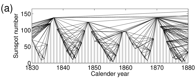
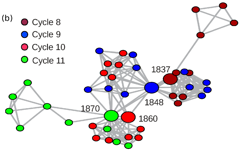
Figure 1.: The procedure to construct a VG. Note that an enlargement of the particular time span of the annual data is used here only for visualization purposes, while the analysis performed throughout is based on both monthly and daily series. (A) sunspot numbers in gray bar plot, where two time points fulfilling the visibility condition are connected by a line; (B) complex network representation, one network cluster usually includes time points of two subsequent solar cycles; (C) degree sequences of the original series $x(t_{i})$ (open circles) and the negatively inverted series $-x(t_{i})$ (filled circles), respectively.visi˙intro

Depending on various notions of “importance” of a vertex with respect to the entire network, various centrality measures have been proposed to quantify the structural characteristics of a network (c.f. [Newman (2003)]). Recent work on VGs has mainly concentrated on the properties of the degree and its probability distribution $p(k)$, where degree $k$ measures the number of direct connections that a randomly chosen vertex $i$ has, namely, $k_{i}=\sum_{j}A_{i,j}$. The degree sequence reflects the maximal visibility of the corresponding observation in comparison with its neighbors in the time series (Figure visi_intro(c)). Based on the variation of the degree sequence $k_{i}$, we consider $1837$, $1848$, $1860$, and $1870$ as hubs of the network, which can be used to identify the approximately 11-year cycle reasonably well (Figure visi_intro(b)).

Furthermore in the case of sunspot time series, one is often required to investigate what contributions local minimum values make to the network – something that has been largely overlooked by the traditional VGs. One simple solution is to study the negatively inverted counterpart of the original time series, namely, $-x(t_{i})$, which quantifies the properties of the local minima. We use $k_{-x}$ and $p(k_{-x})$ to denote the case of $-x(t_{i})$. Here, we remark that this simple inversion of the time series allows us to create an entirely different complex network – this is because the VG algorithm itself is extremely simple and does not attempt to reconstruct an underlying dynamical system. As shown in Figure visi_intro(c), $k_{-x}$ captures the variation of the local minima rather well. We will use this technique later to understand the long-term behavior of strong minima of the solar cycles.

The degree distribution $p(k)$ is defined to be the fraction of nodes in the network with degree $k$. Thus if there are $N$ nodes in total in a network and $n_{k}$ of them have degree $k$, we have $p(k)=n_{k}/N$. For many networks from various origins, $p(k)$ has been observed to follow a power-law behavior: $p(k)\sim k^{-\gamma}$. In the case of VGs, $p(k)$ is related to the dynamical properties of the underlying processes [Lacasa et al. (2008)]. More specifically, for a periodic signal, $p(k)$ consists of several distinct degrees indicating the regular structure of the series; for white noise, $p(k)$ has an exponential form; for fractal processes, the resulting VGs often have power law distributions $p(k)\sim k^{-\gamma}$ with the exponent $\gamma$ being related to the Hurst exponent $H$ of the underlying time series [Lacasa et al. (2009)]. It is worth pointing out that when one seeks to estimate the exponent $\gamma$ it is often better to employ the cumulative probability distribution $F(k)=\sum_{k>k_{0}}p(k)$ so as to have a more robust statistical fit.

Estimating the exponent $\gamma$ of the hypothetical power law model for the degree sequence of VG can be done rather straightforwardly, but, the statistical uncertainties resulting from the observability of sunspots are a challenge for reliable interpretation. Meanwhile, fitting a power law to empirical data and assessing the accuracy of the exponent $\gamma$ is a complicated issue. In general, there are many examples which had been claimed to have power laws but turn out not to be statistically justifiable. We apply the recipe of Clauset2009 to analyze the hypothetical power-law distributed data, namely, (i) estimating the scaling parameter $\gamma$ by the maximum likelihood (ii) generating a $p$-value that quantifies the plausibility of the hypothesis by the Kolmogorov – Smirnov statistic.

Aside from the aforementioned degree $k_{i}$ and degree distribution $p(k)$, in the Appendix sapp:bet, some alternative higher order network measures are suggested which may be applied to uncover deeper dynamical properties of the time series from the VG.

3 Results

Figure sn_sa_data(a,b) show the degree distributions $p(k)$ of the VGs derived from the ISN $x(t_{i})$ with heavy-tails corresponding to hubs of the graph, which clearly deviates from Gaussian properties. In contrast, $p(k_{-x})$ of the negatively inverted sunspot series $-x(t_{i})$ shows a completely different distribution, consisting of a bimodal property (Figure sn_sa_datac,d), extra large degrees are at least two orders of magnitude larger than most of the vertices (Figure sn_sa_data(d)).

Figure 2.: Degree distribution $p(k)$ of VGs from monthly (A,C) and daily data (B,D). (A,B) is for $x(t_{i})$, and (C,D) $-x(t_{i})$. Upper insets of all plots are $p(k)$ in linear scale, while lower inset of (A,B) shows cumulative distribution $F(k)$ in double logarithmic scale, where a straight line is expected if $F(k)$ would follow a power law $\sim k^{-(\gamma-1)}$. In (A,B) $\gamma$s could be suspected to be in the range $[2.32,2.64]$, while a fit to the first part of $p(k_{-x})$ yields that the slope of dashed line in (C) is 1.79, and that of (D) is 3.61, but all $p$-values are $0$, rejecting the hypothetical power laws.sn˙sa˙data

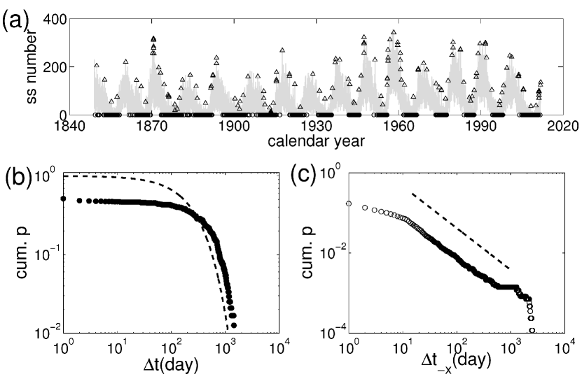
Figure 3.: (A) Time points annotated by vertices with large degrees. Triangles (strong maxima) correspond to the VG constructed from the original series $x(t_{i})$, while circles (strong minima) are that of the VG from $-x(t_{i})$. (B, C) Cumulative probability distribution of the time intervals between subsequent strong maxima (B), and minima (C). A cumulative exponential distribution is plotted as a dashed line in (B), while the dashed line in (C) is a linear fit with slope being equal to $\gamma-1=1.04$. The corresponding $p$-value of (C) is $0.45$, indicating that the power law is a plausible hypothesis for the waiting times of strong minima. ts˙deg˙maxMin˙cp

Since well-defined scaling regimes are absent in either $p(k)$ or $p(k_{-x})$ (nor do they appear in the cumulative distributions as shown in the insets, see captions of Figure sn_sa_data for details of the statistical tests which we apply), we may reject the hypothetical power laws – in contrast to what has been reported in other contexts [Lacasa et al. (2008), Lacasa et al. (2009)].

In the context of studying grand maxima/minima over (multi-)millennial timescale using some particular indirect proxy time series, the main idea lies in an appropriately chosen threshold, excursions above which are defined as grand maxima, respectively, below which are defined as grand minima [Voss, Kurths, and Schwarz (1996), Usoskin, Solanki, and Kovaltsov (2007)]. In this work, we use a similar concept but here in terms of degrees of the corresponding VG. We define a strong maximum if its degree $k$ is larger than $100$ (Figure sn_sa_dataa,b), a strong minimum if its degree $k_{-x}$ is over $1000$ (Figure sn_sa_datac,d). Note that, in general, our definition of strong maxima/minima coincides neither with the local maximal/minimal sunspot profiles since degree $k$ takes into account the longer term inter-cycle variations nor with those defined for an individual cycle. Our definition avoids the choice of maximum/minimum for one cycle, which suffers from moving-average effects (e.g., [Hathaway (2010)]). In contrast, our results below are robust with respect to the choice of the threshold degrees, especially in the case of the definition of strong minima, since large degrees are very well separated from others. The gray line in Figure ts_deg_maxMin_cp(a) shows the sunspot numbers overlaid by the maxima/minima identified by the large degrees. We find that the positions of strong maxima are substantially homogeneously distributed over the time domain, while that of the strong minima are much more clustered in the time axis although irregularly (Figure ts_deg_maxMin_cp(a)). We emphasize that the clustering behavior of the strong minima on the time axis as shown in Figure ts_deg_maxMin_cp(a) and Figure ts_deg_maxMin_cpNASA(a) does not change if threshold degrees are varied in the interval of (200, 8000) to define strong minima, i.e., $k>7000$, as shown in Figure ts_degK7000(a,b). Therefore, the bimodality as observed in Figure sn_sa_data(c,d) and Figure sa_nasa_data(c,d) are not due to the finite size effects of time series.

The hidden regularity of the time positions of maxima/minima can be further characterized by the waiting time distribution [Usoskin, Solanki, and Kovaltsov (2007)]: the interval between two successive events is called the waiting-time. The statistical distribution of waiting-time intervals reflects the nature of a process which produces the studied events. For instance, an exponential distribution is an indicator of a random memoryless process, where the behavior of a system does not depend on its preceding states on both short or long time scales. Any significant deviation from an exponential law suggests that the underlying event occurrence process has a certain level of temporal dependency. One representative of the large class of non-exponential distributions is the power laws, which have been observed in many different contexts, ranging from the energy accumulation and release property of earthquakes to social contacting patterns of humans [Wu et al. (2010)].

In the framework of VGs, the possible long temporal correlations are captured by edges that connect different communities (the increasing and decreasing phases of one solar cycle belong to two temporal consecutive clusters). As shown in Figure ts_deg_maxMin_cp(b), the distribution of the waiting time between two subsequent maxima sunspot deviates significantly from an exponential function, although the tail part could be an indicator of an exponential form. In contrast, we show in Figure ts_deg_maxMin_cp(c) that the waiting times between subsequent strong minima have a heavy-tail distribution where the exponent $\gamma\approx 2.04$ is estimated in the scaling regime. This suggests that the process of the strong minima has a positive long term correlation, which might be well developed over the time between 15 – 1000 days where a power-law fit is taken. Waiting time intervals outside this range are due to either noise effects on shorter scales or the finite length of observations on longer time scales. Again, the power law regimes identified by the waiting time distributions are robust for various threshold degree values in the interval of (200, 8000) (for instance, the case of $k>7000$ is shown in Figure ts_degK7000(c,d)).

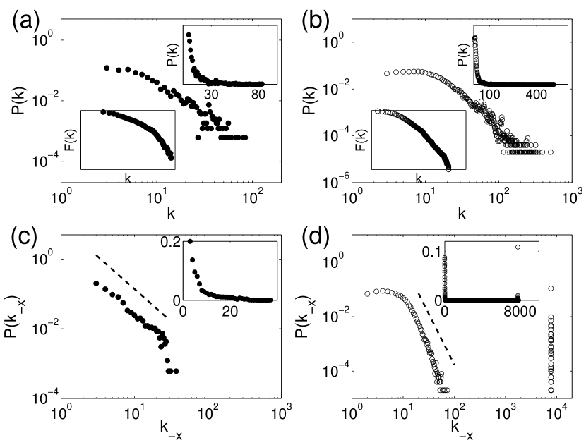
Figure 4.: For the SSA data. Degree distribution $p(k)$ of VGs from monthly (A,C) and daily data (B,D). (A,B) is for $x(t_{i})$, and (C,D) $-x(t_{i})$. Upper insets of all plots are $p(k)$ in linear scale, while lower inset of (A,B) shows cumulative distribution $F(k)$ in double logarithmic scale, where a straight line is expected if $F(k)$ would follow a power law $\sim k^{-(\gamma-1)}$. In (C,D), $\gamma$s could be fit by dashed lines (slopes: C, $1.86$; D, $3.73$ respectively), but all $p$-values are $0$ rejecting the hypothetical power laws.sa˙nasa˙data

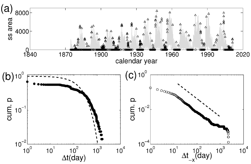
Figure 5.: For the SSA data. (A) Time points annotated by vertices with large degrees. Triangles (strong maxima) correspond to the VG constructed from the original series $x(t_{i})$, while circles (strong minima) are that of the VG from $-x(t_{i})$. (B, C) Cumulative probability distribution of the time intervals between subsequent strong maxima (B), and minima (C). A cumulative exponential distribution is plotted as a dashed line in (B), while the dashed line in (C) is a linear fit with slope being equal to $\gamma-1=1.04$. The corresponding $p$-value of (C) is $0.78$, indicating that the power law is a plausible hypothesis for the waiting times of strong minima.ts˙deg˙maxMin˙cpNASA

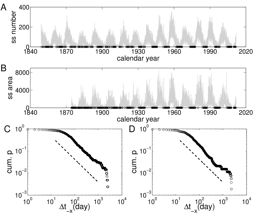
Figure 6.: Time points annotated by vertices with strong minima, which are defined by network degrees ($k>7000$) of VGs reconstructed from negatively inversed series. (A) ISN, and (B) SSA. Cumulative probability distribution of the time intervals between subsequent strong minima, (C) ISN, and (D) SSA. The dashed lines in (C, D) are linear fits which are obtained in the same way as shown in Figs. ts_deg_maxMin_cpC, ts_deg_maxMin_cpNASAC, respectively. ts˙degK7000

4 Discussion

In contrast to the computations described above with observational data, we now demonstrate the inadequacy of two models of solar cycles. By applying the VG methods to model simulations we demonstrate that the observed data has, according to the complex network perspective, features absent in the models. We first choose a rather simple yet stochastic model which describes the temporal complexity of the problem, the Barnes model [Barnes, Tryon, and Sargent (1980)], consisting of an autoregressive moving average ARMA(2, 2) model with a nonlinear transformation

$$z_{i} = \alpha_{1}z_{i-1}+\alpha_{2}z_{i-2}+a_{i}-\beta_{1}a_{i-1}-\beta_{2}a_{i-2},$$ (2)

$$s_{i} = z_{i}^{2}+\gamma(z_{i}^{2}-z_{i-1}^{2})^{2},$$ (3)

where $\alpha_{1}=1.90693$, $\alpha_{2}=-0.98751$, $\beta_{1}=0.78512$, $\beta_{2}=-0.40662$, $\gamma=0.03$ and $a_{i}$ are identically independent distributed Gaussian random variables with zero mean, and standard deviation SD = 0.4. The second model is a stochastic relaxation Van der Pol oscillator which is obtained from a spatial truncation of the dynamo equations [Mininni, Gómez, and Mindlin (2000)]. The equations read

$$\dot{x} = y,$$ (4)

$$\dot{y} = -\omega^{2}x-\mu y[3(\xi_{0}+r\xi_{s})x^{2}-1],$$ (5)

where $\omega=0.2993$, $\mu=0.2044$, $\xi=0.0102$, $\xi_{s}$ is Gaussian noise with zero mean and SD = 1, and $r$ is adjustable but often chosen to be $0.02$. The variable $x$ is associated with the mean toroidal magnetic field, and therefore the sunspot number is considered to be proportional to $x^{2}$, which prompts us to construct VGs from $x^{2}$ ($-x^{2}$ respectively). Both models reproduce the rapid growth in the increasing phase and slow decay in the decreasing phase of the activity cycles adequately. For the truncated model of the dynamo equations, a statistical significant correlation between instantaneous amplitude and frequency has been established, while the Barnes model shows virtually no correlation [Mininni, Gomez, and Mindlin (2002)], which are generally termed as the Waldmeier effect.

From both models, we generate $10,000$ independent realizations, each of them has a one month temporal resolution and the same time span as we have for the observations (namely, over $300$ years). We then construct VGs from both $x_{t_{i}}$ and $-x_{t_{i}}$ from each realization in the same way as we processed for the original observation. As shown in Figure barnes_mininni_model, neither $p(k)$ can mimic the heavy tails of the distributions we observed in Figure sn_sa_data(a,b), nor $p(k_{-x})$ can capture the bimodality of the large degrees for strong minima as we have observed in the case of observational raw records in Figure sn_sa_data(c,d). This does not occur even if the parameter $r$ of the second model is adjusted (Figure barnes_mininni_model(c,d)). One reason for the absence of the bimodality of $p(k)$ in the nonlinear-oscillator model is the fact that the model was designed to reproduce smoothed sunspot-number time series. The often-used 13-month running-average method in the literature is known to suppress the maximum/minimum amplitudes of the series [Hathaway (2010)]. Therefore, the visibility condition for each time point is changed if the 13-month smoothing technique is applied to the original data. We show the degree distribution $p(k)$ of VGs reconstructed from smoothed ISN series in Appendix (Figure pdf_smooth(b)), where the bimodality is absent.

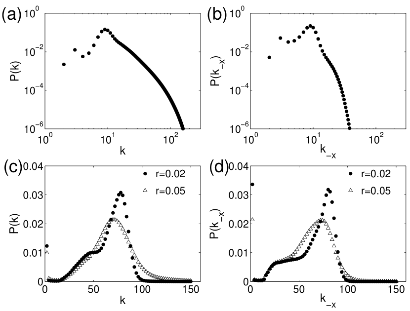
Figure 7.: Degree distribution $p(k)$ of VGs constructed from: (A, B) $x(t_{i})$ and $-x(t_{i})$ of Barnes’ model, and (C, D) $x^{2}$ and $-x^{2}$ of Mininni’s model. All $p(k)$ and $p(k_{-x})$ are estimated by an average over $10,000$ independent realizations using a kernel smoother. In (C, D) $r=0.02$ (filled circles), $r=0.05$ (open triangles).barnes˙mininni˙model

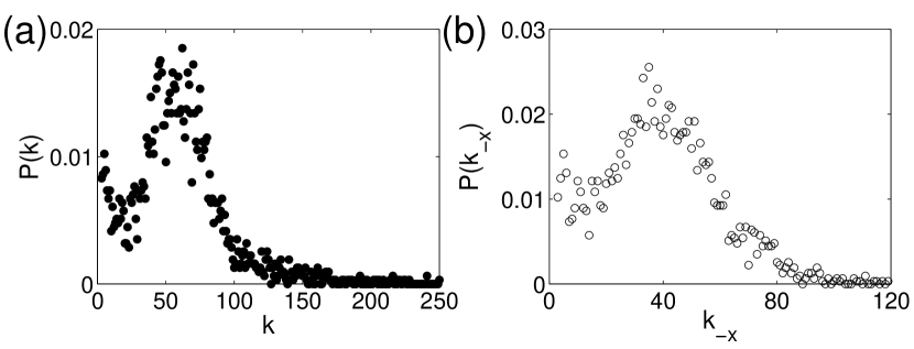
Figure 8.: Degree distribution $p(k)$ of VGs reconstructed from smoothed monthly ISN data. (A) is for $x(t_{i})$, and (B) $-x(t_{i})$. pdf˙smooth

As shown in Figure barnes_mininni_model, strong maxima/minima are not well separated. Consequently we are prevented from identifying unique waiting time sequences. The corresponding analysis then depends significantly on the choice of threshold degrees.

Dynamo theory provides several hints that might explain the features observed in the long-term evolution of the solar activity. The two theoretical models tested in this work can reproduce qualitative features of the system reasonably well, however, within the context performed in this study, cannot yield a complete and conclusive rendition of the statistical properties of $p(k)$. The power-law regimes obtained from waiting time sequences suggest that the interaction patterns for two subsequent minima can be much more complicated than what has been previously described as the instantaneous amplitudes – frequencies correlation using rather simple models [Paluš and Novotná (1999), Mininni, Gomez, and Mindlin (2002)].

5 Conclusions

In this work, we apply a recently proposed network approach, namely the visibility graph, to disclose the intricate dynamical behavior of both strong maximal and minimal sunspot numbers with observational records. More specifically, we show that:

1. There is a strong degree of memory af the time scale of 15 – 1000 days in the occurrence of low-activity episodes, observed as clusters of inactive days. The identified persistence time scale of the strong minima agrees with the recently proposed hypothetical long range memory on time scales shorter than the 11-year cycle [Rypdal and Rypdal (2012)].

2. The occurrence of high activity episodes is nearly random, i.e. strong active regions appear more or less independently of each other. The distinctive long-term correlations of the strong maxima and strong minima are reflected by the structural asymmetries of the degree distributions $p(k)$ of the respective VGs.

3. There is no evidence for a long term inter-cycle memory. This is in agreement with the present paradigm based on alternative methods (see, e.g., reviews by [Petrovay (2010), Usoskin (2013)]), and provides an observational constraint for solar-activity models.

Since the long term intra-cycle memory is relatively easy to establish but inter-cycle memory remains largely unclear, therefore we propose that our results could be used for evaluating models for solar activity at this time scale because they reflect important properties that are not included in other measures reported in the literature.

From the methodological perspective, we propose an interesting generalization for the construction of VGs from the negatively-inverted time series. This has been seen, via our analysis of sunspot observations, to show complementary aspects of the original series. Note that the negatively-inverse transformation is crucial for understanding when asymmetry is preserved in the time series. Therefore, it is worth analyzing the dependence of the resulted VGs on an arbitrary monotonic nonlinear transformation. Furthermore, as presented in Appendix sapp:cor, a systematic investigation of the general conclusion as to whether large sampled points correspond to hubs of VGs will be a subject of future work – especially in the presence of cyclicity and asymmetry.

It is worth stressing that we construct VGs directly based on the raw sunspot series without any preprocessing. Many researchers prefer to base their studies on some kind of transformed series since most common methods of data analysis in the literature rely on the assumption that the solar activity follows Gaussian statistics [Pesnell (2012)]. It is certain that the conclusions will then show some deviations depending on the parameters chosen for the preprocessing. The pronounced peaked and asymmetrical sunspot-cycle profiles prompt one to develop techniques such that the possible bias due to the unavoidable choice of parameters should be minimized. The complex network perspective offered by VG analysis has the clear advantage of being independent of any priori parameter selection.

The procedure for network analysis outlined here can be directly applied to other solar activity indicators, for instance, the total solar irradiance and the solar – flare index. We compared our results to two rather empirical models and showed that the distinctive correlation patterns of maximal and minimal sunspots are currently absent from these two models. Using our analysis for more refined dynamo-based models (e.g. [Charbonneau (2010)]) would be straightforward. Certainly, further work on this line of research will examine any differences given by the particular quantity and strengthen the understanding of the hypothetical long-range memory process of the solar activity from a much broader overview.

This work was partially supported by the German BMBF (projects PROGRESS), the National Natural Science Foundation of China (Grant No. 11135001), and the Hong Kong Polytechnic University Postdoctoral Fellowship. MS is supported by an Australian Research Council Future Fellowship (FT110100896).

Appendix A Graph Visualization of Degree $k_{i}$ and Betweenness Centrality $b_{i}$

sapp:bet Besides the fact that the maximal sunspot numbers are identified as hubs of VGs by the degree sequence $k_{i}$, convincing links between further network-theoretic measures and distinct dynamic properties can provide some additional interesting understanding for the time series [Donner and Donges (2012)]. In this study, we provide a graphical visualization on the relationship between degree $k_{i}$ and node betweenness centrality $b_{i}$, which characterizes the node’s ability to transport information from one place to another along the shortest path.

Using the annual ISN as a graphical illustration, here only the relationship between some relatively large degrees ($k_{i}>15$) and betweenness centrality values ($b_{i}>0.2$) is highlighted in Figure year_sspnDegBet for the entire series available. For instance in the annual series, time points $1778$, $1789$, $1837$, $1870$, $1947$, $1957$, and $1989$ are all identified simultaneously as large degrees and high betweenness, indicating strong positive correlations.

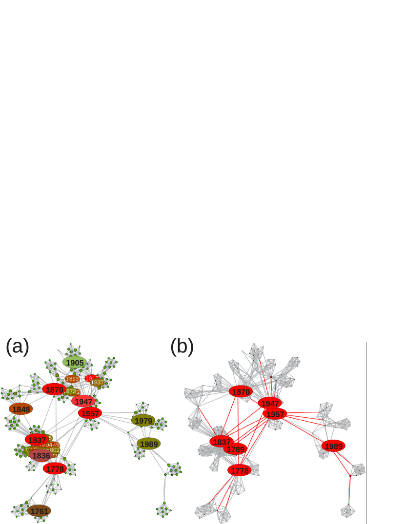
Figure 9.: Network representations of the VG constructed from the annual sunspot numbers of the entire series. Highlighted visible nodes are: (A) large degrees ($k_{i}>15$), and (B) high betweenness centrality ($b_{i}>0.2$). year˙sspnDegBet

Certainly many other measures can be directly applied to the sunspot numbers, however, providing the appropriate (quantitative) interpretations of the results in terms of the particular underlying geophysical mechanisms remains a challenging task and is largely open for future work. Note that there is in general a strong interdependence between these different network structural quantities.

Appendix B Correlation between $k_{i}$ and $x_{i}$

sapp:cor A general rule of understanding the scale-free property of the degree distribution of complex networks is the effects of a very few hubs having a large amount of connections. In the particular case of VGs, hubs are related to maxima of the time series since they have better visibility contact with more vertices than other sampled points. However, this result can not be generalized to all situations, for instance, it is easy to generate a time series such that its maxima are not always mapped to hubs in the VGs.

One simple way to better explore this correlation is to use scatter plots between the degree sequence and the sunspot time series. As we show in Figure deg_ts_rhoB, the Spearman correlation coefficients $\rho$ as very small (still significantly larger than zero) in the case of VGs reconstructed from the original time series. This provides an important cautionary note on the interpretation of hubs of VGs by local maximal values of the sunspot numbers. On the contrary if the network is reconstructed from $-x$, hubs of VGs could be better interpreted by local minimal values of the sunspot data since the correlations become larger. These results hold for both the ISN and SSA series (Figure deg_ts_rhoG). One reason for the lack of strong correlation between the degree $k_{i}$ and $x_{i}$ is because of the (quasi-)cyclicity of the particular time series, which has a similar effect as the Conway series [Lacasa et al. (2008)]. It is this concave behavior over the time axis (although quasi-periodic from cycle to cycle) that prevents the local maxima from having highly connected vertices. It remains unclear how local maxima of a time series are mapped to hubs of VGs – we defer this topic for future work especially in the presence of cyclicity. This situation becomes even more challenging if some sort of asymmetric property is preserved in the data, as we have found for the sunspot series.

Figure 10.: Scatter plot of the degree sequence $k_{i}$ – $x_{i}$ for VG constructed from ISN series based on (A) monthly and (B) daily data respectively. Spearman $\rho$ is indicated. (C, D) are based on the VGs constructed from negatively inverted series $-x_{i}$. deg˙ts˙rhoB

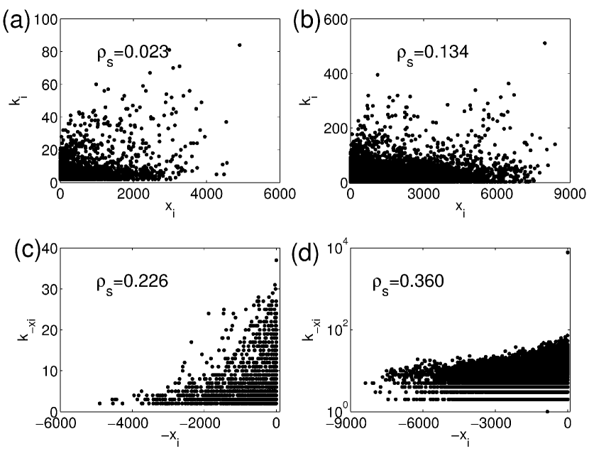
Figure 11.: Scatter plot of the degree sequence $k_{i}$ – $x_{i}$ for VG constructed from SSA series based on (A) monthly and (B) daily data respectively. Spearman $\rho$ is indicated. (C, D) are based on the VGs constructed from negatively inverted series $-x_{i}$.deg˙ts˙rhoG

References

- Barnes, Tryon, and Sargent (1980) Barnes, J.A., Tryon, P.V., Sargent, H.H. III: 1980, Sunspot cycle simulation using random noise. In: Pepin, R.O., Eddy, J.A., Merrill, R.B. (eds.) The Ancient Sun: Fossil Record in the Earth, Moon and Meteorites, Pergamon Press, New York and Oxford, 159 – 163.
- Brajša et al. (2009) Brajša, R., Wöhl, H., Hanslmeier, A., Verbanac, G., Ruždjak, D., Cliver, E., Svalgaard, L., Roth, M.: 2009, On solar cycle predictions and reconstructions. Astron. Astrophys. 496, 855 – 861. doi:10.1051/0004-6361:200810862.
- Charbonneau (2010) Charbonneau, P.: 2010, Dynamo models of the solar cycle. Living Rev. Solar Phys. 7(3). doi:10.12942/lrsp-2010-3.
- Clauset, Shalizi, and Newman (2009) Clauset, A., Shalizi, C.R., Newman, M.E.J.: 2009, Power-law distributions in empirical data. SIAM Rev. 51(4), 661 – 703.
- Donges, Donner, and Kurths (2013) Donges, J., Donner, R., Kurths, J.: 2013, Testing time series irreversibility using complex network methods. Europhys. Lett. 102(1), 10004.
- Donner and Donges (2012) Donner, R.V., Donges, J.F.: 2012, Visibility graph analysis of geophysical time series: Potentials and possible pitfalls. Acta Geophys. 60, 589 – 623.
- Donner et al. (2010) Donner, R.V., Zou, Y., Donges, J.F., Marwan, N., Kurths, J.: 2010, Recurrence networks – A novel paradigm for nonlinear time series analysis. New J. Phys. 12(3), 033025.
- Donner et al. (2011) Donner, R.V., Small, M., Donges, J.F., Marwan, N., Zou, Y., Xiang, R., Kurths, J.: 2011, Recurrence-based time series analysis by means of complex network methods. Int. J. Bifurcation Chaos 21(4), 1019 – 1046.
- Elsner, Jagger, and Fogarty (2009) Elsner, J.B., Jagger, T.H., Fogarty, E.A.: 2009, Visibility network of united states hurricanes. Geophys. Res. Lett. 36(16), L16702.
- Hathaway (2010) Hathaway, D.H.: 2010, The solar cycle. Living Rev. Solar Phys. 7, 1. doi:10.12942/lrsp-2010-1.
- Hathaway, Wilson, and Reichmann (1994) Hathaway, D., Wilson, R., Reichmann, E.: 1994, The shape of the sunspot cycle. Solar Phys. 151, 177 – 190. doi:10.1007/BF00654090.
- Kurths and Ruzmaikin (1990) Kurths, J., Ruzmaikin, A.A.: 1990, On forecasting the sunspot numbers. Solar Physics 126(2), 407 – 410. doi:10.1007/BF00153060.
- Lacasa et al. (2008) Lacasa, L., Luque, B., Ballesteros, F., Luque, J., Nuño, J.C.: 2008, From time series to complex networks: The visibility graph. Proc. Nat. Acad. Sci. USA 105(13), 4972 – 4975.
- Lacasa et al. (2009) Lacasa, L., Luque, B., Luque, J., Nuno, J.C.: 2009, The visibility graph: A new method for estimating the Hurst exponent of fractional Brownian motion. Europhys. Lett. 86(3), 30001.
- Mandelbrot and Wallis (1969) Mandelbrot, B.B., Wallis, J.R.: 1969, Some long-run properties of geophysical records. Water Resour. Res. 5(2), 321 – 340.
- Marwan et al. (2009) Marwan, N., Donges, J.F., Zou, Y., Donner, R.V., Kurths, J.: 2009, Complex network approach for recurrence analysis of time series. Phys. Lett. A 373(46), 4246 – 4254.
- Mininni, Gómez, and Mindlin (2000) Mininni, P.D., Gómez, D.O., Mindlin, G.B.: 2000, Stochastic Relaxation Oscillator Model for the Solar Cycle. Phys. Rev. Lett. 85, 5476 – 5479.
- Mininni, Gomez, and Mindlin (2002) Mininni, P.D., Gomez, D.O., Mindlin, G.B.: 2002, Instantaneous phase and amplitude correlation in the solar cycle. Solar Physics 208(1), 167 – 179. doi:10.1023/A:1019658530185.
- Newman (2003) Newman, M.E.J.: 2003, The structure and function of complex networks. SIAM Rev. 45(2), 167 – 256.
- Nuñez et al. (2012) Nuñez, A.M., Lacasa, L., Gomez, J.P., Luque, B.: 2012, Visibility algorithms: A short review. In: Zhang, Y. (ed.) New Frontiers in Graph Theory, InTech, Open Access Book, 119 – 152. doi:10.5772/34810.
- Oliver and Ballester (1998) Oliver, R., Ballester, J.L.: 1998, Is there memory in solar activity? Phys. Rev. E 58, 5650 – 5654.
- Paluš and Novotná (1999) Paluš, M., Novotná, D.: 1999, Sunspot cycle: A driven nonlinear oscillator? Phys. Rev. Lett. 83, 3406 – 3409.
- Pesnell (2012) Pesnell, W.D.: 2012, Solar cycle predictions (invited review). Solar Physics 281(1), 507 – 532. doi:10.1007/s11207-012-9997-5.
- Petrovay (2010) Petrovay, K.: 2010, Solar cycle prediction. Living Rev. Solar Phys. 7, 6. doi:10.12942/lrsp-2010-6.
- Ramesh and Lakshmi (2012) Ramesh, K.B., Lakshmi, N.B.: 2012, The amplitude of sunspot minimum as a favorable precursor for the prediction of the amplitude of the next solar maximum and the limit of the waldmeier effect. Solar Phys. 276, 395 – 406. doi:10.1007/s11207-011-9866-7.
- Ruzmaikin, Feynman, and Robinson (1994) Ruzmaikin, A., Feynman, J., Robinson, P.: 1994, Long-term persistence of solar activity. Solar Phys. 149, 395 – 403.
- Rypdal and Rypdal (2012) Rypdal, M., Rypdal, K.: 2012, Is there long-range memory in solar activity on timescales shorter than the sunspot period? J. Geophys. Res. 117, A04103.
- SIDC-team (2011) SIDC-team: 2011, The International Sunspot Number & Sunspot Area Data. Monthly Report on the International Sunspot Number, http://www.sidc.be/sunspot-data/, Royal Observatory Greenwich, http://solarscience.msfc.nasa.gov/greenwch.shtml/.
- Solanki and Krivova (2011) Solanki, S.K., Krivova, N.A.: 2011, Analyzing solar cycles. Science 334(6058), 916 – 917.
- Usoskin (2013) Usoskin, I.G.: 2013, A history of solar activity over millennia. Living Rev. Solar Phys. 10, 1. doi:10.12942/lrsp-2013-1.
- Usoskin, Solanki, and Kovaltsov (2007) Usoskin, I.G., Solanki, S.K., Kovaltsov, G.A.: 2007, Grand minima and maxima of solar activity: new observational constraints. Astron. Astrophys. 471, 301 – 309.
- Voss, Kurths, and Schwarz (1996) Voss, H., Kurths, J., Schwarz, U.: 1996, Reconstruction of grand minima of solar activity from C data: Linear and nonlinear signal analysis. J. Geophys. Res. 101(A7), 15637 – 15643.
- Wu et al. (2010) Wu, Y., Zhou, C.S., Xiao, J.H., Kurths, J., Schellnhuber, H.J.: 2010, Evidence for a bimodal distribution in human communication. Proc. Nat. Acad. Sci. USA 107, 18803 – 18808.
- Xu, Zhang, and Small (2008) Xu, X., Zhang, J., Small, M.: 2008, Superfamily phenomena and motifs of networks induced from time series. Proc. Nat. Acad. Sci. USA 105(50), 19601 – 19605.
- Zhang and Small (2006) Zhang, J., Small, M.: 2006, Complex network from pseudoperiodic time series: Topology versus dynamics. Phys. Rev. Lett. 96(23), 238701.