Memory Effects in the Electron Glass

Abstract

We investigate theoretically the slow non-exponential relaxation dynamics of the electron glass out of equilibrium, where a sudden change in carrier density reveals interesting memory effects. The self-consistent model of the dynamics of the occupation numbers in the system successfully recovers the general behavior found in experiments. Our numerical analysis is consistent with both the expected logarithmic relaxation and our understanding of how increasing disorder or interaction slows down the relaxation process, thus yielding a consistent picture of the electron glass. We also present a novel finite size “domino” effect where the connection to the leads affects the relaxation process of the electron glass in mesoscopic systems.This effect speeds up the relaxation process, and even reverses the expected effect of interaction; stronger interaction then leading to a faster relaxation.

Characteristic signatures of glassy systems are slow non-exponential relaxations and nonergodic dynamics which result in aging and memory effects. Glassy dynamics are ubiquitous, appearing in varied systems ranging from colloids and bacteria to spins and vortices in superconductors. The electron glass behavior has been experimentally observed through nonergodic transport properties of Anderson insulators at low temperatures for different systems such as amorphous semiconductors Ben-Chorin et al. (1991, 1993); Ovadyahu (2008); Ovadyahu and Pollak (1997); Vaknin et al. (1998); Ovadyahu (2007) and granular metals Grenet et al. (2007); Grenet and Delahaye (2010, 2012). Exciting the electron glass from equilibrium by a sudden change of the Fermi level, i.e., by changing the gate voltage ($V_{g}$) causes the conductance $G$ of the system to increase, irrespective of whether the Fermi level was raised or lowered Ben-Chorin et al. (1991, 1993); (a phenomenon termed the anomalous field effect). The excess conductance relaxes back to equilibrium logarithmically Orlyanchik and Ovadyahu (2004), typically taking anywhere between minutes and days. This slow relaxation was attributed to the (unscreened) Coulomb interaction Vaknin et al. (1998) which has been the basis of a (local) mean-field treatment in some theoretical models Thouless et al. (1977); Grunewald et al. (1982); Amir et al. (2011).

For an anomalous field effect, measuring the dependence of the conductance $G$ on $V_{g}$ at a fast enough scan rate will reveal a symmetric component, or dip, in addition to the underlying linear trend. The dip appears around the Fermi level (i.e $V_{g}$ at which the system has been let to equilibrate), and is related to the Coulomb gap. This is a soft gap in the density of states (DOS) that results from the unscreened Coulomb interactions, and close to the Fermi level takes the form Pollak (1970); Efros and Shklovskii (1975); Efros (1976):

$$g(E)\propto\frac{\kappa^{d}}{e^{2d}}|E|^{d-1},$$ (1)

where $d$ is the dimension and $\kappa$ the permittivity of the system.

The two-dip experiment (TDE) is a useful experimental protocol Vaknin et al. (1998); Ovadyahu and Pollak (1997) which probes the memory, dynamics and timescales of the system, and is described in the inset of Fig. 1: the system equilibrates at a given $V_{g}=V_{1}$, and is then excited by switching to a new value $V_{g}=V_{2}$. Fast scanning measurements of $G(V_{g})$ expose the equilibration process, namely the original dip created around $V_{1}$ gradually disappears while a new dip forms around $V_{2}$. A time $\tau$ is defined as the time at which the two dips are of the same depth, and may be associated with a characteristic relaxation time of the system Vaknin et al. (1998), see also Grenet and Delahaye (2012).

In this manuscript we report for the first time a complete theoretical framework for describing the relaxation dynamics of an electron glass far from equilibrium. Not only do we numerically recover the general behavior of the TDE, we also reproduce the expected dependence of $\tau$ and the width of the dip $\Gamma$ on physical parameters such as the localization length of the electrons $\xi$ and the permittivity $\kappa$ (which sets the scale of the interaction strength). The model we use is based on full equations of a local mean-field approach, that to date has only been used in a linearized form close to equilibrium. We also report for the first time an important finite size ”domino” effect, due to the leads, which may greatly affect the relaxation process in mesoscopic systems and ones with strong interactions.

We give here the outline of the model originally based on the picture of a compensated semiconductor, the details can be found elsewhere Monroe et al. (1987); Amir et al. (2008). We consider $N$ localized states with structural and energetic disorder, i.e., each site $i$ has a random position $r_{i}$ and a random on-site energy $\epsilon_{i}$ from the range $[-W/2,W/2]$. The system consists of $M<N$ Anderson-localized electrons whose transport is due to phonon assisted hopping from one site to another. The electrons interact via an unscreened Coulomb potential. We use a local mean-field approach where the potential energy at site $i$ is given by:

$$E_{i}=\epsilon_{i}+\frac{e^{2}}{\kappa}\sum_{j\neq i}^{N}{\frac{n_{j}}{r_{ij}}}.$$ (2)

Here $r_{ij}=|r_{i}-r_{j}|$ and $n_{i}$ is the mean occupation number on site $i$, i.e., $0\leq n_{i}\leq 1$. The transition rate of this tunneling event may be calculated in the case of weak electron-phonon coupling, where it may be treated as a perturbation, and takes the form:

$$\Gamma_{ij}\propto n_{i}(1-n_{j})e^{-r_{ij}/\xi}[1+\mathcal{N}(|E_{ij}|)]$$ (3)

where $\xi$ is the localization length of the electron states, $\mathcal{N}$ is the Bose-Einstein ditsribution, and $E_{ij}=E_{j}-E_{i}$. For transitions to a higher energy ($E_{j}>E_{i}$), the square brackets are replaced with just $\mathcal{N}(|E_{ij}|)$. Electrons do not need phonons to hop elastically from a site to one of the leads, thus the transition rates to the right and left leads take the form $\Gamma_{iR}\propto n_{i}(1-n_{R})e^{-(L-x_{i})/\xi}$ and $\Gamma_{iL}\propto n_{i}(1-n_{L})e^{-x_{i}/\xi}$, where $n_{R}=1/(1+e^{(E_{i}-\mu_{R})/k_{B}T})$ is the Fermi-Dirac distribution for the difference between the energy at site $i$ and the right lead held at a chemical potential $\mu_{R}$ (correspondingly $\mu_{L}$ for the left lead). $L$ is the size of the system (distance between the leads), and $x_{i}$ is the $x$ position of site $i$. Given the transition rates we may now write down the coupled, nonlinear kinetic equations that govern the time evolution of the occupation numbers at each site:

$$\frac{dn_{i}}{dt}=\sum_{j}{\left(\Gamma_{ji}-\Gamma_{ij}\right)}.$$ (4)

Averaging the solution of Eq. (4) over an ensemble of realizations yields the evolution of the DOS in time.

We note that previous works Amir et al. (2008, 2009a, 2009b) used a linearized form of the kinetic equations in Eq. (4), expanded around a local equilibrium state Amir et al. (2008). In the case of the TDE, changing $V_{g}$ means moving to a different equilibrium. We are therefore compelled to use the full set of coupled nonlinear equations.

We consider a system of $N=25$ donor sites with half filling, $\xi=1$, $e^{2}=1$, $\kappa=25$ and the average distance between donors is $r_{nn}=1$. The energy disorder is set to $W=1$, and the leads are kept at $V=0$. The size of the time steps is $dt=0.001$. The dynamics are calculated for $\sim 2\times 10^{4}$ different configurations (for each configuration the uncorrelated positions and on-site energies are randomly chosen).

We numerically solve the kinetic equations in Eq. (4) for this ensemble of realizations, calculating the local mean-field energies using Eq. (2) every 15 time steps. At $t=0$ the system starts from equilibrium with $V_{1}=0$, exhibiting a Coulomb gap around $V=0$. Following the TDE protocol, at $t=0$ $V_{g}$ is switched to $V_{2}=0.05$ (an arbitrarily chosen number, small compared to the energy disorder). We now calculate the evolution of the DOS as a function of time. We look at the relative change in time of the DOS as done elsewhere Vaknin et al. (1998); Ovadyahu and Pollak (1997), i.e., $\Delta E/E$ where $\Delta E=E-E_{\text{min}}$, the difference from the lowest energy in the DOS.

In Fig. 1 we show the resulting time evolution of the DOS as a function of $V_{g}$ instead of energy, since the experimental mesurements are done using $V_{g}$ scans. Note that these scans are assumed to be conducted fast enough so they do not affect the system. In our case we literally freeze the time during the scans. This results in a mirror image of the DOS as a function of energy, $E\leftrightarrow V_{g}$, since when one carries out a measurement at some $V_{g}$, one effectively raises (lowers) the energy of the system by $E=V_{g}$, but probes the system at $E=0$, the potential at the leads, or the Fermi level $\mu=0$. Therefore effectively one measures the DOS at $E=-V_{g}$.

Fig. 1 clearly exhibits the fading out of the original Coulomb gap around $V_{1}=0$ and the simultaneous formation of the new gap around $V_{2}=0.05$. Here the two gaps are approximately equal in depth at $\tau\sim 180$. A slight swerve of the original dip to higher values of $V_{g}$ is apparent as it fades out. This may possibly be due to an effect of the leads which will be discussed later on. A slight asymmetry with respect to $V_{g}$ at large times may occur as electrons that get out of the system do not repel any more the remaining electrons, and hence there is a reduction in the electrostatic potential. We note that if the ratio between the energy disorder W and the number of sites N is too large, say $W/N>0.01$, the level spacing between the sites becomes significant, and may show up in figures such as Fig. 1 (e.g. the peak around $V_{g}=0.02$ which starts after $t\approx 300$).

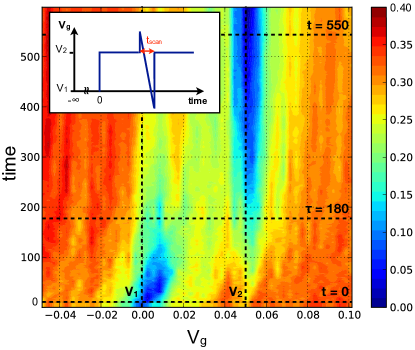
Figure 1: (color online) Normalized time evolution of the DOS as a function of $V_{g}$. Cooler colors represent a lower DOS. Following the protocol shown in the inset: before $t=0$, the Coulomb gap is centred around $V_{1}=0$, at $t=0$ $V_{g}$ is switched to $V_{2}=0.05$ and the original gap slowly disappears, while the new gap around $V_{2}=0.05$ slowly forms. At time $\tau\sim 180$ the two dips have approximately the same depth. Conductance scans in Fig. 2 represent times marked here with dashed lines. The slight swerve of the fading dip may be due to an effect of the leads.

While Fig. 1 describes the DOS, experimentally one measure the conductance between the leads. We calculate the latter using two methods: the first tentative evaluation follows Mott’s relation Mott (1969) between conductance, temperature and the DOS, through the following relation:

$$G(\mu,T)\propto e^{-\left(\frac{T_{0}(\mu)}{T}\right)^{\frac{1}{d+1}}}=e^{-\left(\frac{1}{g(\mu)\xi^{d}T}\right)^{\frac{1}{d+1}}},$$ (5)

where $g(\mu)$ is the DOS at the Fermi level. We can emulate the voltage scans carried out in the TDE by noting that $V_{g}$ sets the Fermi level of the system, and by assuming that within a small enough energy band the DOS can be considered constant. We can then calculate $\sigma(V_{g})$, different $V_{g}$ represented by different $\mu$ (Fermi levels) as mentioned above, and substituting the appropriate value of the calculated DOS in Eq. (5) .

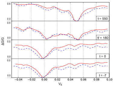
Figure 2: (color online) A successful reproduction of the TDE scans $G(V_{g})$ at different times, using two methods: solid lines use Mott’s relation, Eq. (5), and dashed lines use the Miller-Abrahams random resistor approach, Eq. (6). The scans are calculated for times marked in Fig. 1: (a) $t=-7$, at equilibrium with $V_{1}=0$, (b) $t=1$, $V_{g}$ is changed to $V_{2}=0.05$, (c) $\tau=180$, the time at which the two dips are of the same depth, (d) $t=550$, the new dip at $V_{2}=0.05$ has formed completely.

A systematic evaluation of the conductance uses the Miller-Abrahams random resistor network approach Shklovskii and Efros (1984), i.e the current between donors $i$ and $j$ is expressed through the transmission rates: $J_{ij}=-e(\Gamma_{ij}-\Gamma_{ji})$. We divide the total current by the voltage between the leads, chosen to be $\Delta V=2\times 10^{-5}$. The total conductance is the sum of the conductances between each site and the lead with the lower potential:

$$G(V_{g})=-\frac{e}{\Delta V}\sum_{i}{\left(\Gamma_{iR}(V_{g})-\Gamma_{Ri}(V_{g})\right)}.$$ (6)

We thus emulate again the contuctance scans by calculating the conductance in Eq. (6) for different $V_{g}$ (raising or lowering the energy of the system appropriately). The conductance scans calculated in both methods, for the same four times as marked by dashed lines in Fig. 1, are shown in Fig. 2. It turns out that the two methods agree, successfully reproducing the TDE results. The data was smoothed by averaging over every three consecutive data points. Owing to the lack of a prefactor in Eq. (5), the conductances had to be scaled by a multiplication factor to allow a comparison.

We further verify our results by ascertaining that the relaxation process is logarithmic, namely that the conductance at $V_{1}$ ($V_{2}$), i.e., the bottom of the initial dip (new dip) increases (decreases) logarithmically. This is shown in Fig. 3, where apart from the expected logarithmic relaxation, one can appreciate the explicit coexistence of the two dips.

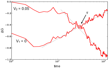
Figure 3: The logarithmic relaxation of the two dips, and their explicit co-existence. We plot the minima of the conductance dips relative to $G_{n}$, the conductance far from the dip ($\Delta G=G-G_{n}$), as a function of time. The curve marked $V_{1}=0$ is the slowly increasing conductance at the original dip, and the curve marked $V_{2}=0.05$ represents the slowly decreasing conductance at the new forming dip. The time axis is in log scale. Dotted lines are guides for the eye. The intersection of the lines yields $\tau$, the time at which the two dips have equal depths.

We now proceed to examine the dependence of $\tau$ and the width of the dip $\Gamma$ on various physical parameters. From Eq. (1) we expect $\Gamma$ to be wider for stronger interactions, as also verified experimentally Vaknin et al. (1998). Our model correctly reproduces this result, shown in Fig. 4. Secondly, from the transition rates in Eq. (3) we expect $\tau$ to decrease as one increases the localization length $\xi$. This behavior is indeed recovered by our model, and is given in the inset of Fig. 4.

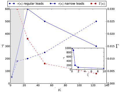
Figure 4: (color online) The width of the dip $\Gamma$ taken from the DOS, (squares, scale on right) vs. the permittivity $\kappa$, which sets the scale of the interaction strength. We find the expected trend of stronger interactions leading to a wider dip, as in Eq. (1). Qualitative analysis of $\tau$ (circles, scale at left) vs. $\kappa$: the dashed line represents a square system ($5\times 5$ in units of $r_{nn}$) and the solid line represents a system with relatively short leads (a $2\times 12.5$ system). Large leads result in a dominant domino effect, where strong interactions lead to faster relaxation, as opposed to what is expected in a macroscopic glass. With smaller leads the domino effect is less dominant, revealing the expected opposite trend of the relaxation process. The greyed area marks strong interactions of the same scale as the energy disorder (i.e., $e^{2}/(\kappa r_{nn})\gtrapprox W$) , where the domino effect is dominant even with smaller leads. Inset: $\tau$ as a function of localization length $\xi$, showing the expected trend: $\tau$ decreases with $\xi$.

Next let us consider the effect of interaction strength on the relaxation process: in glassy systems the relaxation of the system is expected to become slower with stronger interactions, or smaller permittivity $\kappa$. As shown in Fig. 4, the opposite trend is found. This unexpected behaviour can be understood when taking into account the fact that system relaxes through its connection to the leads, and may therefore be affected by them. Indeed upon raising (lowering) $V_{g}$, one raises (lowers) the energy of the sites in the system, raising (lowering) the initial Fermi energy compared to the potential of the leads. For simplicity we will discuss the first case of raising $V_{g}$, but the argument for lowering $V_{g}$ is similar. When the Fermi level is raised the electrons with excess energy compared to the potential of the leads leave the system, and the system reorders and relaxes to its new configuration. We find that when an electron leaves the system through one of the leads, it causes a domino effect, i.e it leads to a cascade of electron relaxation behind it, thus speeding up the relaxation in general. The effect is explained in Fig. 5.

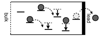
Figure 5: A schematic representation of the finite size domino effect caused by the leads on the system. On the right is the connection to one of the leads. An electron leaves the system through the lead, lowering the energy of other sites by the Coulomb energy that is lost, $\frac{e^{2}}{\kappa r_{ij}}$. Electrons farther from the lead will now hop to the sites with newly lowered energy. This progressive process of lowering the energy of the sites can dramatically speed up the relaxation process, washing out the excess electrons through the leads, stronger interactions leading to faster relaxations, as opposed to what is expected in glassy systems.

To verify that this reversal is indeed due to the leads, we minimized the the effect of the leads by changing the aspect ratio of the system so as to diminish the relative size of the leads. Originally we used a square system $5\times 5$ (in units of $r_{nn}$), and we now used a system $2\times 12.5$, where the leads are of width $2$, and the area, i.e. the size of the system, is left the same. In this case we indeed find that relaxation times in general are longer, and the expected dependence of $\tau$ on the interaction is recovered. For very strong interactions, of the order of the energy disorder (i.e., $e^{2}/(\kappa r_{nn})\approx W$), the domino effect becomes dominant again in spite of the relatively small leads. The results for the square system and the one with narrow leads are compared in Fig. 4. We point out that this effect may also account for the slight swerve of the original dip to lower energies visible in Fig. 1; in this approach electrons with higher energy tend to leave the system more quickly , effectively lowering the original Fermi level. Indeed we noted that for weaker interactions the swerve is less evident. This issue deserves further investigation.

We note that our model differs from real systems in a few aspects: the systems studied experimentally include amorphous and granular metals, where electrons are thought to tunnel between puddles of electrons rather than single occupancy sites (as in our model), and more so it is also expected that simultaneous many-electron transitions may take place Baranovskii et al. (1979) (disregarded in our model). Secondly, in the experiments on amorphous materials one controls the physical paramters such as $\xi$ and $\kappa$ indirectly through the carrier density. The dependence of $\kappa$ and $\xi$ on $n$ is not universal and may depends on details of the system (such as distance to screening gates) that are not fully understood.

The electron glass exhibits interesting memory effects due to ergodicity breaking and aging, which are manifested in the TDE protocol in the form of complex dynamics of the occupation numbers and DOS. In this work we successfully reproduced numerically these experimental results for the first time, by describing the evolution of the average occupation numbers of sites using kinetic equations, in a local mean-field approach. Due to the far-from-equilibrium nature of the problem, we could not use the linear approximation as done before, and were compelled to solve the full nonlinear coupled equations. The verification of the logarithmic relaxation of the dip together with our understanding of the dependence of $\tau$ and $\Gamma$ on the main physical parameters of the system, $\xi$ and $\kappa$, leaves us with a complete characterization of our model, which successfully captures the TDE behavior. Moreover we unveiled an important finite size domino effect on the relaxation process caused by the leads in the experimental setup, which not only speeds up the relaxation process in general, but can also reverse the dependence of the relaxation process on the interaction strength. This effect should be taken into consideration when dealing with mesoscopic systems or ones with strong interactions.

Aknowledgments We would like to thank Ariel Amir, Thierry Grenet, Markus Müller and Zvi Ovadyahu for fruitful discussions. This work was supported by the German-Israeli Foundation (GIF).

References

- Ben-Chorin et al. (1991) M. Ben-Chorin, D. Kowal, and Z. Ovadyahu, Phys. Rev. B 44, 3420 (1991).
- Ben-Chorin et al. (1993) M. Ben-Chorin, Z. Ovadyahu, and M. Pollak, Phys. Rev. B 48, 15025 (1993).
- Ovadyahu (2008) Z. Ovadyahu, Phys. Rev. B 78, 195120 (2008).
- Ovadyahu and Pollak (1997) Z. Ovadyahu and M. Pollak, Phys. Rev. Lett. 79, 459 (1997).
- Vaknin et al. (1998) A. Vaknin, Z. Ovadyahu, and M. Pollak, Phys. Rev. Lett. 81, 669 (1998).
- Ovadyahu (2007) Z. Ovadyahu, Physical Review Letters 99, 226603 (2007).
- Grenet et al. (2007) T. Grenet, J. Delahaye, M. Sabra, and F. Gay, The European Physical Journal B 56, 183 (2007).
- Grenet and Delahaye (2010) T. Grenet and J. Delahaye, The European Physical Journal B 76, 229 (2010).
- Grenet and Delahaye (2012) T. Grenet and J. Delahaye, Phys. Rev. B 85, 235114 (2012).
- Orlyanchik and Ovadyahu (2004) V. Orlyanchik and Z. Ovadyahu, Physical Review Letters 92, 066801 (2004).
- Thouless et al. (1977) D. Thouless, P. Anderson, and R. Palmer, Philos. Mag. 35, 593 (1977).
- Grunewald et al. (1982) M. Grunewald, B. Pohlmann, L. Schweitzer, and D. Wurtz, J. Phys. C 15, L1153 (1982).
- Amir et al. (2011) A. Amir, Y. Oreg, and Y. Imry, Annu. Rev. Condens. Matter Phys. 2, 235 (2011).
- Pollak (1970) M. Pollak, Discuss. Faraday Soc. 50, 13 (1970).
- Efros and Shklovskii (1975) A. L. Efros and B. I. Shklovskii, J. Phys. C 8, L49 (1975).
- Efros (1976) A. L. Efros, J. Phys. C 9, 2021 (1976).
- Monroe et al. (1987) D. Monroe, A. Gossard, J. English, B. Golding, W. Haemmerle, and M. Kastner, Physical Review Letters 59, 1148 (1987).
- Amir et al. (2008) A. Amir, Y. Oreg, and Y. Imry, Phys. Rev. B 77, 165207 (2008).
- Amir et al. (2009a) A. Amir, Y. Oreg, and Y. Imry, Phys. Rev. Lett. 103, 126403 (2009a).
- Amir et al. (2009b) A. Amir, Y. Oreg, and Y. Imry, Phys. Rev. B 80, 245214 (2009b).
- Mott (1969) N. F. Mott, Philos. Mag. 19, 835 (1969).
- Shklovskii and Efros (1984) B. Shklovskii and A. Efros, Electronic properties of doped semiconductors (Berlin: Springer-Verlag, 1984).
- Baranovskii et al. (1979) S. Baranovskii, A. Efros, B. Gelmont, and B. Shklovskii, Journal of Physics C: Solid State Physics 12, 1023 (1979).
- Lebanon and Müller (2005) E. Lebanon and M. Müller, Physical Review B 72, 174202 (2005).
- Levin et al. (1987) E. Levin, V. Nguyen, B. Shklovskii, and A. Efros, Sov. Phys. JETP 65, 842 (1987).
- Mogilyanskii and Raikh (1989) A. Mogilyanskii and M. Raikh, Sov. Phys. JETP 68, 1081 (1989).