“DIRECT” GAS-PHASE METALLICITIES, STELLAR PROPERTIES, AND LOCAL ENVIRONMENTS OF EMISSION-LINE GALAXIES AT REDSHIFTS BELOW 0.90

Abstract

Using deep narrow-band (NB) imaging and optical spectroscopy from the Keck telescope and MMT, we identify a sample of 20 emission-line galaxies (ELGs) at $z=0.065$–0.90 where the weak auroral emission line, [O iii] $\lambda$4363, is detected at $\geq$3$\sigma$. These detections allow us to determine the gas-phase metallicity using the “direct” method. With electron temperature measurements, and dust attenuation corrections from Balmer decrements, we find that 4 of these low-mass galaxies are extremely metal-poor with 12 + $\log({\rm O/H})$ $\leq$ 7.65 or one-tenth solar. Our most metal-deficient galaxy has 12 + $\log({\rm O/H})$= 7.24${}^{+0.45}_{-0.30}$ (95% confidence), similar to some of the lowest metallicity galaxies identified in the local universe. We find that our galaxies are all undergoing significant star formation with average specific star formation rate (SFR) of (100 Myr)^-1, and that they have high central SFR surface densities (average of 0.5 $M_{\sun}$ yr^-1 kpc^-2). In addition, more than two-thirds of our galaxies have between one and four nearby companions within a projected radius of 100 kpc, which we find is an excess among star-forming galaxies at $z=$0.4–0.85. We also find that the gas-phase metallicities for a given stellar mass and SFR lie systematically lower than the local $M_{\star}$–$Z$–(SFR) relation by $\approx$0.2 dex (2$\sigma$ significance). These results are partly due to selection effects, since galaxies with strong star formation and low metallicity are more likely to yield [O iii] $\lambda$4363 detections. Finally, the observed higher ionization parameter and high electron density suggest that they are lower redshift analogs to typical $z\gtrsim 1$ galaxies.

1. INTRODUCTION

The chemical enrichment of galaxies, driven by star formation and regulated by gas outflows from supernovae and inflows from cosmic accretion, is a key process in galaxy formation that remains to be fully understood. The greatest difficulty in measuring chemical evolution across all galaxy populations is the need for rest-frame optical spectroscopy. Metallicity determinations can be obtained through (1) interstellar absorption lines (e.g., Fe II, Mg II), and (2) nebular emission lines (e.g., [O ii], [O iii], and [N ii]). While studies have used absorption lines to measure heavy-element abundances (Savaglio et al., 2004), the need for deep spectroscopy and complications with curve-of-growth analysis have made it difficult. As such, the primary method used to measure the metal abundances in galaxies has been nebular emission lines. This technique has the advantage of being able to probe low-luminosity galaxies since it does not require continuum detection. In addition, these emission lines can be observed in the optical and near-infrared (near-IR) at redshifts of $\sim$3 and below with current ground (see e.g., Hayashi et al., 2009; Moustakas et al., 2011; Henry et al., 2013; Momcheva et al., 2013) and space-based capabilities (see e.g., Atek et al., 2010; Xia et al., 2012), and the forthcoming IR capabilities of the James Webb Space Telescope (JWST) will extend this further to $z\approx 6$.

The most reliable metallicity determination is made possible by measuring the flux ratio of the [O iii] $\lambda$4363 auroral line against a lower excitation line, such as [O iii] $\lambda$5007. The technique is often called the $T_{e}$ or “direct” method for its ability to determine the electron temperature ($T_{e}$) of the ionized gas, and hence the gas-phase metallicity (see e.g., Aller, 1984). However, the detection of [O iii] $\lambda$4363 is difficult, as it is very weak (and almost undetectable in metal-rich galaxies). For example, the first data release (DR1) of the Sloan Digital Sky Survey (SDSS; York et al., 2000) only revealed 8 new extremely metal-poor galaxies (XMPGs; 12 + $\log({\rm O/H})$ $\leq 7.65$) among 250,000 galaxies (Kniazev et al., 2003). Even with improved selection and a larger sample ($\approx$530,000), Izotov et al. (2006a) only detected [O iii] $\lambda$4363 at $\geq$2$\sigma$ significance in 310 galaxies (i.e., one in 1700). While SDSS spectra can be stacked for average measurements of [O iii] $\lambda$4363 (Andrews & Martini, 2013, hereafter AM13), this sacrifices knowledge of the intrinsic scatter in the mass-metallicity ($M_{\star}$–$Z$) relation (MZR), which can also constrain galaxy evolution models (see e.g., Davé et al., 2011).

While it is unfortunate that the $T_{e}$ method cannot be used for the full dynamic range of metallicity, the detection in a galaxy of [O iii] $\lambda$4363 alone is a strong indication that it is extremely metal deficient. These rare XMPGs are suspected to be primeval galaxies that are undergoing rapid assembly at the observed redshift (Kniazev et al., 2003, and references therein). Studying larger samples of them can provide a better understanding of the early stages of galaxy assembly.

One possibility is that XMPGs have significant outflows that are induced by supernova from massive star formation. These outflows could drive large amounts of metal-rich gas out of the galaxy, thus decreasing the metal abundances. Studies have found that outflows are prevalent in metal-poor galaxies through (1) detection of outflowing ionized gas from integral field unit (IFU) spectroscopy of an XMPG (Izotov et al., 2006b); (2) blue-shifted absorption lines from slit spectroscopy of star-forming galaxies, suggesting that outflows are ubiquitous (e.g., Weiner et al., 2009; Martin et al., 2012); and (3) evidence that galaxies with higher specific SFR (SFR per unit stellar mass; sSFR $\equiv$ SFR/$M_{\star}$) are more metal poor (Ellison et al., 2008; Lara-López et al., 2010; Mannucci et al., 2010).

Another explanation is that metal-deficient gas is supplied either from the circumgalactic medium (CGM) perhaps through a “cold-mode” accretion phase (Kereš et al., 2005; Dekel et al., 2009) or from the strong interaction with a nearby merging companion (see e.g., Kewley et al., 2006; Rupke et al., 2010).

The two most metal-deficient galaxies known to date are I Zw 18 (Searle & Sargent, 1972) and SBS0335-052 (hereafter, SBS0335; Izotov et al., 1990) with oxygen abundances of 12 + $\log({\rm O/H})$ = 7.14 ($Z_{\sun}$/35; Izotov et al., 2006a) and 7.19–7.34 ($Z_{\sun}$/(23–32); Izotov et al., 1999), respectively. Efforts have been made to increase the galaxy sample with direct metallicity determinations in the local universe (Brown et al., 2008; Berg et al., 2012; Izotov et al., 2012a), and at higher redshift (Hoyos et al., 2005; Kakazu et al., 2007; Hu et al., 2009; Atek et al., 2011). These studies have either targeted galaxies with low luminosity or high equivalent width (EW) emission lines. The latter are found using NB imaging, grism spectroscopy, or unusual broad-band colors to select them. For example, Kakazu et al. (2007) and Hu et al. (2009) utilized NB imaging to select ELGs at $z\sim 0.40$–0.85 and conducted optical follow-up spectroscopy with Keck to detect [O iii] $\lambda$4363 and determine direct metallicity for 28 galaxies. They found one galaxy where their measured metallicity is 12 + $\log({\rm O/H})$ = $6.97\pm 0.17$. To date, only $\approx$70 galaxies are known to have 12 + $\log({\rm O/H})$ $\leq 7.65$ with the majority (90%) of them at $z\lesssim 0.1$.

In this paper, we focus on our spectroscopic detections of [O iii] $\lambda$4363 in 20 galaxies at $z=0.065$–0.90 (average of $z=0.54\pm 0.22$) in the Subaru Deep Field (SDF; Kashikawa et al., 2004). These galaxies were initially selected for their excess flux in NB and/or intermediate-band filters produced by emission lines. In particular, we have rest-frame spectral coverage of at least 3700–5010Å, enabling metallicity determinations using the $T_{e}$ method.

The outline of the paper is as follows. In Section 2 we describe the imaging survey for the SDF, the selection of over 9,000 ELGs, the follow-up optical spectroscopy that we conducted, and our accurate flux calibration approach. We then discuss in Section 3 our approach for detecting and measuring nebular emission lines, which yields a spectroscopic sample with [O iii] $\lambda$4363 detections that are significant at $\geq$3$\sigma$. We also present arguments for why all but one of our galaxies is ionized primarily by young stars. Section 4 then describes how we determine: (1) the dust attenuation properties in our galaxies; (2) the electron temperature and the gas-phase oxygen metallicity; (3) the dust-corrected SFRs; (4) the stellar properties from spectral energy distribution (SED) fitting; (5) the nearby environment; and (6) the SFR surface density. In Section 5, we compare our results to other galaxies that have direct metallicity determinations, and discuss selection effects for our sample. Finally, we estimate the space densities of compact, extreme star-forming, metal-poor galaxies found in this survey, and consider their implications for the broader context of galaxy evolution.

Throughout this paper, we adopt a flat cosmology with $\Omega_{\Lambda}=0.7$, $\Omega_{M}=0.3$, and $H_{0}=70$ km s^-1 Mpc^-1 to determine distance-dependent measurements, and magnitudes are reported on the AB system (Oke, 1974). For reference, we adopt 12 + $\log({\rm O/H})$_☉ = 8.69 (Allende Prieto et al., 2001) for metallicity measurements quoted against the solar value, $Z_{\sun}$. Unless otherwise indicated, we report 95% confidence measurement uncertainties, and “[O iii]” alone refers to the strong 5007Å emission line.

2. THE SUBARU DEEP FIELD

The SDF has the most sensitive optical imaging in several NB and intermediate (IA) filters in the sky, and is further complemented with ultra-deep multi-band imaging between 1500Å and 4.5$\mu$m. A summary of the ancillary imaging is available in Ly et al. (2011a) and later in Section 4.4. The results for this paper are based on data obtained in the NB704, NB711, NB816, NB921, NB973, IA598, and IA679 filters. A summary of their properties (i.e., central wavelength, sensitivity) is reported in Table 1, and Figure 1 shows the total system response through these filters and the surveyed redshifts.

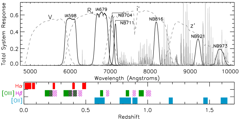
Figure 1.— Top: Total system throughput for the $VR_{\rm C}i\arcmin z\arcmin$ filters (gray dashed lines) and the IA598, IA679, NB704, NB711, NB816, NB921, and NB973 filters (black solid lines). Bottom: Redshift ranges probed when H$\alpha$, [O iii], H$\beta$, and [O ii] are redshifted into these filters. The SDF probes 64% of redshift space and 67% of comoving volume at $z\leq 1.03$.

Table 1Summary of Filters, Emission-line Samples, and Redshift Windows

Filter	$\lambda_{c}$	FWHM	$m_{\rm lim}(3\sigma)$	Area	$N_{\rm total}$	$N_{\rm target}$	$N_{\rm spec}$	$z$(H$\alpha$)	$z$([O iii])	$z$([O ii])
	[Å]	[Å]	[mag]	[arcmin2]
(1)	(2)	(3)	(4)	(5)	(6)	(7)	(8)	(9)	(10)	(11)
IA598	6007	303	26.79	870.4	641	string31	string21	…	0.170–0.230	0.571–0.652
IA679	6780	340	27.39	870.4	790	string76	string54	0.007–0.059	0.320–0.388	0.774–0.865
NB704	7046	100	26.71	870.4	1695	173	140	0.066–0.081	0.397–0.417	0.877–0.904
NB711	7111	string72	26.07	870.4	1480	111	string92	0.078–0.089	0.413–0.427	0.898–0.918
NB816	8150	120	26.90	870.4	1602	300	204	0.233–0.251	0.616–0.640	1.171–1.203
NB921	9196	132	26.71	870.4	2361	251	185	0.391–0.411	0.824–0.850	1.450–1.485
NB973	9755	200	25.69	788.7	1243	string71	string63	0.471–0.502	0.928–0.968	1.591–1.644
Total	…	…	…	…	9264	870	713	…	…	…

Note. — We report the numbers of excess emitters ($N_{\rm total}$) in Col. (6), the numbers of galaxies with targeted MMT and/or Keck spectra ($N_{\rm target}$) in Col. (7), and the sub-sample with robust spectroscopic redshift ($N_{\rm spec}$) in Col. (8).

These SDF data were acquired with Suprime-Cam (Miyazaki et al., 2002), the optical imager mounted at the prime focus of the Subaru telescope, between 2001 March and 2007 May. The acquisition and reduction of these data have been discussed extensively in Kashikawa et al. (2004), Kashikawa et al. (2006), Ly et al. (2007) (hereafter L07), and Ly et al. (2012b) for the NB data, and in Nagao et al. (2008) for the IA data. In brief, data were obtained mostly in photometric conditions with average seeing of 0$\farcs$9–1$\farcs$0 for all five NB and two IA filters. These data were reduced following standard reduction procedures using sdfred (Yagi et al., 2002; Ouchi et al., 2004), a software package designed especially for Suprime-Cam data.

The most prominent emission lines entering these NB and IA filters are H$\alpha$, [O iii], H$\beta$, and [O ii], at well-defined redshift windows between $z=0.01$ and $z=1.62$. This results in probing 64% in redshift space and 67% of the available comoving volume at $z\leq 1.03$. Compared to the previous NB survey for XMPGs at $z=0.24$–0.85 (Hu et al., 2009), our survey probes 4.7 (3.8) times more redshift (volume) space, and is deeper by $\approx$1.5 mag in the NB filters.

2.1. Selection of Emission-line Galaxies

To select NB and IA excess emitters due to the presence of nebular emission line(s), we use the standard color excess selection, where photometric fluxes from these filters are compared against those for adjacent broad-band filters that sample the continuum. Since the technique has been extensively used, we briefly summarize it below, referring readers to Fujita et al. (2003) and Ly et al. (2011b). We summarize our excess emitter sample in Table 1.

The measured continuum adjacent to the line is determined by the two broad-band filters closest to the narrow bandpass. For NB921 and NB973, we start with the $z$′-band. Since the central wavelengths of these filters are redder than what the $z$′ filter measures, we correct for such differences using the $i$′–$z$′ color (Ly et al., 2012a, b). The remaining filters use a flux-weighted combination of either the $V$- and $R_{\rm C}$-band (IA598), the $R_{\rm C}$- and $i$′-band (NB704, NB711, and IA679), or the $i$′- and $z$′-band (NB816):

$$f_{\rm cont}=\epsilon f_{\rm blue}+(1-\epsilon)f_{\rm red},$$ (1)

where $f_{\rm blue}$ and $f_{\rm red}$ are the flux density in erg s^-1 cm^-2 Hz^-1 for the bluer and redder broad-band filters, respectively (e.g., $i$′ and $z$′ for NB816), and $\epsilon=$ 0.45 (IA598), 0.5 (NB704, NB711), 0.75 (IA679), and 0.6 (NB816).

Photometric measurements for broad-band data are obtained by running SExtractor (Bertin & Arnouts, 1996) in “dual-image” mode, where the respective NB or IA image is used as the “detection” image. This works well because all broad-band, IA, and NB mosaicked images have very similar seeing, so that excess colors are determined within the same physical scale of the galaxies. For the extraction of fluxes and selection of sources, we use a 2″ diameter circular aperture. For comparison, the 3$\sigma$ sensitivities for the $V$, $R_{\rm C}$, $i$′, and $z$′ data are between 26.27 and 27.53 mag, which are generally deeper than the NB and IA imaging.

We also exclude sources which fall in regions affected by poor coverage and contamination by bright foreground stars. The unmasked regions cover 870.4 arcmin² for all filters with the exception of NB973, which covers 788.7 arcmin². The latter is smaller due to higher systematic noise in one of the ten CCDs, which we mask to avoid significant spurious detections. In total, 123123, 97632, 133273, 119541, 84786, 118097, and 139585 sources are detected in the unmasked regions of the NB704, NB711, NB816, NB921, NB973, IA598, and IA679 mosaics, respectively. Among these sources, 1695, 1480, 1602, 2361, 1243, 641, and 790 are identified as NB or IA excess emitters.

In certain circumstances, our sources are selected by more than one filter. This is due to some fortuitous redshift overlap of our NB/IA filters such that different emission lines (e.g., H$\alpha$ and [O iii]) are detectable at the same redshift (see Figure 1). Accounting for duplicate galaxies, the complete SDF ELG sample consists of 9264 galaxies mostly at $z=0.01$ to $z=1.62$ with some at higher redshift due to Ly$\alpha$ emission. We note that the sample presented in this paper supersedes our earlier multi-NB studies. Previously, we had selected ELGs in four NB filters and examined the evolution of the H$\alpha$, [O iii], and [O ii] luminosity functions (L07). A fifth NB filter (NB973) was later included, and that filter allowed us to study dust attenuation at $z=0.4$–0.5 (Ly et al., 2012a) and stellar properties out to $z=1.5$–1.6 (Ly et al., 2012b).

2.2. Optical Spectroscopy

The primary results of this paper are based on optical spectroscopy taken over the past several years, with Keck’s Deep Imaging Multi-Object Spectrograph (DEIMOS; Faber et al., 2003) and MMT’s Hectospec (Fabricant et al., 2005). In total, we obtained 945 optical spectra for 870 ELGs, and successfully detected emission lines to determine redshift for 713 galaxies or 82% of the targeted sample. These spectra were initially obtained to confirm that the NB technique efficiently identified ELGs. A summary of the spectroscopically confirmed excess emitters is provided in Table 1.

The majority (61%) of our spectroscopic sample was obtained from Hectospec. These spectra were obtained between 2008 Mar 13 and 2008 Apr 14, utilizing the 270 mm^-1 grating blazed at 5200Å to yield spectral coverage of 3650Å–9200Å. The combination of this grating with a fiber diameter of 1$\farcs$5 yields a spectral resolution of $\approx$6Å.

The typical seeing for these observations was between 0$\farcs$7 and 1$\farcs$4, and the data were obtained at airmasses below 1.35, with 95% (77%) of the data below 1.3 (1.2). Four different fiber configurations were used, with on-source integrations varying between 4 and 6 20-min exposures, which is sufficient for cosmic ray rejection. The MMT spectra were reduced following standard procedures with the iraf Hectospec Reduction Software. Since no order-blocking filter was used, the spectra at wavelengths longward of 8200Å have a significant amount of contaminating second-order light (up to 30% for the relatively blue flux standard stars). The flux calibration in the far-red is therefore unreliable, and we do not use it.

The Keck/DEIMOS observations were obtained in 2004, 2008, and 2009. The 2004 spectroscopic observations have been discussed in Kashikawa et al. (2006) and L07, and the more recent data have been discussed in Kashikawa et al. (2011). In brief, we constructed 13 slit-masks with 1″ slit widths. This typically corresponds to a spectral resolution of $R\sim 3600$ at 8500Å, and spectral dispersion of 0.47Å pixel^-1. The 830 line mm^-1 grating and GG495 order-cut filter were used in all DEIMOS observations. This set-up resulted in a spectral coverage of $\approx$5000Å–1$\mu$m; however the coverage varied along the dispersion axis of the slit mask. The typical seeing for these observations was 0$\farcs$5–1$\farcs$0 in 2004 and 0$\farcs$7-1$\farcs$1 for 2008–2009 with integration times of 2–3 hr. Almost all (86%) of the DEIMOS spectra were obtained at low airmasses ($\leq$1.3), with the remaining data taken at an airmass of 1.35.

2.2.1 Flux Calibration

The metallicities that we will determine require measurements between 3700Å and 5010Å in the rest-frame, thus accurate flux calibration is critical. We follow a rigorous approach: we (1) observe spectro-photometric standards to account for the wavelength-dependent sensitivity of each spectrograph; (2) correct for slit losses by comparing spectra against broad-band photometric data; (3) compare emission-line fluxes against NB photometry to assess the accuracy of flux calibration; and (4) compare spectra obtained on different nights for a few dozen multiply-observed galaxies. A more detailed description of the flux calibration for our MMT/Hectospec and Keck/DEIMOS spectra is deferred to Appendix A. In brief, our various independent tests and analyses yielded consistent results, and demonstrated that the absolute flux calibration is reliable at the 0.15–0.17 dex (0.12–0.17 dex) level for Hectospec (DEIMOS).

3. THE [O iii] $\lambda$4363 SAMPLE

To extract fluxes for strong and weak emission lines in these spectra, we fit each line with a Gaussian profile using the IDL routine mpfit (Markwardt, 2009). The expected location of emission lines was based on a priori redshift determined by either the [O iii] or H$\alpha$ (for lower redshift). A local median, $\left<f\right>$, is computed within a 200Å-wide region, excluding regions affected by OH skylines and nebular emissions. In addition, the standard deviation $\sigma(f)$ is measured locally. Examples of the computed medians and standard deviations are shown in Figure 2. To determine the significance of emission lines, we integrate the spectrum between $l_{C}-2.5\sigma_{G}$ and $l_{C}+2.5\sigma_{G}$, where $\sigma_{G}$ is the Gaussian width:

$${\rm Flux}\equiv\sum_{-2.5\sigma_{G}}^{+2.5\sigma_{G}}\left[f(\lambda-l_{C})-\left<f\right>\right]\times l\arcmin.$$ (2)

Here, $l$′ is the spectral dispersion (1.21Å pixel^-1 for MMT and $\approx$0.47Å pixel^-1 for Keck). We then compute the signal-to-noise (S/N) of the line by dividing the integrated flux by:

$${\rm Noise}\equiv\sigma(f)\times l\arcmin\times\sqrt{N_{\rm pixel}},$$ (3)

where $N_{\rm pixel}=5\sigma_{G}/l$′.

Adopting a minimum significance threshold of 3$\sigma$, we identify 20 and 14 [O iii] $\lambda$4363 detections with MMT and Keck, respectively. We visually inspected each [O iii] $\lambda$4363 detection. For MMT, we found that OH sky-lines contaminated [O iii] $\lambda$4363 in three cases, and H$\beta$ in three other galaxies. This results in a final sample of 14 [O iii] $\lambda$4363 detections. For Keck, OH sky-lines contaminated [O iii] $\lambda$4363 in three cases and [O ii] measurements in two other cases, while three sources lack full spectral coverage (missing [O ii], H$\beta$, and/or [O iii] $\lambda\lambda$4959,5007). This reduced the [O iii] $\lambda$4363 Keck sample to 6 galaxies.

Our final sample of [O iii] $\lambda$4363 detections, hereafter the “[O iii]-A” sample, consists of 20 galaxies. The MMT and Keck [O iii] $\lambda$4363 detections are shown in Figure 2 with the full MMT (Keck) spectra provided in Figures 14–15 (Figure 16). We also summarize our [O iii] $\lambda$4363 sample in Table 2. For convenience, our galaxies are identified as “MMT” and “Keck” followed by a sequential number. In Table 3, we provide the [O ii], H$\beta$, and [O iii] emission-line fluxes along with the $O_{32}$ and $R_{23}$ (Pagel et al., 1979) flux ratios:

$$O_{32} \equiv \frac{[{\rm O}~{}\textsc{iii}]\,\lambda\lambda 4959,5007}{[{\rm O}~{}\textsc{ii}]\,\lambda\lambda 3726,3729},{\rm~{}and}$$ (4)

$$R_{23} \equiv \frac{[{\rm O}~{}\textsc{ii}]\,\lambda\lambda 3726,3729+[{\rm O}~{}\textsc{iii}]\,\lambda\lambda 4959,5007}{{\rm H}\beta}.$$ (5)

Also, emission-line luminosities and rest-frame EWs (EW₀) are illustrated in Figure 3. The latter are determined by measuring the continuum from the SEDs with corrections for emission-line contamination (see Section 4.4). The former is $L=4\pi d_{L}^{2}F_{\rm Line}$, where $d_{L}$ is the luminosity distance, and $F_{\rm Line}$ is the emission-line flux.

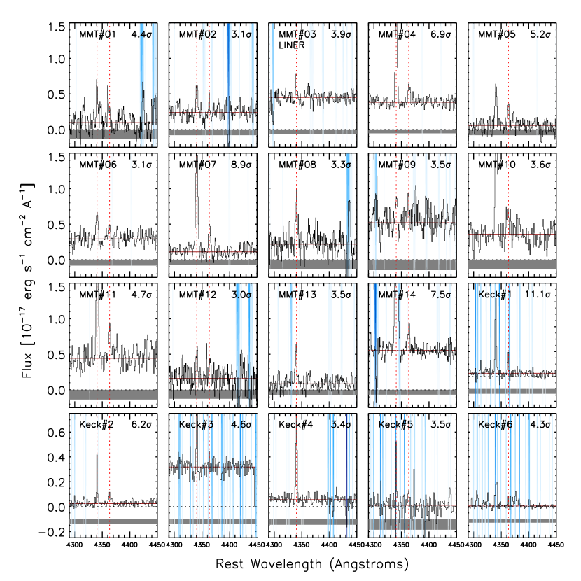
Figure 2.— Detections of [O iii] $\lambda$4363 in 20 galaxies. The rest-frame spectra are shown in black, with vertical red dashed lines indicating the locations of H$\gamma$ $\lambda$4340 and [O iii] $\lambda$4363. OH sky-lines are indicated by blue vertical bands, where the strength of the sky-lines is denoted by their shade of blue (darker is stronger). The grey-shaded regions indicate the locally measured 1$\sigma$ noise, while the horizontal brown lines correspond to the median of the continua.

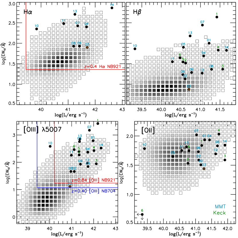
Figure 3.— Emission-line luminosities and rest-frame EWs for our [O iii]-A sample. All fluxes are observed, before correction for dust attenuation. Gray squares illustrate the SDSS DR7 emission-line sample with at least 5$\sigma$ detections in all four lines. The density of sources is shown with a linear scale from white (low) to black (highest). Our only LINER (MMT#03) is denoted by the orange crosses. For comparative purposes, we show the EW and luminosity limits of our NB921 imaging (solid red lines) for $z=0.4$ H$\alpha$ (top left) and $z=0.84$ [O iii] (bottom left) and NB704 imaging (solid blue lines) for $z=0.4$ [O iii]. The MMT sample is labelled in blue while the Keck sample is indicated in green.

We note that for two galaxies (MMT#04 and MMT#07), spectra were obtained with two different MMT/Hectospec fiber configurations. In both cases, [O iii] $\lambda$4363 was detected in each spectrum, confirming that these detections are robust. For these two galaxies, we combine the spectra for a higher S/N spectrum. In addition, more recent MMT/Hectospec observations for MMT#01, #03–#05, #07, #10, and #13 were taken in less ideal observing conditions. These observations also detected [O iii] $\lambda$4363 in MMT#04, #07, and possibly #13. Since these spectra are less sensitive than those obtained in 2008, we do not combine them for the purpose of our analyses.

Table 2Summary of Spectroscopic Sample

ID	Name	Line Sel.	R.A.	Dec.	$z_{\rm spec}$	Obs. Dates (UT)	$t_{\rm int}$
			[hr]	[deg]			[min.]
(1)	(2)	(3)	(4)	(5)	(6)	(7)	(8)
MMT#01	NB816–140623	[O iii]	13:25:16.87	27:39:06.92	0.6380	2008 Apr 14	120
MMT#02	NB711–064628	[O iii]	13:23:39.13	27:32:52.71	0.4327	2008 Mar 13	120
MMT#03	NB973–104154	H$\alpha$	13:23:39.17	27:31:47.34	0.4809	2008 Mar 13	120
MMT#04	NB704–088982_NB921–126525_IA679–112491	[O iii],H$\alpha$	13:24:46.63	27:34:56.98	0.3933	2008 Mar 13, Apr 11	240
MMT#05	IA679–031637	[O iii]	13:25:03.37	27:17:23.77	0.3846	2008 Mar 13	120
MMT#06	NB704–036405_NB921–063205	[O iii],H$\alpha$	13:23:54.77	27:20:12.53	0.3995	2008 Mar 13	120
MMT#07	NB704–049936_NB921–079428_IA679–062450	[O iii],H$\alpha$	13:24:06.94	27:24:01.76	0.3896	2008 Mar 13, Apr 11	240
MMT#08	NB816–081644	[O iii]	13:23:42.97	27:26:35.59	0.6335	2008 Apr 10	string80
MMT#09	NB973–094500	H$\alpha$	13:23:49.80	27:28:35.32	0.4788	2008 Apr 10	string80
MMT#10	NB704–009999	H$\alpha$	13:23:56.39	27:13:32.98	0.0683	2008 Apr 10	string80
MMT#11	IA598–079010	[O iii]	13:24:13.64	27:25:09.27	0.1752	2008 Apr 10	string80
MMT#12	NB816–112403	[O iii]	13:25:21.78	27:33:15.69	0.6405	2008 Apr 10	string80
MMT#13	NB711–102472_NB973–156739	H$\beta$,H$\alpha$	13:24:28.88	27:45:51.88	0.4696	2008 Apr 11	120
MMT#14	NB711–077774_NB973–125003	H$\beta$,H$\alpha$	13:25:22.94	27:37:40.33	0.4644	2008 Apr 11	120
Keck#1	NB711–049857_IA679–079866_NB921–995851	[O iii]	13:25:11.94	27:27:31.20	0.8390	2004 Apr 23	120
Keck#2	NB816–070113	[O iii]	13:24:34.91	27:24:10.20	0.6230	2004 Apr 23	118
Keck#3	IA679–077341	[O ii]	13:23:53.54	27:27:13.01	0.7906	2004 Apr 23	118
Keck#4	NB704–087569	[O ii]	13:23:43.51	27:34:20.98	0.8829	2008 May 1	130
Keck#5	NB921–078003	[O iii]	13:24:43.66	27:23:34.86	0.8353	2009 Apr 27	180
Keck#6	NB704–060432	[O iii]	13:24:58.62	27:26:40.47	0.8237	2009 Apr 27	180

Table 3Emission-line Measurements and Flux Ratios

ID	[O ii]	H$\beta$	[O iii] $\lambda$4959	[O iii] $\lambda$5007	[O iii] $\lambda$4363	S/N(4363)	$R_{23}$	$O_{32}$
(1)	(2)	(3)	(4)	(5)	(6)	(7)	(8)	(9)
MMT#01	11.05$\pm$0.59	9.55$\pm$0.78string	19.12$\pm$1.04	54.30$\pm$0.70string	2.20$\pm$0.50	4.44	8.85${}^{+1.18}_{-1.12}$	6.64${}^{+0.44}_{-0.41}$
MMT#02	18.55$\pm$0.35	5.93$\pm$0.27string	6.73$\pm$0.27	19.41$\pm$0.28string	0.64$\pm$0.21	3.06	7.54${}^{+0.53}_{-0.41}$	1.41${}^{+0.05}_{-0.05}$
MMT#03	20.94$\pm$0.46	5.79$\pm$0.27string	3.13$\pm$0.39	9.51$\pm$0.31string	0.84$\pm$0.21	3.95	5.80${}^{+0.26}_{-0.34}$	0.60${}^{+0.03}_{-0.03}$
MMT#04	50.23$\pm$0.28	22.17$\pm$0.17string	32.13$\pm$0.26	99.65$\pm$0.24string	1.48$\pm$0.22	6.86	8.21${}^{+0.05}_{-0.06}$	2.62${}^{+0.02}_{-0.02}$
MMT#05	3.84$\pm$0.36	7.09$\pm$0.25string	15.15$\pm$0.24	43.97$\pm$0.26string	1.30$\pm$0.25	5.22	8.88${}^{+0.40}_{-0.32}$	15.38${}^{+1.39}_{-1.68}$
MMT#06	21.76$\pm$0.34	6.31$\pm$0.34string	5.66$\pm$0.29	16.34$\pm$0.26string	0.84$\pm$0.27	3.10	6.94${}^{+0.41}_{-0.41}$	1.01${}^{+0.03}_{-0.02}$
MMT#07	20.15$\pm$0.28	21.06$\pm$0.20string	35.97$\pm$0.24	120.77$\pm$0.24string	2.28$\pm$0.26	8.91	8.40${}^{+0.10}_{-0.10}$	7.78${}^{+0.11}_{-0.08}$
MMT#08	28.23$\pm$0.71	11.21$\pm$1.27string	10.47$\pm$1.04	32.57$\pm$0.89string	1.85$\pm$0.56	3.32	6.36${}^{+0.58}_{-0.64}$	1.52${}^{+0.08}_{-0.09}$
MMT#09	16.88$\pm$0.82	6.81$\pm$0.62string	10.37$\pm$1.12	28.96$\pm$1.17string	1.45$\pm$0.41	3.53	8.26${}^{+0.31}_{-0.71}$	2.33${}^{+0.05}_{-0.10}$
MMT#10	22.70$\pm$1.06	18.55$\pm$0.42string	30.93$\pm$0.45	92.80$\pm$0.52string	2.22$\pm$0.62	3.58	7.89${}^{+0.14}_{-0.21}$	5.45${}^{+0.21}_{-0.25}$
MMT#11	43.34$\pm$0.75	22.30$\pm$0.57string	35.26$\pm$0.60	112.99$\pm$0.63string	2.08$\pm$0.45	4.67	8.59${}^{+0.20}_{-0.24}$	3.42${}^{+0.06}_{-0.07}$
MMT#12	24.18$\pm$0.68	6.30$\pm$0.93string	11.29$\pm$0.77	29.59$\pm$0.73string	1.46$\pm$0.48	3.04	10.32${}^{+1.84}_{-1.82}$	1.69${}^{+0.07}_{-0.07}$
MMT#13	6.33$\pm$0.54	6.55$\pm$0.26string	10.94$\pm$0.39	28.50$\pm$0.45string	1.07$\pm$0.31	3.46	6.99${}^{+0.33}_{-0.34}$	6.23${}^{+0.66}_{-0.63}$
MMT#14	102.13$\pm$0.54	57.20$\pm$0.34string	87.06$\pm$0.61	269.12$\pm$0.67string	2.14$\pm$0.28	7.55	8.01${}^{+0.07}_{-0.06}$	3.49${}^{+0.02}_{-0.02}$
Keck#1	4.61$\pm$0.14	7.72$\pm$0.09string	15.35$\pm$0.09	45.52$\pm$0.08string	0.74$\pm$0.07	11.13	8.49${}^{+0.10}_{-0.09}$	13.21${}^{+0.46}_{-0.45}$
Keck#2	3.55$\pm$0.15	2.54$\pm$0.05	4.31$\pm$0.05	13.40$\pm$0.05string	0.64$\pm$0.10	6.22	8.36${}^{+0.21}_{-0.21}$	5.00${}^{+0.30}_{-0.29}$
Keck#3	27.89$\pm$0.16	12.60$\pm$0.11string	14.78$\pm$0.07	44.94$\pm$0.08string	0.30$\pm$0.06	4.64	6.95${}^{+0.05}_{-0.06}$	2.14${}^{+0.02}_{-0.02}$
Keck#4	13.86$\pm$0.14	7.37$\pm$0.11string	8.66$\pm$0.14	26.85$\pm$0.14	0.34$\pm$0.10	3.44	6.70${}^{+0.09}_{-0.13}$	2.56${}^{+0.04}_{-0.04}$
Keck#5	1.86$\pm$0.07	1.07$\pm$0.04string	1.63$\pm$0.04	6.43$\pm$0.05string	0.55$\pm$0.16	3.46	9.30${}^{+0.48}_{-0.40}$	4.34${}^{+0.18}_{-0.18}$
Keck#6	$<$0.07	0.92$\pm$0.03string	1.44$\pm$0.03	4.00$\pm$0.03string	0.21$\pm$0.05	4.27	5.96${}^{+0.20}_{-0.16}$	$>$80.70

Note. — All emission-line fluxes are reported in units of 10^-17 erg s^-1 cm^-2 with 68% confidence uncertainties. No dust attenuation corrections have been applied to these fluxes or flux ratios.

3.1. Contamination from LINERs and AGN

Because [O iii] $\lambda$4363 is more likely to be detected in higher temperature gas, a common concern is whether these galaxies harbor low-ionization nuclear emitting regions (LINERs; Heckman, 1980), where the gas may be shock-heated. To determine if any of our galaxies are LINERs, the preferred method is to use the [O I] $\lambda$6300 emission line. Unfortunately, this is redshifted out of our spectral coverage for the majority of our galaxies. Instead, we use a variety of emission-line flux ratios, including [O ii]/[O iii], [O iii]/H$\beta$, and [O ii]/[Ne iii] $\lambda$3869, to determine if any of our galaxies could be a LINER. Four galaxies (MMT#02, #03, #06, and #12) have [O ii]/[O iii] ratios that are similar to or above unity (0.82–2.2), which is a cautionary LINER flag. Upon comparing our emission-line fluxes to SDSS DR7 LINERs, we find that only MMT#03 is arguably a LINER. The three remaining galaxies have too low (high) of an [O ii]/[O iii] ([O iii]/H$\beta$) ratio by at least 0.4 dex. Further independent evidence supporting the idea that MMT#03 is a LINER is its stellar mass. As we will later show (Section 4.4), it is our most massive galaxy. In general, LINERs are primarily found in more massive galaxies (e.g., 94% of SDSS DR7 LINERs are above a stellar mass of $10^{10}$ $M_{\sun}$).

Another possibility to consider is that some of our galaxies might harbor an AGN. Supporting evidence would include very high ionization lines (e.g., [Ne V] $\lambda$3425, He II $\lambda$4686), although these lines have also been seen in some local blue compact dwarf galaxies (Izotov et al., 2012b). A search for [Ne V] and He II yielded non-detections, arguing that our sample is free of Seyfert galaxies. In addition, our two galaxies (MMT#10 and #11) with coverage of [N ii] $\lambda$6583 have [N ii]/H$\alpha$ ratios of 0.02 and 0.04, which places them in the star-forming region of the “BPT” diagram (Baldwin et al., 1981). While [N ii] is not available for the remaining 18 galaxies, we are able to use an analogous diagnostic tool called the “Mass-Extinction” diagram (“MEx”; Juneau et al., 2011). We illustrate in Figure 4 our sample against star-forming galaxies selected using the BPT diagram from the SDSS MPA-JHU DR7 sample. We find that all of our galaxies lie in the star-forming domain. Compared to local galaxies of similar stellar masses, our ELGs all show a higher [O iii]/H$\beta$ flux ratio by $\approx 0.2$–0.5 dex. We find that for more typical ELGs (i.e., those that lack [O iii] $\lambda$4363 detections) in our spectroscopic sample, the [O iii]/H$\beta$ ratios are similarly higher than in SDSS. This holds for more massive galaxies with $M_{\star}$ $\sim 10^{10}$ $M_{\sun}$. We overlay the range of the full sample as a purple shaded region in Figure 4. We later discuss this result for higher ionization in Section 5.4, and discuss selection effects associated with our sample in Section 5.2.

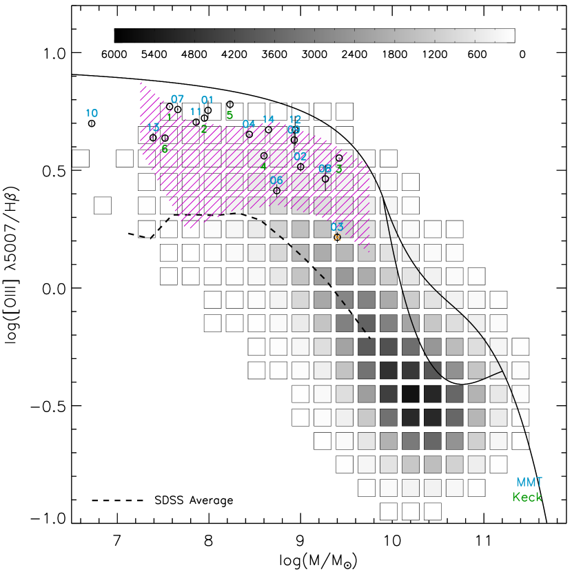
Figure 4.— The MEx diagram for our [O iii]-A sample (circles) plotted against the SDSS DR7 emission-line sample (grey boxes). Each of our galaxies is labelled by a two-digit (MMT; blue) or one-digit (Keck; green) number. The stellar masses are determined from SED fitting, discussed in Section 4.4. The solid black lines defined by Juneau et al. (2011) separate star-forming (left), AGN (right), and composite (middle) galaxies. All of our galaxies are classified as star-forming based on the MEx classification. Our ELGs have [O iii]/H$\beta$ fluxes that are 0.2–0.5 dex higher than the average for SDSS galaxies with the same stellar mass. We also show the SDF spectroscopic sample of $\sim$200 $z=0.4$–1 galaxies in purple with the shaded region representing $\pm$1$\sigma$. This comparison indicates that ELGs at these redshifts have higher ionization in general, across 2.5 dex in stellar mass. Our only LINER (MMT#03) is denoted by the orange cross.

4. RESULTS

In this section, we utilize our spectroscopic and photometric data to estimate dust attenuation (§4.1), electron temperature and gas-phase metallicity (§4.2), de-reddened SFRs (§4.3), stellar properties from SED modeling (§4.4), the local environment (§4.5), and the SFR surface density (§4.6).

4.1. Dust Attenuation Correction from Balmer Decrements

To correct the emission-line fluxes for dust attenuation, we use Balmer decrement measurements obtained from a combination of our spectroscopy and NB imaging. Since our ELGs possess high EWs, 12, 18, and 20 galaxies have H$\delta$, H$\gamma$, and H$\beta$ detected at $\gtrsim$5$\sigma$, respectively. In addition, H$\alpha$ measurements are available for 5 galaxies. Two of them (MMT#10 and MMT#11) are at lower redshifts, allowing us to use their spectroscopic H$\alpha$ measurements. For the other 3 galaxies (MMT#04, #06, #11), the NB H$\alpha$ flux is determined using the following equation:

$$F_{{\rm H}\alpha}=\Delta{\rm NB}\frac{f_{\lambda,{\rm NB}}-f_{\lambda,{\rm BB}}}{1-(\Delta{\rm NB}/\Delta{\rm BB})}f_{\rm corr},$$ (6)

where $f_{\lambda,{\rm NB}}$ and $f_{\lambda,{\rm BB}}$ are the flux density in erg s^-1 cm^-2 Å^-1 for the narrow-band and broad-band, $\Delta$’s are the respective FWHM of the filters ($\Delta z$′ = 956Å), and $f_{\rm corr}$ is the correction for the non-tophat shape of the NB filter when the redshifted H$\alpha$ emission is in the filter’s wing. Using filter throughputs and spectroscopic redshifts, we are able to determine $f_{\rm corr}$. We note that for four galaxies (MMT#03, #07, #13, and #14), the NB fluxes are not reliable for Balmer decrement determinations. In particular, MMT#03 suffers from significant [N ii] contamination in the NB921 filter as a LINER candidate. For the other three sources, the H$\alpha$ line falls in the wing of the NB921 or NB973 filter where precise filter response corrections cannot be made.

A significant problem encountered with using Balmer decrements to determine dust attenuation is the underlying stellar absorption. In three galaxies (MMT#03, MMT#04, and Keck#3), the spectra are of high S/N to sufficiently detect the continuum and fit and remove the stellar absorption or use iraf’s splot command to re-measure the continuum from the absorption trough. For MMT#03 (Keck#3), we determine corrections of EW_abs(H$\delta$) = 2.7Å (1.6Å), EW_abs(H$\gamma$) = 1.9Å (2.5Å), and EW_abs(H$\beta$) = 1.6Å (0.0Å). While for MMT#04, we measure EW_abs(H$\delta$) = 3.9Å and EW_abs(H$\gamma$) = 2.5Å.

For the remaining galaxies, the S/N of our spectra are not sufficient to model the stellar absorption. To correct these galaxies, we adopt EW_abs(H$\delta$) = 2Å and EW_abs(H$\gamma$) = 1Å. We assume no stellar absorption for H$\beta$ and H$\alpha$, which is reasonable since the measured rest-frame emission-line EWs are significantly large (H$\beta$: median of 60Å, average of 95Å).

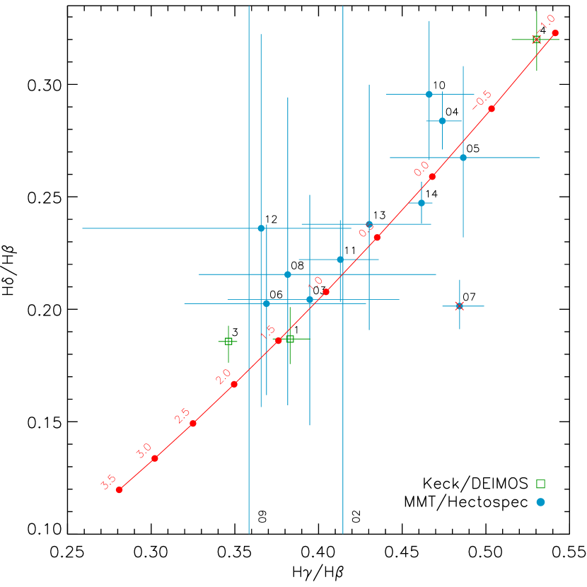
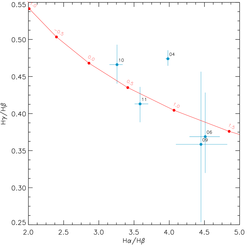
Figure 5.— Balmer decrements for our [O iii] $\lambda$4363 galaxies. The MMT and Keck samples are shown as blue circles and green squares, respectively. Red crosses indicate that the H$\delta$ fluxes are unreliable since it fell on an OH sky-line for MMT#07 and Keck#4. Vertical blue lines indicate non-detections in H$\delta$ for MMT#02 and MMT#09. Finally, red circles and the solid red curves show the effects on the Balmer decrements with increasing dust reddening following C00. The values reported in red are $A$(H$\alpha$).

With these corrections for stellar absorption, we illustrate the Balmer decrements in Figure 5. In addition, we report in Table 4 the absorption-corrected Balmer decrements, and the determined or assumed EW for stellar absorption.

Under the assumption that the hydrogen nebular emission originates from an optically thick ionization-bounded H ii region obeying Case B recombination, the intrinsic Balmer flux ratios are: (H$\alpha$/H$\beta$)₀ = 2.86, (H$\gamma$/H$\beta$)₀ = 0.468, and (H$\delta$/H$\beta$)₀ = 0.259 for $T_{e}$ = 10⁴ K and electron density of $n_{e}$ = 100 cm^-3 (see Section 4.2 for further discussion). We note that these values differ by less than 5% for $T_{e}$ = $2\times 10^{4}$ K. Dust absorption alters these observed ratios:

$$\frac{({\rm H}n/{\rm H}\beta)_{\rm obs}}{({\rm H}n/{\rm H}\beta)_{0}}=10^{-0.4E(B-V)[k({\rm H}n)-k({\rm H}\beta)]},$$ (7)

where $E$($B$–$V$) is the nebular color excess, and $k(\lambda)\equiv A(\lambda)$/$E$($B$–$V$) is the reddening curve at $\lambda$. The latter is dependent on the dust reddening “law.” We illustrate in Figure 5 the observed Balmer decrements under the Calzetti et al. (2000) (hereafter C00) dust reddening formalism with $k({\rm H}\alpha)=3.33$, $k({\rm H}\beta)=4.60$, $k({\rm H}\gamma)=5.12$, and $k({\rm H}\delta)=5.39$. We find that our Balmer decrements are consistent with the C00 dust reddening formula. For the remainder of our paper, all dust-corrected measurements adopt C00 reddening.

Our color excesses, which are tabulated in Table 4, are determined using either H$\alpha$/H$\beta$ (#06, #09–#11) or H$\gamma$/H$\beta$ (MMT#02–#05, #08, #12–#14, and Keck#1, #3, and #4). We do not use H$\delta$/H$\beta$ since it is not well measured for the majority of our galaxies. However, the $E$($B$–$V$) estimates from H$\delta$/H$\beta$ are consistent with H$\gamma$/H$\beta$, as indicated in Figure 5. In three galaxies (MMT#04, MMT#05, and Keck#4), the H$\gamma$/H$\beta$ ratios suggests negative reddening, so we adopt $E$($B$–$V$) = 0.0. For four of our galaxies (MMT#01, #07, #5–#6), the dust reddening could not be determined from Balmer decrements. For these galaxies, we assume $E$($B$–$V$) = $0.24\pm 0.21$ mag ($A({\rm H}\alpha)\approx 0.8\pm 0.7$ mag), which is the average of our sample, and is similar to typical reddening found for local galaxies ($A({\rm H}\alpha)=0.8$–1.1; Kennicutt, 1998a). This also agrees with what we found for ELGs at $z\approx 0.4$ (Ly et al., 2012a).

For Keck#2, the H$\beta$ line unfortunately fell at the edge of a CCD gap, so the H$\beta$ flux is not fully measured. However, the H$\gamma$ and H$\delta$ lines are robustly detected (19 and 9$\sigma$). Assuming Case B recombination and no reddening, the H$\gamma$/H$\beta$ and H$\delta$/H$\beta$ Balmer decrements yielded H$\beta$ fluxes of $2.54\times 10^{-17}$ and $2.87\times 10^{-17}$ erg s^-1 cm^-2, respectively. This excellent agreement in predicted H$\beta$ fluxes suggests that very little reddening is present in this galaxy. We assume $E$($B$–$V$) = 0.0.

Table 4Balmer Decrement Measurements and Derived Reddening

ID	H$\alpha$/H$\beta$	H$\gamma$/H$\beta$	EW(H$\delta$)	EW(H$\gamma$)	EW(H$\beta$)	Source	$E$($B$–$V$)
(1)	(2)	(3)	(4)	(5)	(6)	(7)	(8)
MMT#01	…	…	2.0	1.0	0.0	…	0.24${}^{+0.21}_{-0.21}$string
MMT#02	…	0.41${}^{+0.03}_{-0.04}$	2.0	1.0	0.0	H$\gamma$/H$\beta$	0.25${}^{+0.20}_{-0.22}$string
MMT#03	…	0.39${}^{+0.04}_{-0.04}$	2.7	1.9	1.6	H$\gamma$/H$\beta$	0.35${}^{+0.26}_{-0.24}$string
MMT#04	3.98${}^{+0.04}_{-0.03}$	0.47${}^{+0.01}_{-0.01}$	3.9	2.5	0.0	H$\gamma$/H$\beta$	0.00${}^{+0.05}_{-0.04}$
MMT#05	…	0.49${}^{+0.05}_{-0.04}$	2.0	1.0	0.0	H$\gamma$/H$\beta$	0.00${}^{+0.21}_{-0.21}$
MMT#06	4.51${}^{+0.16}_{-0.18}$	0.37${}^{+0.06}_{-0.05}$	2.0	1.0	0.0	H$\alpha$/H$\beta$	0.39${}^{+0.04}_{-0.03}$string
MMT#07	…	0.48${}^{+0.02}_{-0.02}$	2.0	1.0	0.0	…	0.24${}^{+0.21}_{-0.21}$string
MMT#08	…	0.38${}^{+0.05}_{-0.05}$	2.0	1.0	0.0	H$\gamma$/H$\beta$	0.42${}^{+0.43}_{-0.45}$string
MMT#09	4.45${}^{+0.45}_{-0.44}$	0.36${}^{+0.10}_{-0.10}$	2.0	1.0	4.4	H$\alpha$/H$\beta$	0.38${}^{+0.09}_{-0.10}$string
MMT#10	3.26${}^{+0.08}_{-0.11}$	0.47${}^{+0.04}_{-0.04}$	2.0	1.0	0.0	H$\alpha$/H$\beta$	0.11${}^{+0.02}_{-0.02}$string
MMT#11	3.59${}^{+0.12}_{-0.12}$	0.41${}^{+0.03}_{-0.02}$	2.0	1.0	0.0	H$\alpha$/H$\beta$	0.19${}^{+0.03}_{-0.03}$string
MMT#12	…	0.37${}^{+0.07}_{-0.11}$	2.0	1.0	0.0	H$\gamma$/H$\beta$	0.51${}^{+0.72}_{-0.46}$string
MMT#13	…	0.43${}^{+0.05}_{-0.05}$	2.0	1.0	0.0	H$\gamma$/H$\beta$	0.17${}^{+0.26}_{-0.24}$string
MMT#14	…	0.46${}^{+0.01}_{-0.01}$	2.0	1.0	0.0	H$\gamma$/H$\beta$	0.03${}^{+0.03}_{-0.03}$string
Keck#1	…	0.38${}^{+0.01}_{-0.01}$	2.0	1.0	0.0	H$\gamma$/H$\beta$	0.41${}^{+0.07}_{-0.07}$string
Keck#2	…	…	2.0	1.0	0.0	…	0.00
Keck#3	…	0.35${}^{+0.01}_{-0.01}$	1.6	2.6	0.0	H$\gamma$/H$\beta$	0.62${}^{+0.04}_{-0.04}$string
Keck#4	…	0.53${}^{+0.01}_{-0.01}$	2.0	1.0	0.0	H$\gamma$/H$\beta$	0.00${}^{+0.07}_{-0.07}$
Keck#5	…	…	2.0	1.0	0.0	…	0.24${}^{+0.21}_{-0.21}$string
Keck#6	…	…	2.0	1.0	0.0	…	0.24${}^{+0.21}_{-0.21}$string

.

Note. — Uncertainties are reported at the 68% CL. Stellar absorption line corrections are reported in Cols. (4)–(6)

4.2. $T_{e}$ and Metallicity Determinations

To determine the gas-phase metallicity for our galaxies, we use the empirical relations of Izotov et al. (2006a). This follows the approach of most direct metallicity studies. The first equation estimates $T_{e}$([O iii]) using the nebular-to-auroral [O iii] flux ratio:

$$\log{\left(\frac{[{\rm O}~{}\textsc{iii}]\,\lambda\lambda 4959,5007}{[{\rm O}~{}\textsc{iii}]\,\lambda 4363}\right)}=\frac{1.432}{t_{3}}+\log{C_{T}},$$ (8)

where $t_{3}$ = $T_{e}$([O iii])/$10^{4}$ K,

$$C_{T}=(8.44-1.09t_{3}+0.5t_{3}^{2}-0.08t_{3}^{3})\frac{1+0.0004x}{1+0.044x},$$ (9)

and $x=10^{-4}n_{e}t_{3}^{-0.5}$. For the majority of our galaxies, the [S ii] $\lambda\lambda$6717,6732 doublet, an estimate for $n_{e}$, is redshifted out of our spectral coverage. For one of our galaxies, MMT#10, both [S ii] lines are weakly detected. The $\lambda$6717/$\lambda$6732 flux ratio of $\approx$1.1 corresponds to $n_{e}\approx 400$ cm^-3 (assuming $T_{e}$ = $10^{4}$ K). In addition, DEIMOS has the spectral resolution to separate [O ii] $\lambda\lambda$3726,3729. The $\lambda$3729/$\lambda$3726 flux ratios vary between 0.87 and 1.35, which correspond to $n_{e}=70$–600 cm^-3. To determine $T_{e}$, we assume $n_{e}$ = 100 cm^-3. We note that $C_{T}$ is only affected by $n_{e}$ in the high density regime ($n_{e}\gtrsim 10^{4}$ cm^-3), and therefore assuming $n_{e}$ = 10, 100, or 10³ cm^-3 yields nearly identical $T_{e}$.

We correct the nebular-to-auroral [O iii] flux ratio for dust attenuation using our dust attenuation prescriptions (see Section 4.1). Correcting for dust attenuation increases estimates of $T_{e}$, since dust extincts shorter wavelengths (e.g., 4363Å) more than longer wavelengths (e.g., 5007Å).

In addition, it has been known that $T_{e}$ determinations using (1) various direct metallicity prescriptions, including Izotov et al. (2006a); and (2) strong-line metallicity diagnostics do not yield consistent results (Kewley & Ellison, 2008). These discrepancies have been recently explored, and it is believed that outdated effective collision strengths for the various O⁺⁺ excitation states, and a non-equilibrium distribution of the electron energies result in overestimation of the electron temperature (Nicholls et al., 2012, 2013). Those authors provided applicable corrections for each method. We adopt their corrections, which correspond roughly to a 5% reduction for $T_{e}$ estimates using the Izotov et al. (2006a) approach.

For the very strong ELGs we are studying, our [O iii] measurements have a very large dynamic range. The strongest [O iii] $\lambda$4363 line is as much as 0.089 of the [O iii] flux (MMT#03), while the weakest is 0.007 (Keck#3). We find that the average and median $\lambda$4363/$\lambda$5007 flux ratio for our sample are both 0.037. The derived electron temperatures for our galaxy sample, also have a wide range, from 10⁴ K to $4.5\times 10^{4}$ K. Among our 19 galaxies, 11 have $T_{e}$ estimates of 10⁴–$2.1\times 10^{4}$ K, which are similar to those measured in local galaxies. The large tail toward high $T_{e}$ yields an average $\log(T_{e}/{\rm K})$ that is higher than the average of local galaxies by 0.15 dex.

Other higher redshift studies have measured high $T_{e}$ in star-forming galaxies. For example, Yuan & Kewley (2009) detected [O iii] $\lambda$4363 in a lensed $z=1.7$ galaxy and measured $T_{e}$ $\approx 2.35\times 10^{4}$ K, and Hu et al. (2009) have also measured large [O iii] $\lambda$4363/$\lambda$5007 flux ratios in a few ELGs. The higher values of $T_{e}$ are not well-determined, and have a large tail (0.2–0.3 dex) toward lower temperatures. This is likely the case for other published measurements, as Yuan & Kewley (2009) yielded a 3$\sigma$ detection of [O iii] $\lambda$4363 and the measurement uncertainties of Hu et al. (2009) result in a significant tail toward low $T_{e}$.

MMT#03 has the most extreme $T_{e}$ value, but as we mentioned in Section 3.1, it is a LINER with shock-heated, rather than photo-ionized gas producing most of its emission-line spectrum. Other galaxies with high $T_{e}$ ($\gtrsim 2.5\times 10^{4}$ K) are MMT#06, #08, #09, #12, Keck#5, and #6. To examine if these temperatures are reasonable, we generate low-metallicity models with CLOUDY (Ferland et al., 1998). In our modeling, we input Starburst99 (Leitherer et al., 1999) SEDs that adopt Geneva stellar evolution models with five stellar metallicities between $Z$/$Z_{\sun}$ = 0.05 and 2.0. Coupling the stellar and gas metallicity, we find that the highest plausible $T_{e}$([O iii]) temperature is $\approx$25,000 K for $Z$/$Z_{\sun}$ = 0.02–0.03. Given this upper limit, we fix the dust-corrected $T_{e}$([O iii]) to not exceed this temperature for these six galaxies. We note that without this $T_{e}$ offset, the resulting oxygen metallicity will be lower by 0.1–0.4 dex for these six galaxies.

The $T_{e}$ measurements for all 20 objects are shown in Figure 6. Throughout this paper, we generate realizations of the emission-line fluxes to construct probability distribution functions (PDFs) for all observed and derived measurements. This is critical, as the distributions are non-Gaussian in the domain of low S/N ($\lesssim$5), and it allows us to propagate our measurement uncertainties, including $E$($B$–$V$).

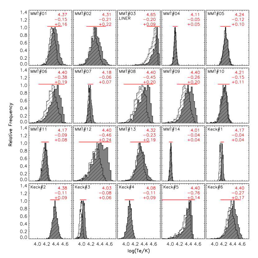
Figure 6.— Probability distribution functions for the electron temperature determined from the [O iii] $\lambda$4363 line. The peak values and $\pm$95% confidences are reported in each panel. $T_{e}$’s are derived from the observed flux ratios (hashed histograms) and the dust-corrected flux ratios (grey histograms).

To determine the ionic abundances of oxygen, we use two emission-line flux ratios, [O ii] $\lambda\lambda$3726,3729/H$\beta$ and [O iii] $\lambda\lambda$4959,5007/H$\beta$:

$$12+\log{\left(\frac{{\rm O}^{+}}{{\rm H}^{+}}\right)}=\log{\left(\frac{[{\rm O}~{}\textsc{ii}]}{{\rm H}\beta}\right)}+5.961+\frac{1.676}{t_{2}}$$ (10)

$$-0.4\log{t_{2}}-0.034t_{2}+\log{(1+1.35x)}$$

$$12+\log{\left(\frac{{\rm O}^{++}}{{\rm H}^{+}}\right)}=\log{\left(\frac{[{\rm O}~{}\textsc{iii}]}{{\rm H}\beta}\right)}+6.200+\frac{1.251}{t_{3}}$$ (11)

$$-0.55\log{t_{3}}-0.014t_{3}.$$

Here, $t_{2}$ refers to the singly-ionized oxygen electron temperature, $T_{e}$([O ii]). For our metallicity estimation, we adopt a standard two-zone temperature model with $t_{2}\equiv$ $T_{e}$([O ii])/10⁴ K = $-0.577+t_{3}(2.065-0.498t_{3})$ (Izotov et al., 2006a). In computing O⁺/H⁺, we also correct the [O ii]/H$\beta$ ratio for dust attenuation. We do not correct O⁺⁺/H⁺ since the effects are negligible (e.g., the [O iii]/H$\beta$ ratio changes by less than 0.02 dex for $A$(H$\alpha$) = 1 mag).

Since the most abundant ions of oxygen in H ii regions are O⁺ and O⁺⁺, we can determine the oxygen abundances as:

$$\frac{\rm O}{\rm H}=\left(\frac{\rm O^{+}}{\rm H^{+}}\right)+\left(\frac{\rm O^{++}}{\rm H^{+}}\right).$$ (12)

In Table 5, we provide observed and de-reddened flux ratios, estimates of $T_{e}$([O iii]), $\log({\rm O^{+}/H^{+}})$, $\log({\rm O^{++}/H^{+}})$, and 12 + $\log({\rm O/H})$ for our sample, and 95% confidence uncertainties (i.e., two standard deviations). In addition, we illustrate our PDFs of 12 + $\log({\rm O/H})$ in Figure 7. Our three most metal-poor galaxies are MMT#13, Keck#2 and #6 with 12 + $\log({\rm O/H})$ = 7.53${}^{+0.52}_{-0.33}$, 7.54${}^{+0.27}_{-0.22}$, and 7.24${}^{+0.45}_{-0.30}$, respectively. For our sample of 19 star-forming galaxies, 4 of them can be classified as an XMPG as their metallicity is below 12 + $\log({\rm O/H})$ = 7.65.

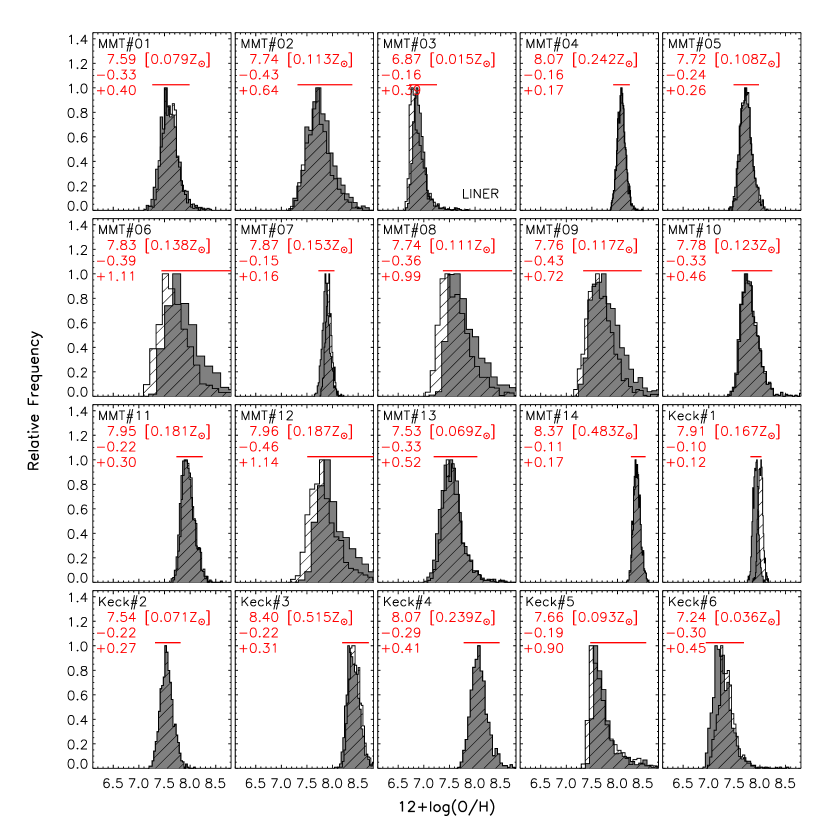
Figure 7.— Probability distribution functions for the gas-phase metallicity, 12 + $\log({\rm O/H})$. The peak values and $\pm$95% confidences are reported in each panel. We illustrate the observed and de-reddened determinations by the hashed and grey filled histograms, respectively. The upper limit of the [O ii] flux is adopted for calculating the metallicity for Keck#6.

4.3. Dust-Corrected Star Formation Rates

In addition to gas-phase metallicity determinations, our extensive data allow us to determine dust-corrected SFRs using the Hydrogen recombination lines, which are sensitive to the shortest timescale of star formation, $\lesssim$10 Myr (i.e., an instantaneous SFR estimate).

Assuming a Chabrier (2003) (hereafter Chabrier) initial mass function (IMF) with minimum and maximum masses of 0.1 and 100 $M_{\sun}$, and solar metallicity (Kennicutt, 1998a), the SFR can be determined from the dust-corrected H$\alpha$ luminosity as:

$${\rm SFR}(M_{\sun}~{}{\rm yr}^{-1})=4.4\times 10^{-42}L({\rm erg~{}s}^{-1}).$$ (13)

Similarly, SFRs can be determined from H$\beta$ by first correcting for dust reddening ($A$(H$\beta$) = 4.60 $E$($B$–$V$)), and then adopting the intrinsic Case B flux ratio, (H$\alpha$/H$\beta$)₀ = 2.86.

Our SFR estimates are summarized in Table 6 and illustrated in Figure 8. We find that our galaxies have dust-corrected SFRs of 0.04–64 $M_{\sun}$ yr^-1 with an average (median) of 8.1 (2.3) $M_{\sun}$ yr^-1.

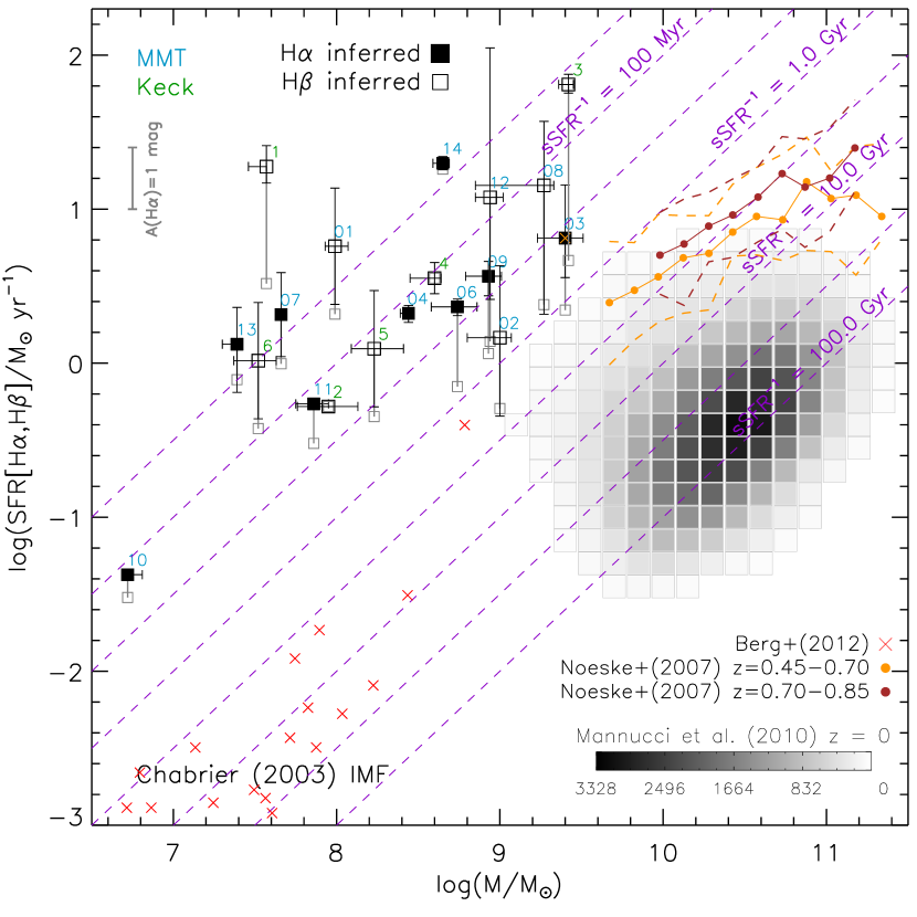
Figure 8.— The SFR versus stellar mass for our [O iii]-A sample. The stellar masses are obtained from SED fitting (Section 4.4) where we adopt a Chabrier IMF. The SFRs are determined from either H$\alpha$ (filled squares) or H$\beta$ (open squares), which are sensitive to a timescale of $\lesssim$10 Myr. The observed SFRs are shown as grey open squares with the degree of dust attenuation corrections indicated by the solid grey vertical lines. These dust corrections are discussed further in Section 4.1. The average (median) sSFR of our galaxies is $10^{-8}$ yr^-1 ($8\times 10^{-9}$ yr^-1). Each of our galaxies are labelled by a two-digit (MMT; blue) or one-digit (Keck; green) number. Our only LINER (MMT#03) is denoted by the orange cross. Overlaid in red crosses are the low-luminosity local sample of Berg et al. (2012), and the greyscale demonstrates the SDSS sample used by Mannucci et al. (2010). The “main sequence” relation of Noeske et al. (2007) at $z=0.45$–0.7 and $z=0.7$–0.85 are illustrated in orange and brown, respectively. For direct comparisons, we have corrected Noeske et al. (2007) and Berg et al. (2012) measurements to a Chabrier IMF.

4.4. Spectral Energy Distributions and Estimated Stellar Population Properties

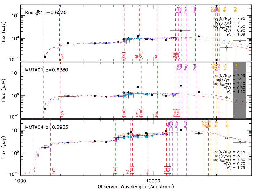
Figure 9.— The SED and the best-fitting stellar population results from modeling the SED in three galaxies: Keck#2, MMT#01, and #04. The observed fluxes are shown by the black circles while the blue circles illustrate the corrections for nebular emission lines. Errorbars along the $x$-axis demonstrate the FWHM of the filters while those along the $y$-axis are 1$\sigma$. The best $\chi^{2}$ fits to the original and emission-line corrected SEDs are shown in red and blue, respectively. In fitting the SED, we exclude the IRAC photometry, but include them in this figure for comparison. The emission-line corrected fitting results are reported on the right. Grey vertical lines indicate the locations of the Balmer and Lyman continuum breaks, while red, purple, and orange vertical lines show the location of various redshifted emission lines. When correcting for emission lines, the $\chi^{2}$ values are reduced by a factor of 3.5–10.3 in these three cases. In MMT#04, we find that the stellar mass and age are overestimated by 0.3 dex and 0.7 dex, respectively.

One significant advantage of studying low-mass galaxies in the SDF is the ultra-deep imaging in twenty-four bands from the UV to the IR, which allows us to characterize their stellar properties. The SDF is imaged with: (1) GALEX (Martin et al., 2005) in both the FUV and NUV bands; (2) KPNO’s Mayall using MOSAIC in $U$; (3) Subaru with Suprime-Cam in 14 bands ($BVR_{\rm C}i\arcmin z\arcmin z_{b}z_{r}$, and the five NB and two IA filters as mentioned previously); (4) KPNO’s Mayall using NEWFIRM (Probst et al., 2008) in $J$ and $H$, (5) UKIRT using WFCAM in $K$, and (6) Spitzer in the four IRAC bands (3.6$\mu$m, 4.5$\mu$m, 5.8$\mu$m, and 8.0$\mu$m). As discussed in Ly et al. (2011a), a more complete photometric catalog from SExtractor was constructed from an ultra-deep mosaic that consisted of stacked optical and near-IR images with a normalization that takes into account the rms (i.e., $\chi^{2}$ stacking).

Upon cross-referencing our 20 galaxies with the complete photometric sample, all but one of them have direct matches. The missing source (MMT#05) was confused with a nearby bright extended galaxy. We exclude MMT#05 in our stellar population analyses. For the remaining 19 galaxies, aperture photometry measurements in 15 bands from the FUV to $K$ are used to construct their complete broad-band SEDs. There are two modifications that we make to these measurements.

First, since all our galaxies are virtually point sources for GALEX, we obtain more accurate photometry in the FUV and NUV bands by PSF-fitting with daophot (Stetson, 1987). Our examination of the residuals for each source suggests that the PSF-fitting is extremely successful, and that these galaxies are not affected by contamination of nearby sources. Among the Keck sample, we note that only Keck#2 is detected in the FUV. The lack of FUV detections is un-surprising, since the Lyman continuum break occurs redward of the filter for the remaining five Keck sources. Also, Keck#6 is not detected in the NUV because of its intrinsic faintness. Because the MMT [O iii] $\lambda$4363 galaxies are brighter with $z\lesssim 0.65$, they are all detected in the NUV and FUV bands, allowing for robust UV SFR determinations.

Second, since our galaxies all have very high emission-line EWs, we correct the broad-band photometry for the contribution from nebular emission lines using emission-line measurements from our spectroscopy and NB imaging. Here we generate a spectrum for each galaxy with zero continuum and emission lines located at the redshifted wavelengths for [O ii], [Ne iii], H$\beta$, [O iii], H$\alpha$, and higher order Balmer lines. These spectra are then convolved with the filter bandpasses to determine excess fluxes, and then are removed from the broad-band photometry. The correction for emission lines to SEDs has been recently explored in other higher redshift studies where high-sSFR galaxies are more prominent at $z\gtrsim 1$ (Atek et al., 2011; Pirzkal et al., 2013). For two galaxies (MMT#10 and MMT#11), the redshifts are low enough to have spectroscopic detections of H$\alpha$. For a subset of MMT galaxies (#03, #04, #06, #07, #09, #13, and #14), we use the NB921 or NB973 excess fluxes for H$\alpha$ flux estimates. However, for galaxies at $z\geq 0.5$ and $0.43\lesssim z\lesssim 0.47$, H$\alpha$ is redshifted into the near-IR or not available from optical spectroscopy. To correct H$\alpha$ in these galaxies (Keck#1–#6, MMT#1, #2, #8, and #12), we use spectroscopic information for H$\beta$, but with the assumption that H$\alpha$ is three times stronger. Of course, higher dust reddening will yield stronger H$\alpha$ corrections, so we are adopting a minimum correction of $A({\rm H}\alpha)$ = 0.14 mag.

Both our observed SEDs and those corrected for nebular emission lines are tabulated in Table 7, and representative examples are shown in Figure 9. The black circles show the original broad-band photometry, while the blue circles show the corrected continuum fluxes after removal of emission lines. These three examples illustrate how the SEDs change when the emission-line corrections are small, average, and among the largest.

Both the original and corrected SEDs were fitted with stellar population synthesis models (Bruzual & Charlot, 2003) with the Fitting and Assessment of Synthetic Templates (FAST; Kriek et al., 2009) code. We use exponentially-declining star formation histories (i.e., $\tau$ models) similar to previous fitting by us and many other groups (Ly et al., 2011a). We have chosen this star-formation history (SFH) for its simplicity since broad-band data are generally unable to distinguish against more complicated SFHs (e.g., a constant SFR with a recent burst, which may be more representable for our galaxies). As we later find, these fits adopting an exponentially declining SFH are consistent with the data with nearly unity $\chi^{2}_{\nu}$ values. Also, the primary purpose of our SED modeling is to obtain stellar masses of our galaxies. This is best traced from the rest-frame optical light from the older stellar population. Thus the inclusion of a recent burst does not significantly alter stellar mass estimates.

In these models, we continue to adopt C00 reddening, and inter-galactic medium attenuation following Madau (1995). The only differences are that we adopt a Chabrier IMF, allow for an extremely short burst model, $\tau=10^{7}$ yr, and use stellar atmospheres with one-fifth ($Z$=0.004) solar abundances. The latter is motivated by the fact that our galaxies are extremely metal-poor. In addition we considered solar abundance ($Z$=0.02) for completeness. We find that for the majority of our galaxies, the $Z$=0.004 models yield similar results to $Z$=0.02 models. For consistency with our metallicity determinations, we adopt the SED fitting results with $Z$=0.004 models.

We find that with the emission-line corrections, the SED fits are improved with lower $\chi^{2}$ values by a factor 1.1–10.4 in the $Z$=0.004 models with an average (median) improvement of 3.3 (2.1). In general, the results of fitting the SEDs with emission-line corrections yielded lower stellar masses by 0.1 dex and younger ages by 0.1 dex on average. However, these differences vary from one source to another. In particular, our analyses also reveal a moderate correlation between [O iii] EW and the difference in stellar mass determinations, which others have reported (Atek et al., 2011).

Our SED-fitting results are summarized in Table 6. We find that these galaxies typically are low-mass systems (median of $3\times 10^{8}$ $M_{\sun}$, average of $2\times 10^{8}$ $M_{\sun}$). However, there is dispersion in the mass distribution (extending from $5\times 10^{6}$ to $3\times 10^{9}$ $M_{\sun}$). The estimated light-weighted stellar ages of $\log{(t_{\rm age}/{\rm yr})}=7.1$–8.7 dex (average: 7.75 dex) suggest that these galaxies have undergone most of their star formation in the recent past.

We compare the de-reddened SFRs estimated from SED fitting against the Balmer-derived de-reddened SFRs and find good agreement, albeit with large uncertainties. We also compare the dust reddening determinations from SED fitting and Balmer decrements and find a weak correlation. With large uncertainties in determining reddening with both methods, it is not possible for us to investigate any difference between nebular and stellar reddening. The weak correlation is consistent with $E$($B$–$V$)${}_{\rm gas}\approx 1.5$$E$($B$–$V$)_star. This result is similar to what we found for a larger sample of ELGs in Ly et al. (2012a).

Finally, we combine our dust-corrected SFRs (Section 4.3) and stellar mass determinations to illustrate our galaxies on the SFR–$M_{\star}$ plane in Figure 8. Relative to their stellar mass, we find that our ELGs are all undergoing strong star formation. In particular, the sSFRs are between $10^{-9}$ yr^-1 and $7\times 10^{-7}$ yr^-1 with an average of $10^{-8}$ yr^-1. This is 2.0–3.0 dex higher than the so called “main sequence” of star formation for $z\sim 0$ SDSS galaxies (Mannucci et al., 2010) and low-luminosity local galaxies (Berg et al., 2012). Extrapolating the main sequence of Noeske et al. (2007) toward lower stellar mass, we find that the sSFR of our ELGs are $\approx$0.5–1.0 dex higher than “typical” galaxies at $z\sim 0.45$–0.85, but they are consistent with Noeske et al. (2007)’s sample at the 1$\sigma$ level. We emphasize that the inverse of the sSFRs, is consistent with the stellar ages derived from SED fitting.

With the strong nebular emission lines seen in our galaxies, the nebular continuum from free-free, free-bound, and two-photon emissions can be important (see e.g., Izotov et al., 2011). To estimate the contribution toward the total light, at rest-frame optical wavelength, we generate spectral synthesis models from Starburst99. In our models we assume a constant SFH, a Kroupa (2001) IMF, Geneva stellar evolutionary models, and $Z$/$Z_{\sun}$ = 0.05. For EW₀(H$\beta$) = 45Å (the median of our sample), we estimate that the nebular continuum is responsible for $\lesssim$10% of the total optical/IR light, and thus the stellar masses (sSFRs) that we have reported are $\lesssim$0.05 dex overestimated (underestimated). We note that this correction can be as large as 20–50% (0.1–0.3 dex) in galaxies (Keck#1, MMT#07) with EW₀(H$\beta$) of $\approx$250–400Å. However, these corrections for only two galaxies do not significantly alter our MZR.

4.5. Nearby Emission-line Galaxy Companions

Utilizing our deep NB/IA images, we constructed postage stamps that contain only the emission-line excess flux by differencing the NB/IA images with adjacent broad-band images (as previously discussed in Section 2.1). For proper removal of the continuum, we normalize the images by their respective zeropoints. We find that the majority (14 of 20) of our sample has between 1 and 4 NB/IA excess emitters within a projected radius of $\approx$100 kpc. The closest separation is 12 kpc with an average projected distance of 48 kpc.

To ensure that these nearby NB/IA excess sources are real, we conducted two checks. First, we examine if any of these nearby galaxies are also classified as an NB/IA excess emitter in our source catalogs. We find that more than half of them (16 of 34) are NB/IA excess emitters. Upon further inspection, we find that those that are missed did not satisfy our NB/IA excess selections because they have low emission-line EW or are faint, but many could also lie at the same redshift as our [O iii] $\lambda$4363 galaxies. Second, some of our galaxies are identified as an excess emitter in two or more filters (e.g., NB704 and NB921). This is due to multiple emission lines falling in these filters. We find that in these four galaxies, six of the nearby excess emitters are also detected in two or three filters. This result strongly suggests that these nearby NB/IA excess emitters surrounding our [O iii] $\lambda$4363-selected galaxies are physically real, and at a similar redshift.

While our sample size is small, the presence of nearby ($\lesssim$100 kpc) companions in 70% of our galaxies suggests that this is unlikely to be a coincidence. To confirm this, we examine how frequent nearby emission-line companions are using our sample of 401 $z=0.4$ H$\alpha$ emitters, which has been previously discussed in Ly et al. (2012a). We determine the projected distance to the nearest H$\alpha$ emitter, and find that the average of this distance is $\approx$350 kpc (median is $\approx$280 kpc). Furthermore we find only 49 of 401 (12%) H$\alpha$ emitters have a companion that is within 100 kpc. This low percentage suggests that H$\alpha$ emitters, while clustered, are infrequently found with a nearby satellite. An identical analysis with 715 $z=0.84$ [O iii] emitters yielded similar numbers.

Three plausible explanations for the significant excess of nearby companions are that galaxy-galaxy interactions can: (1) stimulate a “starburst”, (2) tidally strip out metal-rich gas into the CGM, or (3) cause accretion of metal-poor gas from the outskirts of the galaxy.

In the first case, the intense star formation can trigger strong winds that can entrain metal-rich gas into the CGM. If so, this would explain why these galaxies are identified to be extremely metal-deficient. Our measurements of SFR and masses (see Figure 8) suggest that the current SFR could form most of the stellar population in $\sim$100 Myr (average), supporting this hypothesis. Since our [O iii] $\lambda$4363 sample is inhomogenous (i.e., selection in different NB/IA filters), a more detailed study is warranted from the complete NB/IA sample. Forthcoming work will examine further these nearby companions and any correlation seen with the properties of the central galaxies.

In the case of “tidal disruption,” one would expect to see evidence of gas stripping, in the form of tidal tails and asymmetric morphologies. An examination of our NB/IA-excess images reveal no tidal tails or any “bridge” between our targeted sources and a nearby companion. We do notice that the light distribution is asymmetric in half of our galaxies; however, the seeing-limited resolution of our data makes it difficult to interpret such results. Higher resolution imaging with Hubble Space Telescope (HST) is needed to quantitatively measure the morphological properties of these galaxies and detect any tidal tail features.

One of our galaxies (Keck#05) fortuitously has HST/WFC3 broad-band near-IR imaging (Jiang et al., 2013). Keck#05 is in fact two galaxies that are separated along the NE–SW direction by 0.9″ (projected distance of 6.9 kpc at $z=0.84$) with the nebular emission coming from the SW component. Our examination of the HST imaging reveal that the NE galaxy is diffuse along the P.A. toward the SW component. More careful analysis is needed to understand Keck#05 and its nearby companion, and as we emphasized, HST imaging for a larger fraction of our [O iii]-A sample is required to examine the possibility of tidal disruption for the case of low metallicities in our galaxies. We note however that this scenario is unlikely to result in low metallicity in the centers of these galaxies, as these dynamical effects are expected to have a stronger impact on the gas that is external to the galaxy, which is relatively more metal-poor, than the metal-rich gas that is located closer to the center.

Another contrasting possibility is that the interaction with the nearby galaxy induces gravitational torques that drive metal-deficient gas from the outskirts of galaxies into the centers (e.g., Mihos & Hernquist, 1996). Support for this idea has been seen in local interacting galaxies where the radial metallicity gradient is unusually flat (Kewley et al., 2006; Rupke et al., 2010). This would explain (1) the deficiency of metals, (2) the excess of nearby galaxies, and (3) the high SFRs and SFR surface densities (see Section 4.6) in our galaxies.

Our data do not decisively distinguish between these models without dynamical information. In particular, IFU spectroscopy of the ionized gas would reveal the presence of inflowing or outflowing gas.

4.6. Star Formation Surface Densities

In addition to subtracting of the continuum to identify nearby companions, the NB/IA excess flux images allow us to determine their SFR surface density, $\Sigma_{\rm SFR}$. These images are first converted to an emission-line luminosity, then integrated across the galaxy to determine a total H$\alpha$ or H$\beta$ observed luminosity, and finally corrected for dust attenuation (Section 4.1). Six of our galaxies (MMT#04, #06, #07, #09–#11) have NB imaging or spectroscopy that observes H$\alpha$. In addition, three other galaxies (MMT#13, #14, and Keck#4) have H$\beta$ measurements. The remaining galaxies (MMT#01, #02, #08, #12, Keck#1, #2, and #5) are [O iii]-selected. To obtain an estimate of the H$\beta$ luminosity for the latter galaxies, we use the integrated [O iii]/H$\beta$ ratio from our spectroscopy (see Table 3). Finally to obtain the H$\alpha$ luminosities, we scale the de-reddened H$\beta$ measurements by a factor of 2.86. We integrate the source flux over a region that is $\pi({\rm FWHM}/2)^{2}$, which is converted to physical distance using the angular diameter distance (1″ = 5.4 kpc at $z=0.4$ and 7.8 kpc at $z=0.85$). This measured area is larger due to the degradation from seeing. To correct for it, we determine the effective FWHM in quadrature: FWHM${}_{\rm eff}^{2}$ = FWHM² - FWHM${}_{\rm seeing}^{2}$. Due to the slightly extended nature of our galaxies, this correction to the area is typically a factor of 2 or less. We find a wide dispersion in the $\Sigma_{\rm SFR}$ between 0.005 and 5 $M_{\sun}$ yr^-1 kpc^-2 with an average (median) of 0.5 (0.04) $M_{\sun}$ yr^-1 kpc^-2. Compared to local galaxies (Kennicutt, 1998b), our $\Sigma_{\rm SFR}$’s are on average an order of magnitude higher than normal spirals, and at the low end of IR-selected circumnuclear starbursts.

5. DISCUSSION

5.1. Our [O iii] $\lambda$4363 Sample

By construction, the 20 galaxies presented in this paper were selected to be extreme. First, our SDF follow-up spectroscopy concentrated on ELGs identified from our NB/IA imaging. Then in this paper we have selected only a few percent of these spectra, where the lines were strong enough to include detectable [O iii] $\lambda$4363. Half of our galaxies were solely targeted because of the strength of their [O iii] $\lambda\lambda$4959,5007 doublet (see Table 1). This favors emission from more highly ionized gas. Although the [O iii] $\lambda$4363 line is occasionally seen in LINERs, we only found one of them based on various emission-line ratios (see Section 3.1). The remaining 19 are all extreme starburst galaxies, which tend to be overlooked by traditional broad-band photometric selections. Aside from deep narrow-band imaging, the only other windows on galaxy evolution which provides access to many extreme SFR galaxies are extensive spectroscopy with as little pre-selection as possible, preferably none (such as slitless spectroscopy; Atek et al., 2010) or selecting galaxies with unusual colors (Cardamone et al., 2009; van der Wel et al., 2011).

Thus these 20 galaxies lie far above the established correlation of star formation rate with stellar mass. In other words, their sSFR is between two and three orders of magnitude larger than the average observed in the local universe, or even than what is “normal” for galaxies at $z=0.4$–0.9. These [O iii] $\lambda$4363-detected galaxies are extremely rare in the local universe, making up only 0.05% of those with SDSS spectra.

Since sSFR is the inverse of the star production time-scale, continuing at their high observed SFRs, our extreme galaxies would produce their entire stellar contents in only 1%–10% of the time it takes in normal galaxies. This strongly suggests that we are observing them in a highly atypical evolutionary phase, which could last 100 Myr or even less. If this is a phase that most galaxies pass through occasionally, then the ‘duty cycle’ of this extreme burst of star formation would be only $\sim$1%–10%.

5.2. Selection Effects

The NB technique has two observable limitations: (1) a minimum EW excess at the bright end ($\lesssim$24 mag), and (2) an emission-line flux limit at the faint end. In the former case, our selections are limited to galaxies with rest-frame EWs of EW₀([O iii]) = 11Å–17Å ($z=0.4$–0.85) and EW₀(H$\alpha$) $\approx$ 20Å ($z=0.24$–0.40). With a 2.5$\sigma$ emission-line flux limit of approximately $4.5\times 10^{-18}$ erg s^-1 cm^-2, the luminosity limit corresponds to $3\times 10^{39}$ and $2\times 10^{40}$ erg s^-1 at $z=0.40$ and $z=0.84$, respectively. These EW and luminosity limits are illustrated in Figure 3, and are compared to the ELGs in the SDSS. It can be seen that our NB imaging cannot detect the [O iii] emission from many SDSS galaxies, simply because of the lower equivalent widths. For example, only 16% of the full SDSS galaxy sample would be identified as NB704 excess emitters at $z=0.40$. However, this fraction increases to 90% for ELGs with moderate line strengths, EW₀([O iii]) $\gtrsim 11$Å. For H$\alpha$, the majority (62%) of the SDSS would be detected at $z=0.4$ with our NB921 imaging, and almost all (96%) of galaxies with EW₀(H$\alpha$) $\gtrsim 22$Å. Thus, our NB survey is biased against weak emission lines. We note that the lower success of detecting [O iii] in SDSS ELGs at $z=0.4$ compared to H$\alpha$ is due to the higher metallicities in local galaxies. In metal-rich systems (i.e., lower $T_{e}$), O⁺ is a more effective coolant for the ISM than O⁺⁺, resulting in flux ratios of [O ii]/H$\alpha$ $\approx 0.5$ and [O iii]/H$\alpha$ $\approx 0.1$. Thus, our [O iii] NB selection is less sensitive to metal-rich galaxies.

In addition to our general NB selection, the primary restriction for our sample is an [O iii] $\lambda$4363 detection. First, this limits the sample toward high-EW galaxies, which generally have high sSFRs. Second, the detection alone will further bias our sample against moderately metal-poor galaxies (12 + $\log({\rm O/H})$ $\approx 8.0$). For example, in our spectroscopic survey, we have identified an additional $\sim$20 galaxies that possess strong [O iii] emission (EW${}_{0}\gtrsim 50$Å). These galaxies, however, have very weak detections of [O iii] $\lambda$4363 (1–3$\sigma$).

While an [O iii] $\lambda$4363 detection restricts our ELG sample, we find that our 20 galaxies have many similarities to our more general ELG sample at $z\approx 0.4$–1. For example, the median (average) stellar mass of our spectroscopic sample of over 200 galaxies is $\log(M_{\star}/M_{\sun})$ = 8.9 (8.7). These values are moderately higher (0.4 dex) than our [O iii]-A sample. Also, as illustrated in Figure 4, our [O iii]-A sample shows similar [O iii]/H$\beta$ ratios, which is a measure of the ionization. This demonstrates that ELGs selected from NB surveys at $z=0.4$–1 all have higher ionization by $\approx 0.2$–0.5 dex compared to local SDSS galaxies with similar stellar masses.

5.3. Similarities and Differences to Green Peas and Luminous Compact Galaxies

The SDSS has found rare populations of strongly star-forming galaxies called “Green Peas” (Cardamone et al., 2009) and “Luminous Compact Galaxies” (LCGs) (Izotov et al., 2011). The former population was identified by unusual optical colors due to significant contribution of very strong nebular emission lines ([O iii] and H$\beta$) in the $r$-band (hence they appear “green”). Ancillary data indicated that these luminous ($r\lesssim 20.5$) galaxies are at $z\approx 0.1$–0.35, have stellar masses of $\sim$10^8.5–10¹⁰ $M_{\sun}$ and SFRs of $\sim$10 $M_{\sun}$ yr^-1, are relatively metal-rich 12 + $\log({\rm O/H})$ $\sim$ 8.7, and are very rare (2 deg^-2). Because of the unusual color selection, selection effects are significant for this sample.

Analogously, LCGs were identified from the SDSS DR7 spectroscopic sample to have EW(H$\beta$) $\gtrsim 50$Å, at least 2$\sigma$ detections of [O iii] $\lambda$4363, and appear compact or unresolved in the SDSS images. These galaxies have redshifts of $z=0.02$–0.63 (most of them are at $z\lesssim 0.35$), median stellar masses of $\sim$10⁹ $M_{\sun}$, median SFRs of $\sim$4 $M_{\sun}$ yr^-1, and oxygen abundance of 12 + $\log({\rm O/H})$ $\approx$ 8.2. Since it is believed that green peas are a subset of LCGs (Izotov et al., 2011), we will only compare our sample against the LCG population.

LCGs show many similarities and differences to our galaxies with [O iii] $\lambda$4363 detections. First, both samples occupy a distinct region in BPT and MEx diagnostics diagrams with large [O iii]/H$\beta$ and low [N ii]/H$\alpha$ (or stellar mass). While LCGs have low stellar masses and high sSFRs, they are on average $\sim$0.5 dex more massive than our sample and with lower sSFR by $\sim$0.5 dex. These LCGs can be found with stellar masses above $10^{10}$ $M_{\sun}$, while our most massive galaxy has $M_{\star}$ $\approx 3\times 10^{9}$ $M_{\sun}$. In addition, these galaxies are relatively metal-rich by $\sim$0.4–0.5 dex compared to our sample. Also, 90% of our [O iii]-A sample is found above $z=0.4$, while the majority of LCGs are identified at $z\lesssim 0.35$. Therefore, while LCGs are low-mass, metal-poor galaxies, our [O iii]-A sample appears to be an extension of LCGs toward lower masses, lower metallicity, and higher redshift. These differences might suggest that metal-poor ELGs identified with deep NB imaging may evolve into LCGs. Finally, in terms of surface density, it is estimated that there are $\approx$20 LCGs per deg². The SDF has already detected [O iii] $\lambda$4363 in 20 galaxies over 0.25 deg², and more of them are expected to be found (see Section 5.6). The higher surface density is because our survey extends toward lower mass galaxies, which are more common, and because higher sSFR are seen for galaxies at higher redshift (see Section 5.6).

5.4. Comparison with Other [O iii] $\lambda$4363 Studies

While these metal-poor galaxies are rare, there have been numerous efforts to identify them. Here, we compare our sample to previous [O iii] $\lambda$4363 studies. Two of the first studies that probed a large number of low-mass galaxies in the local universe were Lee et al. (2004) and Lee et al. (2006). First, Lee et al. (2004) identified and detected [O iii] $\lambda$4363 for 24 local galaxies from the KPNO International Spectroscopic Survey. These galaxies, spanning $M_{B}$ = –15 and –19, were pre-selected to have gas-phase metallicities (determined from strong-line methods) to be below 12 + $\log({\rm O/H})$ = 8.2. The sample provided the first measurement of the MZR using the “direct” method. Targeting 25 dwarf irregular galaxies, Lee et al. (2006) extended the MZR toward lower stellar masses. Since then, more extensive spectroscopy has been conducted targeting low-luminosity galaxies within 11 Mpc (Berg et al., 2012), and mining the SDSS (Brown et al., 2008; Izotov et al., 2006a, 2012a).

In addition, a few other studies have succeeded at extending the search toward higher redshift where the redshift evolution of the MZR implies that more metal-poor galaxies should be found in the early universe. Hoyos et al. (2005) was the first study to detect [O iii] $\lambda$4363 in 17 $\sim$$L_{\star}$ galaxies at $z=0.51$–0.86 with gas metallicity ranging from 12 + $\log({\rm O/H})$ = 7.8–8.3. These galaxies were selected from the DEEP2 Survey (Davis et al., 2003) and TKRS (Wirth et al., 2004), which are luminosity-limited to $I=24.5$ and $R=24.3$ mag, respectively. Then Kakazu et al. (2007) conducted follow-up spectroscopy of ultra-strong ELGs selected from NB imaging. While some level of detection for [O iii] $\lambda$4363 was available in 17 galaxies, only six had $\geq$3$\sigma$ [O iii] $\lambda$4363 detection. The rest were too weak, with a median detection of $\approx 2\sigma$. Among those with robust detections ($\geq$3$\sigma$), their most metal-poor galaxy has 12 + $\log({\rm O/H})$ = $7.36^{+0.22}_{-0.18}$ (1$\sigma$). They have since extended their [O iii] $\lambda$4363 sample to a total of 31 galaxies at $z=0.40$–0.85 (Hu et al., 2009). About three-fourths (23/31) of their sample are detected above 3$\sigma$ with 9 galaxies above 5$\sigma$. Their most metal-poor galaxies have 12 + $\log({\rm O/H})$ = 6.97$\pm$0.17 and 12 + $\log({\rm O/H})$ = 7.25$\pm$0.03 (1$\sigma$).

In addition, Atek et al. (2011) identified a sample of high-EW ELGs at $z=0.35$–2.3 from space-based grism spectroscopy. With higher spectral resolution follow-up observations, they detected [O iii] $\lambda$4363 to determine a gas-phase metallicity of 12 + $\log({\rm O/H})$ = $7.5\pm 0.1$ for a galaxy at $z=0.7$.

For a complete comparison, we compile available information for these studies. For the Berg et al. (2012) sample, dust-corrected H$\alpha$ SFRs are determined from the H$\alpha$ luminosities reported in Kennicutt et al. (2008), adopting the extinction determinations of Lee et al. (2009), and assuming a Chabrier IMF. We also correct their reported stellar masses from a Salpeter to Chabrier IMF. For the Hoyos et al. (2005) sample, we limit their sample to the seven galaxies where the [O ii] line is observed. Stellar masses for their sample were obtained from Bundy et al. (2006), where a simple cross-matching of sources yielded only one match. SFRs reported by Brown et al. (2008) and Lee et al. (2004) are also corrected from a Salpeter to Chabrier IMF. For the samples of Kakazu et al. (2007) and Hu et al. (2009), we are only able to report the redshifts and gas-phase metallicity for the former. In their final sample, only metal abundances and luminosities are immediately available.

Since the rest-frame $B$-band absolute magnitude, $M_{B}$, is commonly reported, we compute it for our galaxies using our emission-line corrected SED. The $M_{B}$ magnitudes are determined as:

$$M_{B}=B+2.5\log{(1+z)}+5.0\log{(d_{L}/{\rm 10pc})},$$ (14)

where $B$ is the apparent magnitude at 4450Å determined from interpolating between adjacent broad-band filters. These magnitudes are reported in Table 6.

In Figure 10, we illustrate the redshifts, SFRs, stellar masses, specific SFRs, and $M_{B}$’s for [O iii] $\lambda$4363-detected galaxies. Our sample surveys a redshift domain that is similar to the studies of Hoyos et al. (2005) and Hu et al. (2009). In addition, our galaxies span $M_{B}$ between –17 and –21 (excluding MMT#10, our lowest redshift galaxy), and have SFRs that are similar to local dwarf irregulars and $z\sim 1$ $L_{\star}$ galaxies.

Comparing our metallicities against their masses or luminosities, we find that half of our sample follows the $M_{B}$–$Z$ or $M_{\star}$–$Z$ relation of local and higher redshift galaxies. The remaining galaxies are located systematically below these relations by 0.2–0.3 dex. These galaxies have lower significance detections (3.1–3.6$\sigma$) of [O iii] $\lambda$4363. So while they deviate from these relations, the are consistent within the 95% measurement uncertainties. Deeper follow-up spectroscopy is needed to determine if these galaxies are extremely metal-poor or just moderately metal-poor.

Our three most metal-deficient galaxies are MMT#13 ($z=0.47$), Keck#2 ($z=0.62$) and Keck#6 ($z=0.82$) with 12 + $\log({\rm O/H})$ = 7.53${}^{+0.52}_{-0.33}$, 7.54${}^{+0.27}_{-0.22}$, and 7.24${}^{+0.45}_{-0.30}$, respectively. While these galaxies have similar metallicities (within the errors) to the most metal-deficient galaxies in the local universe, I Zw 18 and SBS0335 (see Figure 10), there are some notable differences seen in their emission-line fluxes.

First, I Zw 18 and SBS0335 have [O iii]/H$\beta$ ([O iii]/[O ii]) ratios of 2.2 and 3.2 (9.8 and 15.5), respectively. Keck#6, which has a more robust detection (4.3$\sigma$) of [O iii] $\lambda$4363, has a higher [O iii]/H$\beta$ ratio by a factor of 1.3–2, but similar to what is seen for green peas and LCGs (see Section 5.3). Second, the [O ii] line is not detected, yielding an observed [O iii]/[O ii] ratio of $\gtrsim$80. This non-detection is due to the high ionization and low metallicity of the ISM. In these circumstances, the excitation energies shift nearly completely toward O⁺⁺, resulting in extremely low [O ii] emission. For Keck#6, estimates using the strong-line $R_{23}$ and $O_{32}$ flux ratios also suggest that the metallicity of this galaxy is very low: 12 + $\log({\rm O/H})$ = 7.65 using the Kobulnicky & Kewley (2004) calibration with a high ionization parameter, $\log(q/{\rm cm~{}s}^{-1})\gtrsim 8.8$ ($\log(U)\gtrsim-1.7$).

These galaxies are rare, but other studies have found them. For example, Kakazu et al. (2007) identified a few galaxies where [O ii] is undetectable but very high S/N detections of [O iii] exist. There are also cases where both lines are detected, yielding [O iii]/[O ii] flux ratios of $\approx$10–60. In addition, rest-frame optical spectroscopy of Ly$\alpha$ emitters at $z=2.2$ have measured high [O iii]/[O ii] ratios (Nakajima et al., 2013), which yield high ionization parameter estimates.

Furthermore, several studies have shown that high-$z$ star-forming galaxies are offset from local star-forming galaxies in the BPT diagram with systematically higher [O iii]/H$\beta$ ratios (e.g., Hainline et al., 2009; Rigby et al., 2011). A recent comparison between theoretical models and emission-line measurements of $z=0.5$–2.6 galaxies by Kewley et al. (2013) suggests that the ISM conditions at higher redshifts are far more extreme with high ionization and density. These conditions are more analogous to those seen in dense, clumpy H II regions of local starburst galaxies. As illustrated in Figure 4, our [O iii]-A sample is offset by 0.2–0.5 dex in [O iii]/H$\beta$ from the average of local galaxies with the same stellar mass. In addition we find high electron densities of $n_{e}=70$–600 cm^-3. These observables suggest that XMPGs at $z=0.4$–1 are similar to typical $z\gtrsim 1$ galaxies, and can be used as a powerful tool for studying the ISM conditions in the early stages of galaxy formation.

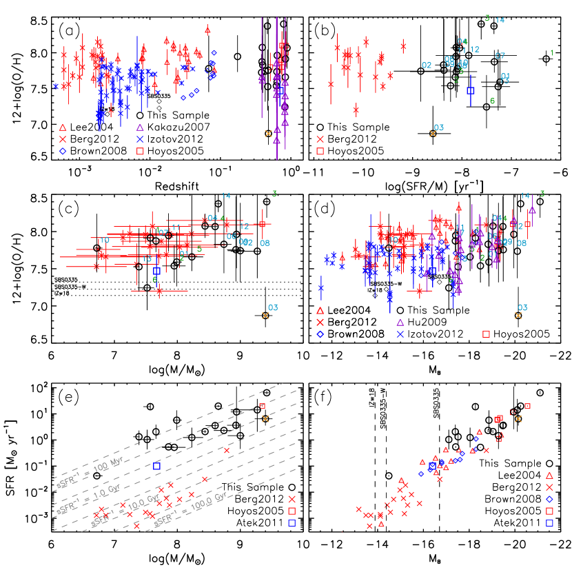
Figure 10.— A comparison of the properties of our [O iii]-A sample (circles) to published direct metallicity studies. The top and middle rows show the gas-phase metallicity vs. (a) redshift; (b) specific SFR; (c) stellar mass; and (d) rest-frame $B$-band absolute magnitude, $M_{B}$. The bottom row shows the SFR vs. (e) stellar mass, and (f) $M_{B}$. Our sample is shown as black circles while the samples of Lee et al. (2004), Hoyos et al. (2005), Brown et al. (2008), Kakazu et al. (2007) and Hu et al. (2009), Atek et al. (2011), Berg et al. (2012) and Izotov et al. (2012a) are shown as red triangles, red squares, blue diamonds, purple triangles, blue squares, red crosses, and blue crosses, respectively. Our only LINER (MMT#03) is denoted by orange crosses. Measurements for I Zw18 and SBS0335 are also overlaid for comparison. We provide 95% C.L. for our metallicity determinations, as well as for published results. Uncertainties on stellar masses, SFRs and other properties are 68% C.L. Where applicable, we apply corrections to SFRs and stellar masses to a consistent Chabrier IMF.

5.5. Dependence on Metallicity with Galaxy Properties

It has been well established that the metal abundance of galaxies correlates with their stellar mass (e.g., Tremonti et al., 2004). The presence of such a correlation and the lack of significant scatter have provided a key constraint in modeling the evolution of galaxies. For example, the shape of the MZR, which shows a turnover in the metallicity at high masses and a steep decline at lower masses, can be explained by a simple model where massive star formation enriches the ISM through stellar feedback. However, such enrichment can drive metals beyond the ISM in low-mass galaxies, and thus lowering their effective metallicity (e.g., Davé et al., 2011).

Studies in the past have been mostly limited toward more massive galaxies ($\gtrsim$10⁹ $M_{\sun}$), and therefore whether the MZR extends toward lower masses or not is unclear with existing limited samples. In Figure 11(a), we illustrate the MZR of AM13, which stacked SDSS spectra to detect [O iii] $\lambda$4363 and determine metallicity using the same method for easier comparison. Here, the MZR is fitted with a logarithmic functional form devised by Moustakas et al. (2011):

$$12\,+\,\log({\rm O/H})=12\,+\,\log({\rm O/H})_{\rm asm}-\log{\left[1+\left(\frac{M_{\rm TO}}{M_{\star}}\right)^{\gamma}\right]},$$ (15)

where 12 + $\log({\rm O/H})$_asm is the asymptotic metallicity at high masses, $M_{\rm TO}$ is the turnover mass, and $\gamma$ controls the slope of the MZR at low masses.

We note that while there are other determinations of the MZR using different strong-line diagnostics that do not require spectra stacking, there are nearly 1 dex differences in metallicity determinations using the same dataset (Kewley & Ellison, 2008). For this reason, we chose to use measurements obtained with the same method. Since AM13 used a different $T_{e}$([O ii])–$T_{e}$([O iii]) relation to determine O⁺/H⁺, we adopt the same relation, $t_{2}=0.7t_{3}+0.1$, for direct comparisons. We note that this difference only raises metallicity on average by 0.05 dex, with $\approx$0.2 dex as the largest correction.

We find that 9 of our 19 galaxies follow the local $T_{e}$-based MZR to within $\pm$2$\sigma$. However, it appears that our entire sample has systematically lower metallicities at all masses. This may be the result of selection effects, since more metal-rich galaxies are less likely to have [O iii] $\lambda$4363 detections.

Recently, some have argued that the MZR is in fact a projection of a more “fundamental” plane between stellar mass, metallicity, and SFR (i.e., $M_{\star}$–$Z$–SFR relation; Lara-López et al., 2010). One such projection, called the “Fundamental Metallicity Relation” (FMR; Mannucci et al., 2010), suggests that galaxies with higher sSFR have lower metallicities compared to those at similar stellar masses. Efforts to describe the FMR have defined a plane in which a tighter correlation exists by considering a combination of stellar mass and SFR:

$$\mu_{\alpha}=\log{\left(\frac{M_{\star}}{M_{\sun}}\right)}-\alpha\log{\left(\frac{{\rm SFR}}{M_{\sun}~{}{\rm yr}^{-1}}\right)},$$ (16)

where $\alpha$ is the coefficient that minimizes the scatter against metallicity. We illustrate the AM13’s determination ($\alpha=0.66$) in Figure 11(b). A comparison against our sample reveals again that roughly half of our galaxies follow the FMR; however, the rest of our metallicities fall below it. Even more interesting, some of our galaxies (i.e., Keck#1, #3, and MMT#14), which followed the MZR are no longer within +2$\sigma$ of the $T_{e}$-based FMR. In these galaxies, the [O iii] $\lambda$4363 detections are robust (S/N = 11.1, 4.6, and 7.6, respectively), and their SFRs are high. If anything, we see a positive or flat correlation between metallicity and sSFR (see Figure 10(b)), contrary to what is expected from the FMR. This might suggest that a $M_{\star}$–$Z$–SFR relation as seen for local galaxies may not hold in low-mass galaxies at $z=0.4$–0.9, and that there is a larger scatter compared to $z\sim 0$.

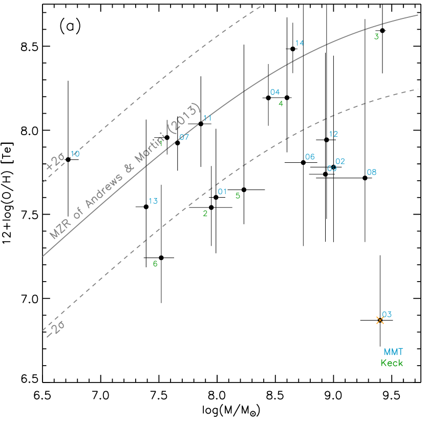
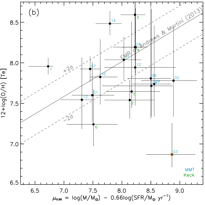
Figure 11.— Comparison of $T_{e}$-based gas metallicity against (a) stellar mass, and (b) a projection of the “FMR” with $\mu=0.66$ for our [O iii]-A sample (black circles). The MZR and FMR of the SDSS derived using the $T_{e}$ method by AM13 are shown in grey with dashed lines indicating $\pm 2\sigma$. Here, the scatter of AM13 is not the true intrinsic scatter from individual galaxies. Rather, it reflects the dispersion for stacked spectra in various $M_{\star}$–SFR bins. This $\sigma$ is likely to be larger than the intrinsic scatter because it is weighted more toward high-SFR outliers (fewer galaxies are available in these bins; B. Andrews 2013, priv. comm.). Metallicity uncertainties are reported at 95% C.L., while 68% C.L. are reported for mass and SFR uncertainties. For direct comparisons, we adopt the same $t_{2}$–$t_{3}$ relation as AM13.

5.6. Number Densities of 12 + $\log({\rm O/H})$ $\lesssim 7.65$ Galaxies

With a statistically meaningful sample of [O iii] $\lambda$4363 detections, we can infer the space density of XMPGs from the largest emission-line sample at intermediate redshifts. As illustrated in Figure 3, we find that our [O iii] $\lambda$4363 sample has rest-frame EWs of EW${}_{0}({\rm H}\alpha)\gtrsim 100$Å and EW${}_{0}([{\rm O}~{}\textsc{iii}])\gtrsim 50$Å. Limiting galaxies to these EWs, we find a number density at $z\sim 0.45$ of $4.5\times 10^{-3}$ Mpc^-3 for H$\alpha$ and $5.1\times 10^{-3}$ Mpc^-3 for [O iii]. Our spectroscopic follow-up sampled a broadly representative range, reaching down to EW₀ = 20Å, and targeted about $\approx$25% of the high-EW galaxies. Among these spectra, 16% and 11% of the H$\alpha$-selected and [O iii]-selected galaxies yielded [O iii] $\lambda$4363 detections, respectively. Extending these statistics to the full high-EW sample, we estimate that the expected number density of galaxies with [O iii] $\lambda$4363 detections at $z=0.3$–0.65 is $7\times 10^{-4}$ Mpc^-3 for H$\alpha$-selected galaxies and $6\times 10^{-4}$ Mpc^-3 for [O iii]-selected galaxies. This corresponds to a surface density of one per 13 arcmin² (H$\alpha$; $z=0.3$–0.5) and one per 8 arcmin² ([O iii]; $z=0.3$–0.65). About one-fifth of these galaxies will have 12 + $\log({\rm O/H})$ $\leq$ 7.65.

The higher rate of XMPGs ($\approx$1%) among star-forming galaxies at high redshift compared to the local universe (recall 1 in 1700 SDSS galaxies are XMPGs) could be a reflection of galaxy evolution. In particular, several lines of evidence have shown that the SFRs and the sSFR’s are an order magnitude higher at $z\gtrsim 1$ than the local universe (e.g., Noeske et al., 2007; Ly et al., 2011b, 2012b; Lee et al., 2012). Future surveys at $z\gtrsim 1$ with JWST and “WFIRST” should find many more XMPGs simply because: (1) the $M_{\star}$–$Z$ relation evolves toward lower metallicity at high redshift (see e.g., Erb et al., 2006); and (2) the epoch of where the SFR density peaked (Hopkins 2004; L07), and where most of the mass assembly occurred (Dickinson et al., 2003; Rudnick et al., 2003), is at $z\sim 1$–3.

Morales-Luis et al. (2011) reported that the number density of XMPGs in the local universe from the SDSS is $\approx 1.3\times 10^{-4}$ Mpc^-3, which is similar to what we find in our study. This comparison would suggest that no evolution is seen in the number density of XMPGs. However, we caution against making such a comparison since the local estimate is highly uncertain due to a statistically small sample that suffers from incompleteness and complex selection functions.

6. CONCLUSIONS

We have conducted an extensive optical spectroscopic survey of nearly 900 ELGs identified in the SDF from NB or IA imaging with Keck/DEIMOS and MMT/Hectospec. Upon inspecting our spectra, we found that we have 20 galaxies where the weak auroral [O iii] $\lambda$4363 line is detected at $\geq$3$\sigma$. These detections allow us to determine the electron temperature of the ionized gas, and directly determine gas-phase metallicity, using the $T_{e}$ method. Excluding our one object which we believe is a LINER, we find that the remaining 19 galaxies are metal-poor with a median 12 + $\log({\rm O/H})$ of 7.75 (0.13 $Z_{\sun}$), and the most metal-rich galaxy having 12 + $\log({\rm O/H})$ = 8.40 (0.5 $Z_{\sun}$). We find that 4 of our galaxies are XMPG (12 + $\log({\rm O/H})$ $\leq$ 7.65).

Our most metal-deficient galaxy with a $\geq$4$\sigma$ detection of [O iii] $\lambda$4363 has an oxygen abundance (12 + $\log({\rm O/H})$ = 7.24${}^{+0.45}_{-0.30}$) that is similar to I Zw 18 and SBS0335. This galaxy lacks an [O ii] detection, which is caused by a high ionization parameter and low metallicity that drive most of the oxygen species to be in a doubly ionized state. In addition, we find that all of our galaxies have high ionization, as measured by [O iii]/H$\beta$, and high electron density ($n_{e}$ = 70–600 cm^-3). While this is not typical for SDSS ELGs, there are rare populations of highly star-forming low-$z$ galaxies found in the SDSS that have high ionization. In addition, these properties are seen for strongly star-forming $z\gtrsim 1$ galaxies. This suggests that XMPGs at $z\sim 0.4$–1 are analogs to high-$z$ star-forming galaxies in terms of their ISM properties.

Our exceptionally deep and complete multi-wavelength dataset in the SDF also allows us to determine other key properties of these galaxies. What we found is that these galaxies are exceptional in several ways.

First, with stellar masses between $5\times 10^{6}$ and $3\times 10^{9}$ $M_{\sun}$ (with a median and average of $3\times 10^{8}$ and $2\times 10^{8}$ $M_{\sun}$, respectively), we find that our galaxies have high specific SFRs, which suggests that these galaxies have assembled their stellar contents in only $\sim$100 Myr. Second, their vigorous star formation is highly concentrated into a small central starburst of high surface density (an average of $\Sigma_{\rm SFR}$ = 0.5 $M_{\sun}$ yr^-1 kpc^-2). Third, they have an excess probability of having nearby companions (within a projected 100 kpc), which we have determined to have strong emission lines at a similar redshift. The presence of nearby companions in two-thirds of our galaxies suggests that galaxy-galaxy interactions may be responsible for the metal deficiency and the observed high sSFRs and high SFR surface densities. In particular, outflowing or inflowing gas can occur through stellar feedback that drives metal-rich gas out of the ISM or gravitational torques that can cause metal-poor gas to lose angular momentum and fall into the center of the galaxies.

Some researchers have proposed that the $M_{\star}$–$Z$ relation must be extended to include a third parameter, the SFR (Lara-López et al., 2010; Mannucci et al., 2010). Since these relations predict lower metallicities for galaxies with unusually high sSFRs, about half of our galaxies are indeed consistent with the FMR. However, there are two inconsistencies that we find. First, our most star-forming galaxies (3 of them) have higher metallicity than what is expected if they followed the FMR. This suggests a flatter or positive correlation between sSFR and $Z$, contrary to an inverse correlation found for the FMR. Second, it appears that our sample has systematically lower metallicity by $\approx$0.2 dex than the FMR. This result is only robust at 2$\sigma$ confidence, and we suspect that selection effects (i.e., required detection of [O iii] $\lambda$4363) may be biasing our sample toward lower metallicity.

The failure of any simple relation to predict O/H can be seen by the large scatter of our metallicities versus stellar mass or sSFR in Figure 11. The large intrinsic scatter overwhelms any other trends with metallicity which might be present. For example, our sample contains 19 galaxies with redshifts ranging from $z$=0.38–0.88 (excluding the lowest redshift galaxy), a range of look-back times from 4 to 7 Gyr. This period of cosmic history is known to span a great deal of evolution in many properties of the overall galaxy population as a whole. Nonetheless our galaxy sample shows no trend of metallicity with redshift. Across all of these redshifts, we find galaxies with half solar abundances mixed in with very metal-poor galaxies. We believe that this large cosmic scatter of abundances is larger than our measurement uncertainties, and is genuine.

Table 5Emission-line Ratios, Electron Temperatures, and Gas-Phase Metallicities

ID	$\log{\left(\frac{[{\rm O}~{}\textsc{iii}]}{[{\rm O}~{}\textsc{iii}]\ \lambda 4363}\right)}$		$\log{(T_{e}/{\rm K})}$		$\log{\left(\frac{[{\rm O}~{}\textsc{ii}]}{{\rm H}\beta}\right)}$		$\log{\left(\frac{[{\rm O}~{}\textsc{iii}]}{{\rm H}\beta}\right)}$	$\log{\left(\frac{{\rm O}^{+}}{{\rm H}^{+}}\right)}$		$\log{\left(\frac{{\rm O}^{++}}{{\rm H}^{+}}\right)}$	$12+\log{\left(\frac{{\rm O}}{{\rm H}}\right)}$
(1)	(2)	(3)	(4)	(5)	(6)	(7)	(8)	(9)	(10)	(11)	(12)	(13)
MMT#01	1.52${}^{+0.24}_{-0.17}$	1.46${}^{+0.23}_{-0.21}$	4.32${}^{+0.12}_{-0.13}$	4.37${}^{+0.16}_{-0.15}$	+0.06${}^{+0.09}_{-0.08}$	+0.18${}^{+0.20}_{-0.17}$	0.89${}^{+0.08}_{-0.07}$	-4.99${}^{+0.50}_{-0.34}$	-4.84${}^{+0.54}_{-0.39}$	-4.61${}^{+0.29}_{-0.30}$	7.60${}^{+0.37}_{-0.26}$	7.59${}^{+0.40}_{-0.33}$
MMT#02	1.61${}^{+0.40}_{-0.24}$	1.55${}^{+0.39}_{-0.28}$	4.27${}^{+0.16}_{-0.18}$	4.31${}^{+0.22}_{-0.21}$	+0.50${}^{+0.04}_{-0.04}$	+0.62${}^{+0.29}_{-0.17}$	0.64${}^{+0.04}_{-0.04}$	-4.54${}^{+0.70}_{-0.44}$	-4.43${}^{+0.74}_{-0.49}$	-4.74${}^{+0.47}_{-0.38}$	7.71${}^{+0.60}_{-0.42}$	7.74${}^{+0.64}_{-0.43}$
MMT#03	1.17${}^{+0.24}_{-0.21}$	1.09${}^{+0.29}_{-0.27}$	4.60${}^{+0.10}_{-0.22}$	4.65${}^{+0.09}_{-0.20}$	+0.56${}^{+0.05}_{-0.04}$	+0.74${}^{+0.21}_{-0.20}$	0.34${}^{+0.05}_{-0.05}$	…	…	…	…	…
MMT#04	1.95${}^{+0.14}_{-0.12}$	1.95${}^{+0.14}_{-0.13}$	4.11${}^{+0.05}_{-0.05}$	4.11${}^{+0.05}_{-0.05}$	+0.36${}^{+0.01}_{-0.01}$	+0.36${}^{+0.03}_{-0.01}$	0.77${}^{+0.01}_{-0.01}$	-4.37${}^{+0.20}_{-0.18}$	-4.37${}^{+0.21}_{-0.17}$	-4.12${}^{+0.15}_{-0.15}$	8.07${}^{+0.17}_{-0.15}$	8.07${}^{+0.17}_{-0.16}$
MMT#05	1.66${}^{+0.19}_{-0.17}$	1.66${}^{+0.19}_{-0.16}$	4.24${}^{+0.08}_{-0.12}$	4.24${}^{+0.10}_{-0.12}$	-0.27${}^{+0.09}_{-0.10}$	-0.27${}^{+0.15}_{-0.10}$	0.92${}^{+0.03}_{-0.03}$	-5.27${}^{+0.36}_{-0.27}$	-5.27${}^{+0.38}_{-0.25}$	-4.32${}^{+0.22}_{-0.24}$	7.72${}^{+0.26}_{-0.20}$	7.72${}^{+0.26}_{-0.24}$
MMT#06	1.42${}^{+0.41}_{-0.25}$	1.32${}^{+0.41}_{-0.25}$	4.32${}^{+0.22}_{-0.33}$	4.40${}^{+0.19}_{-0.38}$	+0.54${}^{+0.06}_{-0.05}$	+0.73${}^{+0.07}_{-0.06}$	0.54${}^{+0.05}_{-0.05}$	-4.52${}^{+0.89}_{-0.46}$	-4.24${}^{+1.16}_{-0.51}$	-5.01${}^{+0.72}_{-0.27}$	7.65${}^{+0.81}_{-0.46}$	7.83${}^{+1.11}_{-0.39}$
MMT#07	1.84${}^{+0.11}_{-0.08}$	1.78${}^{+0.12}_{-0.13}$	4.15${}^{+0.04}_{-0.05}$	4.18${}^{+0.07}_{-0.06}$	-0.02${}^{+0.01}_{-0.02}$	+0.10${}^{+0.17}_{-0.13}$	0.87${}^{+0.01}_{-0.01}$	-4.87${}^{+0.17}_{-0.13}$	-4.81${}^{+0.19}_{-0.15}$	-4.23${}^{+0.16}_{-0.18}$	7.92${}^{+0.13}_{-0.12}$	7.87${}^{+0.16}_{-0.15}$
MMT#08	1.37${}^{+0.31}_{-0.24}$	1.26${}^{+0.41}_{-0.33}$	4.31${}^{+0.22}_{-0.35}$	4.40${}^{+0.20}_{-0.45}$	+0.40${}^{+0.09}_{-0.10}$	+0.61${}^{+0.36}_{-0.27}$	0.58${}^{+0.10}_{-0.10}$	-4.65${}^{+0.79}_{-0.49}$	-4.36${}^{+1.08}_{-0.43}$	-4.97${}^{+0.61}_{-0.29}$	7.58${}^{+0.70}_{-0.46}$	7.74${}^{+0.99}_{-0.36}$
MMT#09	1.43${}^{+0.29}_{-0.22}$	1.34${}^{+0.29}_{-0.26}$	4.32${}^{+0.19}_{-0.28}$	4.40${}^{+0.20}_{-0.26}$	+0.39${}^{+0.10}_{-0.09}$	+0.58${}^{+0.13}_{-0.12}$	0.76${}^{+0.09}_{-0.09}$	-4.66${}^{+0.64}_{-0.51}$	-4.39${}^{+0.79}_{-0.47}$	-4.79${}^{+0.42}_{-0.33}$	7.65${}^{+0.55}_{-0.42}$	7.76${}^{+0.72}_{-0.43}$
MMT#10	1.75${}^{+0.33}_{-0.21}$	1.72${}^{+0.33}_{-0.21}$	4.20${}^{+0.10}_{-0.14}$	4.21${}^{+0.11}_{-0.15}$	+0.09${}^{+0.04}_{-0.04}$	+0.14${}^{+0.04}_{-0.06}$	0.82${}^{+0.02}_{-0.02}$	-4.85${}^{+0.51}_{-0.32}$	-4.82${}^{+0.47}_{-0.32}$	-4.35${}^{+0.38}_{-0.30}$	7.80${}^{+0.41}_{-0.25}$	7.78${}^{+0.46}_{-0.33}$
MMT#11	1.85${}^{+0.21}_{-0.15}$	1.80${}^{+0.21}_{-0.16}$	4.15${}^{+0.08}_{-0.08}$	4.17${}^{+0.08}_{-0.09}$	+0.29${}^{+0.03}_{-0.03}$	+0.39${}^{+0.04}_{-0.03}$	0.82${}^{+0.02}_{-0.02}$	-4.55${}^{+0.29}_{-0.27}$	-4.50${}^{+0.31}_{-0.27}$	-4.24${}^{+0.27}_{-0.20}$	7.97${}^{+0.26}_{-0.21}$	7.95${}^{+0.30}_{-0.22}$
MMT#12	1.45${}^{+0.42}_{-0.24}$	1.32${}^{+0.54}_{-0.44}$	4.29${}^{+0.21}_{-0.29}$	4.40${}^{+0.24}_{-0.46}$	+0.58${}^{+0.14}_{-0.12}$	+0.84${}^{+0.60}_{-0.36}$	0.81${}^{+0.13}_{-0.12}$	-4.46${}^{+0.90}_{-0.46}$	-4.13${}^{+1.24}_{-0.42}$	-4.74${}^{+0.80}_{-0.42}$	7.80${}^{+0.78}_{-0.43}$	7.96${}^{+1.14}_{-0.46}$
MMT#13	1.57${}^{+0.37}_{-0.20}$	1.52${}^{+0.31}_{-0.27}$	4.30${}^{+0.15}_{-0.20}$	4.32${}^{+0.19}_{-0.23}$	-0.02${}^{+0.08}_{-0.08}$	+0.07${}^{+0.23}_{-0.16}$	0.78${}^{+0.03}_{-0.04}$	-5.06${}^{+0.57}_{-0.46}$	-4.98${}^{+0.69}_{-0.45}$	-4.64${}^{+0.43}_{-0.34}$	7.54${}^{+0.52}_{-0.30}$	7.53${}^{+0.52}_{-0.33}$
MMT#14	2.22${}^{+0.12}_{-0.10}$	2.21${}^{+0.15}_{-0.11}$	4.01${}^{+0.03}_{-0.04}$	4.01${}^{+0.04}_{-0.04}$	+0.25${}^{+0.01}_{-0.01}$	+0.27${}^{+0.03}_{-0.02}$	0.79${}^{+0.01}_{-0.01}$	-4.11${}^{+0.20}_{-0.15}$	-4.10${}^{+0.17}_{-0.13}$	-3.80${}^{+0.16}_{-0.10}$	8.38${}^{+0.16}_{-0.12}$	8.37${}^{+0.17}_{-0.11}$
Keck#1	1.92${}^{+0.08}_{-0.08}$	1.81${}^{+0.09}_{-0.09}$	4.12${}^{+0.03}_{-0.03}$	4.17${}^{+0.04}_{-0.04}$	-0.22${}^{+0.03}_{-0.03}$	-0.02${}^{+0.06}_{-0.08}$	0.90${}^{+0.01}_{-0.01}$	-4.99${}^{+0.13}_{-0.12}$	-4.89${}^{+0.14}_{-0.13}$	-4.16${}^{+0.10}_{-0.09}$	8.01${}^{+0.09}_{-0.08}$	7.91${}^{+0.12}_{-0.10}$
Keck#2	1.44${}^{+0.15}_{-0.13}$	1.44${}^{+0.15}_{-0.13}$	4.38${}^{+0.09}_{-0.11}$	4.38${}^{+0.09}_{-0.11}$	+0.14${}^{+0.04}_{-0.04}$	+0.14${}^{+0.04}_{-0.04}$	0.84${}^{+0.02}_{-0.02}$	-4.86${}^{+0.36}_{-0.30}$	-4.86${}^{+0.36}_{-0.30}$	-4.68${}^{+0.20}_{-0.19}$	7.54${}^{+0.27}_{-0.22}$	7.54${}^{+0.27}_{-0.22}$
Keck#3	2.30${}^{+0.21}_{-0.18}$	2.14${}^{+0.22}_{-0.16}$	3.98${}^{+0.05}_{-0.06}$	4.03${}^{+0.06}_{-0.08}$	+0.35${}^{+0.01}_{-0.01}$	+0.66${}^{+0.04}_{-0.04}$	0.68${}^{+0.01}_{-0.01}$	-3.90${}^{+0.33}_{-0.23}$	-3.82${}^{+0.28}_{-0.23}$	-4.00${}^{+0.26}_{-0.18}$	8.44${}^{+0.29}_{-0.22}$	8.40${}^{+0.31}_{-0.22}$
Keck#4	2.02${}^{+0.29}_{-0.23}$	2.02${}^{+0.29}_{-0.23}$	4.08${}^{+0.09}_{-0.11}$	4.08${}^{+0.09}_{-0.11}$	+0.27${}^{+0.02}_{-0.02}$	+0.27${}^{+0.02}_{-0.02}$	0.68${}^{+0.01}_{-0.01}$	-4.37${}^{+0.46}_{-0.34}$	-4.37${}^{+0.46}_{-0.34}$	-4.13${}^{+0.36}_{-0.26}$	8.07${}^{+0.41}_{-0.29}$	8.07${}^{+0.41}_{-0.29}$
Keck#5	1.16${}^{+0.35}_{-0.24}$	1.10${}^{+0.37}_{-0.25}$	4.36${}^{+0.16}_{-0.77}$	4.40${}^{+0.14}_{-0.76}$	+0.24${}^{+0.05}_{-0.05}$	+0.36${}^{+0.22}_{-0.16}$	0.88${}^{+0.03}_{-0.04}$	-4.79${}^{+1.04}_{-0.28}$	-4.61${}^{+1.10}_{-0.33}$	-4.67${}^{+0.60}_{-0.15}$	7.61${}^{+0.86}_{-0.26}$	7.66${}^{+0.90}_{-0.19}$
Keck#6	1.41${}^{+0.24}_{-0.18}$	1.35${}^{+0.32}_{-0.23}$	4.35${}^{+0.16}_{-0.24}$	4.40${}^{+0.17}_{-0.27}$	-1.14${}^{+0.51}_{-0.83}$	-1.02${}^{+0.59}_{-0.94}$	0.77${}^{+0.03}_{-0.03}$	-6.18${}^{+0.99}_{-1.02}$	-5.99${}^{+1.06}_{-1.03}$	-4.78${}^{+0.39}_{-0.29}$	7.32${}^{+0.47}_{-0.25}$	7.24${}^{+0.45}_{-0.30}$

Note. — Columns (3), (5), (7), (10), and (13) include dust attenution corrections (see Section 4.1). Errors are reported at the 95% C.L.

Table 6Luminosities, Stellar Properties, and Star Formation Rates

ID	$M_{B}$	$\log{\left[\frac{{\rm SFR}({\rm H}\alpha)}{M_{\sun}/{\rm yr}}\right]}$		$\log{\left[\frac{{\rm SFR}({\rm H}\beta)}{M_{\sun}/{\rm yr}}\right]}$		$\log{({\rm M}_{\star}/M_{\sun})}$		$\log{(t_{\rm age}/{\rm yr})}$		$A_{V}$
		Obs.	De-red.	Obs.	De-red.	0.2$Z_{\sun}$	$Z_{\sun}$	0.2$Z_{\sun}$	$Z_{\sun}$	0.2$Z_{\sun}$	$Z_{\sun}$
(1)	(2)	(3)	(4)	(5)	(6)	(7)	(8)	(9)	(10)	(11)	(12)
MMT#01	–18.67	…	…	+0.32	+0.76${}^{+0.38}_{-0.38}$	7.99${}^{+0.08}_{-0.06}$	8.23${}^{+0.08}_{-0.33}$	7.40${}^{+0.17}_{-0.29}$	8.10${}^{+0.24}_{-0.98}$	0.6${}^{+0.1}_{-0.1}$	0.3${}^{+0.5}_{-0.2}$
MMT#02	–19.28	…	…	–0.29	+0.17${}^{+0.37}_{-0.41}$	9.00${}^{+0.07}_{-0.20}$	9.23${}^{+0.01}_{-0.09}$	8.60${}^{+0.22}_{-0.93}$	9.00${}^{+0.12}_{-0.29}$	0.9${}^{+0.3}_{-0.1}$	0.7${}^{+0.2}_{-0.1}$
MMT#03	–20.15	+0.35	+0.81${}^{+0.35}_{-0.32}$	…	…	9.40${}^{+0.11}_{-0.17}$	9.59${}^{+0.09}_{-0.04}$	8.50${}^{+0.30}_{-0.80}$	8.90${}^{+0.24}_{-0.20}$	1.1${}^{+0.2}_{-0.2}$	0.9${}^{+0.1}_{-0.1}$
MMT#04	–19.07	+0.32	+0.32${}^{+0.06}_{-0.06}$	…	…	8.44${}^{+0.02}_{-0.05}$	8.60${}^{+0.08}_{-0.11}$	7.50${}^{+0.35}_{-0.10}$	8.20${}^{+0.32}_{-0.50}$	0.7${}^{+0.2}_{-0.3}$	0.6${}^{+0.1}_{-0.3}$
MMT#05	…	…	…	–0.34	–0.34${}^{+0.39}_{-0.38}$	…	…	…	…	…	…
MMT#06	–18.83	–0.15	+0.37${}^{+0.05}_{-0.05}$	…	…	8.74${}^{+0.12}_{-0.16}$	9.01${}^{+0.02}_{-0.09}$	8.40${}^{+0.40}_{-0.71}$	9.00${}^{+0.12}_{-0.24}$	0.9${}^{+0.2}_{-0.2}$	0.6${}^{+0.1}_{-0.1}$
MMT#07	–17.61	–0.00	+0.32${}^{+0.27}_{-0.27}$	…	…	7.66${}^{+0.00}_{-0.00}$	7.62${}^{+0.00}_{-0.00}$	7.40${}^{+0.00}_{-0.00}$	7.40${}^{+0.00}_{-0.00}$	0.5${}^{+0.0}_{-0.0}$	0.4${}^{+0.0}_{-0.0}$
MMT#08	–20.13	…	…	+0.38	+1.15${}^{+0.79}_{-0.84}$	9.27${}^{+0.06}_{-0.42}$	9.35${}^{+0.11}_{-0.00}$	8.20${}^{+0.29}_{-1.20}$	8.30${}^{+0.42}_{-0.14}$	1.2${}^{+0.4}_{-0.4}$	0.8${}^{+0.3}_{-0.0}$
MMT#09	–19.50	+0.06	+0.56${}^{+0.12}_{-0.13}$	…	…	8.93${}^{+0.08}_{-0.14}$	9.14${}^{+0.09}_{-0.02}$	8.50${}^{+0.34}_{-0.80}$	8.90${}^{+0.29}_{-0.12}$	0.7${}^{+0.1}_{-0.2}$	0.5${}^{+0.1}_{-0.2}$
MMT#10	–14.57	–1.52	–1.37${}^{+0.02}_{-0.03}$	…	…	6.72${}^{+0.09}_{-0.03}$	7.01${}^{+0.33}_{-0.04}$	7.10${}^{+0.31}_{-0.10}$	7.80${}^{+1.28}_{-0.04}$	1.6${}^{+0.1}_{-0.2}$	0.7${}^{+0.2}_{-0.3}$
MMT#11	–17.28	–0.52	–0.26${}^{+0.04}_{-0.03}$	…	…	7.86${}^{+0.09}_{-0.11}$	8.09${}^{+0.18}_{-0.08}$	7.80${}^{+0.39}_{-0.52}$	8.50${}^{+0.54}_{-0.44}$	0.9${}^{+0.3}_{-0.4}$	0.6${}^{+0.2}_{-0.3}$
MMT#12	–19.92	…	…	+0.14	+1.08${}^{+1.33}_{-0.84}$	8.94${}^{+0.08}_{-0.09}$	9.11${}^{+0.09}_{-0.09}$	8.10${}^{+0.42}_{-0.44}$	8.60${}^{+0.22}_{-0.39}$	0.6${}^{+0.3}_{-0.4}$	0.5${}^{+0.1}_{-0.2}$
MMT#13	–17.52	–0.11	+0.12${}^{+0.35}_{-0.31}$	…	…	7.39${}^{+0.01}_{-0.09}$	7.28${}^{+0.32}_{-0.09}$	7.30${}^{+0.10}_{-0.10}$	7.10${}^{+0.96}_{-0.10}$	0.3${}^{+0.1}_{-0.0}$	0.5${}^{+0.1}_{-0.5}$
MMT#14	–20.25	+1.26	+1.30${}^{+0.04}_{-0.04}$	…	…	8.65${}^{+0.04}_{-0.06}$	8.49${}^{+0.01}_{-0.03}$	7.30${}^{+0.12}_{-0.08}$	7.10${}^{+0.05}_{-0.10}$	0.6${}^{+0.0}_{-0.1}$	0.7${}^{+0.1}_{-0.1}$
Keck#1	–18.08	…	…	+0.52	+1.28${}^{+0.14}_{-0.13}$	7.57${}^{+0.00}_{-0.11}$	7.39${}^{+0.00}_{-0.07}$	7.30${}^{+0.07}_{-0.08}$	7.00${}^{+0.04}_{-0.00}$	0.0${}^{+0.1}_{-0.0}$	0.2${}^{+0.0}_{-0.1}$
Keck#2	–18.38	…	…	–0.29	–0.29	7.95${}^{+0.18}_{-0.19}$	8.29${}^{+0.05}_{-0.14}$	7.30${}^{+0.67}_{-0.30}$	8.30${}^{+0.21}_{-0.60}$	0.9${}^{+0.1}_{-0.3}$	0.4${}^{+0.2}_{-0.4}$
Keck#3	–21.12	…	…	+0.67	+1.81${}^{+0.08}_{-0.07}$	9.42${}^{+0.03}_{-0.06}$	9.46${}^{+0.01}_{-0.05}$	7.50${}^{+0.41}_{-0.17}$	7.70${}^{+0.12}_{-0.06}$	1.0${}^{+0.3}_{-0.8}$	0.6${}^{+0.0}_{-0.3}$
Keck#4	–19.45	…	…	+0.55	+0.55${}^{+0.12}_{-0.12}$	8.60${}^{+0.04}_{-0.15}$	8.47${}^{+0.05}_{-0.09}$	7.30${}^{+0.28}_{-0.23}$	7.10${}^{+0.21}_{-0.10}$	1.0${}^{+0.1}_{-0.1}$	1.2${}^{+0.1}_{-0.1}$
Keck#5	–18.05	…	…	–0.35	+0.09${}^{+0.38}_{-0.38}$	8.23${}^{+0.18}_{-0.14}$	8.47${}^{+0.18}_{-0.12}$	8.70${}^{+0.44}_{-0.64}$	9.10${}^{+0.20}_{-0.38}$	0.2${}^{+0.4}_{-0.2}$	0.0${}^{+0.2}_{-0.0}$
Keck#6	–17.16	…	…	–0.42	+0.02${}^{+0.38}_{-0.38}$	7.52${}^{+0.11}_{-0.15}$	7.45${}^{+0.06}_{-0.07}$	7.30${}^{+0.18}_{-0.30}$	7.00${}^{+0.10}_{-0.00}$	1.1${}^{+0.2}_{-0.2}$	1.3${}^{+0.1}_{-0.1}$

Note. — All values assume a Chabrier IMF, and where applicable, dust attenuation follows C00 formalism. 68% confidence measurement uncertainties are reported.

Table 7Spectral Energy Distributions

ID	FUV	NUV	$U$	$B$	$V$	IA598	$R_{\rm C}$	IA679	$i$′	$z_{b}$	$z$′	$z_{r}$	$J$	$H$	$K$
(1)	(2)	(3)	(4)	(5)	(6)	(7)	(8)	(9)	(10)	(11)	(12)	(13)	(14)	(15)	(16)
MMT#01	0.26$\pm$0.04	0.93$\pm$0.03	0.97$\pm$0.03	0.89	1.00	1.37$\pm$0.03	1.41	1.24$\pm$0.02	2.36	1.14	1.16	1.06$\pm$0.09	1.00$\pm$0.47	2.75$\pm$1.89	1.44$\pm$0.26
…	…	…	…	…	…	-0.43	-0.28	-0.11	-1.09	…	-0.04	…	…	…	…
MMT#02	0.62$\pm$0.05	1.46$\pm$0.04	1.86$\pm$0.03	2.01	3.57	4.51$\pm$0.03	4.97	5.01$\pm$0.02	5.61	5.93	6.59	7.17$\pm$0.10	9.46$\pm$0.66	10.13$\pm$1.63	…
…	…	…	…	…	-0.22	…	-0.18	-0.09	-0.37	…	-0.24	-0.08	…	…	…
MMT#03	0.70$\pm$0.05	1.96$\pm$0.04	2.88$\pm$0.03	3.07	5.24	7.44$\pm$0.03	8.31	8.78$\pm$0.02	9.51	10.86	11.35	15.18$\pm$0.10	17.15$\pm$0.72	22.32$\pm$1.84	…
…	…	…	…	…	-0.25	-0.05	-0.05	…	-0.24	…	-0.67	-3.16	…	…	…
MMT#04	1.73$\pm$0.07	2.86$\pm$0.05	3.28$\pm$0.03	3.04	4.76	4.98$\pm$0.03	7.03	8.38$\pm$0.02	5.97	7.53	7.00	5.82$\pm$0.10	9.16$\pm$0.59	10.11$\pm$1.23	7.24$\pm$0.28
…	…	…	…	…	-0.69	-0.43	-1.97	-3.41	-1.09	-2.39	-1.82	-0.01	…	…	…
MMT#06	0.64$\pm$0.05	1.40$\pm$0.06	1.64$\pm$0.03	1.74	3.15	3.69$\pm$0.03	4.28	4.52$\pm$0.02	4.51	5.57	5.60	5.41$\pm$0.10	7.45$\pm$0.71	10.57$\pm$1.82	7.19$\pm$0.28
…	…	…	…	…	-0.23	-0.17	-0.37	-0.51	-0.22	-0.66	-0.57	…	…	…	…
MMT#07	0.63$\pm$0.04	1.11$\pm$0.04	1.26$\pm$0.03	1.19	1.70	1.69$\pm$0.03	3.62	5.69$\pm$0.02	2.44	3.28	2.78	1.64$\pm$0.09	3.17$\pm$0.75	4.52$\pm$1.17	1.94$\pm$0.27
…	…	…	…	…	-0.42	-0.48	-2.29	-4.86	-1.13	-1.79	-1.31	…	…	…	…
MMT#08	0.17$\pm$0.03	1.11$\pm$0.04	1.71$\pm$0.03	1.87	2.46	3.81$\pm$0.03	4.34	4.66$\pm$0.02	5.57	5.43	5.40	6.01$\pm$0.10	6.99$\pm$0.69	10.37$\pm$1.69	…
…	…	…	…	…	-0.01	-1.07	-0.41	-0.08	-0.80	…	-0.02	…	…	…	…
MMT#09	0.85$\pm$0.05	2.12$\pm$0.06	2.23$\pm$0.03	2.03	3.29	4.43$\pm$0.03	4.73	4.93$\pm$0.02	5.50	5.47	5.76	7.49$\pm$0.10	8.99$\pm$0.67	10.56$\pm$1.69	…
…	…	…	…	…	-0.22	-0.05	-0.14	…	-0.62	…	-0.36	-1.71	…	…	…
MMT#10	0.82$\pm$0.06	1.15$\pm$0.03	1.89$\pm$0.03	2.68	4.98	3.57$\pm$0.03	4.75	4.22$\pm$0.02	4.84	4.56	4.66	5.33$\pm$0.10	5.64$\pm$0.69	9.85$\pm$1.49	3.38$\pm$0.28
…	…	…	-0.03	-0.27	-1.43	…	-0.65	-0.18	-0.66	…	…	…	…	…	…
MMT#11	1.93$\pm$0.09	2.77$\pm$0.09	3.37$\pm$0.03	4.05	6.99	9.59$\pm$0.03	6.18	6.16$\pm$0.02	7.41	6.95	6.85	6.90$\pm$0.10	10.02$\pm$0.70	9.74$\pm$1.61	7.46$\pm$0.28
…	…	…	…	-0.44	-1.73	-3.73	-0.29	…	-1.11	…	…	…	…	…	…
MMT#12	0.34$\pm$0.04	1.82$\pm$0.08	2.01$\pm$0.03	1.91	2.26	3.15$\pm$0.03	3.60	3.80$\pm$0.02	4.41	4.10	4.02	4.20$\pm$0.10	4.16$\pm$0.74	4.22$\pm$1.63	…
…	…	…	…	…	…	-0.90	-0.34	-0.04	-0.62	…	-0.02	…	…	…	…
MMT#13	0.51$\pm$0.04	0.84$\pm$0.06	0.66$\pm$0.03	0.66	0.85	0.89$\pm$0.03	0.88	0.77$\pm$0.02	1.26	0.60	0.94	2.06$\pm$0.10	0.79$\pm$0.66	$\leq$1.62	1.21$\pm$0.26
…	…	…	…	…	-0.09	-0.06	-0.09	…	-0.62	…	-0.33	-1.50	…	…	…
MMT#14	3.81$\pm$0.11	7.68$\pm$0.15	9.16$\pm$0.03	8.64	11.57	10.59$\pm$0.03	10.76	9.69$\pm$0.02	15.73	10.03	13.16	27.56$\pm$0.10	12.44$\pm$0.76	12.66$\pm$1.82	13.34$\pm$0.29
…	…	…	…	…	-1.54	-0.58	-0.82	…	…	…	-4.84	-20.59	…	…	-0.02
Keck#1	$\leq$0.03	0.93$\pm$0.05	0.55$\pm$0.03	0.51	0.54	0.55$\pm$0.03	0.65	0.79$\pm$0.02	0.66	1.85	1.65	0.31$\pm$0.09	1.17$\pm$0.74	$\leq$1.62	…
…	…	…	…	…	…	…	-0.07	-0.21	-0.14	-1.60	-1.39	-0.02	-0.56	…	…
Keck#2	0.15$\pm$0.03	0.62$\pm$0.03	0.59$\pm$0.03	0.61	0.69	0.91$\pm$0.03	0.99	0.95$\pm$0.02	1.27	0.94	0.96	0.88$\pm$0.09	0.84$\pm$0.66	2.19$\pm$1.48	1.21$\pm$0.26
…	…	…	…	…	…	-0.14	-0.07	-0.03	-0.26	…	…	…	…	…	…
Keck#3	$\leq$0.03	3.70$\pm$0.13	4.20$\pm$0.03	3.81	4.46	4.77$\pm$0.03	5.91	7.65$\pm$0.02	7.54	10.23	9.36	8.38$\pm$0.10	13.20$\pm$0.71	15.65$\pm$1.83	…
…	…	…	…	…	…	…	-0.40	-1.38	-0.13	-2.55	-1.76	…	-1.09	…	…
Keck#4	$\leq$0.03	0.55$\pm$0.03	0.78$\pm$0.03	0.80	0.98	1.01$\pm$0.03	1.25	1.14$\pm$0.02	1.51	1.56	2.25	1.74$\pm$0.09	2.57$\pm$0.62	1.84$\pm$0.95	2.12$\pm$0.27
…	…	…	…	…	…	…	-0.14	-0.03	-0.33	-0.22	-0.62	-0.20	-0.63	…	…
Keck#5	$\leq$0.03	0.28$\pm$0.02	0.20$\pm$0.03	0.21	0.24	0.18$\pm$0.03	0.30	0.36$\pm$0.02	0.40	0.68	0.63	0.25$\pm$0.08	1.05$\pm$0.58	$\leq$1.62	0.54$\pm$0.24
…	…	…	…	…	…	…	-0.03	-0.08	-0.05	-0.23	-0.19	…	-0.08	…	…
Keck#6	$\leq$0.03	$\leq$0.03	0.03$\pm$0.07	0.10	0.11	0.08$\pm$0.02	0.15	0.13$\pm$0.01	0.13	0.50	0.37	$\leq$0.10	$\leq$0.61	$\leq$1.62	…
…	…	…	…	…	…	…	…	…	-0.03	-0.19	-0.14	…	-0.07	…	…

Note. — All fluxes are provided in units of $\mu$Jy. Flux uncertainties for $B$, $V$, $R_{\rm C}$, and $i$′ are 0.01 $\mu$Jy, and 0.04 and 0.03 for $z_{b}$ and $z$′, respectively. All uncertainties are reported at the 68% C.L.

Appendix A Accurate Flux Calibration of MMT/Hectospec and Keck/DEIMOS Spectra

Since the spectroscopic data were obtained from two different instruments, MMT/Hectospec and Keck/DEIMOS, using different observational configurations (fibers versus slits) and in various observational conditions (seeing: 0$\farcs$5–1$\farcs$5), the flux calibration of our data is problematic. To better unify the spectroscopic data, we use the following approach.

First, spectro-photometric standard stars were observed. These observations were generally obtained on the same night; however, in some cases, these calibration data were taken a few days apart. Reducing the calibration data in identical or similar ways to our science spectra, we determine the sensitivity function(s) using standard iraf processing techniques. We then apply these sensitivity functions to our data to yield “first-pass” flux-calibrated spectroscopic products.

Second, we examine the reliability of our flux calibration for each slit mask or fiber configuration by comparing them to broad-band photometric data. Here we only consider the brightest galaxies such that the continuum is well-detected. For the MMT and DEIMOS data, we restrict the calibration sample to $R_{\rm C}\leq 22.0$ mag and $i\arcmin\leq 23.0$ mag, respectively. This typically has 10 galaxies per set-up. To avoid the effects of OH skylines, we generate smoothed spectra where a boxcar median is used. From there we convolved our smoothed spectra against the filter responses and determine fluxes. These fluxes are compared against the photometric data to examine slit/fiber losses and if any second-order wavelength-dependent corrections are needed. In most cases, the comparison against photometric data only showed a systematic offset due to slit/fiber losses. This comparison showed that the rms is typically between 10%–20%.

Next, to ensure that the flux calibration is reliable, we use our measurements of nebular emission lines from NB imaging data to compare against the spectroscopic measurements. The NB fluxes are derived from Equation (6) but differs for each NB filter. We use the spectroscopic redshift to correct the NB flux for when the emission line falls in the filter’s wing. This comparison is illustrated in Figure 12. For 116 NB816 emitters with MMT spectroscopy, we find excellent agreement with a small offset (–0.036 dex) and an rms of 0.155 dex. Similar results are also seen for 108 NB704 emitters. We note that these calibration results are consistent with those obtained by the Hectospec instrument team (Fabricant et al., 2008). In addition, the DEIMOS fluxes also show great agreement for 58 NB921 emitters. Similar results are also seen for 9 NB704, 39 NB816, and 8 NB973 emitters. This consistent agreement at multiple wavelengths supports our wavelength-dependent flux calibration. Note that in our second step we only use broad-band data, so this comparison against NB data is an independent test.

Finally, a second test that we conducted is to examine the emission-line flux determinations for the same galaxies in different observing conditions. This was only feasible with MMT because of the wide field-of-view to target multiple galaxies simultaneously. In total, we have 28 galaxies with two spectra. We illustrate in Figure 13 the determination of fluxes for various emission lines that span rest-frame wavelengths of 3700Å–6730Å and observed wavelengths of 4000Å–8300Å. We find that between different MMT setups, the same emission-line fluxes are obtained with an rms of 0.15–0.20 dex across a wide spectral range, which further supports our approach for accurate flux calibration.

We note that the effects of differential refraction are mitigated for the MMT spectra, as an atmospheric dispersion compensator (ADC) is used and is known to eliminate issues affecting the flux calibration of the spectra (Fabricant et al., 2008). DEIMOS, however, does not have an ADC. The wavelength-dependent effects of differential refraction are seen in some of our DEIMOS observations when comparisons are made against broad-band data. Since our data are calibrated against broad-band photometry, as discussed above, these issues are resolved (to first order).

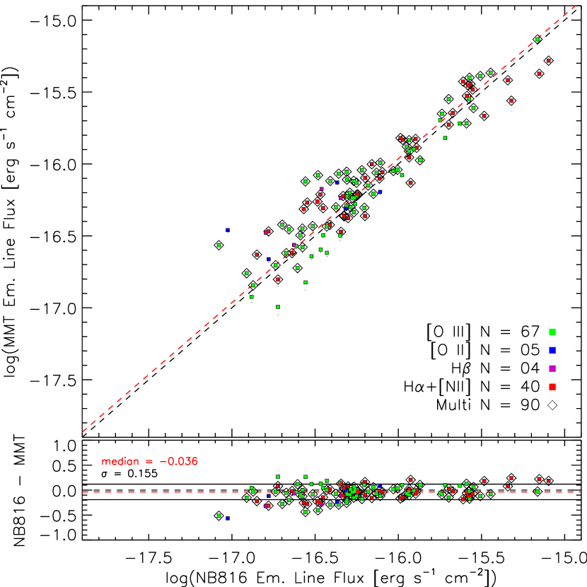
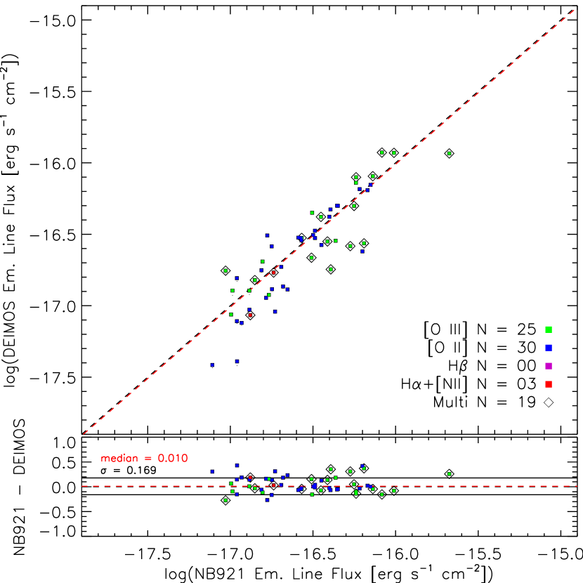
Figure 12.— Comparison between spectroscopic flux measurements against NB fluxes. The left (right) panel shows the MMT (DEIMOS) flux measurements for NB816 (NB921) emitters. Measurements for H$\alpha$+[N ii], [O iii], H$\beta$, and [O ii] are shown as red, green, purple, and blue, respectively. Diamonds denote those measurements where more than one emission line enters the NB filter (e.g., H$\alpha$ and [N ii], or [O iii] $\lambda$4959,5007). These figures demonstrate that the flux calibration is precise and accurate for both MMT and DEIMOS. Other NB emitters have been inspected and similar results have been found.

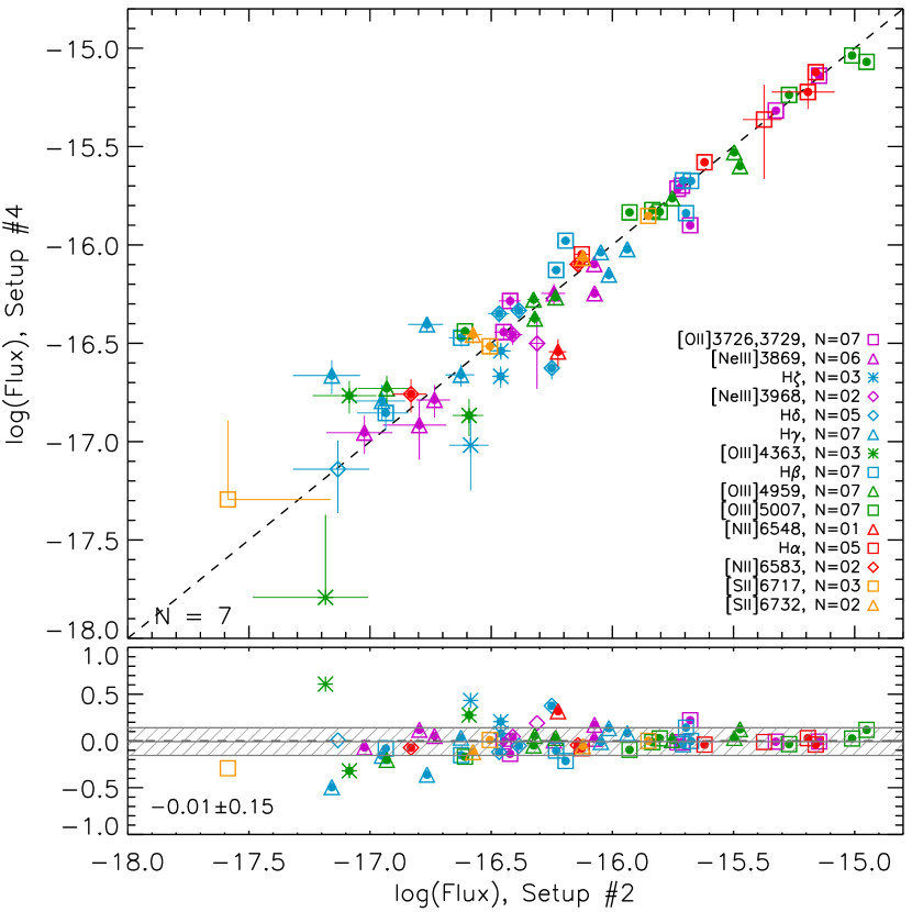
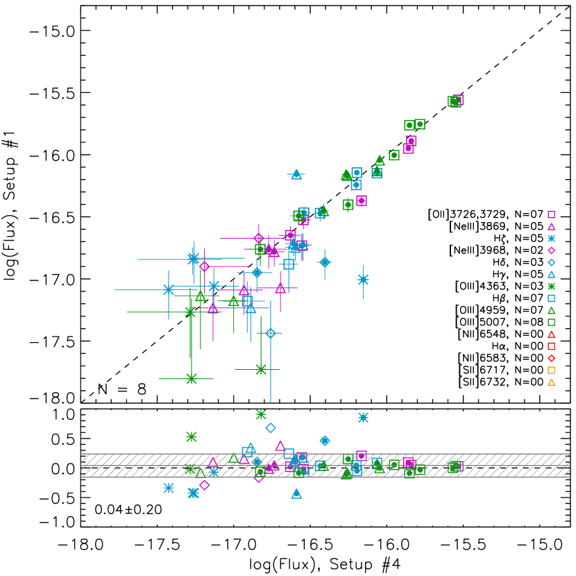
Figure 13.— Comparison between emission-line fluxes for various MMT setups. The top panels show the flux comparisons while the bottom panels show the differences against the flux. The different colors and symbols correspond to a given emission line (e.g., purple squares for [O ii] $\lambda\lambda$3726,3729). Measurements that are reliable at $\geq$3$\sigma$ in both spectra are marked with filled circles. The shaded grey regions in the bottom panels show the median and $\pm 1\sigma$. The median is computed using only $\geq$3$\sigma$ measurements.

Appendix B Rest-frame Optical Spectra for [O iii] $\lambda$4363 Galaxies

Here, we provide the rest-frame optical spectra for our sample of 20 galaxies in Figures 14–16. These plots are limited to a rest-frame wavelengths of 3400Å–5050Å. Our figures are limited toward lower fluxes to show the weak emission lines. Since the strong lines are saturated in these figures, we refer readers to Table 3, which provides the emission-line strengths. Overlaid in blue on these spectra are the locations of OH sky-lines with the OH line strengths indicated by the darkness of the blue shades. We also overlay strong and weak nebular emission lines in red. We previously discussed in Section 2.2 the acquisition and reduction of these spectra, and will discuss the absolute flux calibration of our spectra in Appendix A.

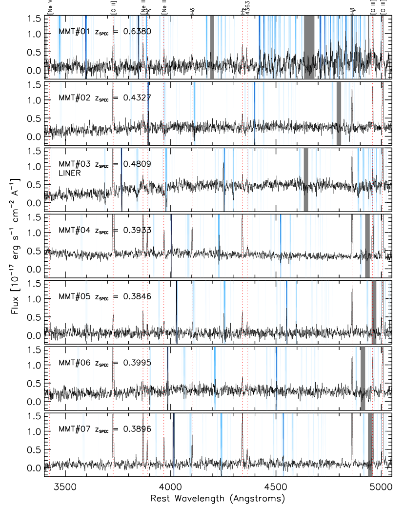
Figure 14.— MMT/Hectospec spectra for seven galaxies with full spectral coverage and detection of [O iii] $\lambda$4363 at $\geq$3$\sigma$. The most common nebular emission lines between 3400Å and 5010Å are denoted by the red dashed lines. OH sky-lines are indicated by blue vertical bands where the strength of the sky-lines is denoted by their shade of blue (darker is stronger). Grey shaded regions are those affected by atmospheric absorption (A- and B-bands).

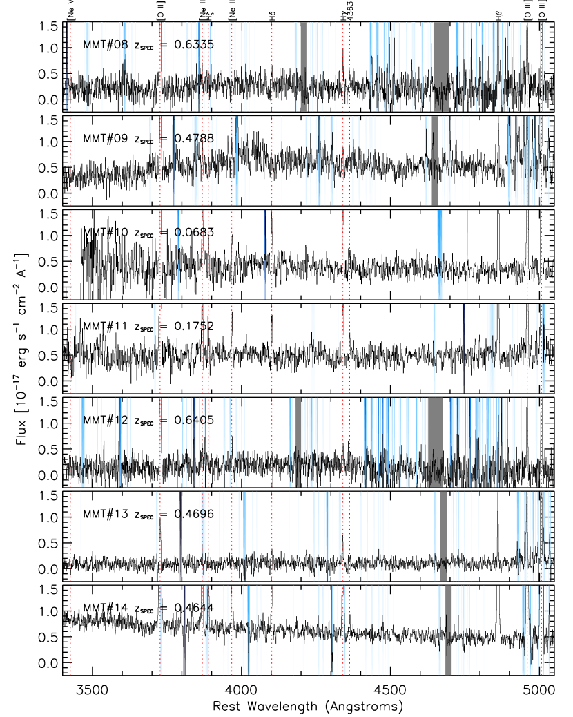
Figure 15.— Same as Figure 14 but for another seven galaxies observed with MMT/Hectospec.

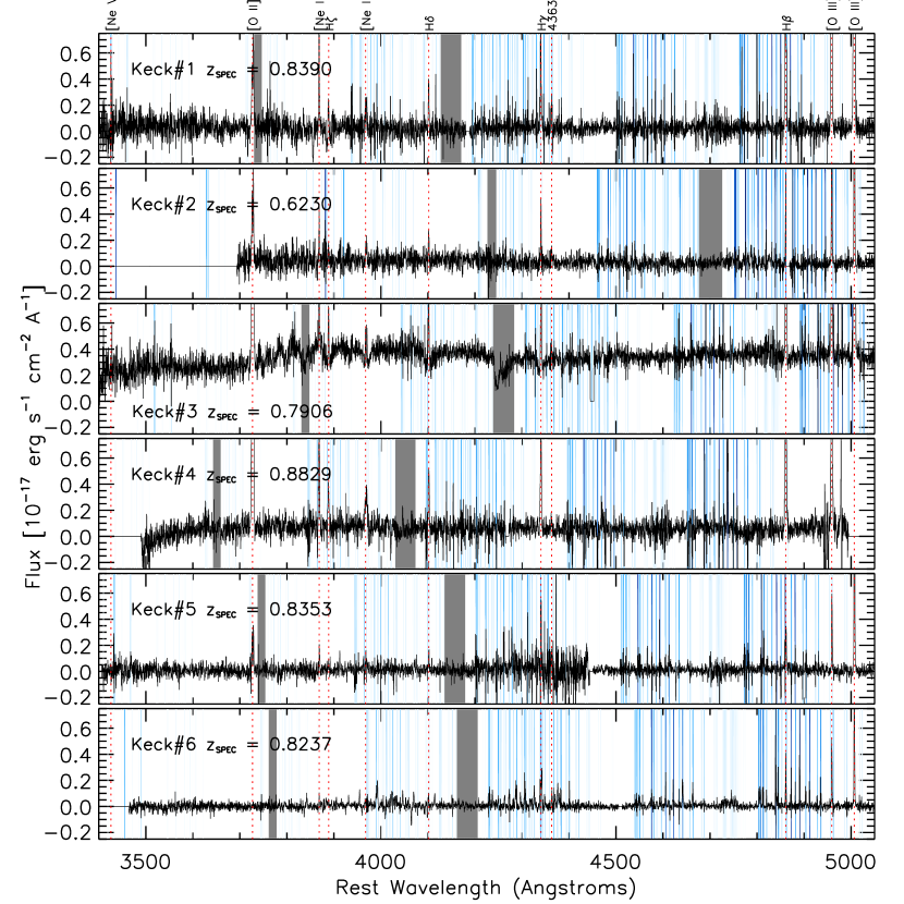
Figure 16.— Keck/DEIMOS spectra for six galaxies with full spectra coverage and detection of [O iii] $\lambda$4363 at $\geq$3$\sigma$. The most common nebular emission lines between 3400Å and 5010Å are denoted by the red dashed lines. OH sky-lines are indicated by blue vertical bands where the strength of the sky-lines is denoted by their shade of blue (darker is stronger). Grey shaded regions are those affected by atmospheric absorption (A- and B-bands).

References

- Allende Prieto et al. (2001) Allende Prieto, C., Lambert, D. L., & Asplund, M. 2001, ApJ, 556, L63
- Aller (1984) Aller, L. H. 1984, Astrophysics and Space Science Library, (Dordrecht: Reidel)
- Andrews & Martini (2013) Andrews, B. H., & Martini, P. 2013, ApJ, 765, 140 [AM13]
- Atek et al. (2010) Atek, H., Malkan, M., McCarthy, P., et al. 2010, ApJ, 723, 104
- Atek et al. (2011) Atek, H., Siana, B., Scarlata, C., et al. 2011, ApJ, 743, 121
- Baldwin et al. (1981) Baldwin, A., Phillips, M. M., & Terlevich, R. 1981, PASP, 93, 817
- Berg et al. (2012) Berg, D. A., Skillman, E. D., Marble, A. R., et al. 2012, ApJ, 754, 98
- Bertin & Arnouts (1996) Bertin, E., & Arnouts, S. 1996, A&AS, 117, 393
- Brown et al. (2008) Brown, W. R., Kewley, L. J., & Geller, M. J. 2008, AJ, 135, 92
- Bruzual & Charlot (2003) Bruzual, G., & Charlot, S. 2003, MNRAS, 344, 1000
- Bundy et al. (2006) Bundy, K., Ellis, R. S., Conselice, C. J., et al. 2006, ApJ, 651, 120
- Calzetti et al. (2000) Calzetti, D., Armus, L., Bohlin, R. C., Kinney, A. L., Koornneef, J., & Storchi-Bergmann, T. 2000, ApJ, 533, 682 [C00]
- Cardamone et al. (2009) Cardamone, C., Schawinski, K., Sarzi, M., et al. 2009, MNRAS, 399, 1191
- Chabrier (2003) Chabrier, G. 2003, PASP, 115, 763 [Chabrier]
- Davé et al. (2011) Davé, R., Finlator, K., & Oppenheimer, B. D. 2011, MNRAS, 416, 1354
- Davis et al. (2003) Davis, M., Faber, S. M., Newman, J., et al. 2003, Proc. SPIE, 4834, 161
- Dekel et al. (2009) Dekel, A., Birnboim, Y., Engel, G., et al. 2009, Nature, 457, 451
- Dickinson et al. (2003) Dickinson, M., Papovich, C., Ferguson, H. C., & Budavári, T. 2003, ApJ, 587, 25
- Ellison et al. (2008) Ellison, S. L., Patton, D. R., Simard, L., & McConnachie, A. W. 2008, ApJ, 672, L107
- Erb et al. (2006) Erb, D. K., Shapley, A. E., Pettini, M., et al. 2006, ApJ, 644, 813
- Faber et al. (2003) Faber, S. M., Phillips, A. C., Kibrick, R. I., et al. 2003, Proc. SPIE, 4841, 1657
- Fabricant et al. (2005) Fabricant, D., Fata, R., Roll, J., et al. 2005, PASP, 117, 1411
- Fabricant et al. (2008) Fabricant, D. G., Kurtz, M. J., Geller, M. J., et al. 2008, PASP, 120, 1222
- Ferland et al. (1998) Ferland, G. J., Korista, K. T., Verner, D. A., et al. 1998, PASP, 110, 761
- Fujita et al. (2003) Fujita, S. S., Ajiki, M., Shioya, Y., et al. 2003, ApJ, 586, L115
- Hainline et al. (2009) Hainline, K. N., Shapley, A. E., Kornei, K. A., et al. 2009, ApJ, 701, 52
- Hayashi et al. (2009) Hayashi, M., Motohara, K., Shimasaku, K., et al. 2009, ApJ, 691, 140
- Heckman (1980) Heckman, T. M. 1980, A&A, 87, 152
- Henry et al. (2013) Henry, A., Martin, C. L., Finlator, K., & Dressler, A. 2013, ApJ, 769, 148
- Hopkins (2004) Hopkins, A. M. 2004, ApJ, 615, 209
- Hoyos et al. (2005) Hoyos, C., Koo, D. C., Phillips, A. C., Willmer, C. N. A., & Guhathakurta, P. 2005, ApJ, 635, L21
- Hu et al. (2009) Hu, E. M., Cowie, L. L., Kakazu, Y., & Barger, A. J. 2009, ApJ, 698, 2014
- Izotov et al. (1999) Izotov, Y. I., Chaffee, F. H., Foltz, C. B., et al. 1999, ApJ, 527, 757
- Izotov et al. (1990) Izotov, I. I., Guseva, N. G., Lipovetskii, V. A., Kniazev, A. I., & Stepanian, J. A. 1990, Nature, 343, 238
- Izotov et al. (2006a) Izotov, Y. I., Stasińska, G., Meynet, G., Guseva, N. G., & Thuan, T. X. 2006a, A&A, 448, 955
- Izotov et al. (2006b) Izotov, Y. I., Schaerer, D., Blecha, A., et al. 2006b, A&A, 459, 71
- Izotov et al. (2011) Izotov, Y. I., Guseva, N. G., & Thuan, T. X. 2011, ApJ, 728, 161
- Izotov et al. (2012a) Izotov, Y. I., Thuan, T. X., & Guseva, N. G. 2012a, A&A, 546, A122
- Izotov et al. (2012b) Izotov, Y. I., Thuan, T. X., & Privon, G. 2012b, MNRAS, 427, 1229
- Jiang et al. (2013) Jiang, L., Egami, E., Mechtley, M., et al. 2013, ApJ, 772, 99
- Juneau et al. (2011) Juneau, S., Dickinson, M., Alexander, D. M., & Salim, S. 2011, ApJ, 736, 104
- Kakazu et al. (2007) Kakazu, Y., Cowie, L. L., & Hu, E. M. 2007, ApJ, 668, 853
- Kauffmann et al. (2003) Kauffmann, G., Heckman, T. M., Tremonti, C., et al. 2003, MNRAS, 346, 1055
- Kashikawa et al. (2006) Kashikawa, N., Shimasaku, K., Malkan, M. A., et al. 2006, ApJ, 648, 7
- Kashikawa et al. (2011) Kashikawa, N., Shimasaku, K., Matsuda, Y., et al. 2011, ApJ, 734, 119
- Kashikawa et al. (2004) Kashikawa, N., Shimasaku, K., Yasuda, N., et al. 2004, PASJ, 56, 1011
- Kennicutt (1998a) Kennicutt, R. C. 1998a, ARA&A, 36, 189
- Kennicutt (1998b) Kennicutt, R. C., Jr. 1998b, ApJ, 498, 541
- Kennicutt et al. (2008) Kennicutt, R. C., Jr., Lee, J. C., Funes, S. J., José G., Sakai, S., & Akiyama, S. 2008, ApJS, 178, 247
- Kereš et al. (2005) Kereš, D., Katz, N., Weinberg, D. H., & Davé, R. 2005, MNRAS, 363, 2
- Kewley et al. (2006) Kewley, L. J., Geller, M. J., & Barton, E. J. 2006, AJ, 131, 2004
- Kewley & Ellison (2008) Kewley, L. J., & Ellison, S. L. 2008, ApJ, 681, 1183
- Kewley et al. (2013) Kewley, L. J., Maier, C., Yabe, K., et al. 2013, ApJ, 774, L10
- Kniazev et al. (2003) Kniazev, A. Y., Grebel, E. K., Hao, L., et al. 2003, ApJ, 593, L73
- Kobulnicky & Kewley (2004) Kobulnicky, H. A., & Kewley, L. J. 2004, ApJ, 617, 240
- Kriek et al. (2009) Kriek, M., van Dokkum, P. G., Labbé, I., Franx, M., Illingworth, G. D., Marchesini, D., & Quadri, R. F. 2009, ApJ, 700, 221
- Kroupa (2001) Kroupa, P. 2001, MNRAS, 322, 231
- Lara-López et al. (2010) Lara-López, M. A., Cepa, J., Bongiovanni, A., et al. 2010, A&A, 521, L53
- Lee et al. (2006) Lee, H., Skillman, E. D., Cannon, J. M., et al. 2006, ApJ, 647, 970
- Lee et al. (2004) Lee, J. C., Salzer, J. J., & Melbourne, J. 2004, ApJ, 616, 752
- Lee et al. (2009) Lee, J. C., Gil de Paz, A., Tremonti, C., et al. 2009, ApJ, 706, 599
- Lee et al. (2012) Lee, J. C., Ly, C., Spitler, L., et al. 2012, PASP, 124, 782
- Leitherer et al. (1999) Leitherer, C., Schaerer, D., Goldader, J. D., et al. 1999, ApJS, 123, 3
- Ly et al. (2007) Ly, C., Malkan, M. A., Kashikawa, N., et al. 2007, ApJ, 657, 738 [L07]
- Ly et al. (2009) Ly, C., Malkan, M. A., Treu, T., et al. 2009, ApJ, 697, 1410
- Ly et al. (2011a) Ly, C., Malkan, M. A., Hayashi, M., et al. 2011a, ApJ, 735, 91
- Ly et al. (2011b) Ly, C., Lee, J. C., Dale, D. A., et al. 2011b, ApJ, 726, 109
- Ly et al. (2012a) Ly, C., Malkan, M. A., Kashikawa, N., et al. 2012a, ApJ, 747, L16
- Ly et al. (2012b) Ly, C., Malkan, M. A., Kashikawa, N., et al. 2012b, ApJ, 757, 63
- Madau (1995) Madau, P. 1995, ApJ, 441, 18
- Mannucci et al. (2010) Mannucci, F., Cresci, G., Maiolino, R., Marconi, A., & Gnerucci, A. 2010, MNRAS, 408, 2115
- Markwardt (2009) Markwardt, C. B. 2009, Astronomical Data Analysis Software and Systems XVIII, 411, 251
- Martin et al. (2012) Martin, C. L., Shapley, A. E., Coil, A. L., et al. 2012, ApJ, 760, 127
- Martin et al. (2005) Martin, D. C., Fanson, J., Schiminovich, D., et al. 2005, ApJ, 619, L1
- Mihos & Hernquist (1996) Mihos, J. C., & Hernquist, L. 1996, ApJ, 464, 641
- Miyazaki et al. (2002) Miyazaki, S., Komiyama, Y., Sekiguchi, M., et al. 2002, PASJ, 54, 833
- Morales-Luis et al. (2011) Morales-Luis, A. B., Sánchez Almeida, J., Aguerri, J. A. L., & Muñoz-Tuñón, C. 2011, ApJ, 743, 77
- Momcheva et al. (2013) Momcheva, I. G., Lee, J. C., Ly, C., et al. 2013, AJ, 145, 47
- Moustakas et al. (2011) Moustakas, J., Zaritsky, D., Brown, M., et al. 2011, ApJ, submitted (arXiv:1112.3300)
- Nagao et al. (2006) Nagao, T., Maiolino, R., & Marconi, A. 2006, A&A, 459, 85
- Nagao et al. (2008) Nagao, T., Sasaki, S. S., Maiolino, R., et al. 2008, ApJ, 680, 100
- Nakajima et al. (2013) Nakajima, K., Ouchi, M., Shimasaku, K., et al. 2013, ApJ, 769, 3
- Nicholls et al. (2012) Nicholls, D. C., Dopita, M. A., & Sutherland, R. S. 2012, ApJ, 752, 148
- Nicholls et al. (2013) Nicholls, D. C., Dopita, M. A., Sutherland, R. S., Kewley, L. J., & Palay, E. 2013, ApJS, 207, 21
- Noeske et al. (2007) Noeske, K. G., Weiner, B. J., Faber, S. M., et al. 2007, ApJ, 660, L43
- Oke (1974) Oke, J. B. 1974, ApJS, 27, 21
- Ouchi et al. (2004) Ouchi, M., Shimasaku, K., Okamura, S., et al. 2004, ApJ, 611, 660
- Pagel et al. (1979) Pagel, B. E. J., Edmunds, M. G., Blackwell, D. E., Chun, M. S., & Smith, G. 1979, MNRAS, 189, 95
- Pirzkal et al. (2013) Pirzkal, N., Rothberg, B., Ly, C., et al. 2013, ApJ, 772, 48
- Probst et al. (2008) Probst, R. G., George, J. R., Daly, P. N., Don, K., & Ellis, M. 2008, Proc. SPIE, 7014, 70142S
- Rigby et al. (2011) Rigby, J. R., Wuyts, E., Gladders, M. D., Sharon, K., & Becker, G. D. 2011, ApJ, 732, 59
- Rudnick et al. (2003) Rudnick, G., Rix, H.-W., Franx, M., et al. 2003, ApJ, 599, 847
- Rupke et al. (2010) Rupke, D. S. N., Kewley, L. J., & Barnes, J. E. 2010, ApJ, 710, L156
- Salpeter (1955) Salpeter, E. E. 1955, ApJ, 121, 161 [Salpeter]
- Savaglio et al. (2004) Savaglio, S., Glazebrook, K., Abraham, R. G., et al. 2004, ApJ, 602, 51
- Searle & Sargent (1972) Searle, L., & Sargent, W. L. W. 1972, ApJ, 173, 25
- Stetson (1987) Stetson, P. B. 1987, PASP, 99, 191
- Tremonti et al. (2004) Tremonti, C. A., Heckman, T. M., Kauffmann, G., et al. 2004, ApJ, 613, 898
- van der Wel et al. (2011) van der Wel, A., Straughn, A. N., Rix, H.-W., et al. 2011, ApJ, 742, 111
- Weiner et al. (2009) Weiner, B. J., Coil, A. L., Prochaska, J. X., et al. 2009, ApJ, 692, 187
- Wirth et al. (2004) Wirth, G. D., Willmer, C. N. A., Amico, P., et al. 2004, AJ, 127, 3121
- Xia et al. (2012) Xia, L., Malhotra, S., Rhoads, J., et al. 2012, AJ, 144, 28
- Yagi et al. (2002) Yagi, M., Kashikawa, N., Sekiguchi, M., Doi, M., Yasuda, N., Shimasaku, K., & Okamura, S. 2002, AJ, 123, 66
- York et al. (2000) York, D. G., Adelman, J., Anderson, J. E., Jr., et al. 2000, AJ, 120, 1579
- Yuan & Kewley (2009) Yuan, T.-T., & Kewley, L. J. 2009, ApJ, 699, L161