Legendrian Contact Homology in the Boundary of a Subcritical Weinstein $4$-Manifold

Abstract.

We give a combinatorial description of the Legendrian contact homology algebra associated to a Legendrian link in $S^{1}\times S^{2}$ or any connected sum $\#^{k}(S^{1}\times S^{2})$, viewed as the contact boundary of the Weinstein manifold obtained by attaching 1-handles to the 4-ball. In view of the surgery formula for symplectic homology [5], this gives a combinatorial description of the symplectic homology of any 4-dimensional Weinstein manifold (and of the linearized contact homology of its boundary). We also study examples and discuss the invariance of the Legendrian homology algebra under deformations, from both the combinatorial and the analytical perspectives.

1. Introduction

Legendrian contact homology is a part of Symplectic Field Theory, which is a generalization of Gromov–Witten theory to a certain class of noncompact symplectic manifolds including symplectizations of contact manifolds. SFT contains holomorphic curve theories for contact geometry, where Legendrian contact homology in a sense is the most elementary building block. Although Legendrian contact homology is a holomorphic curve theory, it is often computable as the homology of a differential graded algebra (DGA) that can be described more simply and combinatorially. For example, the DGA of a Legendrian $(n-1)$-link in the contact $(2n-1)$-sphere at the boundary of a symplectic $2n$-ball can be computed in terms of Morse flow trees, see [10].

In a different direction, the computation of Legendrian contact homology for 1-dimensional links in $\mathbb{R}^{3}$ was famously reduced by Chekanov [7] to combinatorics of polygons determined by the knot diagram of the link. The main goal of the current paper is to generalize this combinatorial description to Legendrian links in general boundaries of subcritical Weinstein $4$-manifolds. These boundaries are topologically connected sums $\#^{k}(S^{1}\times S^{2})$ of $k$ copies of $S^{1}\times S^{2}$ where $k$ is the rank of the first homology of the subcritical Weinstein $4$-manifold; we discuss Weinstein manifolds in more detail later in the introduction.

In Section 2.4, we present a combinatorial model for the Legendrian contact homology DGA for an arbitrary Legendrian link in $\#^{k}(S^{1}\times S^{2})$. This description follows Chekanov’s, but several new features are needed due to the presence of $1$-handles. Perhaps most notably, the DGA is generated by a countably infinite, rather than finite, set of generators (Reeb chords); cf. [29], where infinitely many Reeb chords also appear but in a different context. We accordingly present a generalization of the usual notion due to Chekanov of equivalence of DGAs, “stable tame isomorphism”, to the infinite setting. Briefly, Chekanov’s stable tame isomorphisms involve finitely many stabilizations and finitely many elementary automorphisms; here we allow compositions of infinitely many of both, as long as they behave well with respect to a filtration on the algebra.

One can view the combinatorial DGA abstractly as an invariant of Legendrian links in $\#^{k}(S^{1}\times S^{2})$, and indeed one can give a direct but somewhat involved algebraic proof that the DGA is invariant under Legendrian isotopy, without reference to holomorphic curves and contact homology. This is the content of Theorem 2.18 below. One can use the DGA, much as for Legendrian links in $\mathbb{R}^{3}$, to extract geometric information: e.g., the DGA provides an obstruction to Legendrian links in $\#^{k}(S^{1}\times S^{2})$ being destabilizable.

We then join the combinatorial and geometric sides of the story in our main result, Theorem 4.1, which states that the combinatorial DGA coincides with the DGA for Legendrian contact homology, defined via holomorphic disks. This result has interesting consequences for general 4-dimensional Weinstein manifolds that we discuss next.

One of the main motivations for the study undertaken in this paper is the surgery formula that expresses the symplectic homology of a Weinstein manifold in terms of the Legendrian contact homology of the attaching sphere of its critical handles, see [5]. Here, a Weinstein manifold is a $2n$-dimensional symplectic manifold $X$ which outside a compact subset agrees with $Y\times[0,\infty)$ for some contact $(2n-1)$-manifold $Y$ and which has the following properties. The symplectic form $\omega$ on $X$ is exact, $\omega=d\lambda$, and agrees with the standard symplectization form in the end $Y\times[0,\infty)$, $\lambda=e^{t}\alpha$, where $t\in[0,\infty)$ and $\alpha$ is a contact form on $Y$; and the Liouville vector field $Z$ $\omega$-dual to $\lambda$, $\omega(Z,\cdot)=\lambda$, is gradient-like for some Morse function $H\colon X\to\mathbb{R}$ with $H(y,t)=t$, $(y,t)\in Y\times[0,\infty)\subset X$. The zeros of $Z$ are then exactly the critical points of $H$ and the flow of $Z$ gives a finite handle decomposition for $X$. Furthermore, since $Z$ is a Liouville vector field, the unstable manifold of any zero of $Z$ is isotropic and hence the handles of $X$ have dimension at most $n$. The isotropic handles of dimension $<n$ are called subcritical and the Lagrangian handles of dimension $n$ critical.

A Weinstein manifold is called subcritical if all its handles are subcritical. The symplectic topology of subcritical manifolds is rather easy to control. More precisely, any subcritical Weinstein $2n$-manifold $X$ is symplectomorphic to a product $X^{\prime}\times\mathbb{R}^{2}$, where $X^{\prime}$ is a Weinstein $(2n-2)$-manifold, see [9, Section 14.4]. Furthermore, any symplectic tangential homotopy equivalence between two subcritical Weinstein manifolds is homotopic to a symplectomorphism, see [9, Sections 14.2–3]. As a consequence of these results, the nontrivial part of the symplectic topology of a Weinstein manifold is concentrated in its critical handles. More precisely, a Weinstein manifold $X$ is obtained from a subcritical Weinstein manifold $X_{0}$ by attaching critical handles along a collection of Legendrian attaching spheres $\Lambda\colon\bigsqcup_{j=1}^{m}S^{n-1}\to Y_{0}$, where $Y_{0}$ is the ideal contact boundary manifold of $X_{0}$. In particular, the Legendrian isotopy type of the link $\Lambda$ in $Y_{0}$ thus determines $X$ up to symplectomorphism.

An important invariant of a Weinstein manifold $X$ is its symplectic homology $SH(X)$, which is a certain limit of Hamiltonian Floer homologies for Hamiltonians with prescribed behavior at infinity. Symplectic homology and Legendrian contact homology are connected: [5, Corollary 5.7] expresses $SH(X)$ as the Hochschild homology of the Legendrian homology DGA $(\mathcal{A}(\Lambda),\partial(\Lambda))$ of the Legendrian attaching link $\Lambda$ of its critical handles. Similarly, the linearized contact homology of the ideal contact boundary of $X$ is expressed as the corresponding cyclic homology, see [5, Theorem 5.2].

In view of the above discussion, Theorem 4.1 then leads to a combinatorial formulation for the symplectic homology of any Weinstein 4-manifold (as well as the linearized contact homology of its ideal boundary). As one consequence, we deduce a new proof of a result of McLean [22] that states that there are exotic Stein structures on $\mathbb{R}^{8}$. We note that our construction of exotic Stein $\mathbb{R}^{8}$’s (and corresponding exotic contact $S^{7}$’s) is somewhat different from McLean’s.

Here is an outline of the paper. Our combinatorial setup and computation of the DGA are presented in Section 2 and sample calculations and applications are given in Section 3. In Section 4, we set up the contact topology needed to define Legendrian contact homology in our context. This leads to the proof in Section 5 that the combinatorial formula indeed agrees with the holomorphic curve count in the definition of the DGA. In the Appendices, we demonstrate invariance of the DGA under Legendrian isotopy in two ways: from the analytical perspective in Appendix A, and from the combinatorial perspective in Appendix B, which also includes a couple of deferred proofs of results from Section 2. It should be mentioned that the analytical invariance proof depends on a perturbation scheme for so-called M-polyfolds (the most basic level of polyfolds), the details of which are not yet worked out.

Acknowledgments

We thank Mohammed Abouzaid, Paul Seidel, and Ivan Smith for many helpful discussions. TE was partially supported by the Knut and Alice Wallenberg Foundation as a Wallenberg scholar. LN thanks Uppsala University for its hospitality during visits in 2009, when this project began, and 2010. LN was partially supported by NSF grants DMS-0706777 and DMS-0846346.

2. Combinatorial definition of the invariant

In this section, we present a combinatorial definition of the DGA for the Legendrian contact homology of a Legendrian link in $\#^{k}(S^{1}\times S^{2})$ with the usual Stein-fillable contact structure. (For the purposes of this paper, “link” means “knot or link”.) We first define a “normal form” in Section 2.1 for presenting Legendrian links in $\#^{k}(S^{1}\times S^{2})$, and describe an easy algorithm in Section 2.2 for deducing a normal form from the front of a Legendrian link, akin to the resolution procedure from [27]. We then define the DGA associated to a Legendrian link in normal form, in two parts: in Section 2.3 we present a differential subalgebra, the “internal DGA”, which is associated to the portion of the link inside the $1$-handles and depends only on the number of strands of the link passing through each $1$-handle; then we extend this in Section 2.4 to a DGA that takes account of the rest of the Legendrian link, with an example in Section 2.5. Finally, in Section 2.6 we present a version of stable tame isomorphism, an equivalence relation on DGAs, which allows us to state the algebraic invariance result for the DGA.

2.1. Normal form for the $xy$ projection of a Legendrian link

As is the case in $\mathbb{R}^{3}$, it is most convenient to define the DGA for a Legendrian link in $\#^{k}(S^{1}\times S^{2})$ in terms of the projection of the link (or the portion outside of the $1$-handles) in the $xy$ plane. Let $A,M>0$.

Definition 2.1.

A tangle in $[0,A]\times[-M,M]\times[-M,M]$ is Legendrian if it is everywhere tangent to the standard contact structure $dz-y\,dx$, where $x,y,z$ are the usual coordinates. A Legendrian tangle $\Lambda\subset[0,A]\times[-M,M]\times[-M,M]$ is in normal form if there exist integers $n_{1},\ldots,n_{k}\geq 0$ such that

$$\Lambda\cap\{x=0\} =\{(0,y_{i}^{\ell},z_{i}^{\ell})\,|\,1\leq\ell\leq k,~{}1\leq i\leq n_{\ell}\},$$

$$\Lambda\cap\{x=A\} =\{(A,\tilde{y}_{i}^{\ell},\tilde{z}_{i}^{\ell})\,|\,1\leq\ell\leq k,~{}1\leq i\leq n_{\ell}\},$$

with $y_{i}^{\ell},z_{i}^{\ell},\tilde{y}_{i}^{\ell},\tilde{z}_{i}^{\ell}\in[-M,M]$ satisfying the following conditions:

• For some (arbitrarily small) $\epsilon>0$, for any fixed $\ell$, each of the following sets lies in an interval of length less than $\epsilon$: $\{y_{1}^{\ell},\ldots,y_{n_{\ell}}^{\ell}\}$, $\{z_{1}^{\ell},\ldots,z_{n_{\ell}}^{\ell}\}$, $\{\tilde{y}_{1}^{\ell},\ldots,\tilde{y}_{n_{\ell}}^{\ell}\}$, and $\{\tilde{z}_{1}^{\ell},\ldots,\tilde{z}_{n_{\ell}}^{\ell}\}$;

• if $\ell_{1}<\ell_{2}$ then for all $i,j$,

  $$y_{i}^{\ell_{1}} >y_{j}^{\ell_{2}}, z_{i}^{\ell_{1}} >z_{j}^{\ell_{2}},$$

  $$\tilde{y}_{i}^{\ell_{1}} >\tilde{y}_{j}^{\ell_{2}}, \tilde{z}_{i}^{\ell_{1}} >\tilde{z}_{j}^{\ell_{2}};$$

• for $1\leq i<j\leq n_{\ell}$,

  $$y_{i}^{\ell} >y_{j}^{\ell}, z_{i}^{\ell} >z_{j}^{\ell},$$

  $$\tilde{y}_{i}^{\ell} <\tilde{y}_{j}^{\ell}, \tilde{z}_{i}^{\ell} >\tilde{z}_{j}^{\ell}.$$

Less formally, $\Lambda$ meets $x=0$ and $x=A$ in $k$ groups of strands, with groups of size $n_{1},\ldots,n_{k}$. The groups are arranged from top to bottom in both the $xy$ and the $xz$ projections. Within the $\ell^{\rm th}$ group, the strands can be labeled by $1,\ldots,n_{\ell}$ in such a way that the strands appear in increasing order from top to bottom in both the $xy$ and $xz$ projections at $x=0$ and in the $xz$ projection at $x=A$, and from bottom to top in the $xy$ projection at $x=A$.

Any Legendrian tangle in normal form corresponds to a Legendrian link in $\#^{k}(S^{1}\times S^{2})$ by attaching $k$ $1$-handles joining the portions of the $xz$ projection of the tangle at $x=0$ to the portions at $x=A$. The $\ell^{\rm th}$ $1$-handle joins the $\ell^{\rm th}$ group at $x=0$ to the $\ell^{\rm th}$ group at $x=A$, and within this group, the strands with the same label at $x=0$ and $x=A$ are connected through the $1$-handle.

See Figure 1 for an illustration of the $xy$ and $xz$ projections of a Legendrian tangle in normal form. Note that the $xy$ projection can be deduced from the $xz$ projection as usual by setting $y=dz/dx$.

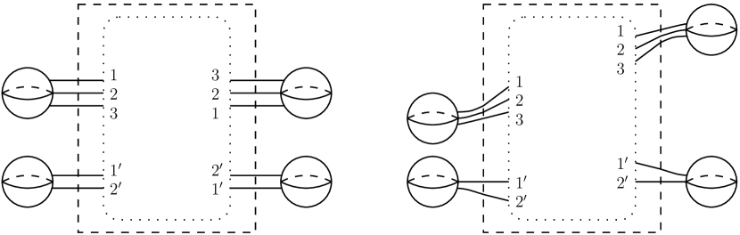
Figure 1. The $xy$ (left) and $xz$ (right) projections of a Legendrian tangle in normal form. The dashed boxes are $[0,A]\times[-M,M]$ in $(x,y)$ or $(x,z)$ coordinates, and the tangle continues into the dotted boxes. In the terminology of Definition 2.1, the strands labeled $1$, $2$, $3$ intersect the left side of the dashed boxes at $(0,y_{1}^{1},z_{1}^{1})$, $(0,y_{2}^{1},z_{2}^{1})$, $(0,y_{3}^{1},z_{3}^{1})$ and the right side at $(A,\tilde{y}_{1}^{1},\tilde{z}_{1}^{1})$, $(A,\tilde{y}_{2}^{1},\tilde{z}_{2}^{1})$, $(A,\tilde{y}_{3}^{1},\tilde{z}_{3}^{1})$, respectively; strands $1^{\prime}$, $2^{\prime}$ intersect the left side at $(0,y_{1}^{2},z_{1}^{2})$, $(0,y_{2}^{2},z_{2}^{2})$ and the right side at $(A,\tilde{y}_{1}^{2},\tilde{z}_{1}^{2})$, $(A,\tilde{y}_{2}^{2},\tilde{z}_{2}^{2})$.

Definition 2.2.

A tangle diagram is in $xy$-normal form if it is the $xy$ projection of a Legendrian tangle in normal form.

In Section 2.4, we will associate a differential graded algebra to a tangle diagram in $xy$-normal form.

2.2. Resolution

As in the case of $\mathbb{R}^{3}$ [7], it is not necessarily easy to tell whether a tangle diagram is (planar isotopic to a diagram) in $xy$-normal form. However, in practice a Legendrian link in $\#^{k}(S^{1}\times S^{2})$ is typically presented as a front diagram, following Gompf [19]. In this subsection, we describe a procedure called resolution that inputs a front diagram for a Legendrian link in $\#^{k}(S^{1}\times S^{2})$, and outputs a tangle diagram in $xy$-normal form that represents a Legendrian-isotopic link.

Gompf represents a Legendrian link in $\#^{k}(S^{1}\times S^{2})$ by a front diagram in a box $[0,A]\times[-M,M]$ that is nearly identical in form to the $xz$ projections of our normal-form tangles from Definition 2.1, but with the intersections with $x=0$ and $x=A$ aligned horizontally; see Figure 2 for an illustration. We say that such a front is in Gompf standard form.

2pt tangle at 127 64 tangle at 415 64

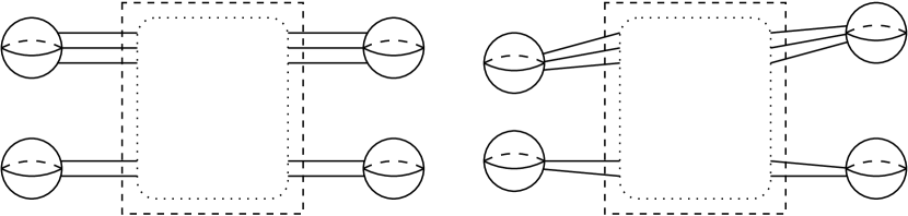
Figure 2. A Legendrian front diagram in $\#^{2}(S^{1}\times S^{2})$ in Gompf standard form (left), and perturbed to be the $xz$ projection of a tangle in normal form in the sense of Definition 2.1 (right).

Any front in Gompf standard form can be perturbed to be the $xz$ projection of a tangle in normal form. This merely involves perturbing the portions of the front near $x=0$ and $x=A$ so that, rather than being horizontal, they are nearly horizontal but with slopes increasing from bottom to top along $x=0$, and increasing from bottom to top along $x=A$ except decreasing within each group of strands corresponding to a $1$-handle. The resulting front then gives a Legendrian tangle whose $xy$ projection satisfies the ordering condition of Definition 2.1. See Figure 2.

Although one can deduce the $xy$ projection of a Legendrian tangle from its $xz$ projection by using $y=dz/dx$, this can be somewhat difficult to effect in practice. However, as in $\mathbb{R}^{3}$ [27], if we allow the tangle to vary by Legendrian isotopy (in fact, planar isotopy in the $xz$ plane), then it is possible to obtain a front whose corresponding $xy$ projection is easy to describe.

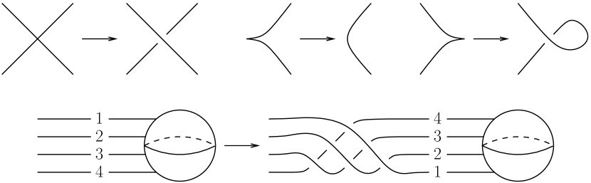
Figure 3. Resolving a front in Gompf standard form.

Definition 2.3.

The resolution of a front in Gompf standard form is the tangle diagram obtained by resolving the singularities of the front as shown in Figure 3 and, for each $1$-handle, adding a half-twist to the strands that pass through that $1$-handle at the $x=A$ end of the tangle.

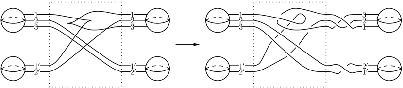
Figure 4. Example of front resolution for a Legendrian link in $\#^{2}(S^{1}\times S^{2})$.

Note that the half-twist has the effect of reversing the order of the strands entering the $1$-handles at $x=A$. In Gompf standard form, the strands entering a $1$-handle from the left and the right are identified with each other in the obvious way, by identifying $x=0$ and $x=A$; in the resolution of such a front, the top strand entering a particular $1$-handle from the left is identified with the bottom strand entering the $1$-handle from the right, and so forth. See Figure 4 for an example of a resolution.

Proposition 2.4.

Let $\Lambda$ be a Legendrian link in $\#^{k}(S^{1}\times S^{2})$ represented by a front in Gompf standard form. Then the resolution of the front is (up to planar isotopy) the $xy$ projection of a Legendrian link in normal form that is Legendrian isotopic to $\Lambda$.

See Appendix B.1 for the proof of Proposition 2.4, which is very similar to the analogous proof for resolutions in $\mathbb{R}^{3}$ from [27].

In practice, to compute the DGA associated to a Legendrian link in $\#^{k}(S^{1}\times S^{2})$, we begin with a Gompf standard form for the link, resolve it as above, and then apply the combinatorial formula for the DGA to be described in Section 2.4 below.

2.3. Internal differential graded algebra

Here we present the subalgebra of the contact homology differential graded algebra determined by the Reeb chords in each $1$-handle, and holomorphic disks with positive puncture at one of these Reeb chords. Let $n\geq 1$ be an integer, representing the number of strands of the Legendrian link $\Lambda=\Lambda_{1}\cup\dots\cup\Lambda_{s}$ passing through the $1$-handle, where the $\Lambda_{j}$ denote the knot components of $\Lambda$. To define a grading on the subalgebra, we need two auxiliary pieces of data: an $s$-tuple of integers $(r_{1},\ldots,r_{s})$ associated to the components $\Lambda_{j}$, $j=1,\dots,s$, and an $n$-tuple of integers $(m(1),\ldots,m(n))$. These represent the rotation numbers of the Legendrian link (which only appear here in the grading of the homology variables $t_{j}$) and a choice of Maslov potential for each of the strands passing through the $1$-handle; see also Section 2.4.

Given $(r_{1},\dots,r_{s})$ and $(m(1),\ldots,m(n))$, let $(\mathcal{A}_{n},\partial_{n})$ denote the differential graded algebra given as follows. As an algebra, $\mathcal{A}_{n}$ is the tensor algebra over the coefficient ring $\mathbb{Z}[H_{1}(\Lambda)]$, that is,

$$\mathbb{Z}[\mathbf{t},\mathbf{t}^{-1}]:=\mathbb{Z}[t_{1},t_{1}^{-1},\dots,t_{s},t_{s}^{-1}],$$

freely generated by generators $c_{ij}^{0}$ for $1\leq i<j\leq n$ and $c_{ij}^{p}$ for $1\leq i,j\leq n$ and $p\geq 1$. (See Remark 5.2 for a discussion of the geometric significance of the coefficient ring.) This algebra is graded by setting $|t_{j}|=-2r_{j}$, $|t_{j}^{-1}|=2r_{j}$, and

$$|c_{ij}^{p}|=2p-1+m(i)-m(j)$$

for all $i,j,p$. The differential $\partial_{n}$ is defined on generators by

$$\partial_{n}(c_{ij}^{0}) =\sum_{m=1}^{n}\sigma_{i}\sigma_{m}c_{im}^{0}c_{mj}^{0}$$

$$\partial_{n}(c_{ij}^{1}) =\delta_{ij}+\sum_{m=1}^{n}\sigma_{i}\sigma_{m}c_{im}^{0}c_{mj}^{1}+\sum_{m=1}^{n}\sigma_{i}\sigma_{m}c_{im}^{1}c_{mj}^{0}$$

$$\partial_{n}(c_{ij}^{p}) =\sum_{\ell=0}^{p}\sum_{m=1}^{n}\sigma_{i}\sigma_{m}c_{im}^{\ell}c_{mj}^{p-\ell}$$

where $p\geq 2$, $\sigma_{i}=(-1)^{m(i)}$ for all $i$, $\delta_{ij}$ is the Kronecker delta, and we set $c_{ij}^{0}=0$ for $i\geq j$. Extend $\partial_{n}$ to all of $\mathcal{A}_{n}$ in the usual way by the Leibniz rule

$$\partial_{n}(xy)=(\partial_{n}x)y+(-1)^{|x|}x(\partial_{n}y).$$

It is clear that $\partial_{n}$ has degree $-1$, and easy to check that $\partial_{n}^{2}=0$. Note that $\mathcal{A}_{n}$ is infinitely generated as an algebra but has a natural increasing filtration given by the superscripts, with respect to which $\partial_{n}$ is a filtered differential.

Given a Legendrian link $\Lambda\subset\#^{k}(S^{1}\times S^{2})$, we can associate a DGA $(\mathcal{A}_{n_{i}},\partial_{n_{i}})$ as above to each of the $k$ $1$-handles; see Section 2.4 below. We refer to the DGA whose generators are the collection of generators of $\mathcal{A}_{n_{i}}$, $i=1,\ldots,k$, and whose differential is induced from $\partial_{n_{i}}$, as the internal DGA of $\Lambda$.

2.4. The DGA for an $xy$ projection in normal form

We can now define the DGA associated to a Legendrian link in $\#^{k}(S^{1}\times S^{2})$, or more precisely to a tangle in $xy$-normal form in the terminology of Section 2.1, with one base point for each link component.

Suppose that we have a Legendrian link $\Lambda=\Lambda_{1}\cup\dots\cup\Lambda_{s}\subset\#^{k}(S^{1}\times S^{2})$ in normal form; then its projection $\pi_{xy}(\Lambda)$ to the $xy$ plane is a tangle diagram in $xy$-normal form. Let $a_{1},\dots,a_{n}$ denote the crossings of the tangle diagram. Label the $k$ $1$-handles appearing in the diagram by $1,\ldots,k$ from top to bottom; let $n_{\ell}$ denote the number of strands of the tangle passing through handle $\ell$. For each $\ell$, label the strands running into the $1$-handle on the left side of the diagram by $1,\ldots,n_{\ell}$ from top to bottom, and label the strands running into the $1$-handle on the right side by $1,\ldots,n_{\ell}$ from bottom to top. Also choose base points $\ast_{j}$, $j=1,\dots,s$ in the tangle diagram such that $\ast_{j}$ lies on component $\Lambda_{j}$ for all $j=1,\ldots,s$, and no $\ast_{j}$ lies at any of the crossings (or in the $1$-handles).

We can now define the DGA. Our definition involves three parts: the algebra, the grading, and the differential.

2.4.A. The algebra

Let $\mathcal{A}$ be the tensor algebra over $\mathbb{Z}[\mathbf{t},\mathbf{t}^{-1}]=\mathbb{Z}[t_{1},t_{1}^{-1},\dots,t_{s},t_{s}^{-1}]$ freely generated by:

• $a_{1},\ldots,a_{n}$;

• $c_{ij;\ell}^{0}$ for $1\leq\ell\leq k$ and $1\leq i<j\leq n_{\ell}$;

• $c_{ij;\ell}^{p}$ for $1\leq\ell\leq k$, $p>0$, and $1\leq i,j\leq n_{\ell}$.

(We will drop the index $j$ in $t_{j}$ when the Legendrian $\Lambda$ is a single-component knot, and the index $\ell$ in $c_{ij;\ell}^{p}$ when there is only one $1$-handle.) Note that $\mathcal{A}$ contains $k$ subalgebras $\mathcal{A}_{n_{1}}^{1},\ldots,\mathcal{A}_{n_{k}}^{k}$, where $\mathcal{A}_{n_{\ell}}^{\ell}$ is the tensor algebra over $\mathbb{Z}[\mathbf{t},\mathbf{t}^{-1}]$ freely generated by $c_{ij;\ell}^{0}$ for $1\leq i<j\leq n_{\ell}$ and $c_{ij;\ell}^{p}$ for $p>0$ and $1\leq i,j\leq n_{\ell}$. Each of these subalgebras $\mathcal{A}_{n_{\ell}}^{\ell}$ should be thought of as the internal DGA corresponding to the $\ell^{\rm th}$ handle, and the grading and differential on this subalgebra will be defined accordingly. Together, the $\mathcal{A}_{n_{\ell}}^{\ell}$ generate a differential subalgebra of $\mathcal{A}$, which we call “the” internal DGA of $\Lambda$.

It should be noted that we have chosen our formulation of the algebra in such a way that all of the $t^{\pm 1}_{j}$ commute with each other and with the generators $a_{i}$ and $c_{ij;\ell}^{p}$. This suffices for our purposes but is not strictly necessary. It is possible to elaborate on the construction and consider an algebra over $\mathbb{Z}$ generated by $a_{i}$, $c_{ij;\ell}^{p}$, and $t^{\pm 1}_{j}$, modulo only the obvious relations $t_{j}\cdot t_{j}^{-1}=t^{-1}_{j}\cdot t_{j}=1$. See, e.g., [14, Section 2.3.2] or [25, Remark 2.2] for more discussion.

2.4.B. Grading

The grading on $\mathcal{A}$ is determined by stipulating a grading on $t_{j}$ and on each generator $a_{i}$ and $c_{ij;\ell}^{p}$ of $\mathcal{A}$. We will do each of these in turn.

We begin with some preliminary definitions. A path in $\pi_{xy}(\Lambda)$ is a path that traverses some amount of $\pi_{xy}(\Lambda)$, connected except for points where it enters a $1$-handle (i.e., approaches $x=0$ or $x=A$ along a labeled strand) and exits the $1$-handle along the corresponding strand (i.e., departs $x=A$ or $x=0$ along the strand with the same label). In particular, the tangent vector in $\mathbb{R}^{2}$ to a path varies continuously as we traverse the path (note that the strands entering or exiting a $1$-handle are horizontal). The rotation number $r(\gamma)$ of a path $\gamma$ consisting of unit vectors in $\mathbb{R}^{2}$ (i.e., points in $S^{1}$) is the number of counterclockwise revolutions made by $\gamma(t)$ around $S^{1}$ as we traverse the path (i.e., the total curvature $\int_{\gamma}\kappa\,ds$ divided by $2\pi$); note that this is generally a real number, and is an integer if and only if $\gamma$ is closed. By slight abuse of notation, we will often speak of the rotation number of a path $\gamma$ in $\pi_{xy}(\Lambda)$ to mean the rotation number of its unit tangent vector $\gamma^{\prime}(t)/|\gamma^{\prime}(t)|$.

In this terminology, the rotation number $r_{j}=r(\Lambda_{j})$ is the rotation number of the path in $\pi_{xy}(\Lambda)$ that begins and ends at the base point $\ast_{j}$ on the $j^{\rm th}$ component $\Lambda_{j}$ and traverses the diagram once in the direction of the orientation of $\Lambda_{j}$. We define

$$|t_{j}|=-2r(\Lambda_{j}).$$

To define the remainder of the grading on $\mathcal{A}$, we need to make some auxiliary choices joining tangent directions to the various base points $\ast_{1},\ldots,\ast_{s}$, although the grading only depends on these choices in the case of multi-component links ($s\geq 2$). For $i=1,\ldots,s$, let $v_{i}\in S^{1}$ denote the unit tangent vector to the oriented curve $\pi_{xy}(\Lambda_{i})$ at the base point $\ast_{i}$. Now for $i=2,\ldots,s$, pick a path $\xi_{i}$ in $S^{1}$ from $v_{1}$ to $v_{i}$; then for $1\leq i,j\leq s$, let $\xi_{ij}$ denote the path in $S^{1}$ from $v_{i}$ to $v_{j}$ given by the orientation reverse of $\xi_{i}$ followed by $\xi_{j}$, considered up to homotopy (so we can choose $\xi_{ii}$ to be constant). Note that there is a $\mathbb{Z}^{s-1}$ worth of possible choices for the paths $\xi_{ij}$.

With $\xi_{ij}$ chosen, we next define the grading of the $a_{i}$ generators. Let $a_{i}^{+}$ and $a_{i}^{-}$ denote the preimages $a_{i}^{+}$ and $a_{i}^{-}$ in $\Lambda$ of the crossing point $a_{i}$ in the upper and lower strands of the crossing, respectively, and suppose that $a_{i}^{+},a_{i}^{-}$ belong to components $\Lambda_{i^{+}},\Lambda_{i^{-}}$, respectively. There are unique paths $\gamma^{\pm}$ in the $xy$ projection of the component $\Lambda_{i^{\pm}}$ connecting $a_{i}^{\pm}$ to the base point $\ast_{i^{\pm}}$ and following the orientation of $\Lambda_{i^{\pm}}$, such that the lifts of $\gamma^{\pm}$ to $\Lambda$ are embedded. Let $\sigma_{i}$ be the path of unit tangent vectors along $\gamma^{+}$, followed by $\xi_{j^{+}j^{-}}$, and followed by the path of unit tangent vectors along $\gamma^{-}$ traversed backwards. Assume that the crossing at $a_{i}$ is transverse (else perturb the diagram); then $r(\sigma_{i})$ is neither an integer nor a half-integer, and we define

$$|a_{i}|=\lfloor 2r(\sigma_{i})\rfloor,$$

where $\lfloor x\rfloor$ denotes the largest integer smaller than $x$.

It remains to define the grading of the $c_{ij;\ell}^{p}$ generators. This can be done by adding dips and treating $c_{ij;\ell}^{0}$ generators as crossings in a dipped diagram; cf. the proof of Proposition 2.8 in Appendix B.1. We however use a slightly different approach here. Choose a Maslov potential $m$ that associates an integer to each strand passing through each $1$-handle, in such a way that the following conditions hold:

• if $S_{L},S_{R}$ are strands on the left and right of $\pi_{xy}(\Lambda)$ that correspond to the ends of a strand of $\Lambda$ passing through a $1$-handle, then $m(S_{L})=m(S_{R})$, and these Maslov potentials are even if $\Lambda$ is oriented left to right (i.e., it passes through the $1$-handle from $x=A$ to $x=0$), and odd if $\Lambda$ is oriented right to left;

• if $S,S^{\prime}$ are endpoints of strands through $1$-handles with $S\in\Lambda_{i}$ and $S^{\prime}\in\Lambda_{j}$, such that $\Lambda_{i},\Lambda_{j}$ are oriented from $S,S^{\prime}$ to $\ast_{i},\ast_{j}$ respectively, then

  $$m(S^{\prime})-m(S)=-2r(\sigma)$$

  where $\sigma$ is the path of unit tangent vectors along $\Lambda_{i}$ from $S$ to $\ast_{i}$, followed by $\xi_{ij}$, followed by the path of unit tangent vectors along $\Lambda_{j}$ from $\ast_{j}$ to $S^{\prime}$; note that this last path is traversed opposite to the orientation on $\Lambda_{j}$, and that $r(\sigma)\in\frac{1}{2}\mathbb{Z}$ since strands are horizontal as they pass through $1$-handles.

It is easy to check that the Maslov potential is well-defined (given choices for $\xi_{ij}$) up to an overall shift by an even integer.

As suggested by Section 2.3, we now grade the “internal generators” $c_{ij;\ell}^{p}$ of $\mathcal{A}$ as follows:

$$|c_{ij;\ell}^{p}|=2p-1+m(S_{i;\ell})-m(S_{j;\ell}),$$

where $S_{i;\ell},S_{j;\ell}$ are the strands running through handle $\ell$ labeled by $i$ and $j$. This completes the definition of the grading on $\mathcal{A}$.

Remark 2.5.

Note that the grading on $\mathcal{A}$ is independent of the choice of Maslov potential. Different choices of $\gamma_{ij}$ do however lead to different gradings for $s\geq 2$. As mentioned previously, there is a $(2\mathbb{Z})^{s-1}$ worth of choices for $\xi_{ij}$. Given the grading $|\cdot|$ on $\mathcal{A}$ resulting from such a choice, and any $(2n_{1},\ldots,2n_{s})\in(2\mathbb{Z})^{s}$, one can obtain another grading $|\cdot|^{\prime}$ on $\mathcal{A}$ by defining

$$|a_{i}|^{\prime}=|a_{i}|+2(n_{i^{+}}-n_{i^{-}})$$

and similarly for the other generators $c_{ij;\ell}^{p}$. (The grading on the homology generators $t_{1},\ldots,t_{s}$ is unchanged.) Any such grading comes from a different choice of $\xi_{ij}$, and conversely.

Remark 2.6.

If $\pi_{xy}(\Lambda)$ is the resolution of a front diagram of an $s$-component link, then we can calculate the grading on generators of $\mathcal{A}$ directly from the front diagram, as follows. We can associate a Maslov potential to connected components of a front diagram minus cusps and the base points $\ast_{j}$, $1,\dots,s$, in such a way that the following conditions hold:

• the same Maslov potential is assigned to the left and right sides of the same strand (connected through a $1$-handle), and this potential is even if the strand is oriented left to right (from $x=A$ to $x=0$) and odd otherwise;

• at a cusp, the upper component (in the $z$ direction) has Maslov potential one more than the lower component.

As before, we set $|t_{j}|=-2r(\Lambda_{j})$ and $|c_{ij;\ell}^{p}|=2p-1+m(S_{i;\ell})-m(S_{j;\ell})$. The other generators of $\mathcal{A}$ are in one-to-one correspondence to: right cusps in the front; crossings in the front; and pairs of strands entering the same $1$-handle at $x=A$ (corresponding to the half-twists in the resolution). Let $a$ be one of these generators. If $a$ is a right cusp, define $|a|=1$ (this assumes that no base point $\ast_{j}$ is in the portion of the resolution given by the loop at $a$). If $a$ is a crossing, then $|a|=m(S_{o})-m(S_{u})$, where $S_{u}$ is the undercrossing strand at $a$ (in the front projection, i.e., the strand with more positive slope) and $S_{o}$ is the overcrossing strand at $a$. Finally, if $a$ is a crossing in the half-twist near a handle and involving strands labeled $i$ and $j$ with $i<j$, then

$$|a|=m(S_{i})-m(S_{j})$$

where $S_{i}$ and $S_{j}$ are the strands labeled $i$ and $j$ at the $1$-handle.

2.4.C. Differential

Finally, we define the differential $\partial$ on $\mathcal{A}$. It suffices to define the differential on generators of $\mathcal{A}$, and then impose the Leibniz rule. We set $\partial(t_{j})=\partial(t^{-1}_{j})=0$. On each $\mathcal{A}_{n_{\ell}}^{\ell}$, we then define the differential by $\partial=\partial_{n_{\ell}}$, as defined in Section 2.3.

It remains to define the differential for crossings $a_{i}$. To do this, decorate the quadrants of the crossings in $\pi_{xy}(\Lambda)$ by the “Reeb signs” shown in the left diagram in Figure 5, as in Chekanov [7].

Figure 5. Reeb signs on the left; orientation signs at a crossing $a$ on the right.

For $r\geq 0$, let $a_{i},b_{1},\ldots,b_{r}$ be a collection of (not necessarily distinct) generators of $\mathcal{A}$ such that $a_{i}$ is a crossing in $\pi_{xy}(\Lambda)$, and each of $b_{1},\ldots,b_{r}$ is either a crossing $a_{j}$ or a generator of the form $c_{j_{1}j_{2};\ell}^{0}$ for $j_{1}<j_{2}$. Define $\Delta(a_{i};b_{1},\ldots,b_{r})$ to be the set of immersed disks with convex corners (up to parametrization) with boundary on $\pi_{xy}(\Lambda)$, such that the corners of the disk are, in order as we traverse the boundary counterclockwise, a “positive corner” at $a_{i}$ and “negative corners” at each of $b_{1},\ldots,b_{r}$. Here positive and negative corners are as depicted in Figure 6. Disks are not allowed to pass through a $1$-handle, but they can have a negative corner $c_{j_{1}j_{2};\ell}^{0}$ on either side of the $1$-handle.

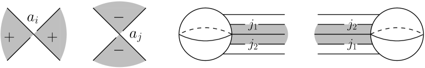
Figure 6. Positive and negative corners for a disk (locally depicted by one of the shaded regions). From left to right: two possible positive corners at a crossing $a_{i}$; two possible negative corners at $a_{j}$; and two possible negative corners at $c_{j_{1}j_{2};\ell}^{0}$, where $j_{1}<j_{2}$ and $\ell$ is the label of the depicted handle.

We now set

$$\partial(a_{i})=\sum_{r\geq 0}~{}\sum_{b_{1},\ldots,b_{r}}~{}\sum_{\Delta\in\Delta(a_{i};b_{1},\ldots,b_{r})}\operatorname{sgn}(\Delta)\,t_{1}^{-n_{1}(\Delta)}\cdots t_{s}^{-n_{s}(\Delta)}\,b_{1}\cdots b_{r},$$

where $n_{j}(\Delta)$ is the signed number of times that the boundary of $\Delta$ passes through $\ast_{j}$, and $\operatorname{sgn}(\Delta)$ is a sign to be defined below. Extend $\partial$ to $\mathcal{A}$ via the Leibniz rule. For any crossing $a_{i}$, the set of all possible immersed disks with $+$ corner at $a_{i}$ and any number of $-$ corners is finite, by the usual area argument (or see the proof of Proposition 2.8 below), and so the sum in $\partial(a_{i})$ is finite.

To define the sign associated to an immersed disk, we assign “orientation signs” (entirely distinct from Reeb signs) at every corner of the disk, as follows. For corners at a $c_{j_{1}j_{2};\ell}^{0}$, we associate the orientation sign:

• $+1$ for a corner reaching the handle from the right (at $x=0$; see the second diagram from the right in Figure 6);

• $(-1)^{|c_{j_{1}j_{2};\ell}^{0}|+1}=(-1)^{m(j_{1})-m(j_{2})}$ for a corner reaching the handle from the left (at $x=A$; see the rightmost diagram in Figure 6), where $m(j_{1}),m(j_{2})$ are the Maslov potentials associated to strands $j_{1},j_{2}$.

Next we consider corners at crossings of $\pi_{xy}(\Lambda)$. At a crossing of odd degree, all orientation signs are $+1$. At a crossing of even degree, there are two possible choices for assigning two $+1$ and two $-1$ signs to the corners (corresponding to rotating the diagram in Figure 5 by $180^{\circ}$), with only the stipulation that adjacent corners on the same side of the understrand have the same sign; either choice will do, and the two choices are related by an algebra automorphism. For the sake of definiteness, in computations involving the resolution of a front, we will take the $-1$ corners to be the south and east corners at every corner of even degree.

Finally, for an immersed disk $\Delta$ with corners, we set $\operatorname{sgn}(\Delta)$ to be the product of the orientation signs at all corners of $\Delta$. This completes the definition of the differential $\partial$.

Remark 2.7.

Our sign convention agrees with the convention in [17], up to an algebra automorphism that multiplies some even crossings by $-1$. For disks that do not pass through the $1$-handles and do not involve the $c$ generators or half-twist crossings, this agrees precisely with the convention in [27].

Furthermore, our orientation scheme is induced from the non-null-cobordant spin structures on the circle components of the link. For calculations related to symplectic homology it is important to use the null-cobordant spin structure since the link components are boundaries of the core disks of the handle and we need to orient moduli spaces of holomorphic disks with boundaries on these in a consistent way. From an algebraic point of view the change in our formulas are minor: changing the spin structure on the component $\Lambda_{j}$ corresponds to substituting $t_{j}^{\pm}$ in the formulas above by $-t_{j}^{\pm}$. We refer to [12, Section 4.4s] for a detailed discussion.

With the definition of $(\mathcal{A},\partial)$ in hand, we conclude this subsection by stating the usual basic facts about the differential.

Proposition 2.8.

The map $\partial$ has degree $-1$ and is a differential, $\partial^{2}=0$.

Proposition 2.8 can be proven either combinatorially or geometrically. The combinatorial proof is based on the proof of the analogous result in $\mathbb{R}^{3}$ and is deferred to Section B.1. The geometric proof relates the differential to moduli spaces of holomorphic disks, in the usual Floer-theoretic way, see Remark 5.1.

2.5. An example

To illustrate the definition in Section 2.4, we describe the differential graded algebra associated to the Legendrian knot in Figure 7. Note that this example appears in [19, Figure 36], in the context of constructing a Stein structure on $T^{2}\times D^{2}$.

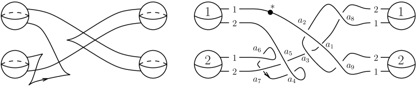
Figure 7. An oriented Legendrian knot in $\#^{2}(S^{1}\times S^{2})$: front in Gompf standard form (left), and resolution with base point $\ast$ (right).

The knot has $tb=1$ and $r=0$ (note that $tb$ is well-defined since the knot is null-homologous). The differential graded algebra $\mathcal{A}$ associated to the knot has generators $a_{1},\dots,a_{9},c_{12}^{0},\tilde{c}_{12}^{0}$, and $c_{ij}^{p},\tilde{c}_{ij}^{p}$ for $1\leq i,j\leq 2$ and $p\geq 1$, with grading

$$|a_{1}|=|a_{4}|=|a_{6}|=|a_{8}|=|a_{9}|=1,$$

$$|a_{2}|=|a_{3}|=|a_{5}|=|a_{7}|=|c_{12}^{0}|=|\tilde{c}_{12}^{0}|=0,$$

$$|c_{11}^{p}|=|\tilde{c}_{11}^{p}|=|c_{22}^{p}|=|\tilde{c}_{22}^{p}|=2p-1,$$

$$|c_{12}^{p}|=|\tilde{c}_{12}^{p}|=2p,$$

$$|c_{21}^{p}|=|\tilde{c}_{21}^{p}|=2p-2.$$

(Here for notational simplicity we have dropped the second subscript on $c_{ij;\ell}^{p}$ and instead write $c_{ij}^{p}:=c_{ij;1}^{p}$, $\tilde{c}_{ij}^{p}:=c_{ij;2}^{p}$.)

The differential on $\mathcal{A}$ is given by

$$\partial(a_{1}) =-a_{2}a_{3}+t^{-1}c_{12}^{0}a_{5} \partial(c_{12}^{0}) =\partial(\tilde{c}_{12}^{0})=0$$

$$\partial(a_{4}) =1+a_{5}a_{7} \partial(c_{21}^{1}) =\partial(\tilde{c}_{21}^{1})=0$$

$$\partial(a_{6}) =1+\tilde{c}_{12}^{0}a_{7} \partial(c_{11}^{1}) =1-c_{12}^{0}c_{21}^{1}$$

$$\partial(a_{8}) =-c_{12}^{0}+a_{3} \partial(\tilde{c}_{11}^{1}) =1-\tilde{c}_{12}^{0}\tilde{c}_{21}^{1}$$

$$\partial(a_{9}) =-\tilde{c}_{12}^{0}-a_{2} \partial(c_{22}^{1}) =1-c_{21}^{1}c_{12}^{0}$$

$$\partial(a_{i}) =0,~{}~{}~{}~{}i\neq 1,4,6,8,9 \partial(\tilde{c}_{22}^{1}) =1-\tilde{c}_{21}^{1}\tilde{c}_{12}^{0}$$

$$\partial(c_{12}^{1}) =-c_{12}^{0}c_{22}^{1}+c_{11}^{1}c_{12}^{0}$$

$$\partial(\tilde{c}_{12}^{1}) =-\tilde{c}_{12}^{0}\tilde{c}_{22}^{1}+\tilde{c}_{11}^{1}\tilde{c}_{12}^{0}$$

and so forth for the differentials of $c_{ij}^{p}$ and $\tilde{c}_{ij}^{p}$, $p\geq 2$.

We remark that $(\mathcal{A},\partial)$ has a graded augmentation over $\mathbb{Z}/2$ (and indeed over $\mathbb{Z}$ if we set $t=-1$), given by the graded algebra map $\epsilon:\thinspace\mathcal{A}\to\mathbb{Z}/2$ determined by $\epsilon(a_{2})=\epsilon(a_{3})=\epsilon(a_{5})=\epsilon(a_{7})=\epsilon(c_{12}^{0})=\epsilon(\tilde{c}_{12}^{0})=\epsilon(c_{21}^{1})=\epsilon(\tilde{c}_{21}^{1})=1$ and $\epsilon=0$ for all other generators of $\mathcal{A}$. It follows from the results of the subsequent section (see Corollary 2.21) that the Legendrian knot pictured in Figure 7 is not destabilizable.

2.6. Stable tame isomorphism for countably generated DGAs

In this section, we discuss the notion of equivalence of DGAs that we need in order to state the invariance result for the DGAs described in Section 2.4. For finitely generated semifree DGAs, this equivalence was first described by Chekanov [7], who called it “stable tame isomorphism”. We extend his notion here to countably generated semifree DGAs.

Definition 2.9.

Let $I$ be a countable index set, either $\{1,\ldots,n\}$ for some $n$ or $\mathbb{N}=\mathbb{Z}_{>0}$, and let $R$ be a commutative ring with unit. A semifree algebra over $R$ is an algebra $\mathcal{A}$ over $R$, along with a distinguished set of generators $\{a_{i}\,|\,i\in I\}\subset\mathcal{A}$, such that $\mathcal{A}$ is the unital tensor algebra over $R$ freely generated by the $\{a_{i}\}$:

$$\mathcal{A}=R\langle a_{1},a_{2},\ldots\rangle.$$

Thus $\mathcal{A}$ is freely generated as an $R$-module by finite-length words in the $a_{i}$, including the empty word. A semifree differential graded algebra $(\mathcal{A},\partial)$ over $R$ is a semifree algebra $\mathcal{A}$ over $R$, equipped with a grading (additive over products, with $R$ in grading $0$) and a degree $-1$ differential $\partial$ satisfying the signed Leibniz rule: $\partial(ab)=(\partial a)b+(-1)^{|a|}a(\partial b)$.

Note that the differential $\partial$ on a semifree DGA is determined by its values on the generators $a_{i}$, $i\in I$. In practice, $R$ will be either $\mathbb{Z}[\mathbf{t},\mathbf{t}^{-1}]$ or a quotient such as $\mathbb{Z}/2$.

We next define two classes of automorphisms of a semifree DGA, the elementary and the tame automorphisms. These do not involve the differential.

Definition 2.10.

An ordering of a semifree algebra $\mathcal{A}$ over $R$ is a bijection $\sigma\colon I\to I$, which we picture as giving an increasing total order of the generators of $\mathcal{A}$ by setting $a_{\sigma(1)}<a_{\sigma(2)}<a_{\sigma(3)}<\cdots$. Any ordering produces a filtration on $\mathcal{A}$,

$$R=\mathcal{F}^{0}\mathcal{A}\subset\mathcal{F}^{1}\mathcal{A}\subset\mathcal{F}^{2}\mathcal{A}\subset\cdots\subset\mathcal{A},$$

where $\mathcal{F}^{k}\mathcal{A}=R\langle a_{\sigma(1)},a_{\sigma(2)},\ldots,a_{\sigma(k)}\rangle$.

Definition 2.11.

Let $\mathcal{A}$ be a semifree algebra over $R$. An elementary automorphism of $\mathcal{A}$ is a grading-preserving algebra map $\phi:\thinspace\mathcal{A}\to\mathcal{A}$ such that there exists an ordering $\sigma$ of $\mathcal{A}$ for which for all $k\in I$,

$$\phi(a_{\sigma(k)})=u_{k}a_{\sigma(k)}+v_{k},$$

where $u_{k}$ is a unit in $R$ and $v_{k}\in\mathcal{F}^{k-1}\mathcal{A}$.

Informally, an elementary automorphism is a map that sends each generator $a_{k}$ to itself plus terms that are strictly lower in the ordering than $a_{k}$. Note that any elementary automorphism preserves the corresponding filtration $\{F^{k}\mathcal{A}\}$ of $\mathcal{A}$.

Remark 2.12.

The more familiar notion of an elementary automorphism in the sense of Chekanov [7] (which is defined when the index set $I$ is finite, but the notion can be extended to any index set) is also an elementary automorphism in the sense of Definition 2.11. For Chekanov (see also [17]), an algebra map $\phi:\thinspace\mathcal{A}\to\mathcal{A}$ is elementary automorphism if there exists an $i$ such that $\phi(a_{i})=ua_{i}+v$ for $u$ a unit and $v\in\mathcal{A}$ not involving $a_{i}$, and $\phi(a_{j})=a_{j}$ for all $j\neq i$. Given such a $\phi$, suppose the generators of $\mathcal{A}$ appearing in $v$ are $a_{j_{1}},\ldots,a_{j_{\ell}}$ where $j_{1},\ldots,j_{\ell}\neq i$. Then any ordering $\sigma$ satisfying $\sigma(1)=j_{1}$, …, $\sigma(\ell)=j_{\ell}$, $\sigma(\ell+1)=i$ fulfills the condition of Definition 2.11.

Conversely, an elementary automorphism $\phi$ as given in Definition 2.11 is a composition of Chekanov’s elementary automorphisms: for $k\in I$, define $\phi_{k}$ by $\phi_{k}(a_{\sigma(k)})=u_{k}a_{\sigma(k)}+v_{k}$ and $\phi_{k}(a_{j})=a_{j}$ for all $j\neq\sigma(k)$; then

$$\phi=\cdots\circ\phi_{3}\circ\phi_{2}\circ\phi_{1}.$$

Note that this composition is infinite if $I$ is infinite, but converges when applied to any element of $\mathcal{A}$.

From now on, the term “elementary automorphism” will be in the sense of Definition 2.11.

Proposition 2.13.

Any elementary automorphism of a semifree algebra is invertible, and its inverse is also an elementary automorphism.

Proof.

Suppose that $\phi$ is an elementary automorphism of $\mathcal{A}$ with ordering $\sigma$, units $u_{k}$, and algebra elements $v_{k}$ as in Definition 2.11. Note that $v_{1}\in\mathcal{F}^{0}\mathcal{A}=R$. Construct an algebra map $\psi\colon\mathcal{A}\to\mathcal{A}$ as follows. We define $\psi(a_{\sigma(k)})$ inductively on $k$ by:

$$\psi(a_{\sigma(1)}) =u_{1}^{-1}(a_{\sigma(1)}-v_{1}),$$

$$\psi(a_{\sigma(k)}) =u_{k}^{-1}(a_{\sigma(k)}-\psi(v_{k})).$$

Note that this is constructed so that $\psi(v_{k})\in\mathcal{F}^{k-1}\mathcal{A}$ and $\psi(a_{\sigma(k)})\in\mathcal{F}^{k}\mathcal{A}$ for all $k$, as is clear by induction. (In particular, $\psi(v_{k})$ is determined by $\psi(a_{\sigma(1)}),\ldots,\psi(a_{\sigma(k-1)})$.) It is straightforward to check by induction on $k$ that $\psi(\phi(a_{\sigma(k)}))=\phi(\psi(a_{\sigma(k)}))=a_{\sigma(k)}$, and so $\psi=\phi^{-1}$. ∎

Definition 2.14.

A tame automorphism of a semifree algebra is a composition of finitely many elementary automorphisms.

Note crucially that different elementary automorphisms may have different orderings associated to them: it is not the case that a tame automorphism must preserve one particular filtration of the algebra.

It follows from Proposition 2.13 that every tame automorphism is invertible, with another tame automorphism as its inverse. Thus the set of tame automorphisms forms a group, and the following relation is an equivalence relation.

Definition 2.15.

A tame isomorphism between two semifree differential graded algebras $(\mathcal{A},\partial)$ and $(\mathcal{A}^{\prime},\partial^{\prime})$, with generators $\{a_{i}\,|\,i\in I\}$ and $\{a_{i}^{\prime}\,|\,i\in I\}$ respectively for a common index set $I$, is a graded algebra map $\phi\colon\mathcal{A}\to\mathcal{A}^{\prime}$ with

$$\phi\circ\partial=\partial^{\prime}\circ\phi,$$

such that we can write $\phi=\phi_{2}\circ\phi_{1}$, where $\phi_{1}\colon\mathcal{A}\to\mathcal{A}$ is a tame automorphism and $\phi_{2}$ is the algebra map sending $a_{i}$ to $a_{\sigma(i)}^{\prime}$ for all $i\in I$, where $\sigma\colon I\to I$ is any bijection such that $|a_{i}|=|a_{\sigma(i)}^{\prime}|$ for all $i$. If there is a tame isomorphism between $(\mathcal{A},\partial)$ and $(\mathcal{A}^{\prime},\partial^{\prime})$, then the DGAs are tamely isomorphic.

The final ingredient in stable tame isomorphism is the notion of an algebraic stabilization of a DGA. Our definition of stabilization extends the corresponding definition in [7] by allowing countably many generators to be added simultaneously.

Definition 2.16.

Let $(\mathcal{A},\partial)$ be a semifree DGA over $R$ generated by $\{a_{i}\,|\,i\in I\}$. A stabilization of $(\mathcal{A},\partial)$ is a semifree DGA $(S(\mathcal{A}),\partial)$ constructed as follows. Let $J$ be a countable (possibly finite) index set. Then $S(\mathcal{A})$ is the tensor algebra over $R$ generated by $\{a_{i}\,|\,i\in I\}\cup\{e_{j}\,|\,j\in J\}\cup\{f_{j}\,|\,j\in J\}$, graded in such a way that the grading on the $a_{i}$ is inherited from $\mathcal{A}$, and $|e_{j}|=|f_{j}|+1$ for all $j\in J$. The differential on $S(\mathcal{A})$ agrees on $\mathcal{A}\subset S(\mathcal{A})$ with the original differential $\partial$, and is defined on the $e_{j}$ and $f_{j}$ by

$$\partial(e_{j})=f_{j},~{}~{}~{}~{}~{}~{}~{}~{}~{}~{}\partial(f_{j})=0$$

for all $j\in J$; extend to all of $S(\mathcal{A})$ by the Leibniz rule as usual.

Now we can define our notion of equivalence for countably generated DGAs.

Definition 2.17.

Two semifree DGAs $(\mathcal{A},\partial)$ and $(\mathcal{A}^{\prime},\partial^{\prime})$ are stable tame isomorphic if some stabilization of $(\mathcal{A},\partial)$ is tamely isomorphic to some stabilization of $(\mathcal{A}^{\prime},\partial^{\prime})$.

Note that stable tame isomorphism is an equivalence relation.

With this in hand, we can state the main algebraic invariance result for the DGA associated to a Legendrian link in $\#^{k}(S^{1}\times S^{2})$.

Theorem 2.18.

Let $\Lambda$ and $\Lambda^{\prime}$ be Legendrian links in $\#^{k}(S^{1}\times S^{2})$ in normal form, and suppose that $\Lambda$ and $\Lambda^{\prime}$ are Legendrian isotopic. Let $(\mathcal{A},\partial)$ and $(\mathcal{A}^{\prime},\partial^{\prime})$ be the semifree DGAs over $\mathbb{Z}[\mathbf{t},\mathbf{t}^{-1}]$ associated to the diagrams $\pi_{xy}(\Lambda)$ and $\pi_{xy}(\Lambda^{\prime})$, which are in $xy$-normal form. Then $(\mathcal{A},\partial)$ and $(\mathcal{A}^{\prime},\partial^{\prime})$ are stable tame isomorphic.

Theorem 2.18 will be proven in Section B.2. In practice, given a front projection for a Legendrian link in $\#^{k}(S^{1}\times S^{2})$ in Gompf standard form, one resolves it following the procedure in Section 2.2 and then computes the DGA associated to the resolved diagram; up to stable tame isomorphism, this DGA is an invariant of the original Legendrian link.

We conclude this section with some general algebraic remarks about stable tame isomorphism. First, just as for finitely generated DGAs, stable tame isomorphism is a special case of quasi-isomorphism.

Proposition 2.19.

If $(\mathcal{A},\partial)$ and $(\mathcal{A}^{\prime},\partial^{\prime})$ are stable tame isomorphic, then $H_{*}(\mathcal{A},\partial)\cong H_{*}(\mathcal{A}^{\prime},\partial^{\prime})$.

Proof.

This is essentially the same as the corresponding proof in [7], see also [17, Cor. 3.11]. If $(\mathcal{A},\partial)$ and $(\mathcal{A}^{\prime},\partial^{\prime})$ are tamely isomorphic, then they are chain isomorphic and the result follows. It suffices to check that if $(S(\mathcal{A}),\partial)$ is a stabilization of $(\mathcal{A},\partial)$, then the homologies are isomorphic. Let $\iota:\thinspace\mathcal{A}\to S(\mathcal{A})$ denote inclusion, and let $\pi:\thinspace S(\mathcal{A})\to\mathcal{A}$ denote the projection that sends any term involving an $e_{j}$ or $f_{j}$ to $0$. Then $\pi\circ\iota=Id_{\mathcal{A}}$. If we define $H:\thinspace S(\mathcal{A})\to S(\mathcal{A})$ by

$$H(v) =0 v\in\mathcal{A}$$

$$H(ve_{j}w) =0 v\in\mathcal{A},~{}w\in S(\mathcal{A})$$

$$H(vf_{j}w) =(-1)^{|v|+1}ve_{j}w v\in\mathcal{A},~{}w\in S(\mathcal{A}),$$

then it is straightforward to check that on $S(\mathcal{A})$,

$$H\circ\partial+\partial\circ H=\iota\circ\pi-Id_{S(\mathcal{A})}.$$

The result follows. ∎

Second, we can apply the usual machinery (augmentations, linearizations, the characteristic algebra [27], etc.) to semifree DGAs up to stable tame isomorphism. For now, we consider augmentations.

Definition 2.20.

A graded augmentation (over $\mathbb{Z}/2$) of a semifree DGA $(\mathcal{A},\partial)$ is a graded algebra map $\epsilon:\thinspace\mathcal{A}\to\mathbb{Z}/2$, where $\mathbb{Z}/2$ lies in degree $0$, for which $\epsilon\circ\partial=0$.

Corollary 2.21.

The existence or nonexistence of a graded augmentation of $(\mathcal{A},\partial)$ is invariant under Legendrian isotopy.

As in [7], if $\Lambda$ is a (geometric) stabilization of another Legendrian link $\Lambda^{\prime}$, then the differential graded algebra for $\Lambda$ is trivial up to stable tame isomorphism, and in particular has no graded augmentations.

Corollary 2.22.

If $(\mathcal{A},\partial)$ has a graded augmentation, then $\Lambda$ is not destabilizable.

Figure 8. A Legendrian link passing exactly once through a $1$-handle is Legendrian isotopic to its double stabilization. The second move is Gompf move 6 (see Figure 23); the others are planar Legendrian isotopies.

Remark 2.23.

Suppose that the Legendrian link $\Lambda$ passes through any of the $1$-handles exactly once ($n_{j}=1$ for some $j$). Then it is easy to check that $(\mathcal{A},\partial)$ is trivial, because $\partial c_{11;j}^{1}=1$. Indeed, it is the case that any such $\Lambda$ is Legendrian isotopic to its own double stabilization (i.e., the result of stabilizing $\Lambda$ once positively and once negatively); see Figure 8.

We can repeat this argument to conclude that $\Lambda$ is Legendrian isotopic to arbitrarily high double stabilizations of itself. It follows that the Legendrian isotopy class of such a link is determined by its formal Legendrian isotopy class (topological class and rotation number).

A Legendrian link in $\#^{k}(S^{1}\times S^{2})$ passing through some handle once could be considered an imprecise analogue of a loose Legendrian knot in an overtwisted contact $3$-manifold, i.e., a Legendrian knot whose complement is overtwisted (see [16]), in the sense that both of these are infinitely destabilizable. It is also reminiscent of a loose Legendrian embedding in higher dimensions [23].

3. Calculations and applications

In this section, we present a number of calculations of Legendrian contact homology in connected sums of $S^{1}\times S^{2}$, as well as some applications, notably a new proof of the existence of exotic Stein structures on $\mathbb{R}^{8}$.

3.1. The cotangent bundle of $T^{2}$

Consider the Legendrian knot $\Lambda_{1}\subset\#^{2}(S^{1}\times S^{2})$ from Section 2.5. As shown in [19], handle attachment along this knot yields a Stein structure on the $D^{2}$-bundle over $T^{2}$ with Euler number $0$, that is, $DT^{*}T^{2}$; see also Proposition 3.5. We will explicitly calculate the Legendrian contact homology in this case.

The DGA for $\Lambda_{1}$ was computed in Section 2.5. Recall from there that it has a differential subalgebra, the internal DGA, generated by internal Reeb chords $c_{ij}^{p},\tilde{c}_{ij}^{p}$.

Proposition 3.1.

The differential graded algebra for $\Lambda_{1}$ is stable tame isomorphic to the internal DGA along with one additional generator, $a$, of degree $1$, whose differential is

$$\partial(a)=c_{12}^{0}\tilde{c}_{12}^{0}+t\tilde{c}_{12}^{0}c_{12}^{0}.$$

Proof.

Beginning with the differential graded algebra for $\Lambda_{1}$ from Section 2.5, we successively apply the tame automorphisms $a_{2}\mapsto a_{2}-\tilde{c}_{12}^{0}$, $a_{3}\mapsto a_{3}+c_{12}^{0}$, $a_{1}\mapsto a_{1}+a_{9}a_{3}+\tilde{c}_{12}^{0}a_{8}+a_{9}c_{12}^{0}$; the resulting differential has

$$\partial(a_{1}) =\tilde{c}_{12}^{0}c_{12}^{0}+t^{-1}c_{12}^{0}a_{5}$$

$$\partial(a_{4}) =1+a_{5}a_{7}$$

$$\partial(a_{6}) =1+\tilde{c}_{12}^{0}a_{7}$$

$$\partial(a_{8}) =a_{3}$$

$$\partial(a_{9}) =-a_{2}.$$

Destabilize to eliminate the generators $a_{2},a_{3},a_{8},a_{9}$, and then successively apply the tame automorphisms $a_{4}\mapsto a_{4}+a_{5}(\tilde{c}_{22}^{1}a_{7}+\tilde{c}_{21}^{1}a_{6})$, $a_{1}\mapsto t^{-1}a_{1}+t^{-1}c_{12}^{0}(-a_{4}\tilde{c}_{12}^{0}+a_{5}\tilde{c}_{22}^{1})$, $a_{4}\mapsto a_{4}+\tilde{c}_{11}^{1}$, $a_{5}\mapsto a_{5}+\tilde{c}_{12}^{0}$, $a_{6}\mapsto a_{6}+\tilde{c}_{11}^{1}$, $a_{7}\mapsto a_{7}-\tilde{c}_{21}^{1}$. This gives

$$\partial(a_{1}) =c_{12}^{0}\tilde{c}_{12}^{0}+t\tilde{c}_{12}^{0}c_{12}^{0}$$

$$\partial(a_{4}) =-a_{5}\tilde{c}_{21}^{1}$$

$$\partial(a_{6}) =\tilde{c}_{12}^{0}a_{7}.$$

To complete the proof, we need to eliminate $a_{4},a_{5},a_{6},a_{7}$; this is done in the lemma that follows, with $(v,w,x,y)=(\tilde{c}_{11}^{1},\tilde{c}_{22}^{1},\tilde{c}_{12}^{0},\tilde{c}_{21}^{1})$ allowing us to eliminate $(a,b)=(a_{4},a_{5})$ and $(a,b)=(a_{6},a_{7})$ in turn. ∎

Lemma 3.2.

Let $(\mathcal{A},\partial)$ be a differential graded algebra whose generators include $v,w,x,y$ with $|v|=|w|=1$, $|x|=|y|=0$,

$$\partial(x)=\partial(y)=0,~{}~{}~{}~{}~{}\partial(v)=1-xy,~{}~{}~{}~{}~{}\partial(w)=1-yx.$$

Let $(\mathcal{A}^{\prime},\partial)$ be the differential graded algebra given by appending two generators $a,b$ to the generators of $\mathcal{A}$, with $|a|=|b|+1$ and differential given by the differential on $\mathcal{A}$, along with $\partial(b)=0$ and $\partial(a)$ equal to one of the following:

$$\partial(a)=\pm xb,\pm bx,\pm yb,\pm by.$$

Then $(\mathcal{A}^{\prime},\partial)$ is stable tame isomorphic to $(\mathcal{A},\partial)$.

Proof.

We will prove the lemma when $\partial(a)=xb$; the other cases are clearly similar. Stabilize $(\mathcal{A}^{\prime},\partial)$ once by adding $e_{11},e_{12}$ with $|e_{11}|=|e_{12}|+1=|a|+1$ and $\partial(e_{11})=e_{12},\partial(e_{12})=0$. Applying the successive elementary automorphisms $e_{12}\mapsto e_{12}-ya-wb$, $e_{11}\mapsto e_{11}+we_{12}$, $a\mapsto a+xe_{12}$ yields

$$\partial(e_{11})=-ya,~{}\partial(e_{12})=b,~{}\partial(a)=\partial(b)=0.$$

Destabilize once by removing $e_{12},b$, and stabilize once by adding $e_{21},e_{22}$ with $|e_{21}|=|e_{22}|+1=|a|+2$ and $\partial(e_{21})=e_{22},\partial(e_{22})=0$. Applying the successive elementary automorphisms $e_{22}\mapsto e_{22}+xe_{11}-va$, $e_{21}\mapsto e_{21}+ve_{22}$, $e_{11}\mapsto e_{11}-ye_{22}$ yields

$$\partial(e_{21})=xe_{11},~{}\partial(e_{22})=a,~{}\partial(a)=\partial(e_{11})=0.$$

Finally, destabilize once by removing $e_{22},a$ to obtain an algebra generated by the generators of $\mathcal{A}$ along with $e_{21},e_{11}$ with $|e_{21}|=|e_{11}|+1=|a|+2$ and $\partial(e_{21})=xe_{11},\partial(e_{11})=0$.

This procedure shows that $\mathcal{A}^{\prime}$ is stable tame isomorphic to the same algebra but with the gradings of $a,b$ both increased by $2$, and if we omit $a,b$, then the resulting algebra is $\mathcal{A}$. We can then iterate the procedure, adding generators to $\mathcal{A}^{\prime}$ in successively higher grading, to conclude the following. Let $(S(\mathcal{A}^{\prime}),\partial)$ be the stabilization of $(\mathcal{A}^{\prime},\partial)$ obtained by adding $e_{i1},e_{i2}$ for all $i\geq 1$, with $|e_{i1}|=|e_{i2}|+1=|a|+i$ and $\partial(e_{i1})=e_{i2}$, $\partial(e_{i2})=0$. Then $(S(\mathcal{A}^{\prime}),\partial)$ is tamely isomorphic to $(S(\mathcal{A}^{\prime}),\partial^{\prime})$, where $\partial^{\prime}$ is the same differential as $\partial$ except

$$\partial^{\prime}(e_{12}) =b, \partial^{\prime}(b) =0,$$

$$\partial^{\prime}(e_{22}) =a, \partial^{\prime}(a) =0,$$

$$\partial^{\prime}(e_{i+2,2}) =e_{i1}, \partial^{\prime}(e_{i1}) =0, i \geq 1.$$

But $(S(\mathcal{A}^{\prime}),\partial^{\prime})$ is a stabilization of $(\mathcal{A},\partial)$, and the lemma is proven. ∎

From Proposition 3.1, we can calculate the Legendrian contact homology of $\Lambda_{1}$ in degree $0$, which is $H_{0}(\mathcal{A},\partial)$ where $(\mathcal{A},\partial)$ is the DGA for $\Lambda_{1}$. In particular, we have the following result.

Proposition 3.3.

If we set $t=-1$, then the Legendrian contact homology of $\Lambda_{1}$ in degree $0$ is

$$\mathbb{Z}[x_{1}^{\pm 1},x_{2}^{\pm 1}]\cong\mathbb{Z}[\pi_{1}(T^{2})].$$

Proof.

By Proposition 3.1, we want to calculate $H_{0}(\mathcal{A},\partial)$ where $(\mathcal{A},\partial)$ is the internal DGA along with $a$. Since $\mathcal{A}$ is supported in nonnegative degree, the subalgebra in degree $0$, which is generated by $c_{12}^{0},c_{21}^{1},\tilde{c}_{12}^{0},\tilde{c}_{21}^{1}$, consists entirely of cycles. The boundaries in degree $0$ are generated by the differentials of generators of degree $1$: $\partial(a)=c_{12}^{0}\tilde{c}_{12}^{0}-\tilde{c}_{12}^{0}c_{12}^{0}$, $\partial(c_{11}^{1})=1-c_{12}^{0}c_{21}^{1}$, $\partial(c_{22}^{1})=1-c_{21}^{1}c_{12}^{0}$, $\partial(\tilde{c}_{11}^{1})=1-\tilde{c}_{12}^{0}\tilde{c}_{21}^{1}$, $\partial(\tilde{c}_{22}^{1})=1-\tilde{c}_{21}^{1}\tilde{c}_{12}^{0}$. Thus in homology, $c_{21}^{1}$ and $\tilde{c}_{21}^{1}$ are the multiplicative inverses of $c_{12}^{0}$ and $\tilde{c}_{12}^{0}$ respectively. If we write $c_{12}^{0}=x_{1}$ and $\tilde{c}_{12}^{0}=x_{2}$, then in homology, $\partial(a)$ causes $x_{1}$ and $x_{2}$ to commute, and thus $H_{0}(\mathcal{A},\partial)\cong\mathbb{Z}[x_{1}^{\pm 1},x_{2}^{\pm 1}]$, as desired. ∎

Remark 3.4.

It can be shown that the entire Legendrian contact homology of $\Lambda_{1}$, $H_{*}(\mathcal{A},\partial)$, is supported in degree $0$, but we omit the proof here.

From the point of view of the symplectic homology of $T^{\ast}T^{2}$, the Legendrian DGA is isomorphic to the (twisted) linearized contact homology of the co-core disk of the surgery, see [5, Section 5.4]. This linearized contact homology is isomorphic to the wrapped Floer homology of the co-core disk (i.e. the fiber in $T^{\ast}T^{2}$), see e.g. [15, Proof of Theorem 7.2]. The wrapped homology of the fiber is in turn is isomorphic to the homology of the based loop space of $T^{2}$, see [1, 2], which is $\mathbb{Z}[\pi_{1}(T^{2})]$ in agreement with our calculation.

We also point out that the fact that we need to take $t=-1$ in Proposition 3.3 corresponds to changing our choice of the Lie group spin structure on the knot in defining the signs to the bounding spin structure which extends over the core disk of the handle as is required in the construction of the surgery isomorphism.

3.2. The cotangent bundle of $\Sigma_{g}$

This is a generalization of the previous example. Let $\Lambda_{1}$ be the Legendrian knot in $\#^{2}(S^{1}\times S^{2})$ given in the previous section, and let $\Lambda_{2}$ be the knot in $\#^{4}(S^{1}\times S^{2})$ drawn in Figure 9. This construction generalizes to $\Lambda_{g}\subset\#^{2g}(S^{1}\times S^{2})$ for any $g\geq 1$. It can readily be calculated that $\Lambda_{g}$ is nullhomologous and has Thurston–Bennequin number $2g-1$ and rotation number $0$.

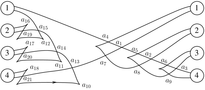
Figure 9. The Legendrian knot $\Lambda_{2}\subset\#^{4}(S^{1}\times S^{2})$.

The significance of $\Lambda_{g}$ is contained in the following result.

Proposition 3.5.

Handle attachment along $\Lambda_{g}$ gives a Stein structure on $DT^{*}\Sigma_{g}$, the disk cotangent bundle of the Riemann surface of genus $g$.

2pt 1 at 50 144 2 at 15 109 3 at 15 55 4 at 50 19 1 at 105 19 2 at 140 55 3 at 140 109 4 at 105 144 1 at 253 149 2 at 253 104 3 at 253 59 4 at 253 14 1 at 424 149 2 at 424 104 3 at 424 59 4 at 424 14

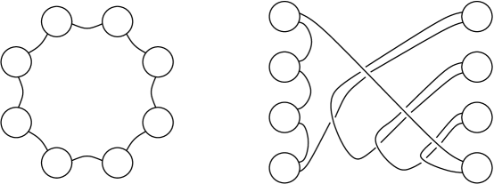
Figure 10. Obtaining a disk bundle over $\Sigma_{2}$ by handle attachment.

Proof.

We restrict ourselves to the case $g=2$ (the general case is similar), and follow [19]. A (slightly unorthodox) handle decomposition of a disk bundle over $\Sigma_{2}$ is given by the left diagram in Figure 10. Here the circles represent spheres, identified in pairs via reflection, and the arcs represent a knot in $\#^{4}(S^{1}\times S^{2})$ along which a $2$-handle is attached. Via isotopy, we may draw this handle decomposition in more standard form as the right diagram in Figure 9, where the spheres are now identified pairwise through reflection in a vertical plane. The Legendrian knot $\Lambda_{2}$ is simply a Legendrian form of the knot in Figure 9; note that it wraps around itself near the left spheres labeled $2,3,4$, but this does not change the isotopy class of the knot.

The particular disk bundle over $\Sigma_{2}$ determined by handle attachment along $\Lambda_{2}$ has Euler number given by $tb(\Lambda_{2})-1=2g-2$. This agrees with the Euler number of $DT^{*}\Sigma_{2}$, and the proposition follows. ∎

We now calculate the Legendrian contact homology of $\Lambda_{g}$. As in the previous section, the differential graded algebra for $\Lambda_{g}$ has an internal subalgebra generated by $2g$ copies of $(\mathcal{A}_{2},\partial_{2})$.

Proposition 3.6.

The differential graded algebra for $\Lambda_{g}$ is stable tame isomorphic to the internal subalgebra with one additional generator $a$ of degree $1$ whose differential is

$$\partial(a)=c_{12;2g}^{0}c_{12;2g-1}^{0}\cdots c_{12;2}^{0}c_{12;1}^{0}+tc_{12;1}^{0}c_{12;2}^{0}\cdots c_{12;2g-1}^{0}c_{12;2g}^{0}.$$

Proof.

We will assume $g=2$; the general case is similar. Label crossings in the resolution of $\Lambda_{2}$ as follows: the crossings corresponding to front crossings and right cusps are labeled in Figure 9; there are four additional crossings $d_{1},d_{2},d_{3},d_{4}$, corresponding to the half-twists at the right of the diagram for handles $1$, $2$, $3$, $4$. Pick a base point along the strand of $\Lambda_{2}$ connecting crossing $a_{4}$ leftwards to handle $1$. The non-internal differential is given by

$$\partial(a_{1}) =-a_{4}a_{7}+t^{-1}c_{12;1}^{0}a_{15}a_{14}a_{13} \partial(a_{16}) =1+c_{12;2}^{0}a_{19}$$

$$\partial(a_{2}) =-a_{4}-a_{5}a_{8} \partial(a_{17}) =1+c_{12;3}^{0}a_{20}$$

$$\partial(a_{3}) =-a_{5}-a_{6}a_{9} \partial(a_{18}) =1+c_{12;4}^{0}a_{21}$$

$$\partial(a_{10}) =1+a_{13}a_{21} \partial(d_{1}) =a_{7}-c_{12;1}^{0}$$

$$\partial(a_{11}) =1+a_{14}a_{20} \partial(d_{2}) =a_{8}-c_{12;2}^{0}$$

$$\partial(a_{12}) =1+a_{15}a_{19} \partial(d_{3}) =a_{9}-c_{12;3}^{0}$$

$$\partial(d_{4}) =-a_{6}-c_{12;4}^{0}$$

and the differential of all other non-internal generators is $0$.

Applying the tame automorphism

$$a_{1} \mapsto a_{1}+a_{2}a_{7}-a_{3}a_{8}a_{7}+d_{4}a_{9}a_{8}a_{7}+c_{12;4}^{0}d_{3}a_{8}a_{7}+c_{12;4}^{0}c_{12;3}^{0}d_{2}a_{7}$$

$$\qquad+c_{12;4}^{0}c_{12;3}^{0}c_{12;2}^{0}d_{1}$$

yields $\partial(a_{1})=c_{12;4}^{0}c_{12;3}^{0}c_{12;2}^{0}c_{12;1}^{0}+t^{-1}c_{12;1}^{0}a_{15}a_{14}a_{13}$. Next define the auxiliary quantities $g_{2},g_{3},g_{4},h_{2},h_{3},h_{4}$ by

$$g_{2} =c_{21;2}^{1}a_{16}+c_{22;2}^{1}a_{19} h_{2} =-a_{12}c_{12;2}^{0}+a_{15}g_{2}c_{12;2}^{0}+a_{15}c_{22;2}^{1}$$

$$g_{3} =c_{21;3}^{1}a_{17}+c_{22;3}^{1}a_{20} h_{3} =-a_{11}c_{12;3}^{0}+a_{14}g_{3}c_{12;3}^{0}+a_{14}c_{22;3}^{1}$$

$$g_{4} =c_{21;4}^{1}a_{18}+c_{22;4}^{1}a_{21} h_{4} =-a_{10}c_{12;4}^{0}+a_{13}g_{4}c_{12;4}^{0}+a_{13}c_{22;4}^{1},$$

and note that $\partial(g_{2})=a_{19}+c_{21;2}^{1}$, $\partial(g_{3})=a_{20}+c_{21;3}^{1}$, $\partial(g_{4})=a_{21}+c_{21;4}^{1}$, $\partial(h_{2})=a_{15}-c_{12;2}^{0}$, $\partial(h_{3})=a_{14}-c_{12;3}^{0}$, $\partial(h_{4})=a_{13}-c_{12;4}^{0}$. Thus applying the tame automorphism

$$a_{1}\mapsto t^{-1}(a_{1}+c_{12;1}^{0}h_{2}a_{14}a_{13}+c_{12;1}^{0}c_{12;2}^{0}h_{3}a_{13}+c_{12;1}^{0}c_{12;2}^{0}c_{12;3}^{0}h_{4})$$

now gives $\partial(a_{1})=tc_{12;4}^{0}c_{12;3}^{0}c_{12;2}^{0}c_{12;1}^{0}+c_{12;1}^{0}c_{12;2}^{0}c_{12;3}^{0}c_{12;4}^{0}$.

Next, the succession of tame automorphisms $a_{4}\mapsto-a_{4}-a_{5}a_{8}$, $a_{5}\mapsto-a_{5}-a_{6}a_{9}$, $a_{6}\mapsto a_{6}-c_{12;4}^{0}$, $a_{7}\mapsto a_{7}+c_{12;1}^{0}$, $a_{8}\mapsto a_{8}+c_{12;2}^{0}$, $a_{9}\mapsto a_{9}+c_{12;3}^{0}$ gives

$$\partial(a_{2})=a_{4},~{}\partial(a_{3})=a_{5},~{}\partial(d_{1})=a_{7},~{}\partial(d_{2})=a_{8},~{}\partial(d_{3})=a_{9},~{}\partial(d_{4})=a_{6},$$

and we can destabilize to eliminate the generators $a_{2},\ldots,a_{9},d_{1},d_{2},d_{3},d_{4}$. Finally, apply the successive tame automorphisms $a_{10}\mapsto a_{10}+a_{13}g_{4}+c_{11;4}^{1}$, $a_{11}\mapsto a_{11}+a_{14}g_{3}+c_{11;3}^{1}$, $a_{12}\mapsto a_{12}+a_{15}g_{2}+c_{11;2}^{1}$, $a_{16}\mapsto a_{16}+c_{11;2}^{1}$, $a_{17}\mapsto a_{17}+c_{11;3}^{1}$, $a_{18}\mapsto a_{18}+c_{11;4}^{1}$, $a_{13}\mapsto a_{13}+c_{12;4}^{0}$, $a_{14}\mapsto a_{14}+c_{12;3}^{0}$, $a_{15}\mapsto a_{15}+c_{12;2}^{0}$, $a_{19}\mapsto a_{19}-c_{21;2}^{1}$, $a_{20}\mapsto a_{20}-c_{21;3}^{1}$, $a_{21}\mapsto a_{21}-c_{21;4}^{1}$ to get

$$\partial(a_{10}) =a_{13}c_{21;4}^{1} \partial(a_{16}) =c_{12;2}^{0}a_{19}$$

$$\partial(a_{11}) =a_{14}c_{21;3}^{1} \partial(a_{17}) =c_{12;3}^{0}a_{20}$$

$$\partial(a_{12}) =a_{15}c_{21;2}^{1} \partial(a_{18}) =c_{12;4}^{0}a_{21},$$

and we can eliminate $a_{10},\ldots,a_{21}$ by Lemma 3.2. What remains is the internal subalgebra and $a_{1}$. ∎

Proposition 3.7.

If we set $t=-1$, then the Legendrian contact homology of $\Lambda_{g}$ in degree $0$ is

$$\mathbb{Z}\langle x_{1}^{\pm 1},x_{2}^{\pm 1},\ldots,x_{2g}^{\pm 1}\rangle\,/\,(x_{1}x_{2}\cdots x_{2g}-x_{2g}\cdots x_{2}x_{1})\cong\mathbb{Z}[\pi_{1}(\Sigma_{g})].$$

Proof.

Nearly identical to the proof of Proposition 3.3. In this case, the identification is given by $c_{12;\ell}^{0}\mapsto x_{\ell}$, $c_{21;\ell}^{1}\mapsto x_{\ell}^{-1}$ for $1\leq\ell\leq 2g$, and the differential $\partial(a)$ gives the desired relation $x_{1}x_{2}\cdots x_{2g}=x_{2g}\cdots x_{2}x_{1}$ in homology. ∎

Remark 3.8.

As was the case for $\Lambda_{1}$, it can be shown that the entire Legendrian contact homology of $\Lambda_{g}$ is supported in degree $0$. Also, as there our calculation can be interpreted as a calculation of the wrapped Floer homology of a fiber in $T^{\ast}\Sigma_{g}$ which is isomorphic to the homology of the based loop space, i.e. $\mathbb{Z}[\pi_{1}(\Sigma_{g})]$.

3.3. Exotic Stein structure on $\mathbb{R}^{8}$

Let $\Lambda$ be the Legendrian knot in $S^{1}\times S^{2}$ depicted in Figure 11. Note that $\Lambda$ generates $H_{1}(S^{1}\times S^{2})$, i.e., it winds algebraically once around $S^{1}$. This means in particular that the Weinstein $4$-manifold $W$ that results from adding a $2$-handle along $\Lambda$ is contractible (although its fundamental group at infinity is nontrivial).

We will prove the following result.

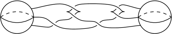
Figure 11. The Legendrian knot $\Lambda\subset S^{1}\times S^{2}$.

Proposition 3.9.

The Legendrian contact homology of $\Lambda$, i.e., the homology of $(\mathcal{A}(\Lambda),\partial(\Lambda))$, is nonzero.

Before proving Proposition 3.9, we deduce a result about exotic Stein structures on $\mathbb{R}^{8}$. Let $W$ be the Weinstein $4$-manifold given by attaching a $2$-handle to $S^{1}\times D^{3}$ along $\Lambda$. Then the product $W\times W$ inherits a Stein structure from $W$.

Proposition 3.10.

$W\times W$ is diffeomorphic to $\mathbb{R}^{8}$ but the Stein structure on $W\times W$ is distinct from the standard Stein structure on $\mathbb{R}^{8}$.

Proof.

First note that $W$ is contractible. Consider the boundary of $W\times W$ as the result of joining the bundles $W\times\partial W$ and $\partial W\times W$ along their common boundary $\partial W\times\partial W$. Note that any loop in the boundary of $W\times W$ is homotopic to a loop in $\partial W\times\partial W$, which is null-homotopic since $W$ is contractible. Thus we find that $\partial(W\times W)$ is a homotopy $7$-sphere that bounds the contractible manifold $W\times W$. It follows that $W\times W$ is in fact diffeomorphic to $\mathbb{R}^{8}$.

It remains to show that the Stein structure on $W\times W$ is not the standard one on $\mathbb{R}^{8}$. By Proposition 3.9, for the Legendrian homology DGA $(\mathcal{A}(\Lambda),\partial(\Lambda))$, the unit $1\in\mathcal{A}(\Lambda)$ is not in the image of the differential $\partial(\Lambda)$. It follows it follows that the homology of the Hochschild complex $A^{\rm Ho}(\Lambda)$ is nonzero, and thus from [5] that the symplectic homology $SH(W)$ is nonzero. Now the Künneth formula in symplectic homology [28] gives

$$SH(W\times W)\cong SH(W)\otimes SH(W)\neq 0=SH(\mathbb{R}^{8}),$$

and we conclude that $W\times W$ is an exotic Stein $\mathbb{R}^{8}$. ∎

Remark 3.11.

The same result holds for any Legendrian knot $\Lambda\subset S^{1}\times S^{2}$ that generates $H_{1}(S^{1}\times S^{2})$ and has nonzero Legendrian contact homology. A “simpler” example of such a $\Lambda$ is given in Remark 3.12; see Figure 13.

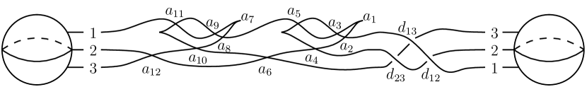
Figure 12. A knot Legendrian isotopic to $\Lambda$, with half-twist added and $xy$-projection crossings labeled.

Proof of Proposition 3.9.

For the purposes of this result, it suffices to work over the ring $\mathbb{Z}/2$ instead of $\mathbb{Z}[t,t^{-1}]$ by setting $t=1$ and reducing mod $2$. We will show that the homology for the DGA over this ring has a certain quotient that has (somewhat remarkably) previously appeared in the literature on Legendrian contact homology in a rather different context [31].

For computational convenience, change $\Lambda$ by a Legendrian isotopy by pulling out two of its cusps, to give the knot in Figure 12; this causes all holomorphic disks (besides those in the internal differential) to be embedded rather than just immersed. The non-internal differential for the knot shown in Figure 12 is

$$\partial(a_{1}) =1+a_{5}a_{4}+(1+a_{9}a_{11})a_{6}+a_{9}c_{12}^{0}$$

$$\partial(a_{2}) =(1+a_{3}a_{5})a_{4}+a_{3}(1+a_{9}a_{11})a_{6}+a_{3}a_{9}c_{12}^{0}$$

$$\partial(a_{7}) =1+a_{11}a_{10}+c_{12}^{0}a_{12}+c_{13}^{0}$$

$$\partial(a_{8}) =(1+a_{9}a_{11})a_{10}+a_{9}c_{12}^{0}a_{12}+a_{9}c_{13}^{0}$$

$$\partial(a_{12}) =c_{23}^{0}$$

$$\partial(d_{12}) =c_{12}^{0}+1+a_{3}a_{5}$$

$$\partial(d_{13}) =c_{13}^{0}+d_{12}c_{23}^{0}+(1+a_{3}a_{5})d_{23}+a_{3}(1+a_{9}a_{11}),$$

with zero differential for all other non-internal generators.

Let $\mathcal{A}^{\prime}=(\mathbb{Z}/2)\langle a,b,c,d\rangle$ be the tensor algebra on four generators $a,b,c,d$. Define an algebra map $\phi:\thinspace\mathcal{A}\to\mathcal{A}^{\prime}$ by

$$\phi(c_{12}^{0})=a,~{}\phi(c_{13}^{0})=d,~{}\phi(c_{21}^{1})=c,~{}\phi(c_{31}^{1})=b,$$

$$\phi(a_{3})=1,~{}\phi(a_{4})=1,~{}\phi(a_{5})=a+1,~{}\phi(a_{9})=1,~{}\phi(a_{10})=1,~{}\phi(a_{11})=d+1,$$

and $\phi=0$ for all other generators of $\mathcal{A}$. It is straightforward to check that $\phi\circ\partial=0$ on all non-internal generators of $\mathcal{A}$. On internal generators of $\mathcal{A}$, we have

$$(\phi\circ\partial)(c_{32}^{1}) =ba,$$

$$(\phi\circ\partial)(c_{11}^{1}) =1+ac+db,$$

$$(\phi\circ\partial)(c_{22}^{1}) =1+ca,$$

$$(\phi\circ\partial)(c_{33}^{1}) =1+bd,$$

$$(\phi\circ\partial)(c_{23}^{1}) =cd,$$

and $(\phi\circ\partial)(c_{ij}^{p})=0$ for all other internal generators.

It follows that $\phi$ induces a surjective algebra map from $\mathcal{A}$ to the quotient

$$\mathcal{A}^{\prime\prime}=(\mathbb{Z}/2)\langle a,b,c,d\rangle/(1+ac+db,1+ca,1+bd,ba,cd),$$

and this is a chain map from $(\mathcal{A},\partial)$ to $(\mathcal{A}^{\prime\prime},0)$. Thus $\phi$ descends to a surjection from $H(\mathcal{A},\partial)$ to $\mathcal{A}^{\prime\prime}$. But it was proven in [31] that $\mathcal{A}^{\prime\prime}$ is nonzero. ∎

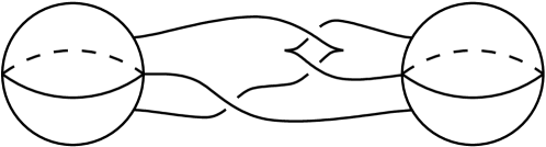
Figure 13. Another Legendrian knot in $S^{1}\times S^{2}$.

Remark 3.12.

It can also be shown that the Legendrian knot shown in Figure 13, which is slightly simpler than $\Lambda$ but also winds homologically once around $S^{1}$, also has nonzero Legendrian contact homology. Thus this knot also produces an exotic Stein structure on $\mathbb{R}^{8}$. However, the proof that the homology is nonzero in this case appears to be more complicated than the proof of Proposition 3.9; the proof known to us uses Gröbner bases calculated via computational algebra software.

4. Geometric constructions for relating the combinatorial invariant to Legendrian homology

4.1. Main result and overview of Sections 4 and 5

As mentioned in Section 1, the Legendrian contact homology (Legendrian homology, for short) of a Legendrian link $\Lambda$ is a part of SFT and is in particular defined using moduli spaces of holomorphic disks. We will discuss this theory in the setting relevant to this paper in Section 5 below. Here we just describe its basic structure for Legendrian links $\Lambda\subset Y_{k}=\#^{k}(S^{1}\times S^{2})$. Legendrian homology associates a DGA $\mathcal{A}_{\mathrm{H}}(\Lambda)$ with differential $\partial_{\mathrm{H}}$ to $\Lambda$. The algebra $\mathcal{A}_{\mathrm{H}}(\Lambda)$ is freely generated by the Reeb chords of $\Lambda$ over $\mathbb{Z}[\mathbf{t},\mathbf{t}^{-1}]$ and the differential $\partial_{\mathrm{H}}$ is defined through a count of holomorphic disks in the symplectization $\mathbb{R}\times Y_{k}$ with Lagrangian boundary condition $\mathbb{R}\times\Lambda$. The main result of the paper can then be stated as follows:

Theorem 4.1.

The Legendrian homology DGA $\mathcal{A}_{\mathrm{H}}(\Lambda)$ of a link $\Lambda\subset Y_{k}$ in Gompf normal form is canonically isomorphic to the combinatorially defined algebra $\mathcal{A}$ associated to $\Lambda$ in Section 2.4. The canonical isomorphism is a one-to-one map that takes Reeb chords to generators of $\mathcal{A}$ and that intertwines the differentials $\partial_{\mathrm{H}}$ on $\mathcal{A}_{\mathrm{H}}$ and $\partial$ on $\mathcal{A}$.

The proof of Theorem 4.1 is rather involved and occupies Sections 4 and 5. Before we outline its steps we comment on the definition of $\mathcal{A}_{\mathrm{H}}(\Lambda)$. The algebra $\mathcal{A}_{\mathrm{H}}(\Lambda)$ depends on the choice of contact form on $Y_{k}$, and below we will equip $Y_{k}$ with contact forms that depend on positive parameters $(\epsilon,\delta)$. The set of Reeb chords of $\Lambda$ will in the present setup (unlike in the case of ambient contact manifold $\mathbb{R}^{3}$) not be finite. In general Legendrian homology algebras come equipped with natural action filtrations and are defined as corresponding direct limits. For the contact form on $Y_{k}$ that we use below the action is related to the grading of the algebra, which simplifies the situation somewhat. Theorem 4.1 should be interpreted as follows. For any given degree there exists $(\epsilon_{0},\delta_{0})$ such that for $Y_{k}$ equipped with the contact form corresponding to $(\epsilon,\delta)$ with $\epsilon<\epsilon_{0}$ and $\delta<\delta_{0}$, the natural map in the formulation has the properties stated on the part of the algebra of action less than the given degree, and furthermore, the homology of $\mathcal{A}$ is canonically isomorphic to the homology of $\mathcal{A}_{\mathrm{H}}$ defined via the action filtration.

The proof of Theorem 4.1 involves a study of holomorphic disks in specific contact models of $Y_{k}$ and associated contact and symplectic manifolds. We study aspects of the geometric constructions and properties of these models in this section, followed by holomorphic disks in Section 5.

4.2. Contact and symplectic pairs

In this section we consider constructions of pairs $(Y,\Lambda)$ where $Y$ is a contact $3$-manifold and $\Lambda$ is a Legendrian link, as well as pairs $(X,L)$, where $X$ is a Weinstein $4$-manifold and $L$ an exact Lagrangian submanifold in $X$ with cylindrical ends, i.e., outside a compact subset $(X,L)$ looks like a disjoint union of half symplectizations of contact pairs $(Y,\Lambda)$.

4.2.A. One-handles

Consider ${\mathbb{C}}^{2}$ with coordinates $(z_{1},z_{2})=(x_{1}+iy_{1},x_{2}+iy_{2})$. For $\delta>0$, consider the region

$$H_{\delta}=\left\{(z_{1},z_{2})\colon-\delta^{2}\leq\tfrac{1}{2}\left(x_{1}^{2}+y_{1}^{2}\right)+2x^{2}_{2}-y_{2}^{2}\leq\delta^{2}\right\}$$

with boundary given by the hypersurfaces

$$V_{\pm\delta}=\left\{(z_{1},z_{2})\colon\tfrac{1}{2}\left(x_{1}^{2}+y_{1}^{2}\right)+2x^{2}_{2}-y_{2}^{2}=\pm\delta^{2}\right\}.$$

Topologically, $V_{-\delta}\approx_{\rm top}\mathbb{R}^{3}\times S^{0}$ and $V_{\delta}\approx_{\rm top}S^{2}\times\mathbb{R}$. The normal vector field

(4.1) $$Z=\tfrac{1}{2}\left(x_{1}\,\partial_{x_{1}}+y_{1}\,\partial_{y_{1}}\right)+2x_{2}\,\partial_{x_{2}}-y_{2}\,\partial_{y_{2}}$$

of $V_{\pm\delta}$ is a Liouville vector field of the standard symplectic form $\omega_{\rm st}$ on ${\mathbb{C}}^{2}$, where

$$\omega_{\rm st}=dx_{1}\wedge dy_{1}+dx_{2}\wedge dy_{2}.$$

That is, if $L$ denotes the Lie-derivative then

$$L_{\!Z}\,\omega_{\rm st}=d(\omega(Z,\cdot))=d\left(\tfrac{1}{2}(x_{1}\,dy_{1}-y_{1}\,dx_{1})+2x_{2}\,dy_{2}+y_{2}\,dx_{2}\right)=\omega_{\rm st}.$$

Note that $Z$ points out of $H_{\delta}$ along $V_{\delta}$ and into $H_{\delta}$ along $V_{-\delta}$.

The Liouville vector field $Z$ determines the contact forms $\alpha_{\pm\delta}$ along $V_{\pm\delta}$ where

$$\alpha_{\pm\delta}=\omega_{\rm st}(Z,\cdot)|_{V_{\pm\delta}}=\left.\left(\tfrac{1}{2}(x_{1}\,dy_{1}-y_{1}\,dx_{1})+2x_{2}\,dy_{2}+y_{2}\,dx_{2}\right)\right|_{V_{\pm\delta}}.$$

Trivializations of the contact structures $\operatorname{ker}(\alpha_{\pm\delta})$ are given by $(v,iv)$, where

(4.2) $$v=2x_{2}\,\partial_{x_{1}}+y_{2}\,\partial_{y_{1}}-\tfrac{1}{2}(x_{1}\,\partial_{x_{2}}-y_{1}\,\partial_{y_{2}})$$

and $i$ denotes the complex structure on ${\mathbb{C}}^{2}$. The Reeb vector field $R$ of $\alpha_{\pm\delta}$ satisfies $R=N\tilde{R}$, where

(4.3) $$\tilde{R}=\left.\left(\tfrac{1}{2}(x_{1}\,\partial_{y_{1}}-y_{1}\,\partial_{x_{1}})+2x_{2}\,\partial_{y_{1}}+y_{2}\,\partial_{x_{2}}\right)\right|_{V_{\pm\delta}},$$

and where the normalization factor $N$ is given by

$$N=\left(\tfrac{1}{4}\left(x_{1}^{2}+y_{1}^{2}\right)+4x_{2}^{2}+y_{2}^{2}\right)^{-1}.$$

The flow lines of the Reeb flow are thus the solution curves of the following system of ordinary differential equations

$$\begin{cases}\dot{x}_{1}=-\tfrac{1}{2}y_{1},\\ \dot{y}_{1}=\tfrac{1}{2}x_{1},\\ \dot{x}_{2}=y_{2},\\ \dot{y}_{2}=2x_{2},\end{cases}$$

given by

(4.4) $$x_{1}(t) =x_{1}(0)\,\cos\left(\tfrac{1}{2}t\right)+y_{1}(0)\,\sin\left(\tfrac{1}{2}t\right),$$

(4.5) $$y_{1}(t) =-x_{1}(0)\,\sin\left(\tfrac{1}{2}t\right)+y_{1}(0)\,\cos\left(\tfrac{1}{2}t\right),$$

(4.6) $$x_{2}(t) =x_{2}(0)\,\cosh\left(\sqrt{2}\,t\right)+\tfrac{1}{\sqrt{2}}y_{2}(0)\,\sinh\left(\sqrt{2}\,t\right),$$

(4.7) $$y_{2}(t) =\sqrt{2}x_{2}(0)\,\sinh\left(\sqrt{2}\,t\right)+y_{2}(0)\,\cosh\left(\sqrt{2}\,t\right),$$

where $(x_{1}(0)+iy_{1}(0),x_{2}(0)+iy_{2}(0))$ is the initial position.

Lemma 4.2.

There is exactly one geometric closed Reeb orbit $\gamma$ in $V_{\delta}$. If $\gamma^{m}$ denotes the $m^{\rm th}$ iterate of $\gamma$ then

$$\operatorname{CZ}(\gamma^{m})=2m,$$

where $\operatorname{CZ}$ denotes the Conley–Zehnder index measured with respect to the trivialization $(v,iv)$, see (4.2).

Proof.

The statement on the uniqueness of the geometric orbit is immediate from the explicit expression for the Reeb flow lines above. In the trivialization on the contact planes along $\gamma$ given by $(\partial_{x_{2}},\partial_{y_{2}})$ the linearized Reeb flow is given by Equations (4.6) and (4.7). A straightforward calculation shows that the Conley–Zehnder index of the corresponding path of matrices equals $0$. The frame $(\partial_{x_{2}},\partial_{y_{2}})$ makes one full turn in the positive direction with respect to the frame $(v,iv)$ per iterate of $\gamma$. It follows that $\operatorname{CZ}(\gamma^{m})=2m$. ∎

The standard Legendrian strand in $V_{\delta}$ is the subset

$$\Lambda_{\rm st}=\left\{(x_{1},y_{1},x_{2},y_{2})\in V_{\delta}\colon y_{1}=x_{2}=0\right\}.$$

Lemma 4.3.

The Reeb chords of $\Lambda_{\rm st}\subset V_{\delta}$ are exactly the Reeb orbits $\gamma^{k}$ and the image under the linearized Reeb flow of the tangent space to $\Lambda_{\rm st}$ at the initial point of the chord is transverse to the tangent space at its end point.

Proof.

Immediate from the expression for the Reeb flow lines above. ∎

4.2.B. Standard contact $\mathbb{R}^{3}$ and standard contact balls

The standard contact form on $\mathbb{R}^{3}$ is the $1$-form

$$\alpha_{\rm st}=dz-y\,dx,$$

where $(x,y,z)$ are coordinates on $\mathbb{R}^{3}=J^{1}(\mathbb{R})$ with $x$ a coordinate on $\mathbb{R}$, $z$ the coordinate of function values in $J^{0}(\mathbb{R})$, and $y$ the fiber coordinate in $T^{\ast}\mathbb{R}$.

We define the standard contact ball of radius $\rho>0$ as the subset

$$B_{\rho} =\left\{(u,v,z)\in\mathbb{R}^{3}\colon u^{2}+v^{2}+z^{2}\leq\rho^{2}\right\}$$

$$=\left\{(r,\theta,z)\in\mathbb{R}_{+}\times S^{1}\times\mathbb{R}\colon r^{2}+z^{2}\leq\rho^{2}\right\},$$

with the contact form

$$\alpha_{\rm b}=dz+\tfrac{1}{2}(u\,dv-v\,du)=dz-\tfrac{1}{2}r^{2}\,d\theta,$$

where $(r,\theta)$ are polar coordinates on the $uv$-plane.

Let $p=(x_{0},y_{0},z_{0})\in\mathbb{R}^{3}$ and consider the embedding $F\colon B_{\rho}\to\mathbb{R}^{3}$

(4.8) $$F(u,v,z)=(u+x_{0}\,,\,v+y_{0}\,,\,z+z_{0}+y_{0}u+\tfrac{1}{2}uv).$$

Note that $F$ is a contact embedding, i.e., $F^{\ast}\alpha_{\rm st}=\alpha_{\rm b}$. We call $F(B_{\rho})$ the standard contact ball of radius $\rho$ centered at $p$.

4.2.C. The manifold $Y_{k}(\delta)$, standard $\mathbb{R}^{3}$ with $k$ 1-handles

The contact manifold $Y_{k}(\delta)$ is topologically $\mathbb{R}^{3}$ with $2k$ balls removed and $k$ 1-handles (i.e. $[-1,1]\times S^{2}$) attached along the boundaries of the removed balls.

We first describe the attaching loci for the handles. Fix $2k$ points

$$\left\{\left(0,y^{\ell},z^{\ell}\right)\,,\,\left(A,\tilde{y}^{\ell},\tilde{z}^{\ell}\right)\right\}_{1\leq\ell\leq k}$$

in $\mathbb{R}^{3}$ as in Section 2.1. Let $\sigma$ denote the minimal distance between two of these points and fix standard contact balls, see Section 4.2.B, of radii $\rho\ll\sigma$ centered at these points. These balls will be the attaching locus. Let $\mathbb{R}^{3}_{\rho}(\circ_{k})$ denote the complement of the standard contact balls of radius $\rho/2$ centered at these points.

We then consider identifications of regions near the boundary of the standard contact balls centered at two corresponding points

$$p^{-}=\left(0,y^{\ell},z^{\ell}\right)\quad\text{and}\quad p^{+}=\left(A,\tilde{y}^{\ell},\tilde{z}^{\ell}\right)$$

with two regions in the standard handle, see Section 4.2.A, that will be used for the handle attachment. Fix $\delta\ll\rho$ and consider the two regions

(4.9) $$\begin{split}A_{\rho}^{+}(\delta)&=\left\{(x_{1},y_{1},x_{2},y_{2})\in V_{-\delta}\colon x_{2}=0,y_{2}>0,x_{1}^{2}+y_{1}^{2}\leq\rho^{2}\right\},\\ A_{\rho}^{-}(\delta)&=\left\{(x_{1},y_{1},x_{2},y_{2})\in V_{-\delta}\colon x_{2}=0,y_{2}<0,x_{1}^{2}+y_{1}^{2}\leq\rho^{2}\right\},\end{split}$$

see Figure 14, and the map $G\colon A_{\rho}^{\pm}(\delta)\to B_{\rho}$, where $B_{\rho}$ is the standard contact ball:

(4.10) $$G(x_{1},y_{1},0,y_{2})=(x_{1},y_{1},0).$$

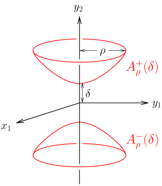
Figure 14. The regions $A_{\rho}^{\pm}(\delta)\subset V_{-\delta}$.

Then

$$G^{\ast}\left(dz+\tfrac{1}{2}(u\,dv-v\,du)\right)=\tfrac{1}{2}(x_{1}\,dy_{1}-y_{1}\,dx_{1}).$$

Thus $G^{\ast}\alpha_{\rm b}=\alpha_{-\delta}|_{A_{\rho}^{\pm}(\delta)}$. The Reeb vector fields of $\alpha_{-\delta}$ and $\alpha_{\rm b}$ are transverse to $A_{\rho}^{\pm}(\delta)$ respectively $G(A_{\rho}^{\pm}(\delta))$ and we use their flows to construct a contactomorphism from a neighborhood of $A_{\rho}^{\pm}(\delta)$ to $B_{\rho}$. We use the notation $B_{\rho}^{\pm}(\delta)\subset V_{-\delta}$ for this neighborhood of $A_{\rho}^{\pm}(\delta)$, see Figure 15. Thus $B^{\pm}_{\rho}(\delta)$ is identified with a neighborhood of $p^{\pm}$.

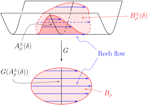
Figure 15. The regions $B_{\rho}^{\pm}(\delta)\subset V_{-\delta}$.

We use the flow of the Liouville vector field $Z$, see (4.1), to identify $B_{\rho}^{\pm}(\delta)-B_{\rho/2}^{\pm}(\delta)\subset V_{-\delta}$ with a region in $V_{\delta}$. More precisely, let $\Phi^{t}_{Z}\colon\mathbb{R}^{4}\to\mathbb{R}^{4}$ denote the time $t$ flow generated by the vector field $Z$. Then for each $p\in B_{\rho}^{\pm}(\delta)-B_{\rho/2}^{\pm}(\delta)$ there is a unique time $T(p)$ such that $\Phi_{Z}^{T(p)}(p)\in V_{\delta}$ and we define the map

$$\phi\colon\bigl{(}B_{\rho}^{+}(\delta)-B_{\rho/2}^{+}(\delta)\bigr{)}\cup\bigl{(}B_{\rho}^{-}(\delta)-B_{\rho/2}^{-}(\delta)\bigr{)}\to V_{\delta},\quad\phi(p)=\Phi_{Z}^{T(p)}(p).$$

Then $\phi^{\ast}\alpha_{\delta}=e^{T}\alpha_{-\delta}$. See Figure 16.

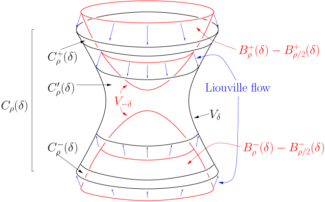
Figure 16. The map $\phi$ identifies regions in $V_{\pm\delta}$ via the Liouville flow.

We next estimate the function $T$ and its derivative. The time $t$ flow of $Z$ with initial condition $p=(x_{1}(0),y_{1}(0),x_{2}(0),y_{2}(0))$ is given by

$$\Phi_{Z}^{t}(p)=\left(e^{\tfrac{1}{2}t}x_{1}(0)\,,\,e^{\tfrac{1}{2}t}y_{1}(0)\,,\,e^{2t}x_{2}(0)\,,\,e^{-t}y_{2}(0)\right).$$

Thus the function $T=T(p)$ solves the equation

$$\frac{1}{2}e^{T}\left(x_{1}(0)^{2}+y_{1}(0)^{2}\right)+e^{4T}2x_{2}(0)^{2}-e^{-2T}y_{2}(0)^{2}=\delta^{2}.$$

Using the fact that the initial value lies in $B_{\rho}(\delta)-B_{\rho/2}(\delta)\subset V_{-\delta}$, we can rewrite this as

(4.11) $$\begin{split}\delta^{2}&=\frac{1}{2}\left(e^{T}-e^{-2T}\right)\left(x_{1}(0)^{2}+y_{1}(0)^{2}\right)+2\left(e^{4T}-e^{-2T}\right)x_{2}(0)^{2}-\delta^{2}e^{-2T}\\ &=\frac{e^{T}}{2}\left(x_{1}(0)^{2}+y_{1}(0)^{2}\right)+2e^{4T}x_{2}(0)^{2}-e^{-2T}\left(\delta^{2}+\frac{1}{2}\left(x_{1}(0)^{2}+y_{1}(0)^{2}\right)+2x_{2}(0)^{2}\right).\\ \end{split}$$

Noting that all coefficient functions (functions that depend on $T$) in the final line of (LABEL:eq:defneqnT) are increasing in $T$, we deduce first that

$$T={\mathbf{O}}(\delta^{2}/\rho^{2})$$

and second that the solution $T$ decreases monotonically with the quantity $\left(x_{1}(0)^{2}+y_{1}(0)^{2}+x_{2}(0)^{2}\right)$ and hence that the differential of $T$ satisfies

$$|dT|={\mathbf{O}}(\delta^{2}/\rho^{3}).$$

Let $C_{\rho}(\delta)\subset V_{\delta}$ be the region with boundary $\phi(\partial B_{\rho}^{+}(\delta)\cup\partial B_{\rho}^{-}(\delta))$ which contains $\phi\left(B_{\rho}^{\pm}(\delta)-B_{\rho/2}^{\pm}(\delta)\right)$, let $C_{\rho}^{\prime}(\delta)\subset V_{\delta}$ be the region with boundary $\phi\left(\partial B_{\rho/2}^{+}(\delta)\cup B_{\rho/2}^{-}(\delta)\right)$ which does not contain $\phi\left(B_{\rho}^{\pm}(\delta)-B_{\rho/2}^{\pm}(\delta)\right)$, and let $C^{\pm}_{\rho}(\delta)=\phi\left(B_{\rho}^{\pm}(\delta)-B_{7\rho/8}^{\pm}(\delta)\right)$. See Figure 16.

Let $\alpha_{\rho;\delta}$ denote the contact form on $C_{\rho}(\delta)$ given by

$$\alpha_{\rho;\delta}=e^{f}\alpha_{\delta},$$

where $f\colon C_{\rho}(\delta)\to\mathbb{R}$ has the following properties:

• $f=-T\circ\phi^{-1}$ on $C^{\pm}_{\rho}(\delta)$;

• $f=0$ on $C_{\rho}^{\prime}(\delta)$;

• $|df|={\mathbf{O}}(\delta^{2}/\rho^{3})$.

The above estimates on $T$ show that such a function $f$ exists. Then

$$\phi\colon(B_{\rho}^{\pm}(\delta)-B_{7\rho/8}^{\pm}(\delta),\alpha_{-\delta})\to(C_{\rho}^{\pm}(\delta),\alpha_{\rho;\delta})$$

is a contactomorphism.

Finally, as discussed above, we consider $B^{\pm}_{\rho}(\delta)$ as neighborhoods of $p^{\pm}$ in $\mathbb{R}^{3}$, and then define $Y_{k}(\delta)$ as the contact manifold

$$Y_{k}(\delta)=\mathbb{R}^{3}_{\rho}(\circ_{k})\,\,\,\bigcup_{\phi}\,\,\,\left(\sqcup_{\ell=1}^{k}C_{\rho}^{\ell}(\delta)\right),$$

where $C^{\ell}_{\rho}(\delta)$ is a copy of $C_{\rho}(\delta)$ attached via the map $\phi$ at the pair of points $\left(0,y^{\ell},z^{\ell}\right)$ and $\left(A,\tilde{y}^{\ell},\tilde{z}^{\ell}\right)$. We denote the contact form on $Y_{k}(\delta)$ by $\alpha_{k;\delta}$.

Lemma 4.4.

For all sufficiently small $\delta>0$, there are exactly $k$ distinct geometric Reeb orbits $\gamma_{1},\dots,\gamma_{k}$ in $Y_{k}(\delta)$, one in each handle. Furthermore if $\gamma_{j}^{m}$ denotes the $m^{\rm th}$ iterate of $\gamma_{j}$ then

$$\operatorname{CZ}(\gamma^{m}_{j})=2m,$$

where $\operatorname{CZ}$ denotes the Conley–Zehnder index measured with respect to the trivialization $(v,iv)$ as in (4.2).

Proof.

Since the $C^{1}$-distance between the contact forms $\alpha_{\delta}$ and $\alpha_{\rho;\delta}$ on $C_{\rho}(\delta)$ is controlled by $\delta$, the lemma is an immediate consequence of Lemma 4.2. ∎

Choose $R>0$ such that $B_{R/2}$ contains all the balls $B_{\rho}$ where the $1$-handles of $Y_{k}(\delta)$ are attached. (The factor of $2$ is not used here but will be used in Section 4.2.E.) Then $\mathbb{R}^{3}-B_{R}\subset Y_{k}(\delta)$, and we write

(4.12) $$\overline{Y}_{k}(\delta)=Y_{k}(\delta)-\operatorname{int}(\mathbb{R}^{3}-B_{R}).$$

Then the contact form $\alpha_{k;\delta}$ on $\overline{Y}_{k}(\delta)$ agrees with $\alpha_{\rm b}$ in a neighborhood of $\partial\overline{Y}_{k}(\delta)$ which is identified with a neighborhood of $\partial B_{R}$ in $B_{R}$.

4.2.D. Legendrian links in $Y_{k}(\delta)$

Let $\Lambda\subset Y_{k}(\delta)$ be any Legendrian link. Then there exists a contact isotopy which moves $\Lambda$ to a link in normal form, see Section 2.2. Below, all our links will be assumed to be in normal form. With notation as in Section 2.4 we have the following result.

Lemma 4.5.

Any Reeb chord of a link $\Lambda$ in normal form is either entirely contained in the handle and then of the form $c^{p}_{ij}$ or it lies completely in the complement of all handles.

Proof.

It is straightforward to check that no Reeb chord can connect a point on $\Lambda$ inside a handle to a point outside the handle (compare Section 5.3.C). The last statement follows from the fact that inside the handles $\Lambda$ is the graph of the differential of a function on the standard strand in a small $1$-jet neighborhood of that strand in combination with Lemma 4.3. ∎

We call Reeb chords of the first type mentioned in Lemma 4.5 handle chords and those of the second type diagram chords.

4.2.E. The closed manifold $\tilde{Y}_{k}(\epsilon;\delta)$

Consider the hypersurface

$$E(a):=\left\{(z_{1},z_{2})\in{\mathbb{C}}^{2}\colon|z_{1}|^{2}+a^{-1}|z_{2}|^{2}=1\right\}.$$

The vector field

$$W=\frac{1}{2}\left(x_{1}\partial_{x_{1}}+y_{1}\partial_{y_{1}}+x_{2}\partial_{x_{2}}+y_{2}\partial_{y_{2}}\right)$$

is a Liouville vector field for $\omega_{\rm st}$. Since $W$ is transverse to $E(a)$ it induces a contact form

$$\alpha_{a}=\omega(W,\cdot)=\left(x_{1}\,dy_{1}-y_{1}\,dx_{1}+x_{2}\,dy_{2}-y_{2}\,dx_{2}\right)|_{E(a)}.$$

The corresponding contact structure is isotopic to the standard contact structure on $S^{3}=E(1)$. The Reeb vector field on $E(a)$ is

$$R_{a}=(x_{1}\partial_{y_{1}}-y_{1}\partial_{x_{1}})+a^{-1}(x_{2}\partial_{y_{2}}-y_{2}\partial_{x_{2}}).$$

2pt $E(a)$ [tr] at 57 37 $F$ [l] at 329 93 $B_{\epsilon}(a)$ [b] at 220 182 $z_{2}=0$ [r] at 31 134 $z_{1}=0$ [b] at 180 208 $B_{d}$ [r] at 259 31

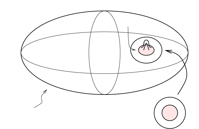
Figure 17. Constructing $\tilde{Y}_{k}(\epsilon;\delta)$; $1$-handles are attached in a small ball that does not intersect the two closed Reeb orbits.

Let $F\colon B_{d}\to E(a)$ be a contact embedding of a standard ball of radius $d$ such that $F(B_{d})$ does not intersect any complex coordinate plane. For $\epsilon>0$ sufficiently small, let $B_{\epsilon}(a)\subset E(a)$ denote the image under $F$ of the standard ball of radius $\epsilon$ centered at $0\in B_{d}$. See Figure 17.

Lemma 4.6.

If $a$ is irrational then the closed Reeb orbits in $E(a)$ are exactly the multiples of the two circles $E(a)\cap({\mathbb{C}}\times\{0\})$ and $E(a)\cap(\{0\}\times{\mathbb{C}})$. Furthermore, if the Liouville–Roth exponent of $a$ equals $p>2$ then there is a constant $K>0$ such that the following holds for all sufficiently small $\epsilon>0$. If $\gamma(t)$ is a Reeb trajectory which leaves $B_{\epsilon}$ at $t=0$ and if $T>0$ is such that $\gamma(T)\in B_{\epsilon}$, then $T\geq K\epsilon^{-\frac{1}{p}}$.

Proof.

The lemma is a consequence of the fact that outside the periodic orbits the Reeb flow is an irrational rotation on a torus with slope $a$: an orbit which returns to $B_{\epsilon}$ gives a rational approximation of $a$ of the form $\left|a-\frac{n}{m}\right|<\epsilon$. But then, by definition of the Liouville–Roth exponent, $\epsilon>m^{-p}$, for all sufficiently small $\epsilon$, and the action of $\gamma$ is bounded below by $Km$ for some $K$. ∎

Consider the map $\psi_{\epsilon}\colon B_{R}\to B_{\epsilon}$ defined by

$$\psi_{\epsilon}(u,v,z)=\left(\tfrac{\epsilon}{R}\,u,\tfrac{\epsilon}{R}\,v,\left(\tfrac{\epsilon}{R}\right)^{2}z\right)$$

and note that $\psi_{\epsilon}^{\ast}\alpha_{{\rm b}}=\left(\frac{\epsilon}{R}\right)^{2}\alpha_{\rm b}$. Since $\overline{Y}_{k}(\delta)$ agrees with $B_{R}$ near its boundary, see (4.12), we use the map $F\circ\psi_{\epsilon}$ in a neighborhood of the boundary to attach $\left(\overline{Y}_{k}(\delta),\left(\frac{\epsilon}{R}\right)^{2}\alpha_{k;\delta}\right)$ to $E(a)-B_{\epsilon}$. We denote the resulting contact manifold $\tilde{Y}_{k}(\epsilon;\delta)$ and its contact form $\tilde{\alpha}_{\epsilon;\delta}$.

Let $\Lambda\subset\overline{Y}_{k}(\delta)$ be a Legendrian link. Using the inclusion $\left(\overline{Y}_{k}(\delta),\left(\frac{\epsilon}{R}\right)^{2}\alpha_{k;\delta}\right)\to\left(\tilde{Y}_{k}(\epsilon;\delta),\tilde{\alpha}_{\epsilon;\delta}\right)$, we consider $\Lambda$ as a Legendrian link in $\tilde{Y}_{k}(\epsilon;\delta)$ and as such denote it $\Lambda(\epsilon)$.

Corollary 4.7.

If the Liouville–Roth exponent of $a\notin{\mathbb{Q}}$ equals $p>2$ then there is a constant $K>0$ such that the following holds for all sufficiently small $\epsilon>0$. If $c$ is a Reeb chord of $\Lambda(\epsilon)\subset\tilde{Y}_{k}(\epsilon;\delta)$ which is not entirely contained in $\overline{Y}_{k}(\delta)\subset\tilde{Y}_{k}(\epsilon)$ or if it is a Reeb orbit which is not a Reeb orbit in $E(a)$ then

$$\int_{c}\tilde{\alpha}_{\epsilon;\delta}\geq K\epsilon^{-\frac{1}{p}}.$$

Proof.

Immediate from Lemma 4.6. ∎

4.2.F. Exact cobordisms $(W_{k}(h;\delta),L(h))$

Let $\Lambda\subset\overline{Y}_{k}(\delta)$ be a Legendrian link. As above we consider $\Lambda$ as a link in $\tilde{Y}_{k}(\epsilon;\delta)$ and as such we denote it $\Lambda(\epsilon)$. For suitable positive functions $h\colon\mathbb{R}\to\mathbb{R}$ which are constantly equal to $\epsilon_{\pm}$ in a neighborhood of $\pm\infty$ we construct a symplectic cobordism $(W_{k}(h;\delta),L_{k}(h))$ with positive and negative ends $\left(\tilde{Y}_{k}(\epsilon_{+};\delta),\Lambda(\epsilon_{+})\right)$ and $\left(\tilde{Y}_{k}(\epsilon_{-};\delta),\Lambda(\epsilon_{-})\right)$, respectively. Topologically these cobordisms will simply be products $\mathbb{R}\times\tilde{Y}_{k}(\epsilon;\delta)$, but the symplectic form will not be the symplectization of a contact form. We construct them as follows.

Consider the standard contact ball $B_{d}$ of radius $d$ embedded into $E(a)$ and let $0<\epsilon_{\pm}\ll d$. We use strictly positive smooth functions $h\colon\mathbb{R}\to\mathbb{R}$ which satisfy the following conditions:

• There are $T_{-}<0<T_{+}$ such that

  (4.13) $$h(t)=\begin{cases}\epsilon_{-}&\text{if }t\in(-\infty,T_{-}],\\ \epsilon_{+}&\text{if }t\in[T_{+},\infty).\end{cases}$$

• The derivative of $h$ satisfies

  (4.14) $$2h^{\prime}(t)+h(t)>0.$$

Let $B_{d}(h)$ denote the manifold

$$B_{d}(h)=\left\{(t,p)\in\mathbb{R}\times B_{d}\colon|p|\geq\frac{1}{2}h(t)\right\}\approx_{\rm top}\mathbb{R}\times(B_{d}-B_{\epsilon_{-}}).$$

Endow $B_{d}(h)$ with the exact symplectic form $d\left(e^{t}\alpha_{\rm b}\right)$. Recall that we consider $B_{d}$ as embedded in $E(a)$ and define $\tilde{B}_{d}(h)\subset\mathbb{R}\times E(a)$ as follows:

$$\tilde{B}_{d}(h)=(\mathbb{R}\times(E(a)-B_{d}))\,\,\cup\,\,B_{d}(h).$$

Then the primitive $e^{t}\alpha_{\rm b}$ of the symplectic form on $B_{d}(h)$ extends as $e^{t}\alpha_{a}$ to $\mathbb{R}\times(E(a)-B_{d})$. Using this extension we consider also $\tilde{B}_{d}(h)$ as an exact symplectic manifold and we denote the primitive of its symplectic form $e^{t}\tilde{\alpha}$.

Consider the region $A$ in $\overline{Y}_{k}(\delta)$ outside the boundary of the standard contact ball of radius $\frac{R}{2}$:

$$A=B_{R}-B_{R/2}\subset\overline{Y}_{k}(\delta),$$

see (4.12). The map

$$\Phi\colon\mathbb{R}\times A\to B_{d}(h),\quad\Phi(t,q)=\left(t,h(t)u,h(t)v,h^{2}(t)z\right)$$

is a level preserving embedding such that

$$\Phi^{\ast}\left(e^{t}\alpha_{\rm b}\right)=\left(e^{t}h^{2}(t)\right)\alpha_{k;\delta}.$$

(Note that $h$ is increasing so that $|h(t)|\ll d$ for all $t\in\mathbb{R}$ and the image of $\Phi$ lies inside $B_{d}$.) We define the exact symplectic cobordism $W_{k}(h)$ as follows:

(4.15) $$W_{k}(h)=\left(\tilde{B}_{d}(h),e^{t}\alpha\right)\,\,\cup_{\Phi}\,\,\left(\mathbb{R}\times\overline{Y}_{k}(\delta),\left(e^{t}h^{2}(t)\right)\alpha_{k;\delta}\right),$$

where $\Phi$ is the gluing map. We must check that the form $d\left(e^{t}h^{2}(t)\alpha_{k;\delta}\right)$ on $\mathbb{R}\times\overline{Y}_{k}(\delta)$ is symplectic. We have

(4.16) $$d\left(e^{t}h^{2}(t)\alpha_{k;\delta}\right)=e^{t}h^{2}(t)\,d\alpha_{k;\delta}+e^{t}h(t)\left(2h^{\prime}(t)+h(t)\right)\,dt\wedge\alpha_{k;\delta}$$

and (4.14) implies that this is indeed symplectic.

Inside this symplectic cobordism we also have an exact Lagrangian cobordism $L(h)$ interpolating between the Legendrian submanifolds $\Lambda(\epsilon_{+})$ and $\Lambda(\epsilon_{-})$:

$$L(h)=\mathbb{R}\times\Lambda\subset\mathbb{R}\times\overline{Y}_{k}\subset W_{k}(h).$$

To see that $L(h)$ is Lagrangian, note that its tangent space is spanned by the tangent vector of $\Lambda$ and $\partial_{t}$. The vanishing of the restriction of the symplectic form then follows immediately from (4.16) in combination with $\Lambda$ being Legendrian.

Finally, we note that in the regions near $t=-\infty$ and $t=+\infty$ in (4.13) where $h(t)$ is constant, $\left(W_{k}(h),L(h)\right)$ is symplectomorphic to the symplectizations of $\left(\tilde{Y}_{k}(\epsilon_{-};\delta),\Lambda(\epsilon_{-})\right)$ and $\left(\tilde{Y}_{k}(\epsilon_{+};\delta),\Lambda(\epsilon_{+})\right)$, respectively.

5. Legendrian homology in closed and open manifolds

In this section we study the analytical aspects of Theorem 4.1, and in particular obtain rather explicit descriptions in Section 5.2 of the moduli spaces of holomorphic disks involved. In Section 5.3 we then study the actual solution spaces, and in Section 5.4 their orientation. However, before going into the detailed aspects of this study, we give in Section 5.1 a more general overview of Legendrian (contact) homology in order to provide a wider context of the more technical study that follows.

5.1. Legendrian homology in the ideal boundary of a Weinstein manifold

Our discussion in this section follows [5]. Let $Y$ be a contact manifold which is the ideal boundary of a Weinstein manifold $X$ with vanishing first Chern class $c_{1}(X)=0$. Pick an almost complex structure $J$ on $X$ which is compatible with the symplectic form and which in the end $[0,\infty)\times Y$ of $X$ splits as a complex structure in the contact planes of $Y$ and pairs the $\mathbb{R}$-direction $\partial_{t}$ with the Reeb vector field $R$ of the contact form on $Y$, $J\partial_{t}=R$. In this setup holomorphic curves satisfy SFT-compactness [4]: any finite energy holomorphic curve in $X$ is punctured and is asymptotic to a Reeb orbit cylinder $\mathbb{R}\times\gamma\subset\mathbb{R}\times Y$ at infinity. Furthermore, any sequence of holomorphic curves converges to a several-level holomorphic building with one level in $X$ and several levels in $\mathbb{R}\times Y$, where levels are joined at Reeb orbits.

Let $\Lambda\subset Y$ be a Legendrian submanifold. The Legendrian homology algebra $\mathcal{A}_{\mathrm{H}}(Y,\Lambda)$ is the algebra freely generated over $\mathbb{Z}[H_{2}(X,\Lambda)]$ by the set of Reeb chords of $\Lambda$ graded by a Maslov index, see [5, Section 2.1]. The differential in $\mathcal{A}_{\mathrm{H}}(Y,\Lambda)$ satisfies the Leibniz rule and is defined through a count of so-called anchored holomorphic disks. These are two-level holomorphic buildings of the following form. The top level is a map $u\colon(D,\partial D)\to(\mathbb{R}\times Y,\mathbb{R}\times\Lambda)$, where $D$ is a disk with the following punctures: one positive boundary puncture near which $u$ is asymptotic to $\mathbb{R}\times a$ for some Reeb chord $a$ of $\Lambda$, several negative boundary punctures where $u$ is asymptotic to $\mathbb{R}\times b$ for some Reeb chord $b$ of $\Lambda$ (possibly different for different punctures), and interior negative punctures where $u$ is asymptotic to $\mathbb{R}\times\gamma$ for some Reeb orbit $\gamma$ (again possibly different for different punctures). The lower level consists of holomorphic spheres with positive punctures at the Reeb orbits of all interior negative punctures of $u$. We write ${\mathcal{M}}_{A}^{(\mathbb{R}\times Y;X)}$ for the moduli space of such buildings, where $A$ denotes the homology class of the building. The differential acting on a Reeb chord $a$ is now defined as follows:

$$\partial_{\mathrm{H}}a=\sum_{\dim({\mathcal{M}}_{A}^{(\mathbb{R}\times Y;X)}(a;\mathbf{b}))=1}|{\mathcal{M}}_{A}^{(\mathbb{R}\times Y;X)}(a;\mathbf{b})|\,A\mathbf{b},$$

where $|{\mathcal{M}}_{A}^{(\mathbb{R}\times Y;X)}|$ denotes the number of $\mathbb{R}$-components in the moduli space (recall that $J$ is $\mathbb{R}$-invariant in the end $\mathbb{R}\times Y$). Here the moduli spaces ${\mathcal{M}}_{A}^{(\mathbb{R}\times Y;X)}(a;\mathbf{b})$ are oriented manifolds and the number of $\mathbb{R}$-components refers to a signed count of components.

Remark 5.1.

The fact that $\partial_{\mathrm{H}}^{2}=0$ follows by identifying configurations that contribute to $\partial_{\mathrm{H}}^{2}a$ with the broken curves at the boundary of the $1$-manifold of anchored holomorphic disks of dimension $1$ with positive puncture at $a$; this $1$-manifold is the quotient of the corresponding 2-dimensional moduli space by the $\mathbb{R}$-action.

Remark 5.2.

When considering Legendrian homology of $\Lambda\subset Y$ without using the filling $X$ it is natural to use coefficients for the DGA in $\mathbb{Z}[H_{2}(Y,\Lambda)]$, rather than in $\mathbb{Z}[H_{2}(X,\Lambda)]$. However, in the combinatorial section of this paper, we have used a third coefficient ring, $\mathbb{Z}[H_{1}(\Lambda)]\cong\mathbb{Z}[\mathbf{t},\mathbf{t}^{-1}]$. Here we explain why this suffices in our situation.

In the case studied in this paper, $Y=\#^{k}(S^{1}\times S^{2})$ and $X$ is obtained by attaching $k$ $1$-handles to the $4$-ball. Thus $H_{2}(X,\Lambda)\cong\ker(H_{1}(\Lambda)\to H_{1}(X))$, while there is an exact sequence

$$0\to H_{2}(Y)\to H_{2}(Y,\Lambda)\to H_{1}(\Lambda)\to H_{1}(Y).$$

Using the explicit form given below for the holomorphic disks contributing to the differential, it is easy to check that one can choose caps for the Reeb chords of $\Lambda$ so that the $H_{2}(Y)$ portion of the homology class of any such disk is trivial. It follows that coefficients in either $H_{2}(X,\Lambda)$ or $H_{2}(Y,\Lambda)$ reduce to coefficients in $\ker(H_{1}(\Lambda)\to H_{1}(X))$.

Note that $\ker(H_{1}(\Lambda)\to H_{1}(X))$ may in general be smaller than $H_{1}(\Lambda)$. One might as well use coefficients in $\mathbb{Z}[H_{1}(\Lambda)]$, as we do, rather than in $\mathbb{Z}[\ker(H_{1}(\Lambda)\to H_{1}(X))]$, since this clearly does not lose information. We can interpret the fact that the coefficients reduce from $H_{1}(\Lambda)$ to $\ker(H_{1}(\Lambda)\to H_{1}(X))$ as follows: if $\Lambda_{j}$ is a component of $\Lambda$ such that $[\Lambda_{j}]\neq 0\in H_{1}(X)$, then one can choose capping paths such that $t_{j}^{\pm 1}$ does not appear in the differential. Indeed, this can be shown directly combinatorially: if $\Lambda_{j}$ passes algebraically a nonzero number of times through one of the $1$-handles, then replace the single base point $\ast_{j}$ on $\Lambda_{j}$ by multiple base points, one on each strand passing through that $1$-handle. (For the relation between the DGAs for single and multiple base points, see [26, section 2.6].) Any holomorphic disk whose boundary passes through these base points must then pass through them in canceling pairs, and so $t_{j}^{\pm 1}$ does not appear in the differential.

We stay in the general setting in order to explain the functorial properties of Legendrian homology. Consider a Weinstein $4$-manifold $W$ with an exact Lagrangian submanifold $L\subset W$. Assume that outside a compact set, $(W,L)$ consists of two ends: a negative end symplectomorphic to the negative half $((-\infty,0]\times Y_{-},(-\infty,0]\times\Lambda_{-})$ of a symplectization of a pair $(Y_{-},\Lambda_{-})$, where $\Lambda_{-}$ is a Legendrian submanifold of contact $Y_{-}$, and a positive end symplectomorphic to the positive half $([0,\infty)\times Y_{+},[0,\infty)\times\Lambda_{+})$ of a symplectization of a pair $(Y_{+},\Lambda_{+})$. Assume that $Y_{-}$ is the ideal boundary of a Weinstein manifold $X$. Then $Y_{+}$ is the ideal boundary of the Weinstein manifold $X\circ W$ obtained by gluing $W$ to $X$ along $Y_{-}$. If $a$ is a Reeb chord of $\Lambda_{+}$ and $\mathbf{b}$ is a word of Reeb chords of $\Lambda_{-}$, we let ${\mathcal{M}}_{A}^{(W;X)}(a;\mathbf{b})$ denote the moduli space of holomorphic disks in $(W,L)$ anchored in $X$, with positive puncture at $a$ and negative punctures according to $\mathbf{b}$; the definition of ${\mathcal{M}}_{A}^{(W;X)}(a;\mathbf{b})$ precisely generalizes the previous definition of ${\mathcal{M}}_{A}^{(\mathbb{R}\times Y;X)}(a;\mathbf{b})$. Then the algebra map $\Phi\colon\mathcal{A}_{\mathrm{H}}(Y_{+},\Lambda_{+})\to\mathcal{A}_{\mathrm{H}}(Y_{-},\Lambda_{-})$ defined on generators as

$$\Phi(a)=\sum_{\dim({\mathcal{M}}_{A}^{(W;X)}(a;\mathbf{b}))=0}|{\mathcal{M}}_{A}^{(W;X)}(a;\mathbf{b})|\,A\mathbf{b}$$

is a chain map (i.e. a morphism of DGAs).

Remark 5.3.

The proof of the chain map equation $\Phi\circ\partial_{+}-\partial_{-}\circ\Phi=0$ is analogous to the proof of $\partial_{\mathrm{H}}^{2}=0$: configurations contributing to $\Phi\circ\partial_{+}-\partial_{-}\circ\Phi$ are in oriented one-to-one correspondence with the broken curves at the boundary of the $1$-manifold of anchored holomorphic disks in $(W,L)$ of dimension $1$ with one positive boundary puncture.

Furthermore, a similar but more involved argument shows that a $1$-parameter family of exact symplectic cobordisms $(W_{t},L_{t})$, $t\in[0,1]$ gives a chain homotopy between the chain maps $\Phi_{\tau}$ induced by $(W_{\tau},L_{\tau})$, $\tau=0,1$, see Appendix A for a more detailed discussion.

In order to make sense of these definitions of differentials and chain maps, one needs the moduli spaces to be transversely cut out. For the disks in the upper level of the holomorphic buildings involved this is relatively easy: the argument in [13, Lemma 4.5(1)] shows that it is possible to achieve transversality by varying $J$ in the contact planes near the Reeb chord end points. For the lower level, achieving transversality is more involved: because of multiple covers it is not sufficient to perturb only $J$, and a more elaborate perturbation scheme is needed, e.g. using the polyfold framework of [20] or Kuranishi structures as in [18]. For an argument adapted to the case just discussed (i.e. disks anchored in a Weinstein filling), see [3, Section 2h]. In the case under study in this paper we will show that these more elaborate perturbation schemes are not needed, see Corollary 5.5 and Lemma A.1, and hence they will not be further discussed.

For purposes of computing Legendrian homology, the open manifold $Y_{k}(\delta)$ is simpler than the closed $\tilde{Y}_{k}(\epsilon;\delta)$ because of the absence of “wandering” chords that leave the region where the Legendrian link lies and then come back. One of the main results of this section shows that there is no input in Legendrian homology from these wandering chords. More precisely, by inclusion, a Legendrian link $\Lambda\subset\overline{Y}_{k}(\delta)$ can be viewed as a link in $\tilde{Y}_{k}(\epsilon;\delta)$ or in $Y_{k}(\delta)$, and we show that if $\epsilon$ and $\delta$ are sufficiently small then there is a canonical isomorphism between the Legendrian homology DGAs $\mathcal{A}_{\mathrm{H}}(\tilde{Y}_{k}(\epsilon;\delta),\Lambda(\epsilon))$ and $\mathcal{A}_{\mathrm{H}}(Y_{k}(\delta);\Lambda)$ below a given grading.

In Section 5.2 we use the cobordisms in Section 4.2.F interpolating between $\tilde{Y}_{k}(\epsilon;\delta)$ for different parameter values and an argument inspired by arguments of Bourgeois–van Koert [6] and Hutchings [21], to show that the Legendrian homology of a link $\Lambda\subset\overline{Y}_{k}(\delta)$, considered as a subset of $\tilde{Y}_{k}(\epsilon;\delta)$, is isomorphic to the Legendrian homology of $\Lambda\subset\overline{Y}_{k}(\delta)$, considered as a subset of $Y_{k}(\delta)$. Finally in Section 5.3 we show that for certain regular complex structures on $\mathbb{R}\times Y_{k}(\delta)$, the Legendrian homology differential of a link $\Lambda$ in standard position is given by the combinatorial formula from Section 2.4.

5.2. Holomorphic disks

Recall that the manifold $Y_{k}(\delta)$ was built by attaching small 1-handles to $\mathbb{R}^{3}$. We use notation as in Section 4.2.C.

5.2.A. Almost complex structures

Consider the regions of the form $B_{\rho}-B_{\rho/2}$ where the handles are attached to $\mathbb{R}^{3}$. We will use an almost complex structure on $\mathbb{R}\times Y_{k}(\delta)$ which is induced from the standard complex structure on the plane outside the $B_{3\rho/4}$ and which interpolates in the region $B_{3\rho/4}-B_{\rho/2}$ to an almost complex structure on the contact planes in the handle that agrees with the standard complex structure in a $1$-jet neighborhood of the standard Legendrian strand, inside of which the part of the link that runs through the handle lies. For later convenience, we assume that the size of the $1$-jet neighborhood where the complex structure is standard equals $\delta_{0}\ll\delta$ and that the strands of the link in the handle lie within distance $\delta_{1}\ll\delta_{0}$ from the standard strand through the handle.

As we choose the Legendrian to lie close to straight line segments near the attaching regions, the almost complex structure outside the handles and the almost complex structure inside the neighborhood of a standard strand agree and the interpolation will be chosen trivial here. This means in particular that the almost complex structure agrees with the standard $1$-jet structure all along a neighborhood of the extended strand which goes through the handle and continues out in $\mathbb{R}^{3}$.

After scaling by $\epsilon$ we consider $Y_{k}(\delta)$ as a subset of $\tilde{Y}_{k}(\epsilon;\delta)$ concentrated in a small ball in $E(a)$. We extend the almost complex structure over the contact planes over the rest of this manifold in some fixed way.

5.2.B. Trivial anchoring

As discussed in Section 5.1, Legendrian homology for boundaries of Weinstein domains is defined by counting anchored holomorphic disks, i.e. disks with additional interior negative punctures that are filled by rigid holomorphic planes in the Weinstein manifold. Here we show that no such extra interior negative punctures are needed in the cases of $Y_{k}(\delta)$ and $\tilde{Y}_{k}(\epsilon;\delta)$, which we consider as the boundaries of their natural Weinstein fillings: a half space in ${\mathbb{C}}^{2}$ and the ball in ${\mathbb{C}}^{2}$, respectively, with $k$ 1-handles attached. In fact, a similar result holds for boundaries of subcritical Weinstein manifolds in any dimension but we restrict attention to the case of dimension $3$ since that is all we need here.

Lemma 5.4.

If the formal dimension of an anchored holomorphic disk mapping to $(\mathbb{R}\times Y_{k}(\epsilon;\delta),\mathbb{R}\times\Lambda(\epsilon))$ (or to $(\mathbb{R}\times Y_{k}(\delta),\mathbb{R}\times\Lambda)$) is $\leq 1$ then the disk has only one level and no interior punctures.

Proof.

It is well known that the Conley–Zehnder index in $E(a)$ is proportional to action. It follows that if $\gamma$ is a Reeb orbit in $\tilde{Y}_{k}(\epsilon;\delta)$ that is not contained in one of the handles, then $|\gamma|>1$. Thus the minimal grading $|\gamma|$ of an orbit in $Y_{k}(\epsilon;\delta)$ is attained at the central Reeb orbits in the handles and satisfies $|\gamma|=1$, and the same holds in $Y_{k}(\delta)$. This implies that if the formal dimension of a holomorphic building with interior negative punctures at some $\gamma$ equals $1$, then the disk in the symplectization must have dimension $<1$ and hence does not exist by transversality for disks with one positive boundary puncture, as the only such disks are trivial strips. ∎

Corollary 5.5.

The differential of the DGA of a Legendrian link in $\tilde{Y}_{k}(\epsilon;\delta)$ or in $Y_{k}(\delta)$ is defined through disks without interior punctures.∎

5.2.C. The core algebra

Consider a Legendrian link $\Lambda(\epsilon)\subset\tilde{Y}_{k}(\epsilon;\delta,)$ using the notation above. The Reeb chords of $\Lambda(\epsilon)$ fall into two classes, interior and exterior, where the interior chords are entirely contained in $\overline{Y}_{k}(\delta)\subset\tilde{Y}_{k}(\epsilon;\delta)$ and the exterior chords are not. As in Section 4.2.D we further subdivide the interior chords into diagram chords and handle chords.

Let $A(\Lambda)$ denote the algebra generated by all interior chords and let $A_{\text{1-h}}(\Lambda)$ denote the algebra generated by all handle chords. Since the contact form on $\overline{Y}_{k}(\delta)\subset\tilde{Y}_{k}(\epsilon;\delta)$ depends on $\epsilon$ only through scaling, it is clear that $A(\Lambda)$ is independent of $\epsilon$.

Lemma 5.6.

If $\epsilon>0$ and $\delta>0$ are sufficiently small then $A(\Lambda)$ and $A_{\text{1-h}}(\Lambda)$ are sub-DGAs of $\mathcal{A}_{\mathrm{H}}(\tilde{Y}_{k}(\epsilon;\delta),\Lambda(\epsilon))$. Furthermore, the differentials on $A(\Lambda)$ and $A_{\text{1-h}}(\Lambda)$ agree with the differentials on these algebras obtained by considering $\Lambda$ as a Legendrian link in $Y_{k}(\delta)$, i.e. using the differential on $\mathcal{A}_{\mathrm{H}}(Y_{k}(\delta),\Lambda)$.

Proof.

We first show that the differential acting on an interior chord is a sum of monomials of interior chords. We start with diagram chords. Let $a$ denote a diagram chord. By definition of the contact form on $\tilde{Y}_{k}(\epsilon;\delta)$ there exists a constant $\ell$ such that the action of any diagram chord is bounded by $\ell\epsilon^{2}$. Since by Lemma 4.4 the action of any exterior chord is bounded below by $K\epsilon^{-\frac{1}{p}}$ for some constant $K$ it follows that no holomorphic disk with one positive puncture at $a$ can have any negative punctures mapping to exterior chords.

We consider second the case of a handle chord. Let $a$ denote a handle chord and let $n_{a}$ denote the number of times it intersects the subset $\{(x_{1},y_{1},x_{2},y_{2})\in V_{\delta}\colon y_{1}=0\}$. Note that there exists $\ell_{0}$ such that the action of any diagram chord is bounded below by $\ell_{0}\epsilon^{2}$ and that the action of $a$ equals $(n_{a}+\theta)\delta\epsilon^{2}$ for some $-1<\theta<1$. Let $u$ be a holomorphic disk with positive puncture at $a$, $m$ negative punctures at diagram chords, and $t$ negative punctures at exterior chords $b_{1},\dots,b_{t}$, and with boundary representing the homology class $\sum_{j=1}^{s}r_{j}[\Lambda_{j}]$. Since the disk has nonnegative $d(e^{t}\tilde{\alpha})$-area, we find by Stokes’ Theorem and monotonicity near base points in the diagram part of the link that

$$\mathfrak{a}(a)>\sum_{j=1}^{t}{\mathfrak{a}}(b_{j})+m\ell_{0}\epsilon^{2}+rc_{0}\epsilon^{2},$$

where ${\mathfrak{a}}(c)$ denotes the action of a Reeb chord $c$, and where $r=\sum_{j=1}^{s}|r_{j}|$. Here we use the fact that the projection of any disk passing a base point covers a small half disk near this base point.

The sum of gradings of the chords at the negative end is then bounded above by

$$I=k_{\rm ext}\sum_{j=1}^{t}{\mathfrak{a}}(b_{j})+mi_{0}+ri_{1},$$

where $k_{\rm ext}$ is related to the constant of proportionality between Conley–Zehnder index and action in $E(a)$ and where $i_{0}$ and $i_{1}$ are grading bounds for diagram chords and for the homology classes $[\Lambda_{j}]$. The area inequality then gives

$$(n_{a}+\theta)\delta\epsilon^{2}>\sum_{j=1}^{t}{\mathfrak{a}}(b_{j})+m\ell_{0}\epsilon^{2}+rc_{0}\epsilon^{2},$$

and consequently,

$$n_{a}>\frac{1}{\delta}(\epsilon^{-2}\sum_{j=1}^{t}{\mathfrak{a}}(b_{j})+m\ell_{0}+rc_{0})-\theta.$$

Thus, if $M$ is the maximal difference in Maslov potential for two strands passing through a handle then the grading of $a$ satisfies

$$|a|\geq 2n_{a}-1-M>\frac{2}{\delta}(\epsilon^{-2}\sum_{j=1}^{t}{\mathfrak{a}}(b_{j})+m\ell_{0}+rc_{0})-2\theta-1-M>I+1$$

provided $\delta$ is small enough and at least one of the terms in the expression for $I$ is nonzero. Since $I$ is an upper bound for the sum of the gradings at the negative end, it follows that the moduli space containing the holomorphic disk $u$ is not counted in the differential. We conclude that both $A(\Lambda)$ and $A_{\text{1-h}}(\Lambda)$ are subalgebras.

Finally, it is easy to see that the area of any disk which contributes to the differential on $A(\Lambda)$ is ${\mathbf{O}}(\epsilon^{2})$. A straightforward monotonicity argument then shows that no such disk can leave $\mathbb{R}\times\overline{Y}_{k}(\delta)$ and it follows that the differential on $A(\Lambda)$ agrees with that induced by considering $\overline{Y}_{k}(\delta)$ as a subset of $Y_{k}(\delta)$. ∎

Remark 5.7.

Note that the argument in Lemma 5.6 also shows that the chords in one 1-handle generate a subalgebra on their own. By monotonicity, a disk with positive puncture in one 1-handle and a negative puncture in another has area at least $c_{0}\epsilon^{2}$ for some $c_{0}>0$. The argument now shows that such a disk cannot be rigid for grading reasons.

Remark 5.8.

As the exterior chords of $\Lambda(\epsilon)$ have action bounded below by $K\epsilon^{-\frac{1}{p}}$, we find that the inclusion of $A(\Lambda)$ into $\mathcal{A}_{\mathrm{H}}(\tilde{Y}_{k}(\epsilon;\delta),\Lambda(\epsilon))$ gives a canonical isomorphism on the parts of the DGAs below this action bound. Note that the natural action on $A(\Lambda)$ is scaled by $\epsilon^{2}$ under the inclusion so that the map is a canonical isomorphism below action $K^{\prime}\epsilon^{-(2+\frac{1}{p})}$.

Remark 5.8 shows that Lemma 5.6 is a rather strong result. However, since Legendrian homology algebras are defined through action filtrations with respect to fixed generic contact forms, it does not a priori give information above the action level. As we shall see, it in fact does and the homology of $A(\Lambda)$ equals the homology of $\mathcal{A}_{\mathrm{H}}(\tilde{Y}_{k}(\epsilon;\delta),\Lambda(\epsilon))$. For that reason we call $A(\Lambda)\subset\mathcal{A}_{\mathrm{H}}(\tilde{Y}_{k}(\epsilon;\delta),\Lambda(\epsilon))$ the core algebra of $\Lambda$.

5.2.D. Cobordism maps

Consider the cobordism $W(h)$ with positive end $\tilde{Y}(\epsilon_{+};\delta)$ and negative end $\tilde{Y}(\epsilon_{-};\delta)$, see Section 4.2.F. Such a cobordism induces a chain map of DGAs:

$$\Phi_{h}\colon\mathcal{A}_{\mathrm{H}}(\tilde{Y}(\epsilon_{+};\delta),\Lambda(\epsilon_{+}))\to\mathcal{A}_{\mathrm{H}}(\tilde{Y}(\epsilon_{-};\delta),\Lambda(\epsilon_{-})).$$

Let $W(h^{\prime})$ be a cobordism with positive end $\tilde{Y}(\epsilon_{-};\delta)$ and negative end $\tilde{Y}(\epsilon_{+};\delta)$. Joining $W(h)$ to $W(h^{\prime})$, we get a cobordism connecting $\tilde{Y}(\epsilon_{+};\delta)$ to itself which can be deformed to a symplectization. As mentioned above (see Section A for more detail) such a deformation induces a chain homotopy. In particular,

$$\Phi_{h}\circ\Phi_{h^{\prime}}=\operatorname{id}$$

on the homology of $\mathcal{A}_{\mathrm{H}}(\tilde{Y}(\epsilon_{+},\delta),\Lambda(\epsilon_{+}))$. Similarly we find that

$$\Phi_{h^{\prime\prime}}\circ\Phi_{h}=\operatorname{id}$$

on $\mathcal{A}_{\mathrm{H}}(\tilde{Y}(\epsilon_{-},\delta),\Lambda(\epsilon_{-}))$ for suitable $h^{\prime\prime}$ and we conclude that $\Phi_{h}$ is an isomorphism on homology.

Lemma 5.9.

For any $\epsilon>0$, there exists $\delta_{0}$ and $\frac{1}{2}<\theta<1$, independent of $\epsilon$, such that if $\epsilon_{+}=\epsilon$ and $\epsilon_{-}=\theta\epsilon$ then for all $\delta<\delta_{0}$ there exists a positive function $h\colon\mathbb{R}\to\mathbb{R}$ which satisfies (4.13) and (4.14) such that $\Phi_{h}(A(\Lambda))=A(\Lambda)$ and $\Phi_{h}|_{A(\Lambda)}=\operatorname{id}$.

Proof.

Repeating the proof of Lemma 5.6 we find first that $\Phi_{h}(A(\Lambda))\subset A(\Lambda)$ and that $\Phi_{h}(A_{\text{1-h}}(\Lambda))\subset A_{\text{1-h}}(\Lambda)$, and then that any disk contributing to $\Phi_{h}$ is contained inside $\mathbb{R}\times\overline{Y}(\epsilon;\delta)$. Finally, note that the $C^{2}$-norm of $h/\epsilon$ controls the distance from the cobordism $(W_{k}(h),L(h))$ to the trivial cobordism. Since the map induced by the trivial cobordism is the identity and since there is a uniform action bound on diagram chords it follows that for $\theta$ sufficiently close to $1$ the map equals the identity when acting on diagram chords.

Furthermore, the map $\Phi_{h}$ takes handle chords to sums of monomials of handle chords and it is straightforward to check that if $c$ is any handle chord, if $b_{1}\cdots b_{k}$ is a monomial of handle chords, if $\theta$ is sufficiently close to $1$, and if ${\mathfrak{a}}(c)\geq\sum_{j=1}^{k}{\mathfrak{a}}(b_{j})$, then $|c|>\sum_{j=1}^{k}|b_{j}|$ unless $k=1$ and $b_{1}=c$. This implies that there are no disks of formal dimension $-1$ in the handle. It follows that for any fixed handle chord $c$ the moduli space of disks with positive puncture and negative puncture at $c$ is cobordant to the corresponding moduli space defined by the trivial cobordism and that other moduli spaces that could contribute to $\Phi_{h}(c)$ are empty (see also Lemma A.1). We conclude that $\Phi_{h}$ is the identity also when acting on handle chords and consequently $\Phi_{h}|_{A(\Lambda)}=\operatorname{id}$. ∎

5.2.E. Legendrian homology and the homology of $A(\Lambda)$

Lemma 5.6 implies that the inclusion map

(5.1) $$\iota\colon A(\Lambda)\to\mathcal{A}_{\mathrm{H}}(\tilde{Y}_{k}(\epsilon;\delta),\Lambda(\epsilon))$$

is a chain map for $\epsilon,\delta>0$ small enough. Furthermore, it implies that the homology of $A(\Lambda)$ is canonically isomorphic to that of $\mathcal{A}_{\mathrm{H}}(Y_{k}(\delta);\Lambda)$.

Lemma 5.10.

For $\epsilon,\delta>0$ sufficiently small, the inclusion map $\iota$ in (5.1) induces an isomorphism in homology. In particular, it follows that the corresponding DGAs are quasi-isomorphic:

$$\mathcal{A}_{\mathrm{H}}(\tilde{Y}_{k}(\epsilon;\delta),\Lambda(\epsilon))\ \cong_{\mathrm{quasi}}\ \mathcal{A}_{\mathrm{H}}(Y_{k}(\delta),\Lambda).$$

Proof.

For simpler notation we write $H\mathcal{A}_{\mathrm{H}}$ for the homology of $\mathcal{A}_{\mathrm{H}}(\tilde{Y}_{k}(\epsilon;\delta),\Lambda(\epsilon))$, and $HA$ for the homology of $A(\Lambda)$.

To see that $\iota$ is injective on homology, consider a sum of monomials $w\in A(\Lambda)$ which represents $0\in H\mathcal{A}_{\mathrm{H}}$. This means that there exists a sum of monomials $\gamma$ of chords of $\Lambda$ such that $d\gamma=w$. Consider now a concatenation of $N$ cobordisms $W(h_{j})$, $j=1,\dots,N$ which all satisfy Lemma 5.9 and such that the contact manifold at the negative end $\tilde{Y}_{k}(\theta^{N}\epsilon)$, $0<\theta<1$, has the property that the action of any exterior chord which is bounded below by $K\theta^{-N/p}\epsilon^{-1/p}$ is larger than any chord appearing in a monomial in $\gamma$. Then, writing

$$\Phi=\Phi_{h_{N}}\circ\dots\circ\Phi_{h_{1}},$$

we must have $\Phi(\gamma)\in A(\Lambda)$ and by Lemma 5.9

$$d\Phi(\gamma)=\Phi(d\gamma)=\Phi(w)=w,$$

and we find that $w$ represents $0\in HA$ as well and $\iota$ is injective on homology.

To see that $\iota$ is surjective on homology, for any class in $HA_{\mathrm{H}}$ represented by $\gamma$ we find as above that there is $N$ such that $\Phi=\Phi_{h_{N}}\circ\dots\circ\Phi_{h_{1}}$ satisfies $\Phi(\gamma)\in A(\Lambda)$. Since $\Phi$ is the identity on $A(\Lambda)$, there exist $w\in A(\Lambda)$ such that $\Phi(\gamma-w)=0$. But $\Phi$ is an isomorphism on homology and thus the class represented by $\gamma$ is also represented by the cycle $w\in A(\Lambda)$. It follows that $\iota$ is surjective on homology as well and thus a quasi-isomorphism. ∎

5.3. Explicit descriptions of rigid holomorphic disks

In this section we describe all moduli spaces necessary for computing the differential on $A(\Lambda)$, after a slight isotopy, giving $\Lambda$ what we call a split diagram, that we describe first.

5.3.A. Split diagrams

Consider the front resolution of a Legendrian link in $Y_{k}$ as described in Section 2.2. In order to facilitate the proof that the combinatorial formula in Section 2.4 indeed gives a description of the Legendrian algebra, we will make additional modifications to the front resolution by adding additional “dips” in a neighborhood of each attaching ball. (Note that these dips do not change the DGA up to stable tame isomorphism by the analytic or combinatorial invariance proofs, see Appendices A and B.)

Consider the part of the Lagrangian diagram of a Legendrian link in a small region around the attaching $S^{0}$ of a one-handle, see Figure 1. Recall that we identified a neighborhood of the core-sphere of the handle with a $\delta_{0}$-neighborhood of the $0$-section in a $1$-jet space of an interval and that all strands passing through the handle lie in an $\epsilon$-neighborhood of the $0$-section, $\epsilon\ll\delta_{0}$.

We change the link by a Legendrian isotopy which we will call an attaching isotopy since it is supported near the attaching regions. This isotopy changes the Lagrangian diagram only near the attaching locus where it appears as in Figure 18. Note that the attaching isotopy induces a set of new Reeb chords ${\mathcal{N}}$ of the link.

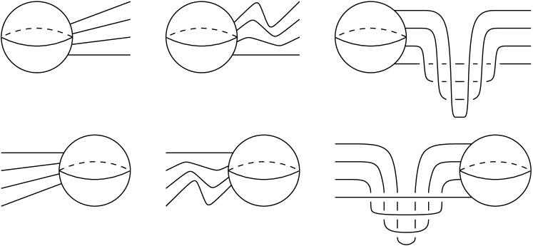
Figure 18. Perturbing the $xz$ projection of a Legendrian link near the attaching locus (left) to obtain the $xz$ projection of a link (middle) whose $xy$ projection (right) contains a dip. This produces new Reeb chords near the attaching locus.

Lemma 5.11.

There exists an isotopy such that for any Reeb chord $c\in{\mathcal{N}}$, the action ${\mathfrak{a}}(c)$ of $c$ satisfies ${\mathfrak{a}}(c)<2\delta_{1}$.

Proof.

Figure 19 shows the front of the link before and after the isotopy. The lemma follows. ∎

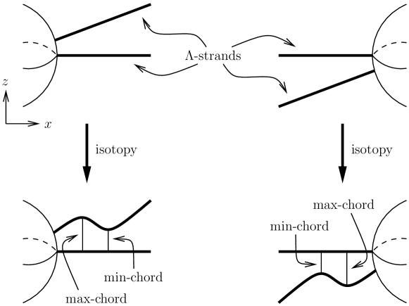
Figure 19. Short chords introduced by the isotopy. In each diagram, the height of the vertical direction is less than $\epsilon$.

We call a Legendrian link obtained by front resolution followed by an attaching isotopy introducing short chords a Legendrian link with split diagram. We show below that the holomorphic disks which need to be considered for calculation of the differential of the Legendrian homology a Legendrian link with split diagram are of three types: diagram disks, handle disks, and interpolating disks.

5.3.B. Diagram disks

Let $\Lambda$ be a Legendrian link with split diagram. Let $R(r_{1})\subset R(r_{2})\subset\mathbb{R}^{2}$, where we think of $\mathbb{R}^{2}$ as the $xy$-plane, be regions such that $R(r_{2})$ contains all of the diagram of $\Lambda$ except standard strands entering the attaching locus and such that $R(r_{2})-R(r_{1})$ contains all the diagram double points corresponding to the short maximum Reeb chords near the attaching locus, see Figure 19.

Lemma 5.12.

Let $u\colon D\to\mathbb{R}\times Y_{k}(\delta)$ be a holomorphic disk with one positive puncture and boundary on $\mathbb{R}\times\Lambda$. Assume that the Reeb chord of the positive puncture is contained in $R(r_{1})\times\mathbb{R}\subset Y_{k}(\delta)$. Then $u(D)$ is contained in $\mathbb{R}\times(R(r_{1})\times\mathbb{R})$.

Proof.

Recall that we use the $\mathbb{R}$-invariant almost complex structure pulled back from ${\mathbb{C}}$ in $\mathbb{R}\times(R(r_{1})\times\mathbb{R})$. Let $E=u^{-1}(\mathbb{R}\times(R(r_{2})\times\mathbb{R}))$. Then for generic $r_{2}$, $E$ is a Riemann surface with boundary $\partial E$ mapping to

$$(\mathbb{R}\times\Lambda)\,\,\cup\,\,(\mathbb{R}\times(\partial R(r_{2})\times\mathbb{R})),$$

and if $\pi\colon\mathbb{R}\times(R(r_{2})\times\mathbb{R})\to R(r_{2})$ is the projection then $\pi\circ u$ is holomorphic with respect to the standard complex structure on ${\mathbb{C}}$. If $u$ does not map any boundary component into $\mathbb{R}\times(R(r_{2})-R(r_{1}))\times\mathbb{R}$ then it is an easy consequence of the maximum principle that $u(D)\subset R(r_{1})$: if not $u|_{E}$ would not have bounded $y$-coordinate and its area would be infinite.

Assume thus that some boundary component of $D$ maps into this region. Consider the outermost strand before the dip. As above, the maximum principle implies that the disk cannot lie on the outside of this strand. Hence it lies on the inside. If the disk has no more corners then it eventually ends up on the outside and the maximum principle again is violated. It follows that the disk stays in $\mathbb{R}\times(R(r_{1})\times\mathbb{R})$. ∎

We call disks in Lemma 5.12 diagram disks.

5.3.C. Handle disks

Consider a standard Legendrian strand $\Lambda$ running through a one-handle, see Section 4.2.A. Recall that the Reeb chords of $\Lambda$ are then $c^{m}$, $m=1,2,\dots$ where $m$ is the number of times the chord wraps around the central Reeb orbit and that although all chords are orbits, they are nondegenerate in the sense that the linearized Reeb flow takes the tangent space of $\Lambda$ at the start point to a Lagrangian subspace in the contact plane in the tangent space at the endpoint which is transverse to the tangent space of $\Lambda$ at the end point. Consider a small perturbation of the standard strand so that no Reeb chord is also an orbit. Then the Reeb chords are in natural one-to-one correspondence with the Reeb chords of the unperturbed strand and we then have the following.

Lemma 5.13.

The moduli space ${\mathcal{M}}^{\mathbb{R}\times Y_{k}(\delta)}(c^{1};\varnothing)$ of once punctured holomorphic disks with boundary on $\Lambda\times\mathbb{R}$ contains algebraically one $\mathbb{R}$-family (i.e., one disk, rigid up to translation).

Proof.

Consider the Weinstein domain obtained by attaching one $1$-handle to the ball. Let $\Lambda$ denote the standard Legendrian knot which runs through the handle once. Then the Weinstein manifold which results from attaching a $2$-handle along $\Lambda$ is the $4$-ball. According to [5, Corollary 5.7] there is a quasi-isomorphism between the symplectic homology of the ball and the homology of a complex $A^{\rm Ho}(\Lambda)$ associated to $A(\Lambda)$ that has two generators for each monomial $w$ in $A(\Lambda)$, $\hat{w}$ and $\check{w}$:

$$SH(B^{4})\to A^{\rm Ho}(\Lambda).$$

Now the complex on the left hand side is acyclic and the complex of the right hand side has no generators in negative degrees, one generator $\tau$ in degree $0$, and one generator $\check{c}^{1}$ in degree $1$. Since the homology must vanish we conclude that

$$d_{A^{\rm Ho}}\check{c}^{1}=\tau.$$

On the other hand $\langle d_{A^{\rm Ho}}\check{c}^{1},\tau\rangle$ can be computed in terms of moduli spaces of holomorphic disks:

$$\langle d_{A^{\rm Ho}}\check{c}^{1},\tau\rangle=|{\mathcal{M}}^{Y_{k}(\delta)}(c^{1};\varnothing)|,$$

where the right hand side denotes the number of $\mathbb{R}$-components in the moduli space. The lemma follows. ∎

Remark 5.14.

Alternatively, one can prove Lemma 5.13 using Remark 2.23 as follows. Since the closed up standard strand is isotopic to a stabilization it is straightforward to show that its DGA must be trivial. This implies that $1$ is a boundary which gives the desired result as explained above.

We next construct a somewhat nongeneric situation where many strands pass through the handle but where all the relevant moduli spaces admit concrete descriptions. Fix a $1$-jet neighborhood of $\Lambda_{\rm st}$ and fix a very small $\epsilon>0$. Consider $n$ strands $\Lambda_{1}^{\prime},\dots,\Lambda_{n}^{\prime}$ parallel to $\Lambda_{\rm st}$. More precisely, let

$$\Lambda_{j}^{\prime}=\Phi^{j\epsilon}_{R}(\Lambda_{\rm st}),$$

where $\Phi_{R}^{t}$ is the time $t$ Reeb flow. Then $\Lambda_{j}^{\prime}$ is Legendrian for $j=1,\dots,n$.

Lemma 5.15.

The Reeb chords connecting $\Lambda_{j}^{\prime}$ to $\Lambda_{k}^{\prime}$ are as follows:

• If $j<k$ then: there is one Reeb chord of length $(k-j)\epsilon$ starting at any point on $\Lambda_{j}^{\prime}$, for each integer $w>0$ there is a Reeb chord along the unique Reeb orbit in the handle of length $2\pi w\delta+(k-j)\epsilon$, and there are no other Reeb chords.

• If $j\geq k$ then: for each integer $w>0$ there is a Reeb chord along the unique Reeb orbit in the handle of length $2\pi w\delta-(j-k)\epsilon$, and there are no other Reeb chords.

Proof.

Consider ${\rm(a)}$. Note that any Reeb chord starting on $\Lambda_{j}^{\prime}$ and ending on $\Lambda_{k}^{\prime}$ gives rise to a Reeb chord starting and ending on $\Lambda_{k}^{\prime}$ by subtracting one of the short Reeb chords mentioned. Similarly, in case ${\rm(b)}$, any Reeb chord stating on $\Lambda_{j}$ and ending on $\Lambda_{k}^{\prime}$ gives rise to a Reeb chord starting and ending on $\Lambda_{j}^{\prime}$ by adding one of the short chords.

Since $\Lambda_{j}^{\prime}=\Phi^{j\epsilon}_{R}(\Lambda_{\rm st})$ the lemma follows from Lemma 4.3. ∎

In order to get to a situation where the moduli spaces can be described we perturb $\Lambda_{j}^{\prime}$ further as follows. In the $1$-jet neighborhood $\Lambda_{j}^{\prime}$ corresponds to the graph of the constant function $f(q)=j\epsilon$. We denote the perturbation of $\Lambda_{j}^{\prime}$ by $\Lambda_{j}$ and define it as the $1$-jet graph of the function $f(q)=j\epsilon+j\kappa q^{2}$, where $\kappa\ll\epsilon$ and where $q$ is a coordinate along the standard strand. (Note that $q=0$ corresponds to the central Reeb orbit.)

Lemma 5.16.

The Reeb chords connecting $\Lambda_{j}$ to $\Lambda_{k}$ are as follows:

• If $j<k$ then for each integer $w\geq 0$ there is a Reeb chord along the unique Reeb orbit in the handle of length $2\pi w\delta+(k-j)\epsilon$, and there are no other Reeb chords.

• If $j\geq k$ then for each integer $w>0$ there is a Reeb chord along the unique Reeb orbit in the handle of length $2\pi w\delta-(j-k)\epsilon$, and there are no other Reeb chords.

Proof.

To control short Reeb chords one may use the $1$-jet neighborhood. Uniqueness of short chords is then an immediate consequence of the fact that functions of the form $f(q)=c_{0}+c_{2}q^{2}$, $c_{0},c_{2}$ constants, have only one critical point at the origin. For the long chords simply note that no strand was perturbed at its intersection with the central Reeb orbit and that for all long chords, the linearized Reeb flow mapped the tangent line at the initial point to a tangent line transverse to the tangent line in the contact plane at the final point already for $\Lambda_{0}^{\prime},\dots,\Lambda_{n}^{\prime}$. ∎

We will use the following notation for Reeb chords between the strands $\Lambda_{1},\dots,\Lambda_{n}$: let $c_{ij}^{p}$ be the Reeb chord connecting $\Lambda_{j}$ to $\Lambda_{i}$ of length closest to $2\pi\delta p$. Using the definition of Reeb chord grading from [5, Section 2.1], it is a straightforward consequence of Lemma 4.2 that the grading of $c^{p}_{ij}$ is

$$|c^{p}_{ij}|=2p-1+m(i)-m(j),$$

where $m(i)$ denotes the integer valued Maslov potential of the strand $\Lambda_{i}$, see Section 2.3.

Lemma 5.17.

For sufficiently small perturbations $\Lambda_{1},\dots,\Lambda_{n}$ of $\Lambda_{\rm st}$ as described above the following holds. If $i,j,l\in\{1,\dots,n\}$ and if $m,p,q\geq 0$ with $m=p+q$, then the moduli space ${\mathcal{M}}(c^{m}_{ij};c^{p}_{lj},c^{q}_{il})$ is transversely cut out and $C^{1}$-diffeomorphic to $\mathbb{R}$. Furthermore, moduli spaces of holomorphic disks with all punctures inside the handle and with more than two negative punctures have formal dimension $>1$.

Proof.

To see the last statement note that if the positive puncture maps to $c^{p}_{ij}$ and the negative punctures map to chords $c^{q_{l}}_{ij}$ then $p\geq\sum q_{l}$ for action reasons and the grading formula shows that the dimension of the moduli space is $>1$ if there are more than two negative punctures.

Now consider the $1$-parameter family (including $\mathbb{R}$-translation) of disks shown in Figure 20. We claim first that it is transversely cut out. To this end we use the trivialization $x_{2}+iy_{2}$ for the normal bundle of the disk. We trivialize the bundle over the Reeb chords which leads to a Lagrangian boundary condition given by small rotations which when closed up by negative rotations at corners has Maslov index equal to $-1$. The operator is Fredholm of index $0$ with values in a $1$-dimensional bundle. It follows that it is an isomorphism.

We next show that this is the only disk (up to $\mathbb{R}$-translation) in the moduli space. To see this we note that if there were another disk in the moduli space then it could not be contained in the Reeb orbit cylinder over $c^{m}$. This however contradicts its action being $0$ and we conclude there is exactly one disk. ∎

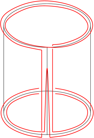
Figure 20. A rigid disk in a handle covering a Reeb orbit cylinder.

By Lemma 5.6, disks that contribute to the differential and that start inside the handle cannot have negative punctures outside the handle.

5.3.D. Interpolating curves

Finally, we consider curves that start outside the handle and go inside. An action argument shows that they cannot leave a small neighborhood of the standard strand. It follows that they lie entirely in the $1$-jet neighborhood and hence are given by a count of holomorphic polygons on the diagram in the cotangent bundle in a neighborhood of the $0$-section, just like in the $\mathbb{R}^{3}$-case identifying the $0$-section with the $x$-axis and the cotangent fibers with lines in $y$-direction.

5.4. Orientations and signs

In this section we present an orientation scheme and compute the corresponding signs of the rigid disks described in Section 5.3. The material presented here is a generalization of [12, Section 4.5] and we will refer there for many details.

5.4.A. A trivialization of the bundle of contact planes in $Y_{k}(\delta)$

Consider first the standard contact $\mathbb{R}^{3}$ with contact form $\alpha_{\rm st}=dz-y\,dx$. As above we use the complex structure on the contact planes induced by the standard complex structure on $T^{\ast}\mathbb{R}={\mathbb{C}}$ via the Lagrangian projection $\Pi\colon\mathbb{R}^{3}=J^{1}(\mathbb{R})\to T^{\ast}\mathbb{R}$. Furthermore we trivialize the contact plane field using the frame $\partial_{y},J\partial_{y}$ where $J$ is the complex structure on the contact plane field. We next transport this trivializing vector field to the standard contact balls. Recall the contactomorphism in (4.8). Its inverse is

$$F^{-1}(x,y,z)=(x-x_{0}\,,\,y-y_{0}\,,\,z-z_{0}-\tfrac{1}{2}(x-x_{0})(y+y_{0})).$$

In particular, the vector field corresponding to $\partial_{y}$ is then

(5.2) $$dF^{-1}\,\partial_{y}=\partial_{v}-\tfrac{1}{2}u\,\partial_{z}.$$

We next study the behavior of trivializations in the handles of $Y_{k}(\delta)$. Recall the trivialization of the contact plane field along $V_{-\delta}$ given by $v,i\cdot v$, where $i$ is the complex structure of ${\mathbb{C}}^{2}$ and where $v$ is given by (4.2). In our construction of $Y_{k}(\delta)$ we attached the handles using standard contact balls identified with balls in $V_{-\delta}$. The identifications were constructed using the map of the disks in (4.9) and (4.10). In order to determine the vector field in the standard ball that corresponds to $v$, we first express $v$ as

$$v=w_{0}+w_{R},$$

where $w\in TA_{\rho}$ and where $w_{R}$ is parallel to the Reeb vector field. Using notation as in (4.3), we find

$$w_{0}=y_{2}\partial_{y_{1}}+\tfrac{1}{2}y_{1}\partial_{y_{2}},\qquad w_{R}=-\tfrac{1}{2}x_{1}y_{2}^{-1}\,\tilde{R}.$$

The vector field $v_{\rm b}$ in the standard contact ball that corresponds to $v$ is thus the sum of the image of $w_{0}$ under $dG$, see (4.10), and a suitable multiple of the Reeb field. A straightforward computation gives

$$v_{\rm b}=-\tfrac{1}{2}u\left(\delta^{2}+\tfrac{1}{4}(u^{2}+v^{2})\right)\partial_{z}+\left(\delta^{2}+\tfrac{3}{4}u^{2}+\tfrac{1}{2}v^{2}\right)\partial_{v}+\tfrac{1}{2}uv\,\partial_{u}.$$

Continuously killing all quadratic terms, we find a homotopy to the trivialization given by

$$-\tfrac{1}{2}u\,\partial_{z}+\partial_{v},$$

which in turn corresponds to the vector field $\partial_{y}$ in $1$-jet coordinates. In conclusion, we have continued the trivialization of the contact plane field given by $(\partial_{y},J\partial_{y})$ over $\mathbb{R}^{3}(\circ_{k})$ to all of $Y_{k}(\delta)$ in such a way that inside the handles this trivialization is given by $(v,i\cdot v)$.

5.4.B. Capping operators and the symplectization direction

In [12] the contact manifolds under consideration are of the form $P\times\mathbb{R}$, where $P$ is an exact symplectic manifold, with contact form $dz-\beta$, where $\beta$ is the primitive of the symplectic form on $P$. (In particular, taking $P=T^{\ast}\mathbb{R}$ and $\beta=y\,dx$, we get standard contact $\mathbb{R}^{3}$ as a special case.) If we use an almost complex structure on the symplectization of such a manifold given by the product of the standard complex structure on ${\mathbb{C}}\approx\mathbb{R}\times\mathbb{R}$ and the pullback to the contact planes of an almost complex structure on $P$, holomorphic curves in the symplectization can be described entirely in terms of holomorphic curves in $P$, and it was moduli spaces of holomorphic curves in $P$ that were oriented in [12]. In the present setup we do not have any projection and hence we must study holomorphic curves in the symplectization. As a starting point we will revisit the construction in [12], in a sense adding the symplectization direction back.

5.4.C. A brief description of the orientation scheme

We give the description as close as possible to the application we have in mind. The starting point is a number of properties of $\bar{\partial}$-operators with Lagrangian boundary conditions on the disk that we discuss next. These properties originate from [18]; we will however refer to [12] since the treatment there is closer to the case under study here. Let $D$ denote the unit disk in ${\mathbb{C}}$ and let $L\colon\partial D\to\operatorname{Lag}({\mathbb{C}}^{2})$ denote a smooth map where $\operatorname{Lag}({\mathbb{C}}^{2})$ denotes the space of Lagrangian planes in ${\mathbb{C}}^{2}$. Consider the Riemann–Hilbert problem with trivialized Lagrangian boundary condition: let $W_{2}(L)$ denote the space of functions $u\colon D\to{\mathbb{C}}^{2}$ with two derivatives in $L^{2}$ such that

$$u(e^{i\theta})\in L(e^{i\theta}),\quad\quad L\bar{\partial}_{J}u|_{\partial D}=0,$$

and let $W_{1}$ denote the space of $J$-complex-antilinear maps $TD\to T{\mathbb{C}}^{2}$ with one derivative in $L^{2}$ that vanish when restricted to the boundary, or equivalently, after fixing a trivialization of $TD$, the corresponding space of maps $D\to{\mathbb{C}}^{2}$. Then the linearized operator $L\bar{\partial}_{J}\colon W_{2}(L)\to W_{1}$ is a Fredholm operator of index

$$2+\mu(L),$$

where $\mu(L)$ denotes the Maslov index of $\Lambda$. If $Y^{\prime}$ denotes the space of Fredholm operators as just described, then the determinant bundle over $Y^{\prime}$ with fiber over $L\in Y$ given by

$$\Lambda^{\rm max}\left(\operatorname{ker}(L\bar{\partial}_{J})\right)\otimes\Lambda^{\rm max}\left(\operatorname{coker}(L\bar{\partial}_{J})\right)$$

is nonorientable and remains nonorientable if $Y^{\prime}$ is replaced by the space of oriented Lagrangian boundary conditions. However, adding the requirement that the bundle of Lagrangian subspaces over $\partial D$ is trivialized leads to an orientable bundle, see [12, Lemma 3.8]. Note that the space of trivialized Lagrangian boundary conditions is homotopy equivalent to $\Omega(U(2))$, the loop space of the unitary group of ${\mathbb{C}}^{2}$: if $A\colon\partial D\to U(2)$ then $A\cdot\mathbb{R}^{2}$ is a trivialized Lagrangian boundary condition and an orthonormal frame in a Lagrangian plane gives an element in $U(2)$. Furthermore, as explained in [12, Lemma 3.8], orientations on $\mathbb{R}^{2}\subset{\mathbb{C}}^{2}$ and on ${\mathbb{C}}$ induce an orientation on the determinant bundle over $Y$. We use this orientation of the determinant bundle over $Y$ to orient all moduli spaces.

Let $\Lambda\subset Y_{k}(\delta)$ be a Legendrian link and consider a moduli space${\mathcal{M}}^{\mathbb{R}\times Y_{k}(\delta)}(a;b_{1},\dots,b_{k})$. In order to orient it we first fix a trivialization $\tau$ of the tangent bundle of $\Lambda$. Then $(\partial_{t},\tau)$ gives a trivialization of the tangent bundle of $\mathbb{R}\times\Lambda\subset\mathbb{R}\times Y_{k}(\delta)$, where $\partial_{t}$ is the vector field along the $\mathbb{R}$-factor of $\mathbb{R}\times Y_{k}(\delta)$. Note that if $u\colon D_{k+1}\to\mathbb{R}\times Y_{k}(\delta)$ is a holomorphic map of a $(k+1)$-punctured disk with boundary on $\mathbb{R}\times\Lambda$, then $u^{\ast}T(\mathbb{R}\times Y_{k}(\delta))$ splits as $u^{\ast}(\operatorname{ker}(\alpha))\oplus{\mathbb{C}}$, and the Lagrangian boundary condition splits as $u^{\ast}(T\Lambda)\oplus\mathbb{R}$. Second we fix positive and negative oriented capping operators at all Reeb chords. These are $1$-punctured disks with trivialized Lagrangian boundary conditions, which when glued to the punctures give a disk with trivialized boundary condition.

In [12, Section 3.2], (linear) gluing analysis for joining operators as just described is carried out. In particular, if $k+2$ operators are glued into an operator then orientations on the determinants of all operators except one induce an orientation on the last one. (The actual rule for how to induce such an orientation depends on some choices that are discussed in detail in [12].) In particular, capping operators allow us to orient the kernel/cokernel of the linearized operator at $u$, which together with a chosen fixed orientation on the space of automorphisms/conformal structure on $D_{k+1}$ gives an orientation of the moduli space.

5.4.D. Signs of diagram disks

The main objective of this section is to reduce the computation of the sign of a diagram disk to the computation of similar disks carried out in [12, Section 4.5]. Consider the four quadrants at a crossing of the link diagram as in the right diagram in Figure 5. In the terminology of [12], quadrants where the sign is $-1$ are called $A$-shaded. We then have the following:

Lemma 5.18.

Let $T\Lambda$ be equipped with the Lie group spin structure. Then there is a choice of orientation of ${\mathbb{C}}$ and $\mathbb{R}$ such that the sign of a rigid diagram disk in ${\mathcal{M}}(a;b_{1},\dots,b_{k})$ is given by $(-1)^{s(u)}$ where $s(u)$ is the number of $A$-shaded corners of $u$.

We prove Lemma 5.18 after discussing capping operators. Here we use the observation above that the boundary condition of the linearized operator splits and define split capping operators. For the component of the boundary condition at a Reeb chord in the contact plane we use exactly the same capping operators as in [12, Section 4.5]. (As there, this requires stabilization in order to have room to rotate the trivialization so that it satisfies compatibility conditions at Reeb chord endpoints.) In the symplectization direction, the tangent space to the configuration space of maps around a solution is a Sobolev space with small positive weight near each puncture, augmented by a $1$-dimensional space of explicit solutions near each puncture corresponding to translations in the $\mathbb{R}$-direction. The kernel and cokernel of the corresponding linearized problem are canonically identified with the kernel and cokernel of the same (linearized) operator acting on the Sobolev space with small negative exponential weight and without auxiliary space of solutions. We thus use as capping operators in the symplectization directions the once-punctured disk with constant boundary condition $\mathbb{R}$ and with small negative exponential weight. This operator has index $1$ and has $1$-dimensional kernel. The gluing sequence for the capping disks with positive (respectively, negative) punctures, which glue to the constant boundary condition on the closed disk, again of index $1$ with $1$-dimensional kernel, is:

$$\begin{CD}0@>{}>{}>\ker(\bar{\partial}_{D})@>{}>{}>\ker(\bar{\partial}_{D_{+}})\oplus\ker(\bar{\partial}_{D_{-}})@>{}>{}>\mathbb{R}@>{}>{}>0.\end{CD}$$

Here $\bar{\partial}_{D_{+}}$ and $\bar{\partial}_{D_{-}}$ denote the capping operators in the $\mathbb{R}$-direction with positive (respectively, negative) puncture, $\bar{\partial}_{D}$ denotes the operator on the closed disk with constant $\mathbb{R}$ boundary condition, and the last $\mathbb{R}$ is identified with the cokernel of the $\bar{\partial}$-operator on the strip with $\mathbb{R}$-boundary conditions and positive exponential weights at both ends. (This cokernel consists of constant functions with values in $i\mathbb{R}$ and the operator is the operator on the middle part of the glued disk as the gluing parameter goes to $\infty$.) The maps in the sequence are given by the matrices

$$\left(\begin{matrix}1\\ 1\end{matrix}\right)\quad\text{ and }\quad\left(\begin{matrix}-1&1\end{matrix}\right).$$

Consider next the gluing sequence for the ${\mathbb{C}}$-component of a linearized boundary condition. Note that the result of gluing capping operators to the linearized boundary condition is again a closed disk with constant boundary condition $\mathbb{R}$ and $1$-dimensional kernel, and the gluing sequence is

$$\begin{CD}0@>{}>{}>\ker(\bar{\partial}_{D})@>{}>{}>\ker(\bar{\partial}_{D_{+}})\oplus_{j=1}^{m}\ker(\bar{\partial}_{D_{-};j})\oplus\ker(\bar{\partial}_{{\mathbb{C}}})@>{}>{}>\\ {}@>{}>{}>\oplus_{j=1}^{m}\mathbb{R}@>{}>{}>0,\end{CD}$$

where the summands are gluing parameters near the punctures. Thus the orientation induced on $\ker(\bar{\partial}_{{\mathbb{C}}})$ is simply the orientation induced by the $\mathbb{R}$-factor.

Proof of Lemma 5.18.

By our choice of capping operators and the linear gluing that this gives rise to, as discussed above, it follows that the orientation of the reduced moduli space is determined entirely in terms of the operator in the contact planes which is pulled back from ${\mathbb{C}}$ for diagram disks. The lemma is then an immediate corollary of [12, Theorem 4.32]. ∎

5.4.E. Signs of interpolating disks

After the signs of diagram disks have been computed, the sign of interpolating disks can be determined by a simple homotopy argument. More precisely, we have the following:

Lemma 5.19.

Let $T\Lambda$ be equipped with the Lie group spin structure. Then there is a choice of orientation of ${\mathbb{C}}$ and $\mathbb{R}$ such that the sign of a rigid interpolating disk in ${\mathcal{M}}(a;b_{1},\dots,b_{k})$ is given by $(-1)^{s(u)}$ where $s(u)$ is the number of $A$-shaded corners of $u$. Here the diagram disk should be drawn in a $1$-jet neighborhood of $\Lambda_{\rm st}$.

Proof.

By monotonicity any rigid holomorphic connecting disk lies in an arbitrarily small neighborhood of $\Lambda_{\rm st}$ and its Lagrangian projection has convex corners. Furthermore, it can be homotoped through disks with convex corner to a small such disk in $\mathbb{R}^{2}$. The result then follows from Lemma 5.18 once we choose capping operators as there for the short Reeb chords in the handle. ∎

5.4.F. Signs of handle disks

We now turn to determining the signs of rigid handle disks. In order to determine the signs of interpolating disks, we made choices for the orientations of the capping disks with positive puncture at the short Reeb chords in the middle of the handle. We choose here also the capping disks with negative puncture as for the diagram disks, and the orientation on the determinants of the corresponding operators are then fixed by the condition that these two orientations should glue to the canonical orientation. Note next that the linearized boundary condition of a rigid handle disk with positive puncture at a short Reeb chord in the middle of the handle can be deformed to that of a small rigid triangle lying in the $1$-jet neighborhood of $\Lambda_{\rm st}$. It follows from Lemma 5.19 that the sign of any such rigid disk in ${\mathcal{M}}(c^{0}_{ij};c^{0}_{il},c^{0}_{lj})$ is

$$(-1)^{|c^{0}_{il}|+1}.$$

Before we complete the discussion of combinatorial signs we need to recall an orientation gluing result: with capping operators fixed and oriented in such a way that orientations on positive and corresponding negative caps glue to the canonical orientation on the determinant of the operator on the closed disk, the following holds. If $I\subset\hat{\mathcal{M}}(a;b_{1},\dots,b_{m})$ is a component of a reduced moduli space of dimension $1$ with nonempty boundary which is oriented as above, and if $u_{0}\#v_{0}$ and $u_{1}\#v_{1}$ are the broken disks at its two boundary points, then

(5.3) $$\sigma(u_{1})\epsilon(u_{1},v_{1})\sigma(v_{1})+\sigma(u_{0})\epsilon(u_{0},v_{0})\sigma(v_{0})=0,$$

where $\sigma(u)$ is the sign of the rigid disk $u$ and where

$$\epsilon(u,v)=(-1)^{\sum_{j=1}^{l}|b_{j}|},$$

if $u\in{\mathcal{M}}(a;b_{1},\dots,b_{l},b_{l+1},\dots,b_{m})$ and $v\in{\mathcal{M}}(b_{l+1};c_{1},\dots,c_{k})$. This follows from [12, Lemma 4.11] in combination with the above discussion of capping operators in the symplectization direction. Using this property we can establish a combinatorial sign rule inductively.

Lemma 5.20.

There is a choice of orientations for capping operators at the Reeb chords inside the handle for which the sign of the rigid disk in ${\mathcal{M}}(c^{p}_{ij};c^{q}_{il},c^{r}_{lj})$ equals

$$(-1)^{|c^{q}_{il}|+1}.$$

Proof.

After the above discussion of short chords, we may assume that the sign rule holds for all rigid triangles with positive puncture below a given action. Consider the next Reeb chord $a$ in the action ordering. We claim that if we choose the orientation on the capping operator of $a$ as a positive puncture so that the sign rule holds for some triangle with positive puncture at $a$, then it holds for all such triangles. To see this, we represent the link as $\Lambda_{1}\cup\dots\cup\Lambda_{n}$ inside the handle exactly as in Lemma 5.17. Then any rigid triangle lies inside the trivial holomorphic cylinder over the central Reeb chord and looks like a Reeb chord strip with a slit, see Figure 20. For any two such triangles we get a transversely cut out reduced $1$-dimensional moduli space by considering the corresponding strip with two slits. Assume that this moduli space is ${\mathcal{M}}(a;b_{1},b_{2},b_{3})$. Then its boundary points correspond to

$$(u_{0},v_{0}) \in{\mathcal{M}}(a;b_{1},b_{23})\times{\mathcal{M}}(b_{23};b_{2},b_{3}),$$

$$(u_{1},v_{1}) \in{\mathcal{M}}(a;b_{12},b_{3})\times{\mathcal{M}}(b_{12};b_{1},b_{2}),$$

and our inductive assumption implies that

$$\sigma(v_{0})=(-1)^{|b_{2}|+1}\quad\text{ and }\quad\sigma(v_{1})=(-1)^{|b_{1}|+1}.$$

Equation (5.3) then gives

$$(-1)^{|b_{1}|+1}\left(\sigma(u_{0})(-1)^{|b_{2}|}+\sigma(u_{1})\right)=0.$$

Since $|b_{12}|=|b_{1}|+|b_{2}|+1$, it follows that $\sigma(u_{0})=(-1)^{|b_{1}|+1}$ if and only if $\sigma(u_{1})=(-1)^{|b_{12}|+1}$. By induction, we conclude that the lemma holds. ∎

Appendix A Invariance from an analytical perspective

In this section we adapt the standard SFT proof of invariance to show that the homotopy type of the DGA $A(\Lambda)$ for a Legendrian link $\Lambda\subset Y_{k}(\delta)$ depends only on the isotopy class of $\Lambda$. As mentioned in the Introduction, this is a proof strategy rather than a proof since it depends on a perturbation scheme for M-polyfolds that has not yet been fully worked out.

Consider an isotopy $\Lambda_{t}$, $t\in[0,1]$, between Legendrian links $\Lambda_{0}$ and $\Lambda_{1}$. The isotopy then gives an exact Lagrangian $L_{01}\subset Y_{k}(\delta)$ with positive end $\Lambda_{0}$ and negative end $\Lambda_{1}$. As mentioned in Section 5.1, this cobordism induces a DGA-morphism $\Phi_{01}\colon A(\Lambda_{0})\to A(\Lambda_{1})$. On the other hand, reversing the isotopy we get a corresponding map $\Phi_{10}\colon A(\Lambda_{1})\to A(\Lambda_{0})$ and by shortening the composite isotopy we get a $1$-parameter family of cobordisms $L_{00}^{s}$, $s\in[0,1]$, with induced map at $s=0$ given by $\Phi_{10}\circ\Phi_{01}$ and at $s=1$ given by the identity. Thus, once we prove that a $1$-parameter family of cobordisms induces a chain homotopy, we can conclude that $\Phi_{10}\circ\Phi_{01}$ is chain homotopic to the identity. Similarly, $\Phi_{01}\circ\Phi_{10}$ is chain homotopic to identity and invariance will follow.

Below we will discuss some of the steps in this program, following [11].

A.1. Anchored disks

Consider a generic $1$-parameter family of cobordisms $L_{s}\subset Y(\delta)\times\mathbb{R}$, $s\in[0,1]$. In order to define the chain homotopy $K$ induced by $L_{s}$ we will consider the boundary of $1$-dimensional parameterized moduli spaces. That in turn involves looking at holomorphic disks of formal dimension $-1$. Using the argument from [13, Lemma 4.5(1)] as in Section 5.1, it is straightforward to show that disks with one positive boundary puncture and several negative boundary and interior punctures are transversely cut out after a small perturbation of the almost complex structure $J$. Recall that the Conley–Zehnder indices of the Reeb orbits in $Y_{k}(\delta)$ are $2m$, $m>0$. Thus, possible dimensions of spaces of holomorphic disks are $2m-1$. Let $\gamma$ be a simple central Reeb orbit in the middle of a handle, and let ${\mathcal{M}}^{X}(\gamma)$ denote the moduli space of holomorphic disks with positive puncture at $\gamma$.

Lemma A.1.

For generic $J$, the space ${\mathcal{M}}^{X}(\gamma)$ is a transversely cut out $1$-manifold with boundary points corresponding to $\mathbb{R}$-families in the moduli space ${\mathcal{M}}^{\mathbb{R}\times Y_{k}(\delta)}(\gamma)$.

Proof.

Since the Reeb orbit is simple the moduli space cannot contain multiple covers. Hence any curve in it is somewhere injective and the transversality follows from a standard argument. Since the Reeb orbit has minimal action there can be no bubbling and the boundary is as claimed. ∎

Remark A.2.

It follows from the Bott–Morse description of symplectic homology that the moduli spaces ${\mathcal{M}}^{X}(\gamma)$ in fact are nonempty, since curves in them constrained by the unstable manifold of the critical point in the handle are needed for the symplectic homology differential to hit the corresponding Morse generator, which must be hit since the symplectic homology of a subcritical Weinstein manifold vanishes [8].

A.2. Producing chain homotopies

Consider a $1$-parameter family of exact Lagrangian cobordisms $(Y_{k}(\delta),L_{s})$, $s\in[0,1]$, together with a $1$-parameter family of almost complex structures $J_{s}$. We assume that $J_{s}$ is such that parameterized moduli spaces of disks with one positive boundary puncture are transversely cut out, and that this holds also for the moduli spaces at the endpoints $s=0,1$. Write $\Lambda_{\pm}$ for the Legendrian submanifolds at the positive and negative ends of $L_{s}$. Then $L_{0}$ and $L_{1}$ determine chain maps

$$\Phi_{0},\Phi_{1}\colon A(\Lambda_{+})\to A(\Lambda_{-}).$$

Lemma A.3.

The DGA maps $\Phi_{0}$ and $\Phi_{1}$ are chain homotopic, i.e., there exists a finite sequence of chain maps $\Phi^{j}\colon A(\Lambda_{+})\to A(\Lambda_{-})$, $j=1,\dots,m$, with $\Phi^{1}=\Phi_{0}$ and $\Phi^{m}=\Phi_{1}$, and degree $+1$ maps $K^{j}\colon A(\Lambda_{+})\to A(\Lambda_{-})$, $j=1,\dots,m-1$, such that

(A.1) $$\Phi^{j+1}-\Phi^{j}=\Omega_{K^{j}}\circ\partial_{+}+\partial_{-}\circ\Omega_{K^{j}},$$

where $\partial_{\pm}$ is the differential on $A(\Lambda_{\pm})$ and where $\Omega_{K^{j}}$ is linear and is defined as follows on monomials:

$$\Omega_{K^{j}}(c_{1}\dots c_{r})=\sum_{l=1}^{r}(-1)^{|c_{1}|+\cdots+|c_{l-1}|}\Phi^{j+1}(c_{1}\cdots c_{l-1})K^{j}(c_{l})\Phi^{j}(c_{l+1}\cdots c_{r}).$$

Remark A.4.

The lemma follows from (a slightly extended version of) [11, Lemma B.15] (which involves orientations on the moduli spaces), which is stated in somewhat different terminology. In the proof below, we will adapt the terminology used there to the current setup. Also, it should be mentioned that [11, Lemma B.15] depends on a perturbation scheme for so-called M-polyfolds (the most basic level of polyfolds), the details of which were not yet worked out, and hence it should be viewed as a proof strategy rather than a proof in the strict sense.

Proof.

Write ${\mathcal{M}}^{s}(a;\mathbf{b})$ for the moduli space of (anchored) holomorphic disks in $Y_{k}(\delta)\times\mathbb{R}$ with boundary on $L_{s}$, positive puncture at the Reeb chord $a$, and negative punctures at the Reeb chords in the word $\mathbf{b}$. Consider a parameterized moduli space

$${\mathcal{M}}(a;\mathbf{b})=\bigsqcup_{s\in[0,1]}{\mathcal{M}}^{s}(a;\mathbf{b}),$$

where the $(L_{s},J_{s})$, $s\in[0,1]$, is generic.

We say that a holomorphic disk of formal dimension $d$ is a $(d)$-disk. Recalling that the Legendrian homology algebra is defined as a direct limit using the action filtration, we work below a fixed energy level. Since $(L_{s},J_{s})$ is generic, the $(-1)$-disks form a transversely cut-out $0$-manifold in the parameterized moduli space that is generic with respect to the projection to the parameter space. In particular this implies that $(-1)$-disks occur only at a finite number of isolated instances $0<s_{1}<s_{2}<\dots<s_{m}<1$ at which the cobordism contains exactly one $(-1)$-disk, and that the projection from the parameterized $1$-dimensional moduli space is a Morse function. It then follows that the chain maps $\Phi_{s}$ remain unchanged except possibly when $s$ crosses a $(-1)$-disk moment. We consider crossing such a $(-1)$-disk moment. For simpler notation we still take $s\in[0,1]$ and assume that there is a single $(-1)$-disk moment in the interval.

We first note that if the $(-1)$-disk has an interior puncture and gives an anchored $(0)$-disk, then it follows from Lemma A.1 that $\Phi_{s}$ does not change.

In order to express the change in the chain map at other $(-1)$-disk moments, we use the $(-1)$-disk to construct a chain homotopy. To do so one must however overcome a transversality problem that arises when several copies of the $(-1)$-disk are attached to a disk in the symplectization of the upper end, resulting in a non-transverse broken disk. To solve this problem we invoke so-called abstract perturbations. More precisely, a perturbation is constructed that orders the negative punctures of any disk in the upper end in time so that only one negative puncture can be attached to the $(-1)$-disk at the time. Note that since we start the perturbation from the degenerate situation where all negative punctures lie at the same time, new $(-1)$-disks might arise when the perturbation is turned on, where perturbations of a moduli space ${\mathcal{M}}^{\Lambda_{+}\times\mathbb{R}}(a;\mathbf{b})$ in the positive end might give new $(-1)$-disks with positive puncture at $a$.

The actual perturbation scheme is organized energy level by energy level in such a way that the the size of the time separation is determined by the action of the Reeb chord at the positive puncture. In particular the time distances between the positive punctures in the newly created $(-1)$-disk are of the size of this time separation. As we move to the next energy level, the time separation is a magnitude larger, so that one of the negative punctures of a disk on the new energy level passes all the positive punctures of the $(-1)$-disks created on lower energy levels before the puncture following it enters the region where $(-1)$-disks may be attached to it.

Consider now the parameterized $1$-dimensional moduli space ${\mathcal{M}}(a;\mathbf{b})$ of $(0)$-disks defined using the perturbation scheme just described. The boundary of ${\mathcal{M}}(a;\mathbf{b})$ then consists of the $0$-manifolds ${\mathcal{M}}^{0}(a,\mathbf{b})$ and ${\mathcal{M}}^{1}(a;\mathbf{b})$ as well as broken disks that consist of one $(-1)$-disk at $s$ and several $(0)$-disks with a $(1)$-disk in the upper or lower end attached. Thus, if for a Reeb chord $c$, $K(c)$ denotes the count of $(-1)$-disks after the ordering perturbation scheme is turned on:

$$K(c)=\sum_{|c|-|\mathbf{b}|=-1}\left|{\mathcal{M}}(c,\mathbf{b})\right|\mathbf{b},$$

then, by counting the boundary points of oriented $1$-manifolds, we conclude that (A.1) holds. ∎

Remark A.5.

The proof of invariance just given is in a sense less involved than the combinatorial proof given in Section B. In fact this comparison is a little misleading, the combinatorial proof should be compared to computing the chain homotopies associated to all relevant $(-1)$-moments rather than just proving existence, see [15]. For example, Gompf move 6 below involves an infinite sequence of birth-deaths of Reeb chords and the corresponding stable tame isomorphism involves a countably infinite stabilization, as does the chain map of the corresponding cobordism defined as a direct limit with respect to action.

Appendix B Invariance from a combinatorial perspective

In this section, we present proofs of various combinatorial results from Section 2 that have been deferred until now. We begin with the short proofs of Proposition 2.4 (about resolutions of fronts) and Proposition 2.8 ($\partial^{2}=0$) in Appendix B.1. The bulk of this section, Appendix B.2, consists of a proof of the main combinatorial invariance result, Theorem 2.18.

B.1. Proofs of Propositions 2.4 and 2.8

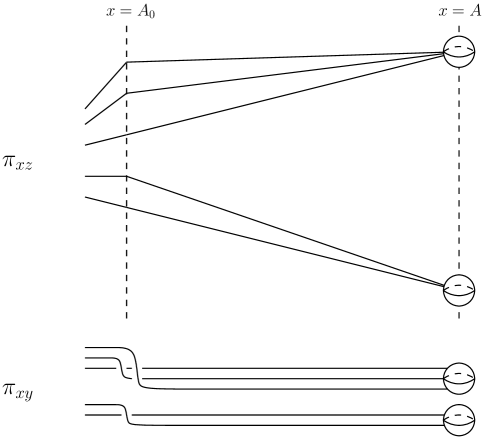
Figure 21. Setting up the rightmost portion of a front ($\pi_{xz}$) projection so that the corresponding $xy$ projection is the resolution of the front.

Proof of Proposition 2.4.

This follows the proof of Proposition 2.2 in [27]. Perturb a front in Gompf standard form to be the $xz$ projection of a tangle in normal form, as in Figure 2. Now beginning from the left, change the front by planar isotopy so that the corresponding $xy$ projection is given by the resolution of the front, as in [27]. The only novel feature in the current setup is that the right end of the front has to be arranged to pass into the $1$-handles (that is, strands passing into the same $1$-handle must become arbitrarily close in $z$ coordinate) while remaining in normal form.

Thus, suppose that we have constructed the front from left to right, including all crossings and cusps, and the only remaining task is to pass into the $1$-handles. Then the right-hand end of the front, where the front intersects say $x=A_{0}$ for some $A_{0}$, consists of a number of straight line segments whose slopes are increasing from bottom to top. Now for each $1$-handle, choose one strand of the Legendrian link that passes through that $1$-handle, and extend the corresponding straight line segment (with slope unchanged) rightward from $x=A_{0}$ to $x=A$ for some $A\gg A_{0}$. Then connect the $x=A_{0}$ endpoints of all strands passing through that $1$-handle to the endpoint of the chosen strand at $x=A$. See Figure 21 for an illustration.

For $A$ sufficiently large, the slopes of the line segments between $x=A_{0}$ to $x=A$ are, from bottom to top, increasing from handle to handle, and decreasing within the subset of strands passing into a single handle. Thus the corresponding $xy$ projection for $x\geq A_{0}$ looks precisely as desired: at $x=A_{0}$ there is a half twist involving the strands passing into each $1$-handle, and otherwise the $xy$ projection consists of horizontal lines. (To make the projection of the half twist generic, just perturb the $x=A_{0}$ endpoints slightly in the $x$ direction.) This completes the proof. ∎

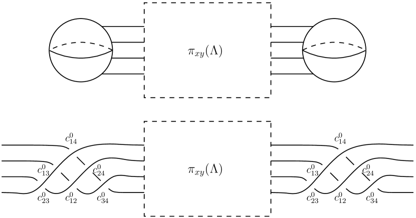
Figure 22. Turning a Legendrian link $\Lambda$ in $S^{1}\times S^{2}$ into a Legendrian tangle $\tilde{\Lambda}$ in $\mathbb{R}^{3}$.

Proof of Proposition 2.8.

The fact that this is true for generators of the internal DGA was noted in Section 2.3. Now suppose that $a_{i}$ is a crossing of $\pi_{xy}(\Lambda)$. We wish to show that $\partial^{2}(a_{i})=0$ and that $|\partial(a_{i})|=|a_{i}|-1$. We will assume for notational reasons that $\Lambda\subset S^{1}\times S^{2}$, but the same proof works for any number of $1$-handles.

Replace the $1$-handle in the $xy$ projection of $\Lambda$ by half-twists on the left and right, as in Figure 22. The result is the $xy$ projection of a Legendrian tangle $\tilde{\Lambda}$ in $\mathbb{R}^{3}$. To see this, add “dips” (cf. [30]) to $\Lambda$ on the left and right, and then the half-twists are half of each dip; see Figure 18 from Section 5.3.A. Let $n$ be the number of strands of $\Lambda$ passing through the $1$-handle. Label the crossings in the new half-twists in the tangle by $c_{ij}^{0}$, $1\leq i<j\leq n$, as shown in Figure 22 (note that these labels are repeated on left and right).

To the $xy$ projection of the Legendrian tangle $\tilde{\Lambda}$, we can associate a differential graded algebra over $\mathbb{Z}[\mathbf{t},\mathbf{t}^{-1}]$ just as in the standard Chekanov setup [7, 17], where the differential counts bounded disks (no unbounded regions) with boundary in $\pi_{xy}(\tilde{\Lambda})$. Here crossings are graded as usual by rotation numbers of paths from overcrossings to undercrossings, where the $2n$ ends of the tangle are identified pairwise; note in particular that this agrees with the grading of $c_{ij}^{0}$ from Section 2.4. For definiteness of orientation signs, at each of the crossings labeled $c_{ij}^{0}$, if $|c_{ij}^{0}|$ is even, then we take the south and west corners to be the $-1$ corners for orientation signs.

With these conventions, the Chekanov differential on the algebra for $\tilde{\Lambda}$ agrees with the differential $\partial$ on both the crossings $a_{i}$ in $\pi_{xy}(\Lambda)$ and on the $c_{ij}^{0}$. (In particular, this shows that $\partial(a_{i})$ is a finite sum of terms.) The usual proof that $\partial^{2}=0$ and $\partial$ lowers degree by $1$ from [7, 17] now gives the desired result. ∎

B.2. Combinatorial proof of invariance

B.2.A. Outline of the proof

In this section, we prove the main combinatorial invariance result, Theorem 2.18. The proof relies on establishing invariance under several elementary moves.

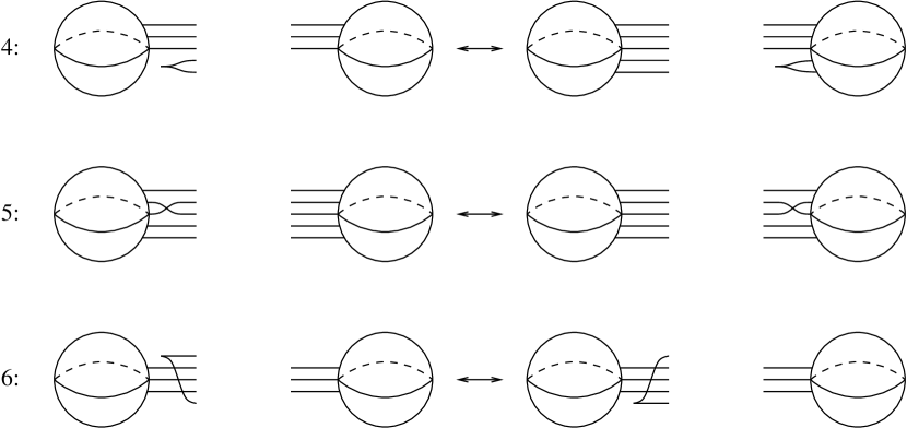
Figure 23. Gompf moves 4, 5, and 6.

More precisely, by Gompf [19], any Legendrian link in $\#^{k}(S^{1}\times S^{2})$ can be represented by a front diagram in Gompf standard form (see Section 2.1). Two such front diagrams represent links that are Legendrian isotopic if and only if they are related by a sequence of Legendrian isotopy of the front tangle inside the box $[0,A]\times[-M,M]$ (which can in turn be decomposed into a sequence of Legendrian Reidemeister moves as in $\mathbb{R}^{3}$), and three other moves, which we call Gompf moves 4, 5, and 6. See Figure 23. As mentioned in Section 2.2, we can perturb any diagram in Gompf standard form to a diagram in normal form, and the Gompf moves can be similarly perturbed to involve diagrams in normal form. We will henceforth assume that all front diagrams are in normal form.

We will prove invariance under each of Gompf’s moves; this is the content of Propositions B.3, B.5, B.9, and B.11 below. These results are then combined to prove Theorem 2.18 in Section B.2.H.

B.2.B. Reducing the number of possible moves

Before turning to the actual study of the DGA under moves, we consider two technical simplifications. First, Gompf’s version of move 4 in [19] has the cusped strands above the others, rather than below. The version we use, as shown in Figure 23, is equivalent to Gompf’s version, either by symmetry or by additional application of Gompf move 5.

Second, Gompf moves 4 and 6 have variants obtained from our diagrams by a $180^{\circ}$ rotation, which also need to be considered for a general Legendrian isotopy. However, we do not need to separately consider these alternate moves, because the action of $180^{\circ}$ rotation affects the DGA in a simple way, which we describe next.

Definition B.1 (cf. [24]).

Let $(\mathcal{A},\partial)$ be a semifree DGA over $R$ with generators $\{a_{i}\}$. There is another differential $\partial_{\textrm{op}}$ on $\mathcal{A}$ defined on generators by reversing the order of every word in $\partial(a_{i})$ and introducing appropriate signs. More precisely, define an $R$-module involution $\textrm{op}:\thinspace\mathcal{A}\to\mathcal{A}$ by

$$\textrm{op}(a_{i_{1}}a_{i_{2}}\cdots a_{i_{n}})=(-1)^{\sum_{j<k}|a_{i_{j}}||a_{i_{k}}|}a_{i_{n}}\cdots a_{i_{2}}a_{i_{1}},$$

and define $\partial_{\textrm{op}}=\textrm{op}\circ\partial\circ\textrm{op}$. Then $(\mathcal{A},\partial_{\textrm{op}})$ is another semifree DGA satisfying the Leibniz rule.

Lemma B.2.

Let $\Lambda$ be a Legendrian link in $\#^{k}(S^{1}\times S^{2})$ in normal form, with front projection $\pi_{xz}(\Lambda)$. Then the result of rotating $\pi_{xz}(\Lambda)$ by $180^{\circ}$ is the front projection of a Legendrian link $\Lambda^{\prime}$ in normal form, and if $(\mathcal{A},\partial)$, $(\mathcal{A}^{\prime},\partial^{\prime})$ are the DGAs associated to $\pi_{xy}(\Lambda)$ and $\pi_{xy}(\Lambda^{\prime})$, then $(\mathcal{A}^{\prime},\partial^{\prime})$ is (tamely) isomorphic to $(\mathcal{A},\partial_{\textrm{op}})$.

Proof.

It is clear that the front of a normal-form link $\Lambda$, rotated $180^{\circ}$, is again the front of a normal-form link $\Lambda^{\prime}$. Furthermore, the map $(x,y,z)\mapsto(A-x,y,-z)$ is a contactomorphism of $\mathbb{R}^{3}$ sending $\Lambda$ to $\Lambda^{\prime}$. The resulting $xy$ projections $\pi_{xy}(\Lambda)$ and $\pi_{xy}(\Lambda^{\prime})$ are related by reflection in the vertical ($y$) axis. There is an obvious one-to-one correspondence between generators of $\mathcal{A}$ and generators of $\mathcal{A}^{\prime}$, and it is easily checked that this correspondence preserves grading. Since reflection reverses the orientation of $\mathbb{R}^{2}$, terms appearing in the differential $\partial$ have analogous terms in $\partial^{\prime}$ but with the order of letters reversed. We leave it as an exercise to check that the signs in $\partial^{\prime}$ and the signs in $\partial$ are related as in Definition B.1. ∎

B.2.C. Invariance under isotopy within $[0,A]\times[-M,M]$

Proposition B.3.

If $\Lambda$ and $\Lambda^{\prime}$ are Legendrian links in $\#^{k}(S^{1}\times S^{2})$ in normal form, isotopic through Legendrian links in normal form, then the DGAs associated to $\pi_{xy}(\Lambda)$ and $\pi_{xy}(\Lambda^{\prime})$ are stable tame isomorphic.

Note that the isotopy in Proposition B.3 occurs entirely within the box $[0,A]\times[-M,M]$ in the $xz$ projection, and does not involve the portions of the Legendrian link in the $1$-handles.

Before presenting the proof of Proposition B.3, we note an area estimate that is very similar to the corresponding estimate for Legendrian links in $\mathbb{R}^{3}$. First, we say that a Legendrian link $\Lambda$ is in normal-plus form if:

• $\Lambda$ is in normal form;

• the points $(0,y_{i}^{\ell},z_{i}^{\ell})$ and $(A,\tilde{y}_{i}^{\ell},\tilde{z}_{i}^{\ell})$ where $\Lambda$ intersects $x=0$ and $x=A$ satisfy

  $$z_{i}^{\ell} =z_{1}^{\ell}+(i-1)\epsilon,\hskip 21.52771pt\ell=1,\ldots,k,~{}i=1,\ldots,n_{\ell},$$

  $$\tilde{z}_{i}^{\ell} =\tilde{z}_{1}^{\ell}+(i-1)\epsilon,\hskip 21.52771pt\ell=1,\ldots,k,~{}i=1,\ldots,n_{\ell},$$

  for all $t$ and arbitrary fixed small $\epsilon>0$.

That is, the points in the $xz$ projection where $\Lambda$ enters the $1$-handles are evenly spaced, with $\epsilon$ between the $z$-coordinates of adjacent points.

Now for $\Lambda$ in normal-plus form, let $a_{1},\ldots,a_{n}$ denote the crossings in $\pi_{xy}(\Lambda)$ (the Reeb chords of the portion of $\Lambda$ outside of the $1$-handles), and define a height function $h$ on Reeb chords by $h(a_{i})=z_{i}^{+}-z_{i}^{-}$, where $z_{i}^{\pm}$ are the $z$-coordinates of $\Lambda$ at crossing $a_{i}$, with $z_{i}^{+}>z_{i}^{-}$. Extend this height function to internal Reeb chords $c_{j_{1}j_{2};\ell}^{0}$ by $h(c_{j_{1}j_{2};\ell}^{0})=(j_{2}-j_{1})\epsilon$; note that this is the difference in $z$-coordinate between strand $i$ and strand $j$ as they enter the $\ell^{\rm th}$ $1$-handle.

Lemma B.4.

Suppose that $\Lambda$ is in normal-plus form, $a_{i}$ is a crossing of $\pi_{xy}(\Lambda)$, and $b_{1},\ldots,b_{r}$ are each either a crossing $a_{j}$ or a internal Reeb chord $c_{j_{1}j_{2};\ell}^{0}$. If $\Delta(a_{i};b_{1},\ldots,b_{r})\neq\emptyset$, then

$$h(a_{i})>h(b_{1})+\cdots+h(b_{r}).$$

Proof.

The argument is the same as for the analogous estimate in [7]: by Stokes’ Theorem, the difference $h(a_{i})-h(b_{1})-\cdots-h(b_{r})$ is the area of an immersed disk with boundary on $\pi_{xy}(\Lambda_{t})$ that has positive corner at $a_{i}$ and negative corners at $b_{1},\ldots,b_{r}$, since they both measure the integral of $dz=y\,dx$ around the boundary of the disk. The one new feature is that a “negative corner” at a $c_{j_{1}j_{2};\ell}^{0}$ is not a corner, but rather a strip bounded by strands $j_{1}$ and $j_{2}$ at handle $\ell$; see Figure 6. Since the $z$ coordinate jumps by $(j_{2}-j_{1})\epsilon=h(c_{j_{1}j_{2};\ell}^{0})$ at such a corner, the result follows. ∎

Proof of Proposition B.3.

Suppose that we have an isotopy $\Lambda_{t}$ of Legendrian tangles in normal form. By perturbing, we may assume that each $\Lambda_{t}$ is in normal-plus form, and that the isotopy has generic singularities in the $xy$ projection. We can further choose $\epsilon$ in the definition of normal-plus form to be sufficiently small that each $h(c_{j_{1}j_{2};\ell}^{0})$ (which is bounded above by $(n_{\ell}-1)\epsilon$) is smaller than $h(a_{i})$ for any crossing $a_{i}$ in any $\pi_{xy}(\Lambda_{t})$.

We now follow Chekanov’s proof of invariance of the DGA from the $\mathbb{R}^{3}$ case [7]. As $t$ goes from $0$ to $1$, the tangle diagram $\pi_{xy}(\Lambda_{t})$ changes by planar isotopy and a sequence of Reidemeister moves, each of which is either a triple-point move (Reidemeister III) or a double-point move (Reidemeister II).

Invariance under a triple-point move is precisely as in [7]. Invariance under a double-point move also follows the proof from [7]. Note in this case that the stable tame isomorphism between the DGAs for two diagrams related by a Reidemeister II move leaves all internal generators $c_{j_{1}j_{2};\ell}^{p}$ unchanged, and is defined on crossings $a_{i}$ inductively, beginning with the crossing of smallest height and working the (finite) way up to the crossing of largest height. The fact that we can induct in this manner follows from Lemma B.4. ∎

We will implicitly use Proposition B.3 in the proofs of invariance under Gompf moves 4, 5, and 6 below. In each case, to simplify the proof, it is convenient to create new crossings in the $xy$ projection that localize certain holomorphic disks. These new crossings are created through Legendrian isotopy contained in $[0,A]\times[-M,M]$ in the $xy$ projection, which does not affect the stable tame isomorphism type of the DGA by Proposition B.3.

B.2.D. Invariance under Gompf move 4

Proposition B.5.

If $\Lambda$ and $\Lambda^{\prime}$ are Legendrian links in $\#^{k}(S^{1}\times S^{2})$ in normal form, related by Gompf move 4, then the DGAs associated to $\pi_{xy}(\Lambda)$ and $\pi_{xy}(\Lambda^{\prime})$ are stable tame isomorphic.

2pt $\Lambda$ at 190 66 $\Lambda^{\prime}$ at 559 66

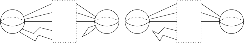
Figure 24. Front ($xz$) diagrams for Legendrian links $\Lambda,\Lambda^{\prime}$ in normal form related by Gompf move 4. The corners in these fronts are understood to be smoothed out.

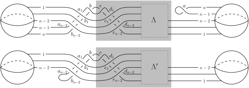
Figure 25. The $xy$ projections for $\Lambda$ and $\Lambda^{\prime}$ given in Figure 24, with some crossings labeled. The dotted boxes are identical (and correspond to the dotted boxes in Figure 24), as are the two shaded regions.

Let $\Lambda$ and $\Lambda^{\prime}$ be Legendrian links in $\#^{k}(S^{1}\times S^{2})$ related by Gompf move 4. Perturb the fronts of $\Lambda$ and $\Lambda^{\prime}$ to be in normal form, and then further perturb them to take the form shown in Figure 24. Then the corresponding $xy$ projections are in $xy$-normal form as shown in Figure 25.

By Proposition B.3, it suffices to show that the DGAs for $\Lambda$ and $\Lambda^{\prime}$ associated to the $xy$ projections shown in Figure 27 are stable tame isomorphic. Denote these DGAs by $(\mathcal{A},\partial)$ and $(\mathcal{A}^{\prime},\partial^{\prime})$ respectively. Note that we have labeled particular crossings in the $xy$ projections of $\Lambda$ and $\Lambda^{\prime}$; then $\mathcal{A}^{\prime}$ is generated by

• $c_{ij}^{p}$, $1\leq i,j\leq n-2$, and $p\geq 1$ if $i\geq j$

• $b,e,a_{1},\ldots,a_{n-2},b_{1},\ldots,b_{n-2},d_{1},\ldots,d_{n-2},e_{1},\ldots,e_{n-2}$

• the other “external” crossings contained in the dashed box in Figure 25,

while $\mathcal{A}$ is generated by the same generators along with

• $c_{ij}^{p}$, $1\leq i,j\leq n$, where at least one of $i,j$ is $n-1$ or $n$, and $p\geq 1$ if $i\geq j$

• $a$.

For the purpose of keeping track of signs, let $(m(1),\ldots,m(n))$ be the Maslov potential associated to strands $1,\ldots,n$ passing through the handle, and write $\sigma_{i}=(-1)^{m(i)}$ for each $i$. Note that $\sigma_{n-1}=-\sigma_{n}$, and if we write $\operatorname{sgn}(x)=(-1)^{|x|}$, then $\operatorname{sgn}(a)=-1$ and $\operatorname{sgn}(c_{ij}^{p})=-\sigma_{i}\sigma_{j}$.

Extend $\partial^{\prime}$ from $\mathcal{A}^{\prime}$ to $\mathcal{A}$ by setting

$$\partial^{\prime}(a) =1-c_{n-1,n}^{0},$$

$$\partial^{\prime}(c_{n-1,n}^{0}) =0,$$

$$\partial^{\prime}(c_{in}^{p}) =c_{i,n-1}^{p}, 1\leq i\leq n,~{}p\geq 1,\text{ if }i\geq n-1,$$

$$\partial^{\prime}(c_{i,n-1}^{p}) =0, 1\leq i\leq n,~{}p\geq 1\text{ if }i\geq n-1,$$

$$\partial^{\prime}(c_{n-1,j}^{p}) =c_{nj}^{p}, 1\leq j\leq n-2,~{}p\geq 1,$$

$$\partial^{\prime}(c_{nj}^{p}) =0, 1\leq j\leq n-2,~{}p\geq 1;$$

then $(\mathcal{A},\partial^{\prime})$ is a stabilization of $(\mathcal{A}^{\prime},\partial^{\prime})$. It suffices to construct a tame automorphism of $\mathcal{A}$ intertwining $\partial$ and $\partial^{\prime}$. To this end, we will construct elementary automorphisms $\Phi,\Psi,\Omega$ of $\mathcal{A}$ and establish that

(B.1) $$\partial\circ\Phi\circ\Psi\circ\Omega(x)=\Phi\circ\Psi\circ\Omega\circ\partial^{\prime}(x)$$

on generators $x$ of $\mathcal{A}$; then $\Phi\circ\Psi\circ\Omega$ is the desired tame automorphism.

We break down the generators of $\mathcal{A}$ into groups, and establish (B.1) for each group in turn:

• Group 1: $a$, $c_{n-1,n}^{0}$, $c_{ij}^{0}$ for $i,j\leq n-2$, and any crossing in the shaded regions in Figure 25 (including $e,e_{1},\ldots,e_{n-2},d_{1},\ldots,d_{n-2}$)

• Group 2: $c_{ij}^{p}$ for $p\geq 1$ and $i,j\leq n-2$

• Group 3: $c_{i,n-1}^{0}$ and $c_{in}^{0}$ where $i\leq n-2$, and $c_{ij}^{p}$ where $p\geq 1$ and either $i\geq n-1$ or $j\geq n-1$

• Group 4: $a_{1},\ldots,a_{n-2},b_{1},\ldots,b_{n-2},b$.

We will also present the definitions of $\Phi,\Psi,\Omega$ in turn as they are used. For now, we note that $\Phi,\Psi,\Omega$ will act as the identity on all generators of $\mathcal{A}$ except:

• for $\Phi$: Group 2

• for $\Psi$: Group 3

• for $\Omega$: Group 4.

If $x$ is in Group 1, then $\partial(x)=\partial^{\prime}(x)$; note in particular that this holds for $x=a$ and $x=c_{n-1,n}^{0}$ by the construction of $\partial^{\prime}$ and the fact (calculable from Figure 25) that $\partial(a)=1-c_{n-1,n}^{0}$. In addition, any generator appearing in this differential is also in Group 1. It follows that $\Phi\circ\Psi\circ\Omega$ acts as the identity on both $x$ and $\partial^{\prime}(x)$, and thus that (B.1) holds for $x$ in Group 1.

We next construct $\Phi$ so that (B.1) holds for $x$ in Group 2. First note that if $i,j\leq n-2$, then

$$\partial(c_{ij}^{p}) =\delta_{ij}\delta_{1p}+\sum_{m=1}^{n}\sum_{l=0}^{p}\sigma_{i}\sigma_{m}c_{im}^{l}c_{mj}^{p-l},$$

$$\partial^{\prime}(c_{ij}^{p}) =\delta_{ij}\delta_{1p}+\sum_{m=1}^{n-2}\sum_{l=0}^{p}\sigma_{i}\sigma_{m}c_{im}^{l}c_{mj}^{p-l}.$$

To define $\Phi$, we introduce some auxiliary elements of $\mathcal{A}$. We extend our definition of $c_{ij}^{p}$ to allow one or both of the indices $i,j$ to take the value $n-\text{\rm$\nicefrac{{1}}{{2}}$}$, as follows:

$$c_{n-\text{\rm$\nicefrac{{1}}{{2}}$},n}^{0} =c_{n-1,n-\text{\rm$\nicefrac{{1}}{{2}}$}}^{0}=1,$$

$$c_{n-\text{\rm$\nicefrac{{1}}{{2}}$},\alpha}^{p} =c_{n-1,\alpha}^{p}-ac_{n\alpha}^{p}, p\geq 1,~{}\alpha\in\{1,\ldots,n-1,n-\text{\rm$\nicefrac{{1}}{{2}}$},n\},$$

$$c_{\alpha,n-\text{\rm$\nicefrac{{1}}{{2}}$}}^{p} =c_{\alpha n}^{p}-c_{\alpha,n-1}^{p}a, p\geq 0\text{ and }\alpha\in\{1,\ldots,n-2\},$$

$$\text{or }p\geq 1\text{ and }\alpha\in\{n-1,n-\text{\rm$\nicefrac{{1}}{{2}}$},n\},$$

$$c_{\alpha\beta}^{0} =0, \alpha\geq\beta.$$

Note that the second and third lines overlap and agree in the definition of $c_{n-\text{\rm$\nicefrac{{1}}{{2}}$},n-\text{\rm$\nicefrac{{1}}{{2}}$}}^{p}$ for $p\geq 1$; in both cases, we find that

$$c_{n-\text{\rm$\nicefrac{{1}}{{2}}$},n-\text{\rm$\nicefrac{{1}}{{2}}$}}^{p}=c_{n-1,n}^{p}-c_{n-1,n-1}^{p}a-ac_{nn}^{p}+ac_{n,n-1}^{p}a.$$

Also define

$$\sigma_{n-\text{\rm$\nicefrac{{1}}{{2}}$}}=\sigma_{n-1}=-\sigma_{n}.$$

We collect a few facts about these new $c_{\alpha\beta}^{p}$ that are easy to verify from the definition.

Lemma B.6.

1. For $\alpha,\beta\in\{1,\ldots,n-1,n-\text{\rm$\nicefrac{{1}}{{2}}$},n\}$, $p_{2}>0$, and either $p_{1}>0$ or $p_{1}=0$ and $\alpha\geq n-2$, we have

   $$c_{\alpha,n-1}^{p_{1}}c_{n-1,n-\text{\rm$\nicefrac{{1}}{{2}}$}}^{0}c_{n-\text{\rm$\nicefrac{{1}}{{2}}$},\beta}^{p_{2}}-c_{\alpha,n-\text{\rm$\nicefrac{{1}}{{2}}$}}^{p_{1}}c_{n-\text{\rm$\nicefrac{{1}}{{2}}$},n}^{0}c_{n\beta}^{p_{2}}=c_{\alpha,n-1}^{p_{1}}c_{n-1,\beta}^{p_{2}}-c_{\alpha n}^{p_{1}}c_{n\beta}^{p_{2}}.$$

2. For $p\geq 0$ and $\alpha,\beta\in\{1,\ldots,n-1,n-\text{\rm$\nicefrac{{1}}{{2}}$},n\}$ with at least one of $\alpha,\beta=n-\text{\rm$\nicefrac{{1}}{{2}}$}$, we have

   $$\partial(c_{\alpha\beta}^{p})=\sum_{m=1}^{n}\sum_{l=0}^{p}\sigma_{\alpha}\sigma_{m}c_{\alpha m}^{l}c_{m\beta}^{p-l}$$

   where the sum on $m$ is only over integers.

Now define $\Phi:\thinspace\mathcal{A}\to\mathcal{A}$ as follows: $\Phi$ acts as the identity on all generators outside of Group 2, and if $p\geq 1$ and $i,j\leq n-2$, then

$$\Phi(c_{ij}^{p})=c_{ij}^{p}+\sum_{q\geq 1}(-1)^{q}\sum_{\lambda_{0}+\cdots+\lambda_{q}=p+1}c_{i,n-\text{\rm$\nicefrac{{1}}{{2}}$}}^{\lambda_{0}-1}c_{n-\text{\rm$\nicefrac{{1}}{{2}}$},n-\text{\rm$\nicefrac{{1}}{{2}}$}}^{\lambda_{1}}\cdots c_{n-\text{\rm$\nicefrac{{1}}{{2}}$},n-\text{\rm$\nicefrac{{1}}{{2}}$}}^{\lambda_{q-1}}c_{n-\text{\rm$\nicefrac{{1}}{{2}}$},j}^{\lambda_{q}},$$

where the second sum is over all ways to write $p+1=\lambda_{0}+\cdots+\lambda_{q}$ for any $\lambda_{0},\ldots,\lambda_{q}\geq 1$. For example, for $i,j\leq n-2$,

$$\Phi(c_{ij}^{1}) =c_{ij}^{1}-c_{i,n-\text{\rm$\nicefrac{{1}}{{2}}$}}^{0}c_{n-\text{\rm$\nicefrac{{1}}{{2}}$},j}^{1},$$

$$\Phi(c_{ij}^{2}) =c_{ij}^{2}-c_{i,n-\text{\rm$\nicefrac{{1}}{{2}}$}}^{0}c_{n-\text{\rm$\nicefrac{{1}}{{2}}$},j}^{2}-c_{i,n-\text{\rm$\nicefrac{{1}}{{2}}$}}^{1}c_{n-\text{\rm$\nicefrac{{1}}{{2}}$},j}^{1}+c_{i,n-\text{\rm$\nicefrac{{1}}{{2}}$}}^{0}c_{n-\text{\rm$\nicefrac{{1}}{{2}}$},n-\text{\rm$\nicefrac{{1}}{{2}}$}}^{1}c_{n-\text{\rm$\nicefrac{{1}}{{2}}$},j}^{1}.$$

Choose any ordering of $\mathcal{A}$ for which the $c_{ij}^{p}$ generators are ordered so that $c_{ij}^{p}<c_{i^{\prime}j^{\prime}}^{p}$ whenever $np+j-i<np^{\prime}+j^{\prime}-i^{\prime}$. With respect to the induced filtration on $\mathcal{A}$, the differentials $\partial$ and $\partial^{\prime}$ are filtered, sending $c_{ij}^{p}$ to a sum of terms lower in the filtration. It is then easy to check that $\Phi$ is elementary with respect to this ordering.

We can now establish (B.1) for $x$ in Group 2. This is a result of the following lemma, along with the fact that the differential $\partial^{\prime}$, applied to a generator in Group 2, only involves generators in Groups 1 and 2.

Lemma B.7.

For all $p\geq 0$ and all $i,j\leq n-2$,

$$\partial\circ\Phi(c_{ij}^{p})=\Phi\circ\partial^{\prime}(c_{ij}^{p}).$$

Proof.

We have

$$\Phi\circ\partial^{\prime}(c_{ij}^{p})=\sum_{m\leq n-2}\sum_{l}\sigma_{i}\sigma_{m}\Phi(c_{im}^{l})\Phi(c_{mj}^{p-l})+\delta_{ij}\delta_{1p}.$$

When we expand this out using the definition of $\Phi$, besides $\delta_{ij}\delta_{1p}$, we obtain a sum of terms of the form

$$\sigma_{i}\sigma_{m}(-1)^{q}c_{i,n-\text{\rm$\nicefrac{{1}}{{2}}$}}\cdots c_{n-\text{\rm$\nicefrac{{1}}{{2}}$},m}c_{m,n-\text{\rm$\nicefrac{{1}}{{2}}$}}\cdots c_{n-\text{\rm$\nicefrac{{1}}{{2}}$},j}$$

with $m\leq n-2$, where we have suppressed the superscripts on the $c$’s, and $q$ is the length of the word $c_{i,n-\text{\rm$\nicefrac{{1}}{{2}}$}}\cdots c_{n-\text{\rm$\nicefrac{{1}}{{2}}$},m}c_{m,n-\text{\rm$\nicefrac{{1}}{{2}}$}}\cdots c_{n-\text{\rm$\nicefrac{{1}}{{2}}$},j}$. (Some terms are shorter than this, e.g., $\sigma_{i}\sigma_{m}(-1)^{q}c_{im}c_{m,n-\text{\rm$\nicefrac{{1}}{{2}}$}}\cdots c_{n-\text{\rm$\nicefrac{{1}}{{2}}$},j}$, but the following argument still applies.) Note that this term also appears, with the same sign, in $\partial((-1)^{q}c_{i,n-\text{\rm$\nicefrac{{1}}{{2}}$}}\cdots c_{n-\text{\rm$\nicefrac{{1}}{{2}}$},n-\text{\rm$\nicefrac{{1}}{{2}}$}}\cdots c_{n-\text{\rm$\nicefrac{{1}}{{2}}$},j})$, where $q-1$ is the length of the word $c_{i,n-\text{\rm$\nicefrac{{1}}{{2}}$}}\cdots c_{n-\text{\rm$\nicefrac{{1}}{{2}}$},n-\text{\rm$\nicefrac{{1}}{{2}}$}}\cdots c_{n-\text{\rm$\nicefrac{{1}}{{2}}$},j})$, by Lemma B.6(2) and the fact that $\operatorname{sgn}(c_{i,n-\text{\rm$\nicefrac{{1}}{{2}}$}})=-\sigma_{i}\sigma_{n}$ and $\operatorname{sgn}(c_{n-\text{\rm$\nicefrac{{1}}{{2}}$},n-\text{\rm$\nicefrac{{1}}{{2}}$}})=1$. Thus every term in the expansion of $\Phi\circ\partial^{\prime}(c_{ij}^{p})$ has a corresponding term in the expansion of $\partial\circ\Phi(c_{ij}^{p})$ (and this also holds for the extra term $\delta_{ij}\delta_{1p}$).

It suffices to check that the sum $S$ of the remaining terms in the expansion of $\partial\circ\Phi(c_{ij}^{p})=\partial(\sum(\pm c_{i,n-\text{\rm$\nicefrac{{1}}{{2}}$}}\cdots c_{n-\text{\rm$\nicefrac{{1}}{{2}}$},j}))$ is $0$. These are the terms for which, besides $i$ at the beginning and $j$ at the end, no subscripts $\leq n-2$ appear. We can write $S$ as a finite sum $S_{1}+S_{2}+\cdots$, where $S_{1}$ is the contribution of $\partial(c_{ij}^{p})$, $S_{2}$ is the contribution of $\partial(-\sum c_{i,n-\text{\rm$\nicefrac{{1}}{{2}}$}}c_{n-\text{\rm$\nicefrac{{1}}{{2}}$},j})$, and so forth. More precisely, we have

$$S_{1} =\sigma_{i}\sigma_{n-1}\sum_{\lambda_{0}+\lambda_{1}=p+1}(c_{i,n-1}^{\lambda_{0}-1}c_{n-1,j}^{\lambda_{1}}-c_{in}^{\lambda_{0}-1}c_{nj}^{\lambda_{1}}),$$

$$S_{2} =-\sigma_{i}\sigma_{n-1}\sum_{\lambda_{0}+\lambda_{1}+\lambda_{2}=p+1}\left(c_{i,n-1}^{\lambda_{0}-1}c_{n-1,n-\text{\rm$\nicefrac{{1}}{{2}}$}}^{\lambda_{1}}c_{n-\text{\rm$\nicefrac{{1}}{{2}}$},j}^{\lambda_{2}}-c_{in}^{\lambda_{0}-1}c_{n,n-\text{\rm$\nicefrac{{1}}{{2}}$}}^{\lambda_{1}}c_{n-\text{\rm$\nicefrac{{1}}{{2}}$},j}^{\lambda_{2}}\right.$$

$$\qquad\qquad\qquad\qquad\qquad\left.+c_{i,n-\text{\rm$\nicefrac{{1}}{{2}}$}}^{\lambda_{0}-1}c_{n-\text{\rm$\nicefrac{{1}}{{2}}$},n-1}^{\lambda_{1}}c_{n-1,j}^{\lambda_{2}}-c_{i,n-\text{\rm$\nicefrac{{1}}{{2}}$}}^{\lambda_{0}-1}c_{n-\text{\rm$\nicefrac{{1}}{{2}}$},n}^{\lambda_{1}}c_{nj}^{\lambda_{2}}\right)$$

and so forth, where all sums are over $\lambda_{0}\geq 1$ and $\lambda_{i}\geq 0$ for $i\geq 1$. Each nonzero term in these sums either has all $\lambda_{q}\geq 1$, or it has exactly one $\lambda_{q}=0$ (where $q>0$) and incorporates either $c_{n-1,n-\text{\rm$\nicefrac{{1}}{{2}}$}}^{0}$ or $c_{n-\text{\rm$\nicefrac{{1}}{{2}}$},n}^{0}$. We can then write $S_{r}=S_{r}^{0}+S_{r}^{1}$, where $S_{r}^{0}$ sums the terms with some $\lambda_{q}=0$, and $S_{r}^{1}$ sums the terms with all $\lambda_{q}\geq 1$.

Note that $S_{1}^{0}=0$ and $S_{1}^{1}=S_{1}$, while

$$S_{2}^{0} =-\sigma_{i}\sigma_{n-1}\sum_{\lambda_{0}+\lambda_{2}=p+1}\left(c_{i,n-1}^{\lambda_{0}-1}c_{n-1,n-\text{\rm$\nicefrac{{1}}{{2}}$}}^{0}c_{n-\text{\rm$\nicefrac{{1}}{{2}}$},j}^{\lambda_{2}}-c_{i,n-\text{\rm$\nicefrac{{1}}{{2}}$}}^{\lambda_{0}-1}c_{n-\text{\rm$\nicefrac{{1}}{{2}}$},n}^{0}c_{nj}^{\lambda_{2}}\right)$$

$$=-\sigma_{i}\sigma_{n-1}\sum_{\lambda_{0}+\lambda_{2}=p+1}\left(c_{i,n-1}^{\lambda_{0}-1}c_{n-1,j}^{\lambda_{2}}-c_{in}^{\lambda_{0}-1}c_{nj}^{\lambda_{2}}\right)$$

$$=-S_{1}^{1},$$

where the middle equality follows from Lemma B.6(1). Similarly $S_{r}^{0}=-S_{r-1}^{1}$ for all $r\geq 2$, whence $S=\sum_{r}(S_{r}^{0}+S_{r}^{1})=0$. ∎

We next turn our attention to the definition of $\Psi$ and establishing (B.1) for Group 3 generators. First define the differential $\partial^{\prime\prime}:\thinspace\mathcal{A}\to\mathcal{A}$ by $\partial^{\prime\prime}=\Phi^{-1}\circ\partial\circ\Phi$. For any $1\leq i\leq n$ and $p\geq 0$, we have

$$\partial^{\prime\prime}(c_{in}^{p}) =\Phi^{-1}\partial\Phi(c_{in}^{p})=\Phi^{-1}\partial(c_{in}^{p})$$

$$=\Phi^{-1}(\sigma_{i}\sigma_{n-1}c_{i,n-1}^{p}c_{n-1,n}^{0}+\cdots)=\sigma_{i}\sigma_{n-1}c_{i,n-1}^{p}c_{n-1,n}^{0}+\cdots,$$

where the ellipses involve only terms lower than $c_{i,n-1}^{p}$ in the filtration chosen earlier. Denote the final ellipsis by

$$\partial^{\prime\prime}_{0}(c_{in}^{p}):=\partial^{\prime\prime}(c_{in}^{p})-\sigma_{i}\sigma_{n-1}c_{i,n-1}^{p}c_{n-1,n}^{0}.$$

Similarly, for any $1\leq j\leq n-2$ and $p\geq 1$, we can define $\partial^{\prime\prime}_{0}(c_{n-1,j}^{p})$ by

$$\partial^{\prime\prime}_{0}(c_{n-1,j}^{p}):=\partial^{\prime\prime}(c_{n-1,j}^{p})+c_{n-1,n}^{0}c_{nj}^{p},$$

and $\partial^{\prime\prime}_{0}(c_{n-1,j}^{p})$ is lower in the filtration than $c_{nj}^{p}$.

Now define the algebra map $\Psi:\thinspace\mathcal{A}\to\mathcal{A}$ by

$$\Psi(c_{i,n-1}^{p}) =\sigma_{i}\sigma_{n-1}c_{i,n-1}^{p}+\partial^{\prime\prime}_{0}(c_{in}^{p})+\partial^{\prime\prime}(c_{i,n-1}^{p})a p\geq 1\text{ and }1\leq i\leq n,$$

$$\text{or }p=0\text{ and }i\leq n-2$$

$$\Psi(c_{in}^{p}) =c_{in}^{p}-c_{i,n-1}^{p}a p\geq 1\text{ and }1\leq i\leq n,$$

$$\text{or }p=0\text{ and }i\neq n-2,$$

$$\Psi(c_{nj}^{p}) =-c_{nj}^{p}+\partial^{\prime\prime}_{0}(c_{n-1,j}^{p})+a\partial^{\prime\prime}(c_{nj}^{p}) p\geq 1\text{ and }1\leq j\leq n-2$$

$$\Psi(c_{n-1,j}^{p}) =c_{n-1,j}^{p}-ac_{nj}^{p} p\geq 1\text{ and }1\leq j\leq n-2$$

and $\Psi$ acts as the identity on all other generators of $\mathcal{A}$. From the above discussion, $\Psi$ is elementary with respect to the chosen ordering on $\mathcal{A}$.

Lemma B.8.

If $x$ is a generator in Group 3, then

$$\partial^{\prime\prime}\circ\Psi(x)=\Psi\circ\partial^{\prime}(x).$$

Proof.

If either $p\geq 1$ or $p=0$ and $i\leq n-2$, we have

$$\partial^{\prime\prime}\Psi(c_{in}^{p}) =\partial^{\prime\prime}(c_{in}^{p}-c_{i,n-1}^{p}a)$$

$$=(\sigma_{i}\sigma_{n-1}c_{i,n-1}^{p}c_{n-1,n}^{0}+\partial^{\prime\prime}_{0}(c_{in}^{p}))$$

$$+(\partial^{\prime\prime}(c_{i,n-1}^{p})a-\sigma_{i}\sigma_{n-1}c_{i,n-1}^{p}(1+c_{n-1,n}^{0}))$$

$$=\Psi(c_{i,n-1}^{p})$$

$$=\Psi\partial^{\prime}(c_{in}^{p})$$

whence $\partial^{\prime\prime}\Psi(c_{i,n-1}^{p})=(\partial^{\prime\prime})^{2}\Psi(c_{in}^{p})=0=\Psi\partial^{\prime}(c_{i,n-1}^{p})$, and the lemma holds for $x=c_{in}^{p}$ and $x=c_{i,n-1}^{p}$. If $p\geq 1$ and $j\leq n-2$, then a similar calculation yields $\partial^{\prime\prime}\Psi(c_{n-1,j}^{p})=\Psi\partial^{\prime}(c_{n-1,j}^{p})$ and $\partial^{\prime\prime}\Psi(c_{nj}^{p})=0=\Psi\partial^{\prime}(c_{nj}^{p})$, and the lemma holds for $x=c_{n-1,j}^{p}$ and $x=c_{nj}^{p}$. ∎

It follows immediately from Lemma B.8 that (B.1) holds when $x$ is a Group 3 generator, since then $\partial\Phi\Psi\Omega(x)=\partial\Phi\Psi(x)=\Phi\partial^{\prime\prime}\Psi(x)=\Phi\Psi\partial^{\prime}(x)=\Phi\Psi\Omega\partial^{\prime}(x)$.

Finally, it remains to define $\Omega$ and establish (B.1) for Group 4 generators. Define the algebra map $\Omega:\thinspace\mathcal{A}\to\mathcal{A}$ by

$$\Omega(a_{i}) =a_{i}-\sigma_{i}\sigma_{n-1}c_{in}^{0}, 1\leq i\leq n-2,$$

$$\Omega(b_{i}) =b_{i}+a_{i}a, 1\leq i\leq n-2,$$

$$\Omega(b) =b+a,$$

and $\Omega$ is the identity on all other generators of $\mathcal{A}$. We can choose an ordering of $\mathcal{A}$ (independently from before) such that $a<b$ and $c_{in}^{0}a<a_{i}<b_{i}$ for all $1\leq i\leq n-2$; then $\Omega$ is elementary with respect to this ordering.

An inspection of Figure 25 yields, for $i\leq n-2$:

$$\partial(a_{i}) =\sum_{j=i+1}^{n-2}c_{ij}^{0}a_{j}+c_{i,n-1}^{0}-\sigma_{i}\sigma_{n-1}d_{i},$$

$$\partial^{\prime}(a_{i}) =\sum_{j=i+1}^{n-2}c_{ij}^{0}a_{j}-\sigma_{i}\sigma_{n-1}d_{i},$$

$$\partial(b_{i}) =\sum_{j=i+1}^{n-2}c_{ij}^{0}b_{j}+c_{in}^{0}-\sigma_{i}\sigma_{n-1}a_{i}c_{n-1,n}^{0}-\sigma_{i}\sigma_{n}e_{i}-\sigma_{i}\sigma_{n}d_{i}b,$$

$$\partial^{\prime}(b_{i}) =\sum_{j=i+1}^{n-2}c_{ij}^{0}b_{j}-\sigma_{i}\sigma_{n-1}a_{i}-\sigma_{i}\sigma_{n}e_{i}-\sigma_{i}\sigma_{n}d_{i}b,$$

$$\partial(b) =e+c_{n-1,n}^{0},$$

$$\partial^{\prime}(b) =e+1.$$

Note in particular that there are no holomorphic disks whose only positive puncture is at $a_{i}$ or $b_{i}$ and extend into the dotted boxes in Figure 25. This can be shown in general via an area estimate, or more simply by assuming that the figures in the dotted boxes are the result of resolution, in which case the rightmost point in such a holomorphic disk would have to be a positive puncture (cf. the differential for simple fronts in [27]).

One can now check directly that (B.1) holds for generators in Group 4, i.e., $a_{i}$, $b_{i}$, and $b$. For instance, from the definition of $\Psi$, we have $\Psi(c_{in}^{0})=c_{in}^{0}-c_{i,n-1}^{0}a$, and thus

$$\partial\Phi\Psi\Omega(a_{i}) =\partial\Phi\Psi(a_{i}-\sigma_{i}\sigma_{n-1}c_{in}^{0})$$

$$=\partial(a_{i}-\sigma_{i}\sigma_{n-1}(c_{in}^{0}-c_{i,n-1}^{0}a))$$

$$=-\sigma_{i}\sigma_{n-1}d_{i}+\sum_{j=i+1}^{n-2}c_{ij}(a_{j}-\sigma_{j}\sigma_{n-1}(c_{jn}^{0}-c_{j,n-1}^{0}a))$$

$$=\Phi\Psi(-\sigma_{i}\sigma_{n-1}d_{i}+\sum_{j=i+1}^{n-2}c_{ij}(a_{j}-\sigma_{j}\sigma_{n-1}c_{jn}^{0}))$$

$$=\Phi\Psi\Omega(-\sigma_{i}\sigma_{n-1}d_{i}+\sum_{j=i+1}^{n-2}c_{ij}^{0}a_{j})$$

$$=\Phi\Psi\Omega\partial^{\prime}(a_{i}).$$

Similar computations hold for $b_{i}$ and $b$.

This completes the proof of (B.1) for all generators of $\mathcal{A}$, and the proof of invariance under Gompf move 4.

B.2.E. Invariance under Gompf move 5

Proposition B.9.

If $\Lambda$ and $\Lambda^{\prime}$ are Legendrian links in $\#^{k}(S^{1}\times S^{2})$ in normal form, related by Gompf move 5, then the DGAs associated to $\pi_{xy}(\Lambda)$ and $\pi_{xy}(\Lambda^{\prime})$ are stable tame isomorphic.

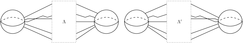
Figure 26. Front ($xz$) diagrams for Legendrian links $\Lambda,\Lambda^{\prime}$ in normal form related by Gompf move 5. The corners in these fronts are understood to be smoothed out.

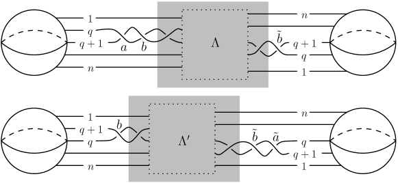
Figure 27. The $xy$ projections for $\Lambda$ and $\Lambda^{\prime}$ given in Figure 26. The dotted boxes are identical (and correspond to the dotted boxes in Figure 26), as are the two shaded regions. Note the unusual labeling of strands in the $xy$ projection of $\Lambda^{\prime}$: $q$ and $q+1$ are switched.

Let $\Lambda$ and $\Lambda^{\prime}$ be Legendrian links in $\#^{k}(S^{1}\times S^{2})$ related by Gompf move 5. Perturb the fronts of $\Lambda$ and $\Lambda^{\prime}$ to be in normal form, and then further perturb them to take the form shown in Figure 26. Then the corresponding $xy$ projections are in $xy$-normal form as shown in Figure 27.

By Proposition B.3, it suffices to show that the DGAs for $\Lambda$ and $\Lambda^{\prime}$ associated to the $xy$ projections shown in Figure 27 are stable tame isomorphic. Denote these DGAs by $(\mathcal{A},\partial)$ and $(\mathcal{A}^{\prime},\partial^{\prime})$ respectively. (Note that we have labeled particular crossings $a,b,\tilde{b}$ in $\pi_{xy}(\Lambda)$ and $\tilde{a},b,\tilde{b}$ in $\pi_{xy}(\Lambda^{\prime})$.)

The generator sets for $\mathcal{A}$ and $\mathcal{A}^{\prime}$ are identical, except that $a$ and $c_{q,q+1}^{0}$ are generators for $\mathcal{A}$ but not $\mathcal{A}^{\prime}$, and $\tilde{a}$ and $c_{q+1,q}^{0}$ are generators for $\mathcal{A}^{\prime}$ but not $\mathcal{A}$. Note that the presence of $c_{q+1,q}^{0}$ rather than $c_{q,q+1}^{0}$ in $\mathcal{A}^{\prime}$ is due to the switching of labels $q$ and $q+1$ in the bottom diagram of Figure 27. As for grading, the strands passing through the $1$-handle in $\pi_{xy}(\Lambda)$ and $\pi_{xy}(\Lambda^{\prime})$ share a common Maslov potential $(m(1),\ldots,m(n))$, with $m(i)$ being the potential for the strand labeled $i$, and it follows that all common generators of $\mathcal{A}$ and $\mathcal{A}^{\prime}$ have the same grading in both. For future reference, write $\sigma_{i}=(-1)^{m(i)}$ and note that

(B.2) $$\operatorname{sgn}a=\operatorname{sgn}\tilde{a}=\operatorname{sgn}b=\operatorname{sgn}\tilde{b}=-\operatorname{sgn}c_{q,q+1}^{0}=-\operatorname{sgn}c_{q+1,q}^{0}=\sigma_{q}\sigma_{q+1}$$

where $\operatorname{sgn}a=(-1)^{|a|}$, etc.

Define $\tilde{\mathcal{A}}$ to be the graded tensor algebra generated by the union of the sets of generators of $\mathcal{A}$ and $\mathcal{A}^{\prime}$. We can extend the differential $\partial$ from $\mathcal{A}$ to $\tilde{\mathcal{A}}$, and $\partial^{\prime}$ from $\mathcal{A}^{\prime}$ to $\tilde{\mathcal{A}}$, by setting

$$\partial(\tilde{a}) =-c_{q+1,q}^{0}, \partial(c_{q+1,q}^{0}) =0,$$

$$\partial^{\prime}(a) =c_{q,q+1}^{0}, \partial^{\prime}(c_{q,q+1}^{0}) =0.$$

Then $(\tilde{\mathcal{A}},\partial)$ is a stabilization of $(\mathcal{A},\partial)$, $(\tilde{\mathcal{A}},\partial^{\prime})$ is a stabilization of $(\mathcal{A}^{\prime},\partial^{\prime})$, and it suffices to show that $(\tilde{\mathcal{A}},\partial)$ and $(\tilde{\mathcal{A}},\partial^{\prime})$ are tamely isomorphic.

Define an algebra automorphism $\Phi$ of $\tilde{\mathcal{A}}$ as follows:

$$\Phi(b) =b-\tilde{a}$$

$$\Phi(c_{qj}^{p}) =c_{qj}^{p}-\sigma_{q}\sigma_{q+1}ac_{q+1,j}^{p}, j\neq q+1;~{}p\geq 1\text{ if }j\leq q,$$

$$\Phi(c_{i,q+1}^{p}) =c_{i,q+1}^{p}+c_{iq}^{p}a, i\neq q;~{}p\geq 1\text{ if }i\geq q+1,$$

$$\Phi(c_{q,q+1}^{p}) =c_{q,q+1}^{p}+c_{qq}^{p}a$$

$$-\sigma_{q}\sigma_{q+1}(ac_{q+1,q+1}^{p}+ac_{q+1,q}^{p}a), p\geq 1,$$

and $\Phi$ acts as the identity on all other generators of $\tilde{\mathcal{A}}$. (In particular, $\Phi(c_{q,q+1}^{0})=c_{q,q+1}^{0}$ and $\Phi(c_{q+1,q}^{0})=c_{q+1,q}^{0}$.) It is easy to check that $\Phi$ is elementary: choose any ordering such that $a,\tilde{a}$ are at the bottom and for fixed $p$, the $c_{ij}^{p}$ are ordered so that $c_{ij}^{p}<c_{i^{\prime}j^{\prime}}^{p}$ if $j-i<j^{\prime}-i^{\prime}$. Similarly, define an elementary automorphism $\Phi^{\prime}$ of $\tilde{\mathcal{A}}$ by

$$\Phi^{\prime}(\tilde{b}) =\tilde{b}-a$$

$$\Phi^{\prime}(c_{q+1,j}^{p}) =c_{q+1,j}^{p}+\sigma_{q}\sigma_{q+1}\tilde{a}c_{qj}^{p} j\neq q;~{}p\geq 1\text{ if }j\leq q+1$$

$$\Phi^{\prime}(c_{iq}^{p}) =c_{iq}^{p}-c_{i,q+1}^{p}\tilde{a} i\neq q+1;~{}p\geq 1\text{ if }i\geq q$$

$$\Phi^{\prime}(c_{q+1,q}^{p}) =c_{q+1,q}^{p}-c_{q+1,q+1}^{p}\tilde{a}$$

$$+\sigma_{q}\sigma_{q+1}(\tilde{a}c_{qq}^{p}-\tilde{a}c_{q,q+1}^{p}\tilde{a}) p\geq 1,$$

and $\Phi^{\prime}$ acts as the identity on all other generators of $\tilde{\mathcal{A}}$.

To complete the proof of invariance for Gompf move 5, we will establish that

(B.3) $$\Phi^{-1}\circ\partial\circ\Phi=(\Phi^{\prime})^{-1}\circ\partial^{\prime}\circ\Phi^{\prime}$$

on $\tilde{\mathcal{A}}$. It suffices to establish (B.3) on generators of $\tilde{\mathcal{A}}$, which we divide into groups: $a,b,\tilde{a},\tilde{b}$; internal generators $c_{ij}^{p}$, including $c_{q,q+1}^{0}$ and $c_{q+1,q}^{0}$; and external generators, which correspond to crossings in the shaded regions of Figure 27. For $a,b,\tilde{a},\tilde{b}$, note that $\partial(a)=c_{q,q+1}^{0}$, $\partial(b)=x$, and $\partial^{\prime}(b)=c_{q+1,q}^{0}+x$, where $x$ only involves external generators (in fact, up to sign, $x$ is just the external generator corresponding to the leftmost crossing in the shaded region), and so $\Phi^{-1}\partial\Phi a=c_{q,q+1}^{0}=(\Phi^{\prime})^{-1}\partial^{\prime}\Phi^{\prime}a$ and

$$\Phi^{-1}\partial\Phi b =\Phi^{-1}\partial(b-\tilde{a})=\Phi^{-1}(x+c_{q+1,q}^{0})$$

$$=x+c_{q+1,q}^{0}=(\Phi^{\prime})^{-1}(x+c_{q+1,q}^{0})=(\Phi^{\prime})^{-1}\partial^{\prime}\Phi^{\prime}b.$$

Similarly, (B.3) holds for $\tilde{a}$ and $\tilde{b}$.

Next, we check (B.3) for internal generators $c_{ij}^{p}$. Let $\pi:\thinspace\tilde{\mathcal{A}}\to\tilde{\mathcal{A}}$ be the algebra map that sends $c_{q,q+1}^{0}$ and $c_{q+1,q}^{0}$ to $0$ and acts as the identity on all other generators of $\tilde{\mathcal{A}}$. Since the internal differentials $\partial$ and $\partial^{\prime}$ only differ in terms that involve either $c_{q,q+1}^{0}$ and $c_{q+1,q}^{0}$, we have $\pi\partial c_{ij}^{p}=\pi\partial^{\prime}c_{ij}^{p}$ for all $i,j,p$. Equation (B.3) for internal generators is the content of the following result.

Lemma B.10.

For all $i,j,p$, we have

$$\Phi^{-1}\partial\Phi(c_{ij}^{p})=\pi\partial c_{ij}^{p}=\pi\partial^{\prime}c_{ij}^{p}=(\Phi^{\prime})^{-1}\partial^{\prime}\Phi^{\prime}(c_{ij}^{p}).$$

Proof.

We will show that $\Phi^{-1}\partial\Phi(c_{ij}^{p})=\pi\partial c_{ij}^{p}$; the proof that $(\Phi^{\prime})^{-1}\partial^{\prime}\Phi^{\prime}(c_{ij}^{p})=\pi\partial^{\prime}c_{ij}^{p}$ is essentially identical. We first establish this when $i\neq q$ and $j\neq q+1$. In this case, from the definition of $\Phi$, we have

$$\Phi(\sigma_{i}\sigma_{q}c_{iq}^{l}c_{qj}^{p-l}+\sigma_{i}\sigma_{q+1}c_{i,q+1}^{l}c_{q+1,j}^{p-l})=\sigma_{i}\sigma_{q}c_{iq}^{l}c_{qj}^{p-l}+\sigma_{i}\sigma_{q+1}c_{i,q+1}^{l}c_{q+1,j}^{p-l},$$

whence $\Phi(\partial c_{ij}^{p})=\partial c_{ij}^{p}$. Thus

$$\Phi^{-1}\partial\Phi(c_{ij}^{p})=\Phi^{-1}\partial c_{ij}^{p}=\partial c_{ij}^{p}=\pi\partial c_{ij}^{p},$$

where the last equality follows from the fact that $c_{q,q+1}^{0}$ does not appear in $\partial c_{ij}^{p}$.

It remains to prove the lemma when $i=q$ or $j=q+1$. This breaks into three cases: $i=q$ and $j\neq q+1$, $i\neq q$ and $j=q+1$, and $i=q$ and $j=q+1$. We will establish the first case and leave the similar calculations for the other two cases to the reader. For $j\neq q+1$, we have

$$\Phi\pi\partial(c_{qj}^{p}) =\delta_{qj}\delta_{1p}+\sum_{(m,l)\neq(q+1,0)}\sigma_{q}\sigma_{m}\Phi(c_{qm}^{l})\Phi(c_{mj}^{p-l})$$

$$=\delta_{qj}\delta_{1p}+\sum_{(m,l)\neq(q+1,0)}\sigma_{q}\sigma_{m}(c_{qm}^{l}-\sigma_{q}\sigma_{q+1}ac_{q+1,m}^{l})c_{mj}^{p-l}$$

$$\quad+\sum_{l>0}(c_{qq}^{l}-\sigma_{q}\sigma_{q+1}ac_{q+1,q}^{l})(-\sigma_{q}\sigma_{q+1}ac_{q+1,j}^{p-l})$$

$$\quad+\sum_{l>0}\sigma_{q}\sigma_{q+1}(c_{qq}^{l}a-\sigma_{q}\sigma_{q+1}ac_{q+1,q}^{p-l}a)c_{q+1,j}^{p-l}$$

$$=\delta_{qj}\delta_{1p}+\sum_{(m,l)\neq(q+1,0)}\sigma_{q}\sigma_{m}(c_{qm}^{l}-\sigma_{q}\sigma_{q+1}ac_{q+1,m}^{l})c_{mj}^{p-l}$$

$$=\delta_{qj}\delta_{1p}+\sum_{m,l}\sigma_{q}\sigma_{m}c_{qm}^{l}c_{mj}^{p-l}-\sigma_{q}\sigma_{q+1}c_{q,q+1}^{0}c_{q+1,j}^{p}$$

$$\quad-\sum_{m,l}\sigma_{q+1}\sigma_{m}ac_{q+1,m}^{l}c_{mj}^{p-l}$$

$$=\partial(c_{qj}^{p}-\sigma_{q}\sigma_{q+1}ac_{q+1,j}^{p})$$

$$=\partial\Phi(c_{qj}^{p}),$$

where the second and third sums after the second equality arise from the fact that $\Phi(c_{mj}^{p-l})$ and $\Phi(c_{qm}^{l})$ have additional terms when $m=q$ and $m=q+1$, respectively. Thus $\Phi^{-1}\partial\Phi(c_{qj}^{p})=\pi\partial c_{qj}^{p}$, as desired. ∎

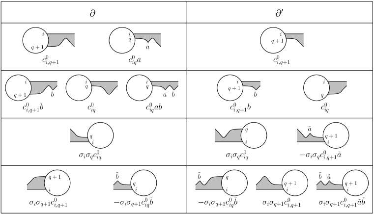
Figure 28. Disks contributing to the differentials $\partial x$ or $\partial^{\prime}x$ and involving $c_{iq}^{0},c_{i,q+1}^{0}$ for $i<q$, arranged into families; the depicted portions are the parts outside the shaded region in Figure 27. Some of these disks also have negative corners at $a$, $\tilde{a}$, $b$, or $\tilde{b}$, as shown. Circles represent the handle $2$-spheres. The positive corner $x$ is not shown but is to the right of each diagram where the $2$-sphere is on the left, and vice versa. The words underneath each disk are the contributions of the depicted portion of the disk to the corresponding word in $\partial$ or $\partial^{\prime}$. Orientation signs are calculated from the rules in Section 2.4, with some simplification due to (B.2).

Finally, we need to check (B.3) for external generators, corresponding to crossings in the shaded region of Figure 27. Let $x$ be such a crossing; we need to show that $\Phi^{-1}\partial x=(\Phi^{\prime})^{-1}\partial^{\prime}x$. The only generators appearing in $\partial x$ or $\partial^{\prime}x$ that are affected by $\Phi$ or $\Phi^{\prime}$ are $b$, $\tilde{b}$, and generators of the form $c_{iq}^{0},c_{i,q+1}^{0}$ for $i<q$ and $c_{qj}^{0},c_{q+1,j}^{0}$. The terms in $\partial x$ and $\partial^{\prime}x$ that do not include any of these generators are identical, while the terms that do include these generators can be grouped as shown in Figure 28 (which shows terms involving $c_{iq}^{0}$ or $c_{i,q+1}^{0}$ for $i<q$; there is an entirely analogous group of diagrams for terms involving $c_{qj}^{0}$ or $c_{q+1,j}^{0}$ for $j>q+1$). For instance, the top left set of diagrams corresponds to a collection of terms $y(c_{i,q+1}^{0}+c_{iq}^{0}a)z$ in $\partial x$ and a term $yc_{i,q+1}^{0}z$ in $\partial^{\prime}x$. The fact that $\Phi^{-1}\partial x=(\Phi^{\prime})^{-1}\partial^{\prime}x$ now follows from the following identities, easily checked from the definitions of $\Phi$ and $\Phi^{\prime}$:

$$\Phi^{-1}(c_{i,q+1}^{0}+c_{iq}^{0}a) =(\Phi^{\prime})^{-1}(c_{i,q+1}^{0})=c_{i,q+1}^{0}$$

$$\Phi^{-1}(c_{iq}^{0}+c_{i,q+1}^{0}b+c_{iq}^{0}ab) =(\Phi^{\prime})^{-1}(c_{iq}^{0}+c_{i,q+1}^{0}b)=c_{iq}^{0}+c_{i,q+1}^{0}(b+\tilde{a})$$

$$\Phi^{-1}(c_{iq}^{0}) =(\Phi^{\prime})^{-1}(c_{iq}^{0}-c_{i,q+1}^{0}\tilde{a})=c_{iq}^{0}$$

$$\Phi^{-1}(c_{i,q+1}^{0}-c_{iq}^{0}\tilde{b}) =(\Phi^{\prime})^{-1}(c_{i,q+1}^{0}-c_{iq}^{0}\tilde{b}+c_{i,q+1}^{0}\tilde{a}\tilde{b})$$

$$=c_{i,q+1}^{0}-c_{iq}^{0}(a+\tilde{b}),$$

along with the analogous identities involving $c_{qj}^{0}$ and $c_{q+1,j}^{0}$.

B.2.F. Invariance under Gompf move 6, part 1

Proposition B.11.

If $\Lambda$ and $\Lambda^{\prime}$ are Legendrian links in $\#^{k}(S^{1}\times S^{2})$ in normal form, related by Gompf move 6, then the DGAs associated to $\pi_{xy}(\Lambda)$ and $\pi_{xy}(\Lambda^{\prime})$ are stable tame isomorphic.

The proof of Proposition B.11 occupies this section and the following section B.2.G.

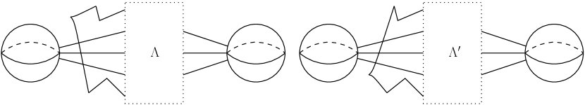
Figure 29. Front ($xz$) diagrams for Legendrian links $\Lambda,\Lambda^{\prime}$ in normal form related by Gompf move 6. The corners in these fronts are understood to be smoothed out.

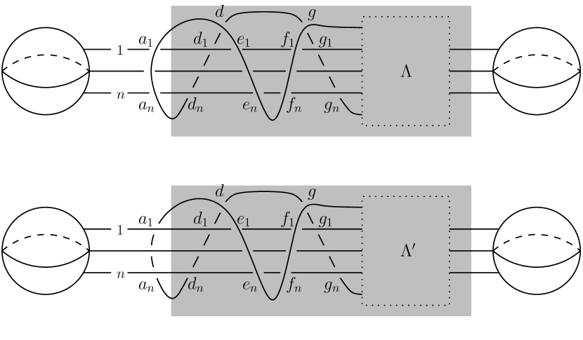
Figure 30. The $xy$ projections for $\Lambda$ and $\Lambda^{\prime}$ given in Figure 29, with some crossings labeled. The dotted boxes are identical (and correspond to the dotted boxes in Figure 29), as are the two shaded regions.

Let $\Lambda$ and $\Lambda^{\prime}$ be Legendrian links in $\#^{k}(S^{1}\times S^{2})$ related by Gompf move 6. Perturb the fronts of $\Lambda$ and $\Lambda^{\prime}$ to be in normal form, and then further perturb them to take the form shown in Figure 29. Then the corresponding $xy$ projections are in $xy$-normal form as shown in Figure 30.

By Proposition B.3, it suffices to show that the DGAs for $\Lambda$ and $\Lambda^{\prime}$ associated to the $xy$ projections shown in Figure 30 are stable tame isomorphic. Denote these DGAs by $(\mathcal{A},\partial)$ and $(\mathcal{A}^{\prime},\partial^{\prime})$ respectively. We will show that these DGAs are both stable tame isomorphic to a third DGA $(\mathcal{A}^{\prime\prime},\partial^{\prime\prime})$, which we now define.

Note that $\mathcal{A}$ is generated by internal generators $c_{ij}^{p}$, where $1\leq i,j\leq n$, $p\geq 0$, and $i<j$ if $p=0$, along with external generators corresponding to crossings in $\pi_{xy}(\Lambda)$, including $a_{1},\ldots,a_{n}$ as marked in Figure 30 as well as $b_{1},\ldots,b_{n}$ and so forth. Let $\mathcal{A}^{\prime\prime}$ be the algebra generated by the internal generators $c_{ij}^{p}$, along with all external generators except $a_{1},\ldots,a_{n}$. This algebra inherits a grading from $\mathcal{A}$. There is an algebra projection map $\pi:\thinspace\mathcal{A}\to\mathcal{A}^{\prime\prime}$ that maps $a_{1},\ldots,a_{n}$ to $0$ and every other generator of $\mathcal{A}$ to itself; that is, it projects away any word involving any $a_{i}$. We now define $\partial^{\prime\prime}:\thinspace\mathcal{A}^{\prime\prime}\to\mathcal{A}^{\prime\prime}$ by

$$\partial^{\prime\prime}=\pi\circ\partial.$$

We will prove that $(\mathcal{A},\partial)$ and $(\mathcal{A}^{\prime\prime},\partial^{\prime\prime})$ are stable tame isomorphic. The proof that $(\mathcal{A}^{\prime},\partial^{\prime})$ and $(\mathcal{A}^{\prime\prime},\partial^{\prime\prime})$ are stable tame isomorphic is entirely similar. (Note for this purpose that there is also a projection map $\pi^{\prime}:\thinspace\mathcal{A}^{\prime}\to\mathcal{A}^{\prime\prime}$ that sends the generators $a_{1},\ldots,a_{n}$ of $\mathcal{A}^{\prime}$ to $0$ and acts as the identity on all other generators, and that $\partial^{\prime\prime}=\pi^{\prime}\circ\partial^{\prime}$.)

For grading purposes, let $(m(1),\ldots,m(n))$ be the Maslov potentials associated to strands $1,\ldots,n$ passing through the handle, and let $m(0)$ be the Maslov potential associated to the strand in the front projection of $\Lambda$ in Figure 29 that crosses over the other strands (and includes the bottom half of the left cusp). Then we have

$$|a_{i}|=m(0)-m(i)$$

for $1\leq i\leq n$. Write $\sigma_{i}=(-1)^{m(i)}$ for $1\leq i\leq n$, and $\sigma=(-1)^{m(0)}$; then $\operatorname{sgn}(c_{ij}^{p})=-\sigma_{i}\sigma_{j}$ and $\operatorname{sgn}(a_{i})=\sigma\sigma_{i}$.

Let $\tilde{\mathcal{A}}$ be the algebra generated by the generators of $\mathcal{A}$, along with infinite families of generators

$$\{a_{q}\}_{q=n+1}^{\infty}\text{ and }\{b_{q}\}_{q=n+1}^{\infty}$$

with grading given by $|a_{q+n}|=|a_{q}|+2$ for all $q\geq 1$ and $|b_{q}|=|a_{q}|-1$ for all $q\geq n+1$. Extend $\partial$ from $\mathcal{A}$ to $\tilde{\mathcal{A}}$ by setting

$$\partial(a_{q})=b_{q},~{}~{}~{}~{}~{}~{}~{}\partial(b_{q})=0\text{ for }q\geq n+1.$$

Then $(\tilde{\mathcal{A}},\partial)$ is a stabilization of $(\mathcal{A},\partial)$.

We can also view $\tilde{\mathcal{A}}$ as being generated by the generators of $\mathcal{A}^{\prime\prime}$, along with $\{a_{q}\}_{q=1}^{\infty}$ and $\{b_{q}\}_{q=n+1}^{\infty}$. Extend $\partial^{\prime\prime}$ from $\mathcal{A}^{\prime\prime}$ to $\tilde{\mathcal{A}}$ by setting

$$\partial^{\prime\prime}(b_{q+n})=a_{q},~{}~{}~{}~{}~{}~{}\partial^{\prime\prime}(a_{q})=0\text{ for }q\geq 1;$$

note that this is a graded differential since $|b_{q+n}|=|a_{q}|+1$. Then $(\tilde{\mathcal{A}},\partial^{\prime\prime})$ is a stabilization of $(\mathcal{A}^{\prime\prime},\partial^{\prime\prime})$. It thus suffices to establish the following result.

Lemma B.12.

$(\tilde{\mathcal{A}},\partial)$ and $(\tilde{\mathcal{A}},\partial^{\prime\prime})$ are tamely isomorphic.

We will construct the tame isomorphism in Lemma B.12 in two steps, one of which is deferred to Section B.2.G. Let $\tilde{\mathcal{A}}_{0}$ denote the subalgebra of $\tilde{\mathcal{A}}$ generated by internal generators $c_{ij}^{p}$ along with $a_{i}$ for $i\geq 1$ and $b_{i}$ for $i\geq n+1$. This is in fact a differential subalgebra of $\tilde{\mathcal{A}}$ with respect to $\partial$: indeed, by inspection of Figure 30 and the definition of the internal differential, we have

$$\partial(a_{i}) =-\sum_{j=1}^{i-1}\sigma\sigma_{j}a_{j}c_{ji}^{0},\hskip 12.91663pt\text{ for }i\leq n,$$

$$\partial(c_{ij}^{p}) =\delta_{ij}\delta_{1p}+\sum_{\ell=0}^{p}\sum_{m=1}^{n}\sigma_{i}\sigma_{m}c_{im}^{\ell}c_{mj}^{p-\ell}.$$

In Section B.2.G, we will establish the following result.

Lemma B.13.

There is a tame automorphism $\Psi$ of $\tilde{\mathcal{A}}$ with the following properties:

1. $\Psi$ acts as the identity on all generators of $\mathcal{A}$ except for $\{a_{i}\}_{i\geq 1}$ and $\{b_{i}\}_{i\geq n+1}$, and restricts to a tame automorphism of $\tilde{\mathcal{A}}_{0}\subset\tilde{\mathcal{A}}$;

2. for $q\leq n$,

   $$\Psi(a_{q})=a_{q}-\sum_{m=n+1}^{q+n-1}\sigma\sigma_{m}b_{m}c_{m-n,q}^{0};$$

3. on $\tilde{\mathcal{A}}_{0}$,

   $$\Psi\circ\partial=\partial^{\prime\prime}\circ\Psi.$$

We now use Lemma B.13 to prove Lemma B.12 and thus invariance under Gompf move 6.

Proof of Lemma B.12.

Define $\Omega:\thinspace\tilde{\mathcal{A}}\to\tilde{\mathcal{A}}$ to be the algebra map given by

$$\Omega(e_{i}) =e_{i}+b_{i+n},\hskip 21.52771pt1\leq i\leq n,$$

$$\Omega(d) =d+\sum_{i=1}^{n}b_{n+i}d_{i},$$

and $\Omega(x)=x$ for all other generators of $\tilde{\mathcal{A}}$. Note that $\Omega$ is an elementary automorphism with respect to any ordering for which $b_{n+1},\ldots,b_{2n}$ are less than the $e_{i}$, $d_{i}$, and $d$. We will show that

(B.4) $$\Omega\circ\Psi\circ\partial(x)=\partial^{\prime\prime}\circ\Omega\circ\Psi(x)$$

for all generators $x$ of $\tilde{\mathcal{A}}$, and thus $\Omega\circ\Psi$ is the desired tame automorphism of $\tilde{\mathcal{A}}$ intertwining $\partial$ and $\partial^{\prime\prime}$.

For a generator $x$ of $\tilde{\mathcal{A}}_{0}\subset\tilde{\mathcal{A}}$, since $\Omega$ restricts to the identity on $\tilde{\mathcal{A}}_{0}$, we have $\Omega\Psi\partial(x)=\Psi\partial(x)=\partial^{\prime\prime}\Psi(x)=\partial^{\prime\prime}\Omega\Psi(x)$ by Lemma B.13(3). Otherwise, $x$ corresponds to a crossing in the shaded region of the top diagram in Figure 30. An inspection of Figure 30 shows that unless $x=d$ or $x=e_{i}$ for some $1\leq i\leq n$, $\partial(x)$ does not involve any of $a_{1},\ldots,a_{n},e_{1},\ldots,e_{n}$; then by Lemma B.13(1), $\partial(x)=\Psi\partial(x)$, and so $\Omega\Psi\partial(x)=\Omega\partial(x)=\partial(x)=\partial^{\prime\prime}(x)=\partial^{\prime\prime}\Omega\Psi(x)$.

It remains to check (B.4) for $x=d$ or $x=e_{i}$. To this end, another inspection of Figure 30 yields

$$\partial(d_{i}) =-g_{i}+\sum_{j=i+1}^{n}c_{ij}^{0}d_{j}, 1\leq i\leq n,$$

$$\partial(e_{i}) =a_{i}-f_{i}+\sum_{j<i}\sigma\sigma_{j}e_{j}c_{ji}^{0}, 1\leq i\leq n,$$

$$\partial(d) =1-g+\sum_{i=1}^{n}a_{i}d_{i}-\sum_{i=1}^{n}\sigma\sigma_{i}e_{i}g_{i}.$$

Then by direct calculation and Lemma B.13(2), we have

$$\Omega\Psi\partial(e_{i}) =\Omega\left(a_{i}-f_{i}+\sum_{j=1}^{i-1}\sigma\sigma_{j}(e_{j}-b_{j+n})c_{ji}^{0}\right)$$

$$=a_{i}-f_{i}+\sum_{j<i}\sigma\sigma_{j}e_{j}c_{ji}^{0}$$

$$=\partial^{\prime\prime}(e_{i}+b_{n+i})$$

$$=\partial^{\prime\prime}\Omega\Psi(e_{i})$$

and

$$\Omega\Psi\partial(d) =1-g+\sum_{i=1}^{n}\left((a_{i}-\sum_{j=1}^{i-1}\sigma\sigma_{j}b_{j+n}c_{ji}^{0})d_{i}-\sigma\sigma_{i}(e_{i}+b_{i+n})g_{i}\right)$$

$$=\partial^{\prime\prime}(d)+\sum_{i}(a_{i}d_{i}-\sigma\sigma_{i}b_{i+n}g_{i})-\sum_{1\leq j<i\leq n}\sigma\sigma_{j}b_{n+j}c_{ji}^{0}d_{i}$$

$$=\partial^{\prime\prime}(d+\sum_{i=1}^{n}b_{i+n}d_{i})$$

$$=\partial^{\prime\prime}\Omega\Psi(d).\qed$$

B.2.G. Invariance under Gompf move 6, part 2

In this section we prove Lemma B.13, completing the proof of invariance for Gompf move 6. When defining the tame isomorphism $\Psi$, it will be convenient to replace the notation $c_{ij}^{p}$ by $c_{ab}$ for $a,b\in\mathbb{Z}$, where $c_{ab}$ is defined as follows: write $a=a_{1}n+a_{2}$ and $b=b_{1}n+b_{2}$ for $1\leq a_{2},b_{2}\leq n$; then

$$c_{ab}=\begin{cases}0&a\leq b\\ c_{a_{2},b_{2}}^{b_{1}-a_{1}}&a>b.\end{cases}$$

Also extend $\sigma_{1},\ldots,\sigma_{n}$ to $\sigma_{a}$ for all $a\in\mathbb{Z}$ by setting $\sigma_{a}=\sigma_{a_{2}}$. With this notation, the following result is trivial to check.

Lemma B.14.

1. For any $a,b\in\mathbb{Z}$, $c_{ab}=c_{a+n,b+n}$.

2. For any $a,b\in\mathbb{Z}$, $\partial(c_{ab})=\delta_{a+n,b}+\sum_{m=a+1}^{b-1}\sigma_{a}\sigma_{m}c_{am}c_{mb}$.

For $s\geq n$, define a map $\partial_{s}:\thinspace\tilde{\mathcal{A}}_{0}\to\tilde{\mathcal{A}}_{0}$ as follows:

$$\partial_{s}(a_{q}) =\begin{cases}b_{q},&q>s,\\ -\displaystyle{\sum_{m=s-n+1}^{q-1}\sigma\sigma_{m}a_{m}c_{mq}},&q\leq s,\\ 0,&q\leq s-n+1,\end{cases}$$

$$\partial_{s}(b_{q}) =\begin{cases}0,&q>s\\ a_{q-n},&(n+1\leq\,)\,q\leq s,\end{cases}$$

$$\partial_{s}(c_{ab}) =\partial(c_{ab}).$$

(The case $q\leq s-n+1$ in the definition of $\partial_{s}(a_{q})$ is superfluous, following from the expression for $q\leq s$, but is included for ease of reference.) Extend $\partial_{s}$ to all of $\tilde{\mathcal{A}}_{0}$ by the Leibniz rule. Note that $\partial_{n}=\partial$.

We next claim that $\partial_{n},\partial_{n+1},\ldots$ are related by tame automorphisms of $\tilde{\mathcal{A}}_{0}$. To this end, for $s\geq n+1$, define algebra maps $\phi_{s},\psi_{s}:\thinspace\tilde{\mathcal{A}}_{0}\to\tilde{\mathcal{A}}_{0}$ as follows:

$$\phi_{s}(b_{s}) =b_{s}-\sum_{m=s-n}^{s-1}\sigma\sigma_{m}a_{m}c_{ms},$$

$$\psi_{s}(a_{q}) =a_{q}-\sigma\sigma_{s}b_{s}c_{s,q+n}, \text{for }(s-n+1\leq\,)\,q\leq s,$$

and $\phi_{s},\psi_{s}$ act as the identity on all generators of $\tilde{\mathcal{A}}_{0}$ besides $b_{s}$ for $\phi_{s}$ and $a_{s-n+1},\ldots,a_{s}$ for $\psi_{s}$.

Lemma B.15.

For all $s\geq n+1$, we have $\psi_{s}\phi_{s}\partial_{s-1}=\partial_{s}\psi_{s}\phi_{s}$.

Proof.

We will show that $\psi_{s}\phi_{s}\partial_{s-1}(x)=\partial_{s}\psi_{s}\phi_{s}(x)$ for all generators $x$ of $\tilde{\mathcal{A}}_{0}$. Since $\psi_{s},\phi_{s}$ do not affect generators of the form $c_{ij}^{p}$, $\psi_{s}\phi_{s}\partial_{s-1}(c_{ij}^{p})=\partial(c_{ij}^{p})=\partial_{s}\psi_{s}\phi_{s}(c_{ij}^{p})$. Similarly, it follows from the definitions of $\partial_{s},\partial_{s-1},\psi_{s},\phi_{s}$ that if $q>s$, we have $\psi_{s}\phi_{s}\partial_{s-1}(a_{q})=b_{q}=\partial_{s}\psi_{s}\phi_{s}(a_{q})$ and $\psi_{s}\phi_{s}\partial_{s-1}(b_{q})=0=\partial_{s}\psi_{s}\phi_{s}(a_{q})$; and if $q<s$, we have $\psi_{s}\phi_{s}\partial_{s-1}(b_{q})=a_{q-n}=\partial_{s}\psi_{s}\phi_{s}(b_{q})$.

It remains to check $x=a_{q}$ for $q\leq s$ and $x=b_{s}$. For $x=a_{q}$ with $q<s$, we have

$$\psi_{s}\phi_{s}\partial_{s-1}(a_{q}) =\psi_{s}\phi_{s}\left(-\sum_{m=s-n}^{q-1}\sigma\sigma_{m}a_{m}c_{mq}\right)$$

$$=-\sum_{m=s-n}^{q-1}\sigma\sigma_{m}(a_{m}-\sigma\sigma_{s}b_{s}c_{s,m+n})c_{mq}$$

$$=-\left(\sum_{m=s-n+1}^{q-1}\sigma\sigma_{m}a_{m}c_{mq}\right)-\sigma\sigma_{s}a_{s-n}c_{s,q+n}+b_{s}\partial(c_{s,q+n})$$

$$=\partial_{s}(a_{q}-\sigma\sigma_{s}b_{s}c_{s,q+n})$$

$$=\partial_{s}\psi_{s}\phi_{s}(a_{q}),$$

while for $x=a_{s}$, we have

$$\psi_{s}\phi_{s}\partial_{s-1}(a_{s}) =\psi_{s}\left(b_{s}-\sum_{m=s-n}^{s-1}\sigma\sigma_{m}a_{m}c_{ms}\right)$$

$$=b_{s}-\sum_{m=s-n}^{s-1}\sigma\sigma_{m}a_{m}c_{ms}+\sum_{m=s-n}^{s-1}\sigma_{m}\sigma_{s}b_{s}c_{s,m+n}c_{m+n,s+n}$$

$$=b_{s}+(\partial_{s}(a_{s})-\sigma\sigma_{s-n}a_{s-n}c_{s-n,s})+b_{s}(\partial(c_{s,s+n})-1)$$

$$=\partial_{s}(a_{s}-\sigma\sigma_{s}b_{s}c_{s,s+n})$$

$$=\partial_{s}\psi_{s}\phi_{s}(a_{s}).$$

Finally, for $x=b_{s}$, we have

$$\partial_{s}\psi_{s}\phi_{s}(b_{s}) =\partial_{s}(b_{s})-\partial_{s}\psi_{s}\phi_{s}\left(\sum_{m=s-n}^{s-1}\sigma\sigma_{m}a_{m}c_{ms}\right)$$

$$=a_{s-n}-\psi_{s}\phi_{s}\partial_{s-1}\left(\sum_{m=s-n}^{s-1}\sigma\sigma_{m}a_{m}c_{ms}\right)$$

$$=a_{s-n}-\psi_{s}\phi_{s}(a_{s-n})$$

$$=0$$

$$=\psi_{s}\phi_{s}\partial_{s-1}(b_{s}),$$

where the second equality follows from $\psi_{s}\phi_{s}\partial_{s-1}(x)=\partial_{s}\psi_{s}\phi_{s}(x)$ for $x=a_{m}$ and $x=c_{ms}$, and the third equality is a direct computation:

$$\partial_{s-1} \left(\sum_{m=s-n}^{s-1}\sigma\sigma_{m}a_{m}c_{ms}\right)$$

$$=\sum_{m=s-n}^{s-1}\left(-\sum_{\ell=s-n}^{m-1}\sigma_{m}\sigma_{\ell}a_{\ell}c_{\ell m}c_{ms}+a_{m}\left(\sum_{\ell=m+1}^{s-1}\sigma_{m}\sigma_{\ell}c_{m\ell}c_{\ell s}+\delta_{m+n,s}\right)\right)$$

$$=a_{s-n}-\sum_{s-n\leq\ell<m\leq s-1}\sigma_{m}\sigma_{\ell}a_{\ell}c_{\ell m}c_{ms}+\sum_{s-n\leq m<\ell\leq s-1}\sigma_{m}\sigma_{\ell}a_{m}c_{m\ell}c_{\ell s}$$

$$=a_{s-n}.$$

This completes the verification of the lemma for all generators of $\tilde{\mathcal{A}}_{0}$. ∎

For $s\geq n+1$, define $\Phi_{s}:\thinspace\tilde{\mathcal{A}}_{0}\to\tilde{\mathcal{A}}_{0}$ by

$$\Phi_{s}=\psi_{s}\circ\phi_{s}\circ\psi_{s-1}\circ\phi_{s-1}\circ\cdots\circ\psi_{n+1}\circ\phi_{n+1}.$$

By Lemma B.15, we have $\Phi_{s}\circ\partial_{n}\circ\Phi_{s}^{-1}=\partial_{s}$ on $\tilde{\mathcal{A}}_{0}$.

Now define $\partial_{\infty}:\thinspace\tilde{\mathcal{A}}_{0}\to\tilde{\mathcal{A}}_{0}$ by

$$\partial_{\infty}(c_{ij}^{p}) =\partial(c_{ij}^{p})$$

$$\partial_{\infty}(a_{q}) =0 q\geq 1$$

$$\partial_{\infty}(b_{q}) =a_{q-n} q\geq n+1.$$

Intuitively, this is the limit of $\partial_{s}$ as $s\to\infty$. Note that on $\tilde{\mathcal{A}}_{0}\subset\tilde{\mathcal{A}}$, $\partial_{\infty}$ agrees with $\partial^{\prime\prime}$. If we can construct the “limit” automorphism $\Phi=\lim_{s\to\infty}\Phi_{s}$, then we should have $\Phi\circ\partial_{n}\circ\Phi^{-1}=\partial_{\infty}$ on $\tilde{\mathcal{A}}_{0}$, and $\Phi$ intertwines $\partial=\partial_{n}$ and $\partial^{\prime\prime}=\partial_{\infty}$ on $\tilde{\mathcal{A}}_{0}$.

To make this rigorous, consider the following algebra maps $\Psi_{1},\Psi_{2}:\thinspace\tilde{\mathcal{A}}_{0}\to\tilde{\mathcal{A}}_{0}$: $\Psi_{1}$ is the identity on all generators except for the $a_{q}$, and

$$\Psi_{1}(a_{q})=a_{q}-\sum_{m=\max(q,n+1)}^{q+n-1}\sigma\sigma_{m}b_{m}c_{m,q+n}$$

for $q\geq 1$; $\Psi_{2}$ is the identity on all generators except for the $b_{q}$, and

$$\Psi_{2}(b_{q})=b_{q}-\sum_{m=q-n}^{q-1}\sigma\sigma_{m}(\psi_{n+1}^{-1}\psi_{n+2}^{-1}\cdots\psi_{q-1}^{-1}(a_{m}))c_{mq}$$

for $q\geq n+1$. Then $\Psi_{1}$ is an elementary automorphism with respect to any ordering of $\tilde{\mathcal{A}}_{0}$ for which

$$c_{ij}^{0},c_{ij}^{1}<a_{1}<b_{n+1}<a_{2}<b_{n+2}<a_{3}<b_{n+3}<\cdots$$

where $c_{ij}^{0},c_{ij}^{1}$ are ordered before all $a_{q}$ and $b_{q}$ for all $1\leq i,j\leq n$, and $\Psi_{2}$ is an elementary automorphism with respect to any ordering for which

$$c_{ij}^{0},c_{ij}^{1}<a_{1}<\cdots<a_{n}<b_{n+1}<a_{n+1}<b_{n+2}<\cdots.$$

(To verify this second statement, note that $\psi_{s}^{-1}(a_{m})=a_{m}+\sigma\sigma_{s}b_{s}c_{s,m+n}$ for $m\leq s$, and so when $m\leq q-1$, $\psi_{n+1}^{-1}\cdots\psi_{q-1}^{-1}(a_{m})$ can only involve $a_{m}$, $b_{s}$ with $s\leq q-1$, and $c_{s,m+n}$ with $s\geq n+1$.)

We now define the map $\Psi:\thinspace\tilde{\mathcal{A}}_{0}\to\tilde{\mathcal{A}}_{0}$ by $\Psi=\Psi_{1}\circ\Psi_{2}$. By the above discussion, $\Psi$ is a tame automorphism of $\tilde{\mathcal{A}}_{0}$.

Lemma B.16.

1. $\partial_{s}(a_{q})=\partial_{\infty}(a_{q})$ for $s\geq q+n-1$, and $\partial_{s}(b_{q})=\partial_{\infty}(b_{q})$ for $s\geq q$.

2. $\Phi_{s}(a_{q})=\Psi(a_{q})$ for $s\geq q+n-1$, and $\Phi_{s}(b_{q})=\Psi(b_{q})$ for $s\geq q+n-2$.

Proof.

(1) is clear from the definition of $\partial_{s}$ and $\partial_{\infty}$.

To establish (2), rewrite $\Phi_{s}$ for $s\geq n+1$ as follows:

(B.5) $$\Phi_{s}=\psi_{s}\circ\psi_{s-1}\circ\cdots\circ\psi_{n+1}\circ\tilde{\phi}_{s}\circ\tilde{\phi}_{s-1}\circ\cdots\circ\tilde{\phi}_{n+1},$$

where $\tilde{\phi}_{q}=(\psi_{q-1}\cdots\psi_{n+1})^{-1}\circ\phi_{q}\circ(\psi_{q-1}\cdots\psi_{n+1})$ for $q\geq n+1$. Since $\phi_{q}$ acts as the identity on all generators but $b_{q}$, and the definitions of $\psi_{q-1},\ldots,\psi_{n+1}$ do not involve $b_{q}$, we conclude that $\tilde{\phi}_{q}$ acts as the identity on all generators of $\tilde{\mathcal{A}}_{0}$ except $b_{q}$, and

$$\tilde{\phi}_{q}(b_{q}) =\psi_{n+1}^{-1}\cdots\psi_{q-1}^{-1}(\phi_{q}(b_{q}))=b_{q}-\sum_{m=q-n}^{q-1}\sigma\sigma_{m}(\psi_{n+1}^{-1}\cdots\psi_{q-1}^{-1})(a_{m})c_{mq}$$

$$=\Psi_{2}(b_{q}).$$

Note that by the discussion preceding the lemma, $\Psi_{2}(b_{q})$ involves only $a_{\ell}$ with $\ell<q$, along with $b$’s and $c$’s.

From (B.5), we have $\Phi_{s}(a_{q})=(\psi_{s}\cdots\psi_{n+1})(a_{q})$. Using the definitions of $\Phi_{s}$, $\phi_{s}$, and $\psi_{s}$, one can easily check by induction on $s\geq n+1$ that

$$\Phi_{s}(a_{q}) =(\psi_{s}\cdots\psi_{n+1})(a_{q})$$

$$=\begin{cases}a_{q},&s<q\\ a_{q}-\sum_{m=\max(q,n+1)}^{s}\sigma\sigma_{m}b_{m}c_{m,q+n},&q\leq s\leq q+n-2,\\ a_{q}-\sum_{m=\max(q,n+1)}^{q+n-1}\sigma\sigma_{m}b_{m}c_{m,q+n},&s\geq q+n-1,\end{cases}$$

and it follows that $\Phi_{s}(a_{q})=\Psi_{1}(a_{q})=\Psi(a_{q})$ when $s\geq q+n-1$.

Finally, let $s\geq q+n-2$. We have just shown that $(\psi_{s}\cdots\psi_{n+1})(x)=\Psi_{1}(x)$ if $x=a_{\ell}$ with $\ell<q$, and the same equation holds trivially if $x$ is a $b$ or $c$ generator. It follows that

$$\Phi_{s}(b_{q}) =(\psi_{s}\cdots\psi_{n+1})(\tilde{\phi}_{q}(b_{q}))=(\psi_{s}\cdots\psi_{n+1})(\Psi_{2}(b_{q}))=\Psi_{1}(\Psi_{2}(b_{q}))$$

$$=\Psi(b_{q}),$$

and this completes the proof of (2). ∎

We are now in position to prove Lemma B.13.

Proof of Lemma B.13.

The tame automorphism $\Psi$ of $\tilde{\mathcal{A}}_{0}$ is the one defined in the above discussion. Properties (1) and (2) in the statement of Lemma B.13 are direct consequences of the construction of $\Psi$. It remains to establish property (3), which we can do by checking that $\Psi\partial(x)=\partial^{\prime\prime}\Psi(x)$ for all generators $x$ of $\tilde{\mathcal{A}}_{0}$.

If $x=c_{ij}^{p}$, then $\Psi\partial(c_{ij}^{p})=\partial(c_{ij}^{p})=\partial^{\prime\prime}(c_{ij}^{p})=\partial^{\prime\prime}\Psi(c_{ij}^{p})$. If $x=a_{q}$ with $q\geq 1$, then choose any $s\geq q+n-1$. By Lemma B.16(2), we have $\Phi_{s}(a_{q})=\Psi(a_{q})$; since $\partial_{n}(a_{q})$ involves only $a_{1},\ldots,a_{q-1}$ and $c$, we also have $\Psi\partial_{n}(a_{q})=\Phi_{s}\partial_{n}(a_{q})$. Furthermore, $\Psi(a_{q})=\Psi_{1}(a_{q})$ involves only $a_{\ell}$ with $\ell\leq q$, $b_{\ell}$ with $\ell\leq n+q-1$, and $c$, and so by Lemma B.16(1) we have $\partial_{\infty}(\Psi(a_{q}))=\partial_{s}(\Psi(a_{q}))$. Thus

$$\Psi\partial(a_{q}) =\Psi\partial_{n}(a_{q})=\Phi_{s}\partial_{n}(a_{q})=\partial_{s}\Phi_{s}(a_{q})=\partial_{s}\Psi(a_{q})$$

$$=\partial_{\infty}\Psi(a_{q})=\partial^{\prime\prime}\Psi(a_{q}).$$

Finally, consider the case $x=b_{q}$ with $q\geq n+1$, and choose any $s\geq q+n-2$. From the discussion preceding Lemma B.16, $\Psi_{2}(b_{q})$ involves only $c$, $a_{\ell}$ with $\ell\leq q-1$, and $b_{\ell}$ with $\ell\leq q$; then $\Psi(b_{q})=\Psi_{1}(\Psi_{2}(b_{q}))$ involves only $c$, $a_{\ell}$ with $\ell\leq q-1$, and $b_{\ell}$ with $\ell\leq n+q-2$. By Lemma B.16(1), it follows that $\partial_{s}\Psi(b_{q})=\partial_{\infty}\Psi(b_{q})$. Also, by Lemma B.16(2), $\Phi_{s}(b_{q})=\Psi(b_{q})$. Thus

$$\Psi\partial(b_{q})=0=\Phi_{s}\partial_{n}(b_{q})=\partial_{s}\Phi_{s}(b_{q})=\partial_{s}\Psi(b_{q})=\partial_{\infty}\Psi(b_{q})=\partial^{\prime\prime}\Psi(b_{q})$$

and the proof is complete. ∎

B.2.H. Proof of Theorem 2.18

Consider two front diagrams that represent Legendrian-isotopic links in normal form in $\#^{k}(S^{1}\times S^{2})$. By [19], these diagrams are related by a sequence of the basic moves mentioned above. (Since our definition of the DGA requires a choice of base point on each component of the link, we should also include moves that fix the fronts but move base points along the components. However, such moves simply change the differential by conjugation by a particular tame automorphism of the algebra, replacing each generator by itself times some product of powers of $t_{i}$. See [27, section 2.5].)

By Proposition B.3, two Legendrian links in normal form that are related by Legendrian isotopy inside the box $[0,A]\times[-M,M]$ have DGAs that are stable tame isomorphic. Propositions B.5, B.9, and B.11 show invariance under Gompf moves 4, 5, and 6. Invariance for the alternate ($180^{\circ}$ rotated) versions of Gompf moves 4 and 6 follows from invariance under the usual versions, along with Lemma B.2 and the fact that two semifree DGAs $(\mathcal{A},\partial),(\mathcal{A}^{\prime},\partial^{\prime})$ are stable tame isomorphic if and only if $(\mathcal{A},\partial_{\textrm{op}}),(\mathcal{A}^{\prime},\partial^{\prime}_{\textrm{op}})$ are stable tame isomorphic. ∎

References

- [1] Alberto Abbondandolo, Alessandro Portaluri, and Matthias Schwarz. The homology of path spaces and Floer homology with conormal boundary conditions. J. Fixed Point Theory Appl., 4(2):263–293, 2008. arXiv:0810.1977.
- [2] Mohammed Abouzaid. A cotangent fibre generates the Fukaya category. Adv. Math., 228(2):894–939, 2011. arXiv:1003.4449.
- [3] Mohammed Abouzaid and Paul Seidel. Altering symplectic manifolds by homologous recombination. arXiv:1007.3281.
- [4] F. Bourgeois, Y. Eliashberg, H. Hofer, K. Wysocki, and E. Zehnder. Compactness results in symplectic field theory. Geom. Topol., 7:799–888, 2003. arXiv:math/0308183.
- [5] Frédéric Bourgeois, Tobias Ekholm, and Yasha Eliashberg. Effect of Legendrian surgery. Geom. Topol., 16(1):301–389, 2012. With an appendix by Sheel Ganatra and Maksim Maydanskiy. arXiv:0911.0026.
- [6] Frédéric Bourgeois and Otto van Koert. Action filtration and contact homology of connected sums. Work in progress.
- [7] Yuri Chekanov. Differential algebra of Legendrian links. Invent. Math., 150(3):441–483, 2002.
- [8] Kai Cieliebak. Handle attaching in symplectic homology and the chord conjecture. J. Eur. Math. Soc. (JEMS), 4(2):115–142, 2002.
- [9] Kai Cieliebak and Yakov Eliashberg. From Stein to Weinstein and back, volume 59 of American Mathematical Society Colloquium Publications. American Mathematical Society, Providence, RI, 2012.
- [10] Tobias Ekholm. Morse flow trees and Legendrian contact homology in 1-jet spaces. Geom. Topol., 11:1083–1224, 2007. arXiv:math/0509386.
- [11] Tobias Ekholm. Rational symplectic field theory over for exact Lagrangian cobordisms. J. Eur. Math. Soc. (JEMS), 10(3):641–704, 2008. arXiv:math/0612029.
- [12] Tobias Ekholm, John Etnyre, and Michael Sullivan. Orientations in Legendrian contact homology and exact Lagrangian immersions. Internat. J. Math., 16(5):453–532, 2005. arXiv:math/0408411.
- [13] Tobias Ekholm, John Etnyre, and Michael Sullivan. Legendrian contact homology in . Trans. Amer. Math. Soc., 359(7):3301–3335 (electronic), 2007. arXiv:math/0505451.
- [14] Tobias Ekholm, John B Etnyre, Lenhard Ng, and Michael G Sullivan. Knot contact homology. Geom. Topol., 17(2):975–1112, 2013. arXiv:1109.1542.
- [15] Tobias Ekholm, Ko Honda, and Tamas Kálmán. Legendrian knots and exact Lagrangian cobordisms. arXiv:1212.1519.
- [16] Yakov Eliashberg and Maia Fraser. Classification of topologically trivial Legendrian knots. In Geometry, topology, and dynamics (Montreal, PQ, 1995), volume 15 of CRM Proc. Lecture Notes, pages 17–51. Amer. Math. Soc., Providence, RI, 1998.
- [17] John B. Etnyre, Lenhard L. Ng, and Joshua M. Sabloff. Invariants of Legendrian knots and coherent orientations. J. Symplectic Geom., 1(2):321–367, 2002. arXiv:math/0101145.
- [18] Kenji Fukaya, Yong-Geun Oh, Hiroshi Ohta, and Kaoru Ono. Lagrangian intersection Floer theory: anomaly and obstruction. Parts I and II, volume 46 of AMS/IP Studies in Advanced Mathematics. American Mathematical Society, Providence, RI, 2009.
- [19] Robert E. Gompf. Handlebody construction of Stein surfaces. Ann. of Math. (2), 148(2):619–693, 1998.
- [20] Helmut Hofer, Kris Wysocki, and Eduard Zehnder. A general Fredholm theory. III. Fredholm functors and polyfolds. Geom. Topol., 13(4):2279–2387, 2009. arXiv:0810.0736.
- [21] Michael Hutchings. Quantitative embedded contact homology. J. Differential Geom., 88(2):231–266, 2011. arXiv:1005.2260.
- [22] Mark McLean. Lefschetz fibrations and symplectic homology. Geom. Topol., 13(4):1877–1944, 2009. arXiv:0709.1639.
- [23] Emmy Murphy. Loose Legendrian embeddings in high dimensional contact manifolds. arXiv:1201.2245.
- [24] Lenhard Ng. Combinatorial knot contact homology and transverse knots. Adv. Math., 227(6):2189–2219, 2011. arXiv:1010.0451.
- [25] Lenhard Ng. A topological introduction to knot contact homology. In Contact and Symplectic Topology, volume 26 of Bolyai Soc. Math. Stud., pages 485–530. Springer, Berlin, 2014. arXiv:1210.4803.
- [26] Lenhard Ng and Daniel Rutherford. Satellites of Legendrian knots and representations of the Chekanov-Eliashberg algebra. Algebr. Geom. Topol., 13(5):3047–3097, 2013. arXiv:1206.2259.
- [27] Lenhard L. Ng. Computable Legendrian invariants. Topology, 42(1):55–82, 2003. arXiv:math/0011265.
- [28] Alexandru Oancea. The Künneth formula in Floer homology for manifolds with restricted contact type boundary. Math. Ann., 334(1):65–89, 2006. arXiv:math/0403376.
- [29] Joshua M. Sabloff. Invariants of Legendrian knots in circle bundles. Commun. Contemp. Math., 5(4):569–627, 2003. arXiv:math/0208214.
- [30] Joshua M. Sabloff. Augmentations and rulings of Legendrian knots. Int. Math. Res. Not., (19):1157–1180, 2005. arXiv:math/0409032.
- [31] Clayton Shonkwiler and David Shea Vela-Vick. Legendrian contact homology and nondestabilizability. J. Symplectic Geom., 9(1):33–44, 2011. arXiv:0910.3914.