NLO QCD corrections to Higgs boson production in association
with a top quark pair and a jet

Abstract

We present the calculation of the cross section for Higgs boson production in association with a top quark pair plus one jet, at next-to-leading-order (NLO) accuracy in QCD. All mass dependence is retained without recurring to any approximation. After including the complete NLO QCD corrections, we observe a strong reduction in the scale dependence of the result. We also show distributions for the invariant mass of the top quark pair, with and without the additional jet, and for the transverse momentum and the pseudorapidity of the Higgs boson. Results for the virtual contributions are obtained with a novel reduction approach based on integrand decomposition via Laurent expansion, as implemented in the library Ninja. Cross sections and differential distributions are obtained with an automated setup which combines the GoSam and Sherpa frameworks.

I Introduction

The evidence of the existence of a new particle of mass between 125 and 126 GeV, initially reported about one year ago by the ATLAS and CMS collaborations Aad et al. (2012); Chatrchyan et al. (2012), has been confirmed with very high confidence level by more recent analyses, thus providing more stringent arguments in favor of the validity of the electroweak symmetry breaking mechanism. It is interesting to observe that all the analyses performed so far are in good agreement with the hypothesis that the new particle is the Higgs boson predicted by the Standard Model (SM). Indeed, rates and distributions are compatible with the assumption that the new particle is a scalar that couples to other SM particles with a strength proportional to their mass CMS-PAS-HIG-13- (005); Aad et al. (2013); Aaltonen et al. (2013). Accurate predictions are necessary and will play a crucial role for the complete determination of the nature of the Higgs boson Heinemeyer et al. (2013), in particular to shed light on the structure of its couplings to the other particles.

The production rate for a Higgs boson associated with a top-antitop pair ($t\bar{t}H$) is particularly interesting in this context, since it is directly proportional to the SM Yukawa coupling of the Higgs boson to the top quark. The study of differential observables and distributions will bring information on the coupling structure and on the parity of the Higgs particle Frederix et al. (2011); Degrande et al. (2012).

The difficulties related to the analysis of the $t\bar{t}H$ channel are well known. The combined production of three heavy particles requires a large center-of-mass energy for the initial partons, which is strongly suppressed by parton distribution functions. Furthermore, additional difficulties are represented by the presence of various challenging backgrounds and by the complexity of the final state, which make its kinematic reconstruction far from straightforward Artoisenet et al. (2013).

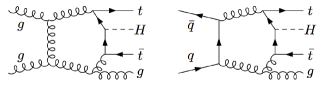
Figure 1: Sample of one-loop diagrams contributing to the NLO corrections to $gg\to t{\bar{t}}Hg$ and $q{\bar{q}}\to t{\bar{t}}Hg$.

At the parton level, the $t\bar{t}H$ production at next-to-leading order (NLO) in QCD has been known for some time Beenakker et al. (2001, 2003); Dawson et al. (2003a, b); Dittmaier et al. (2004). More recently, this process has been employed in a number of studies, motivated by the new analyses performed at the LHC Plehn et al. (2010); Frederix et al. (2011); Degrande et al. (2012); Artoisenet et al. (2013).

In this letter, we present the complete NLO QCD corrections to the process $pp\to t\bar{t}H+1$ jet ($t\bar{t}Hj$) at the LHC. Examples of contributing one-loop diagrams are depicted in Fig. 1. We illustrate the outcome of our calculation by showing the total cross section, and a selection of differential distributions.

The goal of the considered calculation is twofold. On the one hand, it is important for the phenomenological analyses at the LHC, in particular for the high-$p_{T}$ region, where the presence of the additional jet can be sensibly relevant. On the other hand, $t\bar{t}Hj$ constitutes the first application of a novel reduction algorithm for the evaluation of one-loop amplitudes, which strengthens the performances of the integrand decomposition Mastrolia et al. (2012), in particular in the presence of massive particles.

II Computational set-up

In perturbation theory, computations at the NLO accuracy require, aside from the evaluation of leading-order (LO) contributions, the calculation of both virtual and real-emission corrections. The Born and the real emission matrix elements are computed using Sherpa Gleisberg et al. (2009) and the library Amegic Krauss et al. (2002), which implements the Catani-Seymour dipole formalism Catani et al. (2002); Gleisberg and Krauss (2008). Sherpa also performs the integration over the phase space and the analysis. The virtual corrections are generated with the GoSam package Cullen et al. (2012), which combines automated diagram generation and algebraic manipulation Nogueira (1993); Vermaseren (2000); Reiter (2010); Cullen et al. (2011a); Kuipers et al. (2013) with $d$-dimensional integrand-level reduction techniques Ossola et al. (2007a, b); Ellis et al. (2008); Ossola et al. (2008); Mastrolia et al. (2008, 2010); Heinrich et al. (2010). The master integrals (MIs) are computed using OneLoop van Hameren (2011). The code generated by GoSam is linked to Sherpa by means of the Binoth Les Houches Accord (BLHA) Binoth et al. (2010) interface, which uses a system of order and contract files and allows for a direct communication between the two codes at running time. The same setup has been recently employed for the computation of NLO QCD corrections to $pp\to Hjj$ van Deurzen et al. (2013) and $pp\to Hjjj$ Cullen et al. (2013) (for the latter, in combination with MadDipole/MadEvent Maltoni and Stelzer (2003); Frederix et al. (2008, 2010)) and also for the analysis of the $t\bar{t}$ forward-backward asymmetry Hoeche et al. (2013).

For $t\bar{t}Hj$ production, the basic partonic processes identified by the Sherpa-GoSam contract file are:

$$q\,\bar{q}\,\to\,t\,\bar{t}\,H\,g\,,\qquad g\,g\,\to\,t\,\bar{t}\,H\,g\,,$$ (1)

while the remaining subprocesses can be obtained by proper crossings. The ultraviolet, the infrared, and the collinear singularities are regularized using dimensional reduction. The renormalization conditions are fixed along the lines of Beenakker et al. (2003); Dawson et al. (2003b), where the top mass is renormalized on-shell, while the strong coupling is renormalized in the $\overline{\mbox{MS}}$ scheme, decoupling the top quark from the running. In the case of LO [NLO] contributions, we describe the running of the strong coupling constant with one-loop [two-loop] accuracy. The wave functions of the gluon and of the quarks are renormalized on-shell, i.e. the corresponding renormalization constants cancel the external self-energy corrections exactly.

The virtual amplitudes of $t{\bar{t}}Hj$ have been decomposed in terms of MIs using for the first time the integrand reduction via Laurent expansion Mastrolia et al. (2012), implemented in the C++ library Ninja. This new algorithm exploits the complete knowledge of the analytic expression of the integrand and of the residues at the multiple cut to ameliorate the determination of the coefficients of the MIs with respect to the canonical integrand reduction Ossola et al. (2007a). Elaborating on the techniques introduced in Forde (2007); Kilgore (2007); Badger (2009), the series expansion combined with the integrand decomposition lowers the computational load and improves the accuracy of the results. Within this new algorithm, the sampling of the numerators and the subtractions of the higher-point residues, characterizing the triangular system-solving approach of the original integrand-reduction procedure, are avoided. Instead, the series expansion allows for a diagonal system-solving strategy, where the polynomial subtractions of the residues, when needed, are replaced by universal correction terms which have to be added to the coefficients of the Laurent series. These universal corrections, required only for the determination of the coefficients of 2-point and 1-point MIs, are obtained, once and for all, from the expansions of the generic polynomial forms of the residues at the triple and double cuts.

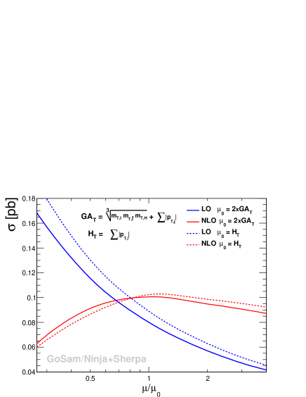
Figure 2: Scale dependence of the total cross section at LO and NLO.

The Ninja library, which has been interfaced to GoSam, implements the integrand reduction via Laurent expansion using a semi-analytic algorithm. The coefficients of the Laurent expansion of a generic integrand are efficiently computed by performing a polynomial division between the numerator and the set of uncut denominators Mastrolia et al. (2012).

The calculation of the NLO virtual corrections performed with Ninja has been checked using the independent reduction algorithm implemented in the library samurai Mastrolia et al. (2010). We verified the agreement of the virtual corrections obtained with the two reduction procedures in ten thousand phase-space points. The values of double and the single poles, for each individual subprocess, conform to the universal singular behavior of dimensionally regulated one-loop amplitudes Catani et al. (2001). Our results fulfill gauge invariance, verified through the vanishing of the amplitudes when substituting the polarization vector of one or more gluons with the corresponding momentum.

The Ninja reduction algorithm proved to be numerically more efficient and stable. In fact, for the highly non-trivial process under consideration, only a small set of phase-space points, of the order of few per mill, were detected as unstable. All these points have been recovered using the tensorial reduction provided by Golem95 Binoth et al. (2009); Cullen et al. (2011b), thus avoiding the necessity of higher precision routines, which are extremely time consuming.

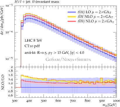
Figure 3: Invariant mass distributions of the $t\bar{t}$-pairs for $t\bar{t}H$ and $t\bar{t}Hj$ at NLO relative to the $t\bar{t}Hj$ at LO for $\mu=2\times\textrm{GA}_{T}$.

The time required for the computation of the full color- and helicity-summed amplitudes in one phase-space point is about $2.5$ seconds. The numerical values of the one-loop amplitudes for the two partonic processes listed in Eq. (1) in a non-exceptional phase-space point are collected in the Appendix.

In view of the later comparison between the processes $pp\to t{\bar{t}}H$ and $pp\to t{\bar{t}}Hj$ at NLO QCD accuracy, we also used the GoSam/Ninja+Sherpa framework to compute the cross section for $t{\bar{t}}H$ production. We found excellent agreement with the results presented in Refs. Hirschi et al. (2011); Frederix et al. (2011).

III Numerical results

In the following, we present results for the integrated cross section for a center-of-mass energy of $8$ TeV. The mass of the Higgs boson is set to $m_{H}=126$ GeV and the top quark mass is set to $m_{t}=172.5$ GeV. The parameters of the electroweak sector are fixed by setting $M_{W}=80.419$ GeV, $M_{Z}=91.1876$ GeV and $\alpha_{EW}^{-1}=132.50698$.

To cluster the jets we use the antikt-algorithm implemented in FastJet Cacciari and Salam (2006); Cacciari et al. (2008, 2012) with radius $R=0.5$, a minimum transverse momentum of $p_{T,jet}>15$ GeV and pseudorapidity $|\eta|<4.0$. The LO cross sections are computed with the LO parton-distribution functions cteq6L1 Pumplin et al. (2002), whereas at NLO we use CT10 Lai et al. (2010).

In order to study the scale dependence of the total cross section, we employ two different choices of the renormalization and factorization scales $\mu_{R}=\mu_{F}=\mu_{0}$, namely $\mu_{0}=H_{T}$ and $\mu_{0}=2\times\textrm{GA}_{T}$ with

$$H_{T} =\sum_{\tiny{\begin{array}[]{cc}\mbox{\tiny final }\\ \mbox{ \tiny states }f\end{array}}}\left|p_{T,f}\right|\;,$$ (4)

$$\textrm{GA}_{T} =\sqrt[3]{m_{T,H}\,m_{T,t}\,m_{T,\bar{t}}}+\sum_{\tiny{\mbox{\tiny jets }j}}|p_{T,j}|\,.$$ (5)

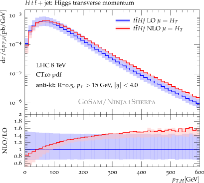
Figure 4: Transverse momentum distribution of the Higgs boson at LO and NLO for $\mu=H_{T}$.

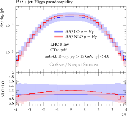
Figure 5: Pseudorapidity $\eta$ of the Higgs boson at LO and NLO accuracy for $\mu=H_{T}$.

Within this setup, for the two scale choices, we obtain the total LO and NLO cross sections reported in Table 1.

Central Scale	$\sigma_{LO}$ [fb]	$\sigma_{NLO}$ [fb]
2$\times\textrm{GA}_{T}$	$80.03^{+35.64}_{-23.02}$	$100.6^{+0.00}_{-9.43}$
$H_{T}$	$88.93^{+41.41}_{-26.13}$	$102.3^{+0.00}_{-15.82}$

Table 1: Total cross section for $t\bar{t}Hj$ for different choices of the central scale at LO and NLO.

The scale dependence of the total cross section, depicted in Fig. 2, is strongly reduced by the inclusion of the NLO contributions. It is worthwhile to notice that both choices for the central value of the scale provide an adequate description, being close to the physical scale of the process.

In Fig. 3, we compare the distributions for the invariant mass of the top quark pair in $pp\to t{\bar{t}}Hj$ at LO and NLO with the NLO curve for $pp\to t{\bar{t}}H$. For $t{\bar{t}}Hj$, going from LO to NLO accuracy, we observe an increase in the distribution by 20–35% over the full kinematical range. On the other hand, when comparing the NLO $t{\bar{t}}H$ prediction with the NLO $t{\bar{t}}Hj$ curve, the cross section decreases due to the presence of the additional jet which takes away energy from the $t\bar{t}$ system. This is particularly evident near the $t\bar{t}$ production threshold, while for high values of the $t{\bar{t}}$ invariant mass the two NLO curves get closer. The scale for this comparison is set to $\mu=2\times\textrm{GA}_{T}$.

In Fig. 4 and Fig. 5, we display the distributions of the transverse momentum $p_{T}$ and the pseudorapidity $\eta$ of the Higgs boson, respectively. Each plot contains the distributions at LO and NLO accuracy, for a value of the scale set to $\mu=H_{T}$. The NLO corrections are particularly important for high values of the $p_{T}$, which are the kinematical regions involved in the boosted analyses Butterworth et al. (2008); Plehn et al. (2010).

These distributions show the potential of the framework obtained combining GoSam/Ninja with Sherpa, which can be successfully used to compute NLO predictions for multi-leg processes involving massive particles. Moreover they shed some light on the impact of further jet activity in $pp\to t\bar{t}H$, one of the most important processes for the direct determination of the coupling of the Higgs boson to fermions. The NLO QCD corrections reduce the scale uncertainty and their numerical impact can be sizable. Therefore they could be helpful for an accurate simulation of the signal in the experimental searches looking for Higgs production in association with a top-antitop pair at the LHC.

Acknowledgments –

We thank all the other members of the GoSam project for collaboration on the common development of the code. We also thank Jan Winter for interesting discussions. The work of H.v.D., G.L., P.M., and T.P. was supported by the Alexander von Humboldt Foundation, in the framework of the Sofja Kovaleskaja Award Project “Advanced Mathematical Methods for Particle Physics”, endowed by the German Federal Ministry of Education and Research. G.O. was supported in part by the National Science Foundation under Grant PHY-1068550. Computing resources were provided by the CTP cluster of the New York City College of Technology.

*

Appendix A Benchmark phase-space point

In this appendix we collect numerical results for the renormalized virtual contributions to the processes (1), in correspondence to the phase-space point in Table 2. The results are collected in Table 3 and are computed using dimensional reduction. The coefficients $a_{i}$ are defined as follows:

$$\frac{a_{-2}}{\epsilon^{2}}+\frac{a_{-1}}{\epsilon}+a_{0}\equiv\frac{2\mathfrak{Re}\left\{\mathcal{M}^{\mbox{\tiny tree-level}\ast}\mathcal{M}^{\mbox{\tiny one-loop}}\right\}}{(\alpha_{s}/2\pi)\left|\mathcal{M}^{\mbox{\tiny tree-level}}\right|^{2}}\,.$$

The reconstruction of the renormalized pole can be checked against the value of $a_{-1}$ and $a_{-2}$ obtained by the universal singular behavior of the dimensionally regularized one-loop amplitudes Catani et al. (2001), while the precision of the finite parts is estimated by re-evaluating the amplitudes for a set of momenta rotated by an arbitrary angle about the axis of collision.

particle	$E$	$p_{x}$	$p_{y}$	$p_{z}$
$p_{1}$	250.00000000000000	0.0000000000000000	0.0000000000000000	250.00000000000000
$p_{2}$	250.00000000000000	0.0000000000000000	0.0000000000000000	-250.00000000000000
$p_{3}$	177.22342332868467	-31.917865771774753	-19.543909461587205	-15.848571666570733
$p_{4}$	174.89951284907735	13.440699620020803	24.174898117950033	-8.2771667589629576
$p_{5}$	126.37478917634435	6.8355633672742222	-3.2652801590882752	6.0992096455298030
$p_{6}$	21.502274645893632	11.641602784479652	-1.3657084972745175	18.026528780003872

Table 2: Benchmark phase-space point for $t\bar{t}Hj$ production

	$q\bar{q}\to t\bar{t}Hg$	$gg\to t\bar{t}Hg$
$a_{0}$	-80.40233474207548	-45.69793352903498
$a_{-1}$	-32.69029102067917	-35.92174974453633
$a_{-2}$	-5.666666666667901	-9.000000000006723

Table 3: Numerical results for the two subprocesses listed in Eq. (1) evaluated at the phase-space point of Table 2 for a scale $\mu=2p_{1}\cdot p_{2}=500$ GeV. The accuracy of the result is indicated by the underlined digits.

References

- Aad et al. (2012) G. Aad et al. (ATLAS Collaboration), Phys.Lett. B716, 1 (2012), eprint 1207.7214.
- Chatrchyan et al. (2012) S. Chatrchyan et al. (CMS Collaboration), Phys.Lett. B716, 30 (2012), eprint 1207.7235.
- CMS-PAS-HIG-13- (005) CMS-PAS-HIG-13-005 (2013).
- Aad et al. (2013) G. Aad et al. (ATLAS Collaboration) (2013), eprint 1307.1427.
- Aaltonen et al. (2013) T. Aaltonen et al. (CDF Collaboration, D0 Collaboration) (2013), eprint 1303.6346.
- Heinemeyer et al. (2013) S. Heinemeyer et al. (The LHC Higgs Cross Section Working Group) (2013), eprint 1307.1347.
- Frederix et al. (2011) R. Frederix, S. Frixione, V. Hirschi, F. Maltoni, R. Pittau, et al., Phys.Lett. B701, 427 (2011), eprint 1104.5613.
- Degrande et al. (2012) C. Degrande, J. Gerard, C. Grojean, F. Maltoni, and G. Servant, JHEP 1207, 036 (2012), eprint 1205.1065.
- Artoisenet et al. (2013) P. Artoisenet, P. de Aquino, F. Maltoni, and O. Mattelaer (2013), eprint 1304.6414.
- Beenakker et al. (2001) W. Beenakker, S. Dittmaier, M. Kramer, B. Plumper, M. Spira, et al., Phys.Rev.Lett. 87, 201805 (2001), eprint hep-ph/0107081.
- Beenakker et al. (2003) W. Beenakker, S. Dittmaier, M. Kramer, B. Plumper, M. Spira, et al., Nucl.Phys. B653, 151 (2003), eprint hep-ph/0211352.
- Dawson et al. (2003a) S. Dawson, L. Orr, L. Reina, and D. Wackeroth, Phys.Rev. D67, 071503 (2003a), eprint hep-ph/0211438.
- Dawson et al. (2003b) S. Dawson, C. Jackson, L. Orr, L. Reina, and D. Wackeroth, Phys.Rev. D68, 034022 (2003b), eprint hep-ph/0305087.
- Dittmaier et al. (2004) S. Dittmaier, . Kramer, Michael, and M. Spira, Phys.Rev. D70, 074010 (2004), eprint hep-ph/0309204.
- Plehn et al. (2010) T. Plehn, G. P. Salam, and M. Spannowsky, Phys.Rev.Lett. 104, 111801 (2010), eprint 0910.5472.
- Mastrolia et al. (2012) P. Mastrolia, E. Mirabella, and T. Peraro, JHEP 1206, 095 (2012), eprint 1203.0291.
- Gleisberg et al. (2009) T. Gleisberg, S. Hoeche, F. Krauss, M. Schonherr, S. Schumann, et al., JHEP 0902, 007 (2009), eprint 0811.4622.
- Krauss et al. (2002) F. Krauss, R. Kuhn, and G. Soff, JHEP 0202, 044 (2002), eprint hep-ph/0109036.
- Catani et al. (2002) S. Catani, S. Dittmaier, M. H. Seymour, and Z. Trocsanyi, Nucl.Phys. B627, 189 (2002), eprint hep-ph/0201036.
- Gleisberg and Krauss (2008) T. Gleisberg and F. Krauss, Eur.Phys.J. C53, 501 (2008), eprint 0709.2881.
- Cullen et al. (2012) G. Cullen, N. Greiner, G. Heinrich, G. Luisoni, P. Mastrolia, et al., Eur.Phys.J. C72, 1889 (2012), eprint 1111.2034.
- Nogueira (1993) P. Nogueira, J.Comput.Phys. 105, 279 (1993).
- Vermaseren (2000) J. A. M. Vermaseren (2000), eprint math-ph/0010025.
- Reiter (2010) T. Reiter, Comput.Phys.Commun. 181, 1301 (2010), eprint 0907.3714.
- Cullen et al. (2011a) G. Cullen, M. Koch-Janusz, and T. Reiter, Comput.Phys.Commun. 182, 2368 (2011a), eprint 1008.0803.
- Kuipers et al. (2013) J. Kuipers, T. Ueda, J. Vermaseren, and J. Vollinga, Comput.Phys.Commun. 184, 1453 (2013), eprint 1203.6543.
- Ossola et al. (2007a) G. Ossola, C. G. Papadopoulos, and R. Pittau, Nucl.Phys. B763, 147 (2007a), eprint hep-ph/0609007.
- Ossola et al. (2007b) G. Ossola, C. G. Papadopoulos, and R. Pittau, JHEP 0707, 085 (2007b), eprint 0704.1271.
- Ellis et al. (2008) R. K. Ellis, W. T. Giele, and Z. Kunszt, JHEP 03, 003 (2008), eprint 0708.2398.
- Ossola et al. (2008) G. Ossola, C. G. Papadopoulos, and R. Pittau, JHEP 0805, 004 (2008), eprint 0802.1876.
- Mastrolia et al. (2008) P. Mastrolia, G. Ossola, C. Papadopoulos, and R. Pittau, JHEP 0806, 030 (2008), eprint 0803.3964.
- Mastrolia et al. (2010) P. Mastrolia, G. Ossola, T. Reiter, and F. Tramontano, JHEP 1008, 080 (2010), eprint 1006.0710.
- Heinrich et al. (2010) G. Heinrich, G. Ossola, T. Reiter, and F. Tramontano, JHEP 1010, 105 (2010), eprint 1008.2441.
- van Hameren (2011) A. van Hameren, Comput.Phys.Commun. 182, 2427 (2011), eprint 1007.4716.
- Binoth et al. (2010) T. Binoth, F. Boudjema, G. Dissertori, A. Lazopoulos, A. Denner, et al., Comput.Phys.Commun. 181, 1612 (2010), eprint 1001.1307.
- van Deurzen et al. (2013) H. van Deurzen, N. Greiner, G. Luisoni, P. Mastrolia, E. Mirabella, et al., Phys.Lett. B721, 74 (2013), eprint 1301.0493.
- Cullen et al. (2013) G. Cullen, H. van Deurzen, N. Greiner, G. Luisoni, P. Mastrolia, et al., Phys.Rev.Lett. 111, 131801 (2013), eprint 1307.4737.
- Maltoni and Stelzer (2003) F. Maltoni and T. Stelzer, JHEP 0302, 027 (2003), eprint hep-ph/0208156.
- Frederix et al. (2008) R. Frederix, T. Gehrmann, and N. Greiner, JHEP 0809, 122 (2008), eprint 0808.2128.
- Frederix et al. (2010) R. Frederix, T. Gehrmann, and N. Greiner, JHEP 1006, 086 (2010), eprint 1004.2905.
- Hoeche et al. (2013) S. Hoeche, J. Huang, G. Luisoni, M. Schoenherr, and J. Winter, Phys.Rev. D88, 014040 (2013), eprint 1306.2703.
- Forde (2007) D. Forde, Phys. Rev. D75, 125019 (2007), eprint 0704.1835.
- Kilgore (2007) W. B. Kilgore (2007), eprint 0711.5015.
- Badger (2009) S. D. Badger, JHEP 01, 049 (2009), eprint 0806.4600.
- Catani et al. (2001) S. Catani, S. Dittmaier, and Z. Trocsanyi, Phys.Lett. B500, 149 (2001), eprint hep-ph/0011222.
- Binoth et al. (2009) T. Binoth, J.-P. Guillet, G. Heinrich, E. Pilon, and T. Reiter, Comput.Phys.Commun. 180, 2317 (2009), eprint 0810.0992.
- Cullen et al. (2011b) G. Cullen, J. Guillet, G. Heinrich, T. Kleinschmidt, E. Pilon, et al., Comput.Phys.Commun. 182, 2276 (2011b), eprint 1101.5595.
- Hirschi et al. (2011) V. Hirschi, R. Frederix, S. Frixione, M. V. Garzelli, F. Maltoni, et al., JHEP 1105, 044 (2011), eprint 1103.0621.
- Cacciari and Salam (2006) M. Cacciari and G. P. Salam, Phys.Lett. B641, 57 (2006), eprint hep-ph/0512210.
- Cacciari et al. (2008) M. Cacciari, G. P. Salam, and G. Soyez, JHEP 0804, 063 (2008), eprint 0802.1189.
- Cacciari et al. (2012) M. Cacciari, G. P. Salam, and G. Soyez, Eur.Phys.J. C72, 1896 (2012), eprint 1111.6097.
- Pumplin et al. (2002) J. Pumplin, D. Stump, J. Huston, H. Lai, P. M. Nadolsky, et al., JHEP 0207, 012 (2002), eprint hep-ph/0201195.
- Lai et al. (2010) H.-L. Lai, M. Guzzi, J. Huston, Z. Li, P. M. Nadolsky, et al., Phys.Rev. D82, 074024 (2010), eprint 1007.2241.
- Butterworth et al. (2008) J. M. Butterworth, A. R. Davison, M. Rubin, and G. P. Salam, Phys.Rev.Lett. 100, 242001 (2008), eprint 0802.2470.