An Optimization Framework to Improve 4D-Var Data Assimilation System Performance

Abstract

This paper develops a computational framework for optimizing the parameters of data assimilation systems in order to improve their performance. The approach formulates a continuous meta-optimization problem for parameters; the meta-optimization is constrained by the original data assimilation problem. The numerical solution process employs adjoint models and iterative solvers. The proposed framework is applied to optimize observation values, data weighting coefficients, and the location of sensors for a test problem. The ability to optimize a distributed measurement network is crucial for cutting down operating costs and detecting malfunctions.

1 Introduction

Data assimilation improves our understanding of natural phenomena by integrating measurements of the physical system with computer-generated predictions. Important theoretical and practical questions regarding the optimal strategies for collecting the data, and for incorporating it such as to obtain the maximum informational benefit, are yet to be answered. This paper develops a computational framework for improving the performance of data assimilation systems by optimally configuring various parameters of the measuring network. The methodology developed herein has applicability to many other inverse problems and dynamic data driven applications.

The research is carried out in the context of ‘‘four-dimensional variational’’ (4D-Var) data assimilation, arguably the most advanced framework for assimilating observations distributed in time and space with predictions performed with nonlinear numerical models. 4D-Var is extensively used in meteorology, climatology, hydrology and other environmental studies [1, 2, 3, 4, 5]. In the 4D-Var approach the data assimilation problem is posed as a PDE-constrained nonlinear optimization problem, where model states and parameters are tuned in order to obtain predictions that fit best the measurements. In this work the strategies used to collect and process the data are considered to be parameters of the 4D-Var data assimilation system, and are themselves improved via an additional optimization process.

Previous related research has been motivated by the need to quantify the contribution of various 4D-Var parameters on the performance of the system. The fastest directions of state error growth have been identified with the help of singular vectors [6, 7]. In order to quantify the amount of information carried by each individual data point, information theory [8, 9] or statistical design [10] methodologies have been used. An adjoint-sensitivity analysis approach has been employed to assess the contributions of individual observations to reducing forecast errors (observation impact) [11, 12, 13]. These methods have been used to qualitatively guide targeting strategies for adaptive observations [14, 15]. The optimal configuration of observing networks has proved to be very challenging challenging even for the simpler problem of state-estimation [16]. For data assimilation, optimal sensor configuration problem was only partially solved using concepts from control theory such as observability [17]. Observing system simulation experiments [18, 19] offer an ad-hoc solution by searching for good network configurations though the entire set of all possible ones.

This research advances the current state of science by developing a systematic approach to tune various 4D-Var parameters in order to improve the performance of the data assimilation system. The proposed framework defines a ‘‘meta’’-optimization problem on top of the 4D-Var solution. The meta-problem seeks finds the optimal parameter values with respect to a performance functional, and is constrained by another optimization problem -- the 4D-Var. The numerical solution process utilizes the 4D-Var sensitivity equations [20, 21, 22]; to the best of our knowledge the present work is the first study to employ this approach. We illustrate the application of the proposed framework to find optimal observation values, observation weights, and sensor locations. The proposed framework is general and can be employed to meta-optimize any other parameters of a 4D-Var data assimilation system.

The paper is structured as follows. Section 2 reviews the formulation of the 4D-Var data assimilation problem, and the associated sensitivity equations. Section 3 constructs the new optimization based framework for improving the data assimilation system. Numerical results obtained with the two-dimensional shallow water equations illustrate the applicability of the framework in Section 4. Conclusions and directions for future research are provided in Section 5.

2 4D-Var Data Assimilation

In this section we review the 4D-Var data assimilation problem formulation [2, 23, 24, 25, 26], and the sensitivity equations of the 4D-Var solution with respect to various system parameters [21]. These elements provide the building blocks for optimizing the data assimilation system, including the sensor network configuration.

2.1 Formulation

Data assimilation (DA) combines three sources of information: a priori estimates on the system states (‘‘background’’), knowledge of the governing physical laws (‘‘model’’), and measurements of the real system (‘‘observations’’). The three sources of information are reconciled through a series of computational steps in order to generate improved (‘‘analyzed’’) estimates of the model states or model parameters.

4D-Var data assimilation takes a Bayesian approach and seeks maximum likelihood estimates of these values with respect to the posterior probability density (conditioned by observations). 4D-Var assimilation is formulated as a PDE-constrained nonlinear optimization problem where the analysis (the most likely initial state) $\mathbf{x}^{\rm a}_{0}$ is obtained by minimizing the following (negative log-likelihood) cost function:

$$\mathcal{J}(\mathbf{x}_{0}) = \frac{1}{2}\left(\mathbf{x}_{0}-\mathbf{x}^{\rm b}_{0}\right)^{T}\cdot\mathbf{B}_{0}^{-1}\cdot(\mathbf{x}_{0}-\mathbf{x}^{\rm b}_{0})$$

$$\,+\frac{1}{2}\sum_{k=0}^{N}\left(\mathcal{H}_{k}(\mathbf{x}_{k})-\mathbf{y}_{k}\right)^{T}\cdot\mathbf{R}_{k}^{-1}\cdot\left(\mathcal{H}_{k}(\mathbf{x}_{k})-\mathbf{y}_{k}\right)\,,$$

$$\mathbf{x}^{\rm a}_{0} = \arg\min_{\mathbf{x}_{0}}\mathcal{J}(\mathbf{x}_{0})\quad\textnormal{subject to }\mathbf{x}_{k}=\mathcal{M}_{t_{0}\rightarrow t_{k}}(\mathbf{x}_{0})\,.$$ (1b)

Here $\mathcal{M}_{t_{0}\rightarrow t_{k}}$ represents the numerical model used to evolve the initial state vector $\mathbf{x}_{0}$ to future times $t_{k}$, $k=0,\dots,N$. This is called the forward model (fwd) or forecast model. $\mathcal{H}_{k}$ is the observation operator which maps the model state $\mathbf{x}_{k}\approx\mathbf{x}(t_{k})$ onto the observation space. The error covariance matrices $\mathbf{B}_{0}$ and $\mathbf{R}_{k}$ quantify the uncertainty in the background state ($\mathbf{x}^{\rm b}_{0}$) and in the observations ($\mathbf{y}_{k}$ for each $t_{k}$), respectively; they are prescribed by the user and their choice influences the quality of the resulting analysis.

The name ‘‘four-dimensional’’ indicates that the method operates with time-distributed observations. When assimilating observations only at the initial time $t_{0}$, the method is known as ‘‘three-dimensional variational’’ (3D-Var), as the additional time dimension is not present.

2.2 Numerical solution

The analysis (initial) state $\mathbf{x}^{\rm a}_{0}$ is the unconstrained minimizer of (1b) and satisfies the first-order optimality condition:

$$\nabla_{\mathbf{x}_{0}}\,\mathcal{J}(\mathbf{x}^{\rm a}_{0})=\mathbf{B}_{0}^{-1}\left(\mathbf{x}^{\rm a}_{0}-\mathbf{x}^{\rm b}_{0}\right)+\sum_{k=0}^{N}\mathbf{M}_{0,k}^{T}\mathbf{H}_{k}^{T}\mathbf{R}_{k}^{-1}\left(\mathcal{H}_{k}(\mathbf{x}^{\rm a}_{k})-\mathbf{y}_{k}\right)=0\,,$$ (2)

where $\mathbf{M}_{0,k}=\mathcal{M}_{t_{0}\rightarrow t_{k}}^{\prime}(\mathbf{x}_{0})$ is the tangent linear propagator associated with the numerical model $\mathcal{M}$, while $\mathbf{M}^{T}_{0,k}$ represets its adjoint counterpart. $\mathbf{H}_{k}=\mathcal{H}_{k}^{\prime}(\mathbf{x}_{k})$ is the linearized observation operator at time $t_{k}$.

The minimizer $\mathbf{x}^{\rm a}_{0}$ is computed numerically using gradient-based methods such as quasi-Newton [27], nonlinear conjugate gradients [28], or truncated Newton [29]. These methods require the derivatives of $\mathcal{J}$ to the initial model states $\mathbf{x}_{0}$, which can be computed using the methodology of adjoint models [24, 25]. Adjoint models have been successfully implemented in optimization, sensitivity analysis and uncertainty quantification [26, 30, 31]. In previous research we have constructed adjoint models of order up to two and have compare the performance of different gradient-based optimization algorithm for solving (1b) [31].

2.3 Sensitivity equations

Using the framework of sensitivity analysis and adjoint models, one can compute how small changes in the data assimilation parameters translate into changes in the resulting analysis. The derivation below follows the 4D-Var sensitivity approach of Daescu [21].

Consider the 4D-Var problem (1b) where cost function $\mathcal{J}$ depends on a vector of parameters $\mathbf{u}\in\mathbb{R}^{m}$:

$$\mathbf{x}^{\rm a}_{0}(\mathbf{u})=\arg\min_{\mathbf{x}_{0}}\mathcal{J}(\mathbf{x}_{0},\mathbf{u})\quad\textnormal{subject to }\mathbf{x}_{k}=\mathcal{M}_{t_{0}\rightarrow t_{k}}(\mathbf{x}_{0},\mathbf{u})\,.$$

The optimal solution $\mathbf{x}^{\rm a}_{0}$ satisfies the first order optimality condition for any $\bar{\mathbf{u}}$:

$$\nabla_{\mathbf{x}_{0}}\,\mathcal{J}\left(\mathbf{x}^{\rm a}_{0}(\bar{\mathbf{u}}),\bar{\mathbf{u}}\right)=0\,.$$ (3)

The 4D-Var Hessian is positive definite at the optimum, $\nabla_{\mathbf{x}_{0},\mathbf{x}_{0}}^{2}\mathcal{J}(\mathbf{x}^{\rm a}_{0}(\bar{\mathbf{u}}),\bar{\mathbf{u}})>0$. The implicit function theorem [32] applied to (3) guarantees that there exists a neighborhood of $\bar{\mathbf{u}}$ where the optimal solution $\mathbf{x}^{\rm a}_{0}(\mathbf{u})$ is a smooth function of the parameters, and

$$\nabla_{\mathbf{u}}\,\mathbf{x}^{\rm a}_{0}(\mathbf{u})=-\nabla_{\mathbf{u},\mathbf{x}_{0}}^{2}\mathcal{J}(\mathbf{x}^{\rm a}_{0}(\mathbf{u}),\mathbf{u})\cdot\left(\nabla_{\mathbf{x}_{0},\mathbf{x}_{0}}^{2}\mathcal{J}(\mathbf{x}^{\rm a}_{0}(\mathbf{u}),\mathbf{u})\right)^{-1}\,.$$ (4)

The gradient of the analysis to the set of parameters is the negative product between the gradient of the first-order optimality condition with respect to the set of parameters, and the inverse of the 4D-Var Hessian with respect to model states.

In our previous research we have developed methods to compute efficiently the sensitivity to observations and the ‘‘observation impact’’ using second-order adjoint models, preconditioners [33], and low-rank approximations based on the singular value decomposition [34].

A complete set of sensitivity equations for observations, observation covariances, background and background covariances can be found in the original derivation of Daescu [21]. Each of the three applications presented later in this paper requires a different sensitivity equation, which is provided along with the description of the problem.

3 Improving the 4D-Var Data Assimilation System via Continuous Optimization

This section develops a methodology to improve the performance of the 4D-Var data assimilation system by optimizing the system parameters with respect to a certain objective. Our specific goal in this paper is to enhance the observing network, but other aspects of the system can be treated in a similar manner. The proposed continuous optimization approach is general, elegant, and easy to implement, since it reuses the same adjoint models and numerical libraries employed for solving the 4D-Var problem.

3.1 General formulation of the parameter optimization problem

The first step in defining the optimization problem is to choose the aspects of the data assimilation system that one seeks to improve. The objective function is a metric defined on the analysis (the output of the assimilation system). The optimization process finds the values of a set of system parameters which minimize (or maximize) the chosen metric. In a continuous optimization setting the objective function must be defined over a continuous space, where additional constraints can also be imposed.

Many data assimilation studies [15, 11, 21] quantify the performance of the 4D-Var system by the discrepancy between the model forecast (initialized from the analysis $\mathbf{x}^{\rm a}_{0}$) at verification time $t_{v}$ and a verification forecast $\mathbf{x}^{\rm verif}_{v}$, defined at the same time. The verification $\mathbf{x}^{\rm verif}_{v}$ represents a control (reference) estimate of the true state. The magnitude of this discrepancy can be measured by the quadratic ‘‘verification’’ cost function

$$\Psi(\mathbf{u})=\Psi\bigl{(}\mathbf{x}^{\rm a}_{v}(\mathbf{u})\bigr{)}=\frac{1}{2}\left(\mathbf{x}^{\rm a}_{v}(\mathbf{u})-\mathbf{x}^{\rm verif}_{v}\right)^{T}\,\mathbf{C}\,\left(\mathbf{x}^{\rm a}_{v}(\mathbf{u})-\mathbf{x}^{\rm verif}_{v}\right)\,.$$ (5)

The weighting matrix $\mathbf{C}$ can be prescribed to scale the error or to restrict it to a certain subdomain. Throughout this paper we take it equal to be the identity matrix, therefore each component of the error vector $(\mathbf{x}^{\rm a}_{v}-\mathbf{x}^{\rm verif}_{v})$ contributes equally towards the value of $\Psi$. The analysis $\mathbf{x}^{\rm a}_{0}$ depends on all sources of information being assimilated: background, observations etc. The function $\Psi$ depends directly on $\mathbf{x}^{\rm a}_{0}(\mathbf{u})$, and therefore depends indirectly on the system parameters $\mathbf{u}$.

The continuous parameter optimization problem seeks the parameter value $\mathbf{u}_{\textrm{opt}}$ which minimizes the verification functional (5)

$$\mathbf{u}_{\textrm{opt}}=\arg\min_{\mathbf{u}}\Psi\bigl{(}\mathbf{x}^{\rm a}_{v}\bigr{)}\quad\textnormal{subject to }\left\{\begin{array}[]{l}\nabla_{\mathbf{x}_{0}}\mathcal{J}\bigl{(}\mathbf{x}^{\rm a}_{0},\mathbf{u}\bigr{)}=0\,,\\[2.0pt] \mathbf{x}^{\rm a}_{v}=\mathcal{M}_{t_{0}\rightarrow t_{v}}(\mathbf{x}^{\rm a}_{0})\,.\end{array}\right.$$ (6)

The optimization problem is constrained by the first order optimality condition (3), which implicitly defines the dependency of the analysis $\mathbf{x}^{\rm a}_{0}(\mathbf{u})$ on the system parameters $\mathbf{u}$, and by the model equations, which relate $\mathbf{x}^{\rm a}_{v}(\mathbf{u})$ to $\mathbf{x}^{\rm a}_{0}(\mathbf{u})$. Note that (6) is an ‘‘optimization-constrained optimization problem’’ with the following equivalent formulation

$$\mathbf{u}_{\textrm{opt}}=\arg\min_{\mathbf{u}}\Psi\bigl{(}\mathbf{x}^{\rm a}_{v}\bigr{)}\quad\textnormal{subject to }\left\{\begin{array}[]{l}\mathbf{x}^{\rm a}_{0}=\arg\min_{\mathbf{x}_{0}}\mathcal{J}\bigl{(}\mathbf{x}_{0},\mathbf{u}\bigr{)}\,,\\[2.0pt] \mathbf{x}^{\rm a}_{v}=\mathcal{M}_{t_{0}\rightarrow t_{v}}(\mathbf{x}^{\rm a}_{0})\,.\end{array}\right.$$ (7)

Gradient-based methods can be employed to solve (6). Each iteration requires computing the value of the cost function $\Psi(\mathbf{x}^{\rm a}_{v})$, which in turn requires solving the 4D-Var optimization problem (1b) to obtain $\mathbf{x}^{\rm a}_{0}$. The two optimization problems (6) and (1b) are nested in an outer loop-inner loop fashion. The inner (4D-Var) optimization (1b) must be solved as accurately as possible in order for the optimality condition constraint in (6) to hold. This requires additional computational effort.

Each outer iteration also requires the gradient of $\Psi$ with respect to $\mathbf{u}$. The first-order optimality condition reads

$$\nabla_{\mathbf{u}}\Psi\bigl{(}\mathbf{x}^{\rm a}_{v}(\mathbf{u}_{\textrm{opt}})\bigr{)}=0\,.$$ (8)

Using chain-rule differentiation on (8):

$$\nabla_{\mathbf{u}}\Psi(\mathbf{x}^{\rm a}_{v}(\mathbf{u})) =\nabla_{\mathbf{u}}\,\mathbf{x}^{\rm a}_{0}(\mathbf{u})\cdot\nabla_{\mathbf{x}_{0}}\,\mathbf{x}^{\rm a}_{v}\cdot\nabla_{\mathbf{x}^{\rm a}_{v}}\Psi(\mathbf{x}^{\rm a}_{v})$$

$$=\nabla_{\mathbf{u}}\,\mathbf{x}^{\rm a}_{0}(\mathbf{u})\cdot\mathbf{M}^{T}_{0,v}\cdot\mathbf{C}\,\left(\mathbf{x}^{\rm a}_{v}-\mathbf{x}^{\rm verif}_{v}\right)$$

$$=-\nabla_{\mathbf{u},\mathbf{x}_{0}}^{2}\mathcal{J}\cdot\left(\nabla_{\mathbf{x}_{0},\mathbf{x}_{0}}^{2}\mathcal{J}\right)^{-1}\cdot\mathbf{M}^{T}_{0,v}\cdot\mathbf{C}\,\left(\mathbf{x}^{\rm a}_{v}-\mathbf{x}^{\rm verif}_{v}\right)\,.$$ (9)

Equation (9) is evaluated as follows. The scaled errors at the verification time $t_{v}$ are propagated backwards in time to $t_{0}$ via the adjoint model. This vector is then multiplied by the sensitivity of the analysis with respect to model parameters (4). Specifically, a linear system with the 4D-Var Hessian matrix is solved, and the result multiplied by the second derivative of the 4D-Var cost function.

The last step in fully defining the metaoptimization problem for the data assimilation system is to specify the system parameters $\mathbf{u}$ that we seek to optimize. In this paper we consider three particular 4D-Var parameters:

1. Observation values: $\mathbf{u}\equiv\mathbf{y}$,

2. Observation error covariance: $\mathbf{u}\equiv\mathbf{R}_{k}^{-1}$, and

3. Observation locations (in 2D space): $\mathbf{u}\equiv(\ell_{x},\ell_{y})$.

Each of the three choices for $\mathbf{u}$ is defined in a continuous space. Measurements can take any value within the allowable range of the observed physical variable. Error covariances are defined from the expected value and standard deviation. Sensor locations represent physical locations in the space domain. Neither one imposes any restrictions in defining the continuous optimization problem.

It is important to note that the verification cost function (5) is not the only metric of the data assimilation system one can seek to improve. Previous work in experimental design to optimize sensor networks for direct state estimation (unconstrained by a PDE system) defines the verification cost function based on the Fisher Information Matrix corresponding to the observations [16]. The objective is to optimize an algebraic aspect of the information matrix, related to its spectrum or determinant. Alternatively, an optimal placement of sensors for data assimilation has been proposed such as to maximize the dynamical system observability [17].

3.2 Optimization of observation values

The first application for our continuous optimization approach is reconstructing the optimal values of assimilated observations, i.e observations that would lead to a 4D-Var analysis as close as possible to the verification $\mathbf{x}^{\rm v}_{0}$. The mismatches between the original dataset and the optimal dataset (“what we should have measured”), are useful to detect faulty sensors or errors in the handling and processing of measurement data.

This is achieved by minimizing the verification cost function $\Psi$ with respect to the values of selected observations:

$$(\mathbf{y}_{k})_{\textrm{opt}}=\arg\min_{\mathbf{y}_{k}}\Psi\bigl{(}\mathbf{x}^{\rm a}_{v}\bigr{)}\quad\textnormal{subject to }\left\{\begin{array}[]{l}\nabla_{\mathbf{x}_{0}}\mathcal{J}\bigl{(}\mathbf{x}^{\rm a}_{0},\mathbf{y}_{k}\bigr{)}=0\,,\\[2.0pt] \mathbf{x}^{\rm a}_{v}=\mathcal{M}_{t_{0}\rightarrow t_{v}}(\mathbf{x}^{\rm a}_{0})\,.\end{array}\right.$$ (10)

A numerical solution requires the gradient of $\Psi$ with respect to observations. Differentiating the optimality condition (2) with respect to $\mathbf{y}_{k}$ gives

$$\nabla_{\mathbf{y}_{k},\mathbf{x}_{0}}^{2}\,\mathcal{J}(\mathbf{x}^{\rm a}_{0})=-\mathbf{R}_{k}^{-1}\,\mathbf{H}_{k}\,\mathbf{M}_{0,k}\,,$$

which is used in (9) to obtain the following expression for the gradient of the verification functional to observations:

$$\nabla_{\mathbf{y}_{k}}\Psi=\mathbf{R}_{k}^{-1}\,\mathbf{H}_{k}\,\mathbf{M}_{0,k}\,\left(\nabla_{\mathbf{x}_{0},\mathbf{x}_{0}}^{2}\mathcal{J}(\mathbf{x}^{\rm a}_{0})\right)^{-1}\,\mathbf{M}^{T}_{0,v}\,\mathbf{C}\,\left(\mathbf{x}^{\rm a}_{v}-\mathbf{x}^{\rm verif}_{v}\right)\,.$$

3.3 Optimization of observation weights

The second application of our framework is the tuning of observation covariances. Each individual data point $(\mathbf{y}_{k})_{(i)}$ has an associated error variance $(\sigma^{2}_{k})_{(i)}$, a scalar value which serves as a weighting coefficient during assimilation. The values of $(\sigma^{2}_{k})_{(i)}$ reflect the level of trust one has in the data. This can be related to sensor accuracy and other characteristics of the measurement process.

We use our framework to obtain the optimal values for the $(\sigma^{2}_{k})_{(i)}$ weights for which the verification cost function $\Psi$ is minimized. The optimized weights are obtained through a dynamic approach that will reflect how the data assimilation process made use of the input data (observations). Smaller standard deviations will be associated to observations which have a significant contribution, while larger standard deviations will reflect redundant or corrupt data. It is expected that the data assimilation problem formulated with the improved weights will provide superior forecasts. In addition, the optimal weight values can be used to configure the sensor scanning strategy in terms of intensity or frequency, or to remove certain measuring instruments from the network.

In the derivation below we assume that observation error covariances at each time instant are diagonal matrices $\mathbf{R}_{k}=\textnormal{diag}\{(\sigma^{2}_{k})_{(i)}\}$. The optimization variables in our formulation are the diagonal elements of all $\mathbf{R}_{k}$, and we seek to compute the optimal values $(\sigma^{2}_{k})_{(i)}$ for which $\Psi$ attains its minimum:

$$(\mathbf{R}_{k})_{\textrm{opt}}=\arg\min_{\mathbf{R}_{k}}\Psi\bigl{(}\mathbf{x}^{\rm a}_{v}\bigr{)}\quad\textnormal{subject to }\left\{\begin{array}[]{l}\nabla_{\mathbf{x}_{0}}\mathcal{J}\bigl{(}\mathbf{x}^{\rm a}_{0},\mathbf{R}_{k}\bigr{)}=0\,,\\[2.0pt] \mathbf{x}^{\rm a}_{v}=\mathcal{M}_{t_{0}\rightarrow t_{v}}(\mathbf{x}^{\rm a}_{0})\,.\end{array}\right.$$ (11)

From the 4D-Var sensitivity equations [21] the gradient of $\Psi$ to $\mathbf{R}_{k}$ is:

$$\nabla_{\mathbf{R}_{k}}\Psi=\left(\mathbf{R}_{k}^{-1}\left[\mathcal{H}(\mathbf{x})-\mathbf{y}\right]\right)\,\otimes\,\nabla_{\mathbf{y}}\Psi(\mathbf{R}_{k})\,,$$ (12)

where the operator $\otimes$ denotes the Kronecker matrix product, and the expression (12) holds for non-diagonal $\mathbf{R}_{k}$ matrices as well.

Previous studies [22] have performed background and error covariance tuning by parameterizing the error covariance matrices as

$$\mathbf{B}_{0}(s_{0})=s_{0}\cdot\mathbf{B}_{0},\qquad\mathbf{R}_{k}(s_{k})=s_{k}\cdot\mathbf{R}_{k}\,,$$

and by optimizing the scaling parameters $s_{0}$ and $s_{k}$ such that more weight is associated either to the background or to the observations.

Our approach differentiates between individual observation weights and optimizes for each component of $\mathbf{R}_{k}$. Based on (12) the optimization problem (11) can be formulated and solved for non diagonal observation error covariances as well.

3.4 Optimization of observation locations

The third application of our optimization framework is finding the optimal locations for the sensors.

In a real data assimilation system observations are available at a sparse set of preselect locations where the measuring instruments are installed. We consider the case where the measured quantities correspond to computed variables in the model. The observation operator $\mathcal{H}$ (1) interpolates the model solution $\mathbf{x}_{k}$ in physical space to the locations of the sensors measuring $\mathbf{y}_{k}$. Each component of the observation vector $\mathbf{y}_{k}$ is associated with its location in physical space, e.g., in two dimensions identified by the Cartesian coordinates $(\ell_{x},\ell_{y})$. Similarly, each component $\mathbf{z}_{i}$ of the model solution $\mathbf{z}\equiv\mathbf{x}_{k}$ is associated with a grid point with coordinates $(\ell_{x_{i}},\ell_{y_{i}})$.

The formulation of the interpolation operator $\mathcal{H}_{k}$ explicitly contains the coordinates of the sensor locations (i.e. of the points where interpolation is performed). Therefore the 4D-Var cost function $\mathcal{J}$, and the analysis $\mathbf{x}^{\rm a}_{0}$, both depend on these locations. We denote the set of all sensor locations within the assimilation window by

$$L=\bigcup_{\rm all~{}sensors}\{(\ell_{x},\ell_{y},t_{k})\}\,.$$

The sensor location optimization problem is formulated as follows:

$$L_{\textrm{opt}} =\arg\min_{\ell_{x},\ell_{y}}\Psi\bigl{(}L)\quad\textnormal{subject to }\left\{\begin{array}[]{l}\nabla_{\mathbf{x}_{0}}\mathcal{J}\bigl{(}\mathbf{x}^{\rm a}_{0},L\bigr{)}=0\,,\\[2.0pt] \mathbf{x}^{\rm a}_{v}=\mathcal{M}_{t_{0}\rightarrow t_{v}}(\mathbf{x}^{\rm a}_{0})\,.\end{array}\right.$$ (15)

In this study we choose the Inverse Distance Weighting (IDW) [35] interpolant as the $\mathcal{H}_{k}$ operator. We apply it to the spatial locations only and do not attempt to optimize for the time distribution of measurements. IDW is a general scheme and is very popular in geographic information systems and climate modeling.

IDW interpolates the model solution values $\mathbf{z}_{i}$ through a linear combination of all available data points, each weighted by their inverse distance to the interpolation location. For each interpolation location $(\ell_{x},\ell_{y})$ we have

$$\mathcal{H}_{k}(\ell_{x},\ell_{y};\mathbf{z})=\left\{\begin{array}[]{cl}\displaystyle\frac{\sum\limits_{i}d_{i}^{-1}\,\mathbf{z}_{i}}{\sum\limits_{i}d_{i}^{-1}},&\textnormal{if }d_{i}\neq 0\,,\\ \mathbf{z}_{i},&\textnormal{if }d_{i}=0\,,\end{array}\right.$$ (18)

$$\textnormal{where }d_{i}=\left[\left(\ell_{x}-\ell_{x_{i}}\right)^{2}+\left(\ell_{y}-\ell_{y_{i}}\right)^{2}\right]^{1/2}\,.$$

Differentiation of the first order optimality condition of 4D-Var (2) yields

$$\nabla_{\ell_{x},\mathbf{x}_{0}}^{2}\mathcal{J} = \nabla_{\ell_{x}}\mathcal{H}_{k}(\ell_{x},\ell_{y};\mathbf{x}^{\rm a}_{k})$$

$$+\mathbf{M}_{0,k}^{T}\,\left(\nabla_{\ell_{x}}\mathbf{H}_{k}(\ell_{x},\ell_{y};\mathbf{x}^{\rm a}_{k})\right)^{T}\,\mathbf{R}_{k}^{-1}\,\left(\mathcal{H}_{k}(\ell_{x},\ell_{y};\mathbf{x}^{\rm a}_{k})-\mathbf{y}_{k}\right)\,,$$

$$\nabla_{\ell_{y},\mathbf{x}_{0}}^{2}\mathcal{J} = \nabla_{\ell_{y}}\mathcal{H}_{k}(\ell_{x},\ell_{y};\mathbf{x}^{\rm a}_{k})$$

$$+\mathbf{M}_{0,k}^{T}\,\left(\nabla_{\ell_{y}}\mathbf{H}_{k}(\ell_{x},\ell_{y};\mathbf{x}^{\rm a}_{k})\right)^{T}\,\mathbf{R}_{k}^{-1}\left(\mathcal{H}_{k}(\ell_{x},\ell_{y};\mathbf{x}^{\rm a}_{k})-\mathbf{y}_{k}\right)\,.$$

The gradient of $\Psi$ to coordinates $\ell_{x}$ and $\ell_{y}$ is then computed from (9)

$$\nabla_{\ell_{x}}\Psi=\nabla_{\ell_{x},\mathbf{x}_{0}}^{2}\mathcal{J}\cdot\left(\nabla_{\mathbf{x}_{0},\mathbf{x}_{0}}^{2}\mathcal{J}(\mathbf{x}^{\rm a}_{0})\right)^{-1}\,\mathbf{M}^{T}_{0,v}\,\mathbf{C}\,\left(\mathbf{x}^{\rm a}_{v}-\mathbf{x}^{\rm verif}_{v}\right)\,,$$ (20)

$$\nabla_{\ell_{y}}\Psi=\nabla_{\ell_{y},\mathbf{x}_{0}}^{2}\mathcal{J}\cdot\left(\nabla_{\mathbf{x}_{0},\mathbf{x}_{0}}^{2}\mathcal{J}(\mathbf{x}^{\rm a}_{0})\right)^{-1}\,\mathbf{M}^{T}_{0,v}\,\mathbf{C}\,\left(\mathbf{x}^{\rm a}_{v}-\mathbf{x}^{\rm verif}_{v}\right)\,.$$

Differentiation of (18) with respect to $\ell_{x}$, $\ell_{y}$ gives the gradients of $\mathcal{H}_{k}$ with respect to sensor locations:

$$\nabla_{\ell_{x}}\mathcal{H}_{k}(\ell_{x},\ell_{y};\mathbf{z})=\frac{\sum\limits_{i}\sum\limits_{j}(d_{i})^{-2}(d_{j})^{-1}\left(\ell_{x}-\ell_{x_{i}}\right)\mathbf{z}_{i}\left(\mathbf{z}_{i}-\mathbf{z}_{j}\right)}{\left|\sum\limits_{i}(d_{i})^{-1}\right|^{2}}\,,$$

and

$$\nabla_{\ell_{y}}\mathcal{H}_{k}(\ell_{x},\ell_{y};\mathbf{z})=\frac{\sum\limits_{i}\sum\limits_{j}(d_{i})^{-2}(d_{j})^{-1}\left(\ell_{y}-\ell_{y_{i}}\right)\mathbf{z}_{i}\left(\mathbf{z}_{i}-\mathbf{z}_{j}\right)}{\left|\sum\limits_{i}(d_{i})^{-1}\right|^{2}}\,.$$

The innovation vectors $\mathcal{H}_{k}(\ell_{x},\ell_{y};\mathbf{x}^{\rm a}_{k})-\mathbf{y}_{k}$ evaluated at the analysis solution are likely to have small values. For this reason the derivatives (19) are well approximated by the simpler expressions

$$\nabla_{\ell_{x},\mathbf{x}_{0}}^{2}\mathcal{J}\approx\nabla_{\ell_{x}}\mathcal{H}_{k}(\ell_{x},\ell_{y};\mathbf{x}^{\rm a}_{k})\,,\quad\nabla_{\ell_{y},\mathbf{x}_{0}}^{2}\mathcal{J}\approx\nabla_{\ell_{y}}\mathcal{H}_{k}(\ell_{x},\ell_{y};\mathbf{x}^{\rm a}_{k})\,,$$ (21)

which do not require additional adjoint integrations.

4 Applications

We illustrate the proposed metaoptimization approach for the three applications presented in Section 3 using the two dimensional shallow water equations system.

4.1 Test problem

The two-dimensional shallow-water equations (2D swe) [36] approximate the movement of a thin layer of fluid inside a basin:

$$\frac{\partial}{\partial t}h+\frac{\partial}{\partial x}(uh)+\frac{\partial}{\partial y}(vh) = 0$$

$$\frac{\partial}{\partial t}(uh)+\frac{\partial}{\partial x}\left(u^{2}h+\frac{1}{2}gh^{2}\right)+\frac{\partial}{\partial y}(uvh) = 0$$ (22)

$$\frac{\partial}{\partial t}(vh)+\frac{\partial}{\partial x}(uvh)+\frac{\partial}{\partial y}\left(v^{2}h+\frac{1}{2}gh^{2}\right) = 0\;.$$

Here $h(t,x,y)$ is the fluid layer thickness, and $u(t,x,y)$ and $v(t,x,y)$ are the components of the velocity field of the fluid. The gravitational acceleration is denoted by $g$.

We consider on a spatial domain $\Omega=[-3,\,3]^{2}$ (spatial units), and an integration window is $t_{0}=0\leq t\leq t_{\textrm{f}}=0.1$ (time units). Boundary conditions are specified periodic. The space discretization is realized using a finite volume scheme, and the time integration uses a fourth Runge-Kutta scheme, following the method Lax-Wendroff [37]. The model uses a square $q\times q$ uniform spatial discretization grid, which brings the number of model (state) variables to $n=3\,q^{2}$.

Our adjoint models are built using the automatic differentiation tool TAMC [38, 39]. Perturbations are propagated forward in time using the tangent-linear model (tlm), and backwards in time using the first-order adjoint model (foa), which can also efficiently computes the gradient of a cost functional defined on the model states. The product between the Hessian of a cost functional and a user-defined vector can be computed with the second-order adjoint model (soa) [31].

4.2 Data assimilation setting

The 4D-Var system is set up for a simple version of the ‘‘circular dam’’ problem [40]. Where not specified otherwise, the 4D-Var parameters are configured as follows.

The reference initial height field $h$ is a Gaussian bell of a width equal to $10$ gridpoints centered at the midpoint of the grid, and the reference initial velocity vector components are constant $u=v=0$. The physical interpretation is that the front of water falls to the ground ($h$ decreases) under the effect of gravity and creates concentric ripples which propagate towards the boundaries. Figures 1 represent snapshots of the reference trajectory at initial and final time.

The computational grid is square and regular with $q=40$ grid points in each direction, for a total of $4800$ model variables (states). The simulation time interval is set to $0.01$ seconds, using $N=100$ timesteps of size $0.0001$ (time units).

The $h$ component of the a priori estimate (background) $\mathbf{x}^{\rm b}_{0}$ is generated by adding a correlated perturbation to the $h$ reference solution at initial time. The background error covariance $\mathbf{B}_{0}$ corresponds to a standard deviation of $5\%$ of the reference field values. For the $u$ and $v$ components we use white noise to prescribe perturbations. The spatial error correlation uses a Gaussian decay model, with a correlation distance of five.

Synthetic observations are generated at the final time $t_{100}$, by adding random noise to the reference trajectory. Since the observation errors are assumed uncorrelated, the observation error covariance matrix $\mathbf{R}_{100}$ is diagonal. The standard deviation for observation noise is $1\%$ of the largest absolute value of the observations for each variable. We consider observations of all variables at each grid point and the observation operator $\mathcal{H}$ to be linear. The minimization of the 4D-Var cost function is performed with the L-BFGS-B solver [41] using a fixed number of $100$ iterations. For our problem, this guarantees that the analysis is sufficiently close to the minimum.

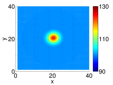
(a) Initial time

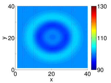
(b) Final time

Figure 1: The height field $h$ at the beginning and at the end of the reference trajectory.

For the verification cost function $\Psi$ we choose $\mathbf{C}$ to be the identity matrix and the verification time $t_{v}=t_{100}$, which corresponds to the final time of our assimilation window. The meta-optimization problems (10), (11), and (15) are also solved using L-BFGS-B [41], which performs 10 ‘‘outer’’ iterations to minimize $\Psi(\mathbf{u})$ with respect to $\mathbf{u}$. Each outer iteration requires the solution of a 4D-Var data assimilation problem, which is obtained by running 100 ‘‘inner iterations’’ of L-BFGS-B to minimize $\mathcal{J}(\mathbf{x}_{0},\mathbf{u})$ with respect to $\mathbf{x}_{0}$.

4.3 Optimization of observation values

This experiment employs the methodology developed in Section 3.2 to correct the values of faulty observations; this is made possible by the redundant information available in the verification functional.

The reference height field $h$ at the initial time is shown in Figure 2(a), and reference solution at the final time $t_{100}$ in Figure 2(b); the latter is used to generate synthetic observations. Assimilation of perfect observations in a twin experiment framework yields an analysis that is close to the reference.

Here we consider the case where some of the observations are corrupted. Specifically, we consider synthetic observations corresponding to the field shown in Figure 3(a). The difference between these corrupted observations and the reference ones (Figure 2(b)) consists in the orientation of the field, now aligned along the perpendicular axis. For example, this could be the result of an indexing mistake when processing large data. Then assimilation of this faulty dataset yields the $h$ analysis shown in Figure 3(b), and is clearly distinct from the reference solution (Figure 2(a)).

We apply the methodology developed in Section 3.2 to define and solve an optimization problem that corrects the observation values $\mathbf{y}_{k}$ such that the 4D-Var analysis becomes more accurate (i.e., closer to the reference).

The initial guess for $\mathbf{y}_{k}$ are the faulty observations from Figure 3(a). We solve the optimization problem (10) using five iterations of L-BFGS [41] and plot the decrease of the cost function values $\Psi(\mathbf{y}_{k})$ at each iteration in Figure 4(a), At first, the error between the 4D-Var analysis and the verification is large, but then it decreases monotonically with each iteration. Most of the cost function decrease happens at the second iteration, with subsequent iterations contributing less significantly to the convergence. The optimal observations computed after five iterations are plotted in Figure 4(b). They are similar to the reference values in Figure 2(b). This validates the approach developed in Section 3.2. Note that the process is computationally efficient, with the optimization converging in less than five iterations. The true error norm corresponding to the reanalyzed initial solution $\mathbf{x}^{\rm a}_{0}$ before and after the optimization is shown in Table 1 and confirms that the 4D-Var process benefits from the new observation values.

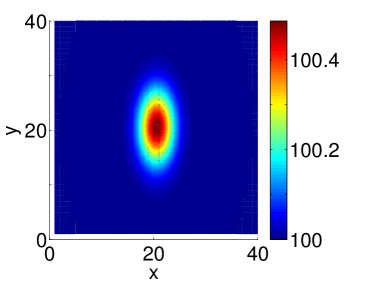
(a) Initial Time

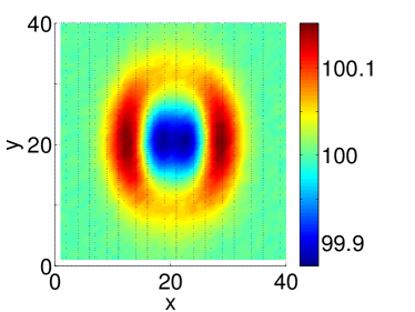
(b) Observation Time

Figure 2: The reference height field $h$ at the initial and final (observation) times.

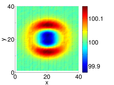
(a) Faulty Observations

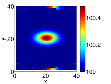
(b) 4D-Var Analysis

Figure 3: The faulty (unoptimized) observations of the height field $h$ and the corresponding 4D-Var analysis.

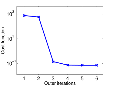
(a) L-BFGS convergence

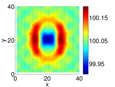
(b) Optimized observation values

Figure 4: The minimization of the verification cost function (10) and the optimized observations at assimilation time $t_{100}$.

Table 1: Error norm of the 4D-Var reanalyzed initial solution before and after optimizing observation values.

	Initial observations	Optimized observations
$\|\mathbf{x}^{\rm a}_{0}-\mathbf{x}_{0}^{\rm reference}\|$	$1.8216$	$0.0703$

4.4 Optimization of observation weights

This experiment illustrates the methodology developed in Section 3.3. In practice measurements contain various amounts of noise, for example due to various sensor accuracies. The observation error covariances specified initially are only rough approximations of the true error statistics. We seek to tune the observation error covariances by solving the optimization problem (11). Improved values of observation error statistics can be obtained by taking advantage of the additional information encapsulated by the verification cost function.

The experiment is set up as follows. We construct a synthetic observational data set for $h$ from the model trajectory at the final time (Figure 5(a)). White noise is added to the perfect values to simulate observational errors. The noise magnitude is nonuniform: it is larger in a contiguous area of rectangular shape, as illustrated in Figure 5(b). Initially the data assimilation system uses the observation error covariance $\mathbf{R}_{k}=\mathbf{I}$. The same noise levels are specified for all grid points, and the data assimilation system is initially unaware of the larger observation errors in the selected area.

Data assimilation using the initially specified error covariances yields the analysis shown in Figure 5(c). This analysis is similar to the reference initial solution (Figure 1), and is not indicative of a misspecification of observation error covariances. The small mismatch, however, can be quantified numerically through the verification functional $\Psi$.

The initial observation variances (diagonal elements of $\mathbf{R}_{k}$) are equal to $1$ (unit), meaning that all data points are equally trusted. We now seek to improve the values of the observation error covariances, and thus improve the performance of the data assimilate system. This is done by solving the optimization problem (11) for the diagonal entries of $\mathbf{R}_{k}$, when the data values $\mathbf{y}$ are fixed.

Five iterations of the numerical optimization solver L-BFGS are performed, and the decrease in the values of $\Psi$ are plotted in Figure 6(a). The solver converges monotonically and achieves a reduction of the verification cost function by a factor of six. The 4D-Var analysis (initial time) is also improved by using the new data weights, as can be shown in Table 2. The optimized values for the observation error variances are plotted in Figure 6(b) (each variance is at the location of the corresponding sensor). The tuned values are considerably larger in the area where observations were perturbed more significantly. and thus the information with high noise levels is given a considerably reduced weight. This result is significant because it shows the possibility to tune the data weights such as to pick up the structure of observational noise, without having direct knowledge of the noise levels.

(a) Perfect Observations

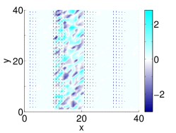
(b) Prescribed Noise (physical variable units)

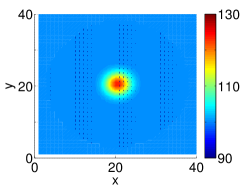
(c) 4D-Var Analysis

Figure 5: The $h$ observations, the prescribed observation noise, and the resulting 4D-Var analysis using the initial specification of the error covariances.

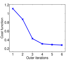
(a) L-BFGS Convergence

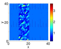
(b) Optimized Covariances

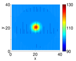
(c) 4D-Var Analysis

Figure 6: The minimization of the verification cost function, the optimized $h$ observation error covariances, and the resulting 4D-Var analysis using the improved values.

The analysis with initial error covariances is shown in Figure 5(c), and the analysis with optimized weights is plotted in Figure 6(c).

Table 2: Error norm of the 4D-Var reanalyzed initial solution before and after optimizing the observation weights.

	Initial weights	Optimized weights
$\|\mathbf{x}^{\rm a}_{0}-\mathbf{x}_{0}^{\rm reference}\|$	$0.4915$	$0.0985$

4.5 Optimization of observation locations

We now apply the methodology developed in Section 3.4 to optimize the spatial configuration of the sensor network such as to improve the performance of the data assimilation system. The approximate gradients (21) are used in the numerical calculations.

This experiment is set up slightly different. The observation network is sparse and consists of $300$ sensors measuring the fluid height $h$. The physical locations of the sensors are specified by a given initial layout; each sensor location is described by its Cartesian coordinates, which can vary continuously within the domain. We change the coordinates of each sensor, i.e., the spatial configuration of the sensor network, by solving the optimization problem (15). The minimization of the verification error translates into an improved performance of the data assimilation system after relocating the observations.

The optimization problem is solved for three scenarios, distinguished by the initial sensor locations. Each scenario starts from an equidistant spatial distribution of sensors, as shown in Figures 7(a), 8(a), and 9(a), respectively. L-BFGS is ran for solving (15) over $30$ iterations, and the corresponding decreases in cost function values for each scenario are plotted in Figures 7(b), 8(b), and 9(b), respectively. We can notice that for the first two scenarios the cost function decrease is converging to a minimum. Meanwhile, the iterative solver broke down for the third scenario after decreasing the cost function within the first $20$ iterations.

The resulting optimal locations for each scenario are shown in Figures 7(c), 8(c), and 9(c), respectively.

In each scenario the optimization adjusts slightly the locations of the sensors; this is sufficient for obtaining a considerable reduction in the verification cost function $\Psi$, i.e., for obtaining a measurable improvement in the data assimilation system performance. Table 3 contains the true error norm of the 4D-Var reanalyzed initial solution for each solution and we can notice corresponding improvements.

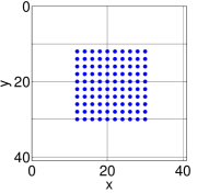
(a) Initial locations

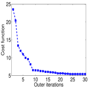
(b) L-BFGS convergence

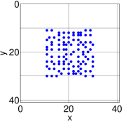
(c) Optimized locations

Figure 7: The optimization of sensor locations for the first testing scenario: initial locations, numerical solver convergence, and optimal locations.

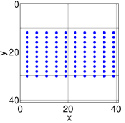
(a) Initial locations

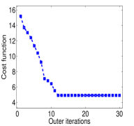
(b) L-BFGS convergence

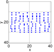
(c) Optimized locations

Figure 8: The optimization of sensor locations for the second testing scenario: initial locations, numerical solver convergence, and optimal locations.

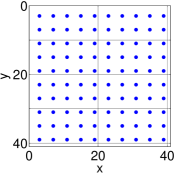
(a) Initial locations

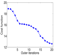
(b) L-BFGS convergence

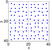
(c) Optimized locations

Figure 9: The optimization of sensor locations for the third testing scenario: initial locations, numerical solver convergence, and optimal locations.

While the performance is improved in each of the three scenarios, the computed solutions are clearly only local minima of (15), located in the vicinity of the corresponding initial configurations. Note that the global optimum coincides for all three cases, and represents the best locations of $300$ sensors within the domain. The convergence to a local optimum is to be expected for the quasi-Newton approach used herein, as the gradients mostly contain information that is locally valid.

Table 3: Error norm of the 4D-Var reanalyzed initial solution before and after optimizing sensor locations.

Assimilation Scenario		Initial locations	Optimized locations
1		$0.3923$	$0.1960$
2	$\|\mathbf{x}^{\rm a}_{0}-\mathbf{x}_{0}^{\rm reference}\|$	$0.3213$	$0.1906$
3		$0.3327$	$0.2897$

5 Conclusions and Future Work

This paper, develops a computational framework for improving the performance of 4D-Var data assimilation systems. The approach is based on optimizing various 4D-Var parameters with respect to a forecast aspect quantified by a verification cost functional. The particular aspect considered here is the norm of a forecast error estimate. System parameters include the observation values, the observation covariances, and the location of sensors.

The verification functional is defined on the analysis, i.e., on the solution of the data assimilation problem. We formulate a constrained continuous optimization problem to find the best parameter values for the data assimilation system. The cost function is the verification functional, and the constraints are the optimality conditions of the 4D-Var system. Thus we have an ‘‘optimization-constrained optimization problem’’. The computational solution employs gradient-based numerical optimization methods. The gradient of the forecast aspect of interest with respect to data assimilation system parameters is computed (relatively) efficiently using adjoint models and the framework of 4D-Var sensitivity analysis. The proposed methodology is the first of its kind and can be readily integrated in data assimilation studies for weather, climate, air-quality and many others.

Our study shows that an optimization problem constrained by the 4D-Var problem itself is tractable and can improve the quality of analyses generated by the data assimilation system. Numerical results obtained with a test shallow water equations system illustrate how the proposed approach successfully optimized the values of observations, observation error covariances, and sensor locations.

This research opens the path for solving a multitude of problems related to the optimal configuration of specific 4D-Var data assimilation systems. Future work will extend the optimization procedure to other parameters of the data assimilation system such as the background covariance and, in the context of weakly constrained 4D-Var, the model error covariances. The approach will benefit from developing more efficient techniques to compute the derivatives and improving the convergence of the optimization process. We plan to consider alternative formulations of the verification cost functional, such as ones based on information theory, and to extend the framework to include mixed integer optimization problems. This will extend the capabilities of the framework to optimize the observing network by turning sensors on or off, or by selecting the best alternatives from a given set of feasible locations.

References

- [1] E. Kalnay. Atmospheric modeling, data assimilation, and predictability. Cambridge University Press, 2003.
- [2] R. Daley. Atmospheric data analysis, volume 2. Cambridge University Press, 1993.
- [3] J. M. Lewis and S. Lakshmivaran. Dynamic data assimilation: A least squares approach. Cambridge University Press, 2006.
- [4] I. M. Navon. Data assimilation for numerical weather prediction: a review. In Data Assimilation for Atmospheric, Oceanic and Hydrologic Applications, pages 21--65. Springer, 2009.
- [5] T. Chai, G. R. Carmichael, Y. Tang, A. Sandu, M. Hardesty, P. Pilewskie, S. Whitlow, E. V. Browell, M. A. Avery, Ph. Nédélec, et al. Four-dimensional data assimilation experiments with international consortium for atmospheric research on transport and transformation ozone measurements. Journal of Geophysical Research: Atmospheres (1984--2012), 112(D12), 2007.
- [6] T. N. Palmer, R. Gelaro, J. Barkmeijer, and R. Buizza. Singular vectors, metrics, and adaptive observations. Journal of the Atmospheric Sciences, 55(4):633--653, 1998.
- [7] W. Liao, A. Sandu, G. R. Carmichael, and T. Chai. Total energy singular vector analysis for atmospheric chemical transport models. Monthly Weather Review, 2005.
- [8] D. Zupanski, A. Y. Hou, S. Q. Zhang, M. Zupanski, C. D. Kummerow, and S. H. Cheung. Applications of information theory in ensemble data assimilation. Quarterly Journal of the Royal Meteorological Society, 133(627):1533--1545, 2007.
- [9] K. Singh, A. Sandu, M. Jardak, K. W. Bowman, and M. Lee. A practical method to estimate information content in the context of 4D-Var data assimilation. SIAM/ASA Journal of Uncertainty Quantification, 1:106--138, 2013.
- [10] L. M. Berliner, Z.-Q. Lu, and C. Snyder. Statistical design for adaptive weather observations. Journal of the Atmospheric Sciences, 56(15):2536--2552, 1999.
- [11] R. Gelaro, Y. Zhu, and R. M. Errico. Examination of various-order adjoint-based approximations of observation impact. Meteorologische Zeitschrift, 16(6):685--692, 2007.
- [12] R. Gelaro and Y. Zhu. Examination of observation impacts derived from observing system experiments (OSEs) and adjoint models. Tellus A, 61(2):179--193, 2009.
- [13] Y. Trémolet. Computation of observation sensitivity and observation impact in incremental variational data assimilation. Tellus A, 60(5):964--978, 2008.
- [14] N. L. Baker and R. Daley. Observation and background adjoint sensitivity in the adaptive observation-targeting problem. Quarterly Journal of the Royal Meteorological Society, 126(565):1431--1454, 2000.
- [15] D. N. Daescu and I. M. Navon. Adaptive observations in the context of 4D-Var data assimilation. Meteorology and Atmospheric Physics, 85(4):205--226, 2004.
- [16] D. Ucinski. Optimal sensor location for parameter estimation of distributed processes. International Journal of Control, 73(13):1235--1248, 2000.
- [17] W. Kang and L. Xu. Optimal placement of mobile sensors for data assimilations. Tellus A, 64, 2012.
- [18] X. Wang, D. M. Barker, C. Snyder, and T. M. Hamill. A hybrid ETKF-3DVAR data assimilation scheme for the WRF model. Part I: Observing system simulation experiment. Monthly Weather Review, 136(12):5116--5131, 2008.
- [19] R. Atlas. Atmospheric observations and experiments to assess their usefulness in data assimilation. Journal of the Meteorological Society of Japan, 75(1 B):111--130, 1997.
- [20] F.-X. Le Dimet, H. E. Ngodock, B. Luong, and J. Verron. Sensitivity analysis in variational data assimilation. Journal - Meteorological Society of Japan Series 2, 75:135--145, 1997.
- [21] D. N. Daescu. On the sensitivity equations of four-dimensional variational (4D-Var) data assimilation. Monthly Weather Review, 136(8):3050--3065, 2008.
- [22] D. N. Daescu and R. Todling. Adjoint sensitivity of the model forecast to data assimilation system error covariance parameters. Quarterly Journal of the Royal Meteorological Society, 136(653):2000--2012, 2010.
- [23] E. Kalnay. Atmospheric modeling, data assimilation, and predictability. Cambridge University Press, 2003.
- [24] D. G. Cacuci. Sensitivity theory for nonlinear systems. I. Nonlinear functional analysis approach. Journal of Mathematical Physics, 22:2794, 1981.
- [25] Z. Wang, I. M. Navon, F.-X. Le Dimet, and X. Zou. The second order adjoint analysis: theory and applications. Meteorology and atmospheric physics, 50(1-3):3--20, 1992.
- [26] A. Sandu and L. Zhang. Discrete second order adjoints in atmospheric chemical transport modeling. Journal of Computational Physics, 227(12):5949--5983, 2008.
- [27] J. E. Dennis, Jr and J. J. Moré. Quasi-newton methods, motivation and theory. SIAM review, 19(1):46--89, 1977.
- [28] Y.-H. Dai and Y. Yuan. A nonlinear conjugate gradient method with a strong global convergence property. SIAM Journal on Optimization, 10(1):177--182, 1999.
- [29] T. Schlick and A. Fogelson. TNPACK -- A truncated Newton minimization package for large-scale problems: I. Algorithm and usage. ACM Transactions on Mathematical Software (TOMS), 18(1):46--70, 1992.
- [30] A. Sandu, D. N. Daescu, G. R. Carmichael, and T. Chai. Adjoint sensitivity analysis of regional air quality models. Journal of Computational Physics, 204(1):222--252, 2005.
- [31] A. Cioaca, M. Alexe, and A. Sandu. Second-order adjoints for solving pde-constrained optimization problems. Optimization methods and software, 27(4-5):625--653, 2012.
- [32] S. S. G. Krantz and H. R. Parks. The implicit function theorem: history, theory, and applications. Springer, 2002.
- [33] A. Cioaca, A. Sandu, and E. De Sturler. Efficient methods for computing observation impact in 4D-Var data assimilation. CoRR, abs/1305.5796, 2013.
- [34] A. Cioaca and A. Sandu. Low-rank approximations for computing observation impact in 4D-Var data assimilation. ArXiv e-prints, July 2013.
- [35] D. Shepard. A two-dimensional interpolation function for irregularly-spaced data. In Proceedings of the 1968 23rd ACM national conference, pages 517--524. ACM, 1968.
- [36] D. D. Houghton and A. Kasahara. Nonlinear shallow fluid flow over an isolated ridge. Communications on Pure and Applied Mathematics, 21(1):1--23, 1968.
- [37] R. Liska and B. Wendroff. Composite schemes for conservation laws. SIAM Journal on Numerical Analysis, 35(6):2250--2271, 1998.
- [38] R. Giering. Tangent linear and adjoint model compiler. User Manual, TAMC Version, 4, 1997.
- [39] R. Giering and T. Kaminski. Recipes for adjoint code construction. ACM Transactions on Mathematical Software (TOMS), 24(4):437--474, 1998.
- [40] K. Anastasiou and C.T. Chan. Solution of the 2D shallow water equations using the finite volume method on unstructured triangular meshes. International Journal for Numerical Methods in Fluids, 24(11):1225--1245, 1997.
- [41] C. Zhu, R. H. Byrd, P. Lu, and J. Nocedal. Algorithm 778: L-BFGS-B: Fortran subroutines for large-scale bound-constrained optimization. ACM Transactions on Mathematical Software (TOMS), 23(4):550--560, 1997.