Exact results for the low energy $AdS_{4}\times\mathbb{CP}^{3}$ string theory

Alessandro Fabbri^a, Davide Fioravanti^a, Simone Piscaglia^a and Roberto Tateo^b

^a INFN-Bologna and Dipartimento di Fisica ed Astronomia, Università di Bologna,

Via Irnerio 46, 40126 Bologna, Italy.

^b Dipartimento di Fisica and INFN, Università di Torino,

Via P. Giuria 1, 10125 Torino, Italy.

We derive the Thermodynamic Bethe Ansatz equations for the relativistic sigma model describing the $AdS_{4}\times\mathbb{CP}^{3}$ string II A theory at strong coupling (i.e. in the Alday-Maldacena decoupling limit). The corresponding $Y$-system involves an infinite number of $Y$ functions and is of a new type, although it shares a peculiar feature with the $Y$-system for $AdS_{4}\times\mathbb{CP}^{3}$. A truncation of the equations at level $p$ and a further generalisation to generic rank $N$ allow us an alternative description of the theory as the $N=4$, $p=\infty$ representative in an infinite family of models corresponding to the conformal cosets $(\mathbb{CP}^{N-1})_{p}\times U(1)$, perturbed by a relevant composite field $\phi_{(N,p)}=\phi_{[(\mathbb{CP}^{N-1})_{p}]}\times\phi_{[U(1)]}$ that couples the two independent conformal field theories. The calculation of the ultraviolet central charge confirms the conjecture by Basso and Rej and the conformal dimension of the perturbing operator, at every $N$ and $p$, is obtained using the Y-system periodicity. The conformal dimension of $\phi_{[(\mathbb{CP}^{N-1})_{p}]}$ matches that of the field identified by Fendley while discussing integrability issues for the purely bosonic $\mathbb{CP}^{N-1}$ sigma model.

Keywords: Thermodynamic Bethe Ansatz, Y-system, AdS/CFT, Perturbed CFT.

1 Introduction

The theory of quantum exactly solvable models is currently playing an important role in the study of the gauge/gravity correspondence [1, 2] as many powerful integrable model methods were recently adapted to investigate perturbative and nonperturbative aspects in multicolor QCD [3] and various branches of the $AdS/CFT$ duality [4].

The purpose of this paper is to study, through the Thermodynamic Bethe Ansatz (TBA) [5, 6], the finite-size corrections of the (integrable) two-dimensional $\mathbb{CP}^{N-1}$ quantum sigma model minimally coupled to a massless Dirac fermion plus a Thirring term, as described in [7]. Despite the original $\mathbb{CP}^{N-1}$ model (without the fermion) has been intensively studied, helping physicists with its underlying phenomenology to understand the (irrelevant) rôle of instantons in the real QCD and sharing, with the latter 4d theory, the property of confinement [8], the system considered here has received much less attention. However, very recently it has been discovered [9] that the $N=4$ case describes the strong coupling limit of the planar $AdS_{4}\times\mathbb{CP}^{3}$ string IIA sigma model: this is the low energy Alday-Maldacena decoupling limit, which has given rise to the $O(6)$ non-linear sigma model in the $AdS_{5}\times\mathbb{S}^{5}$ case [10]. In fact, this relativistic $\mathbb{CP}^{3}\times U(1)$ sigma model gives an effective (low energy) description of the Glubser, Klebanov and Polyakov (GKP) spinning string dual to composite operators in ${\cal N}=6$ supersymmetric Chern-Simons built with a pair of bi-fundamental matter fields plus an infinite sea of covariant derivatives acting on them. For large t’Hooft coupling, the low-lying excitations over this vacuum are relativistic and precisely described by this massive sigma model with $SU(4)\times U(1)$ symmetry.

For general $N$, the Lagrangian of the $SU(N)\times U(1)$ symmetric model under consideration is [7] (cf. also [9] for $N=4$)

$${\cal L}=\kappa(\partial_{\mu}-iA_{\mu})\bar{z}(\partial^{\mu}-iA^{\mu})z+i\bar{\psi}\gamma^{\mu}(\partial_{\mu}-ikA_{\mu})\psi-\frac{\lambda_{T}}{2}(\bar{\psi}\gamma_{\mu}\psi)^{2},$$ (1.1)

where the bosonic multiplet $z=(z_{1},\dots,z_{N})$ satisfies the constraint $\bar{z}z=1$, $k$ is the fermion charge (and equals $2$ in [9] for $N=4$) and the Thirring coupling needs to be fine-tuned as $\lambda_{T}=-\frac{k^{2}}{2N\kappa}$ (and equals $-\frac{1}{2\kappa}$ in [9]). Many important aspects of the model (1.1) were recently discussed by Basso and Rej in [7] and more recently in [11]. In the current paper we shall start from the asymptotic Bethe Ansatz equations proposed in [7] and derive the set of TBA equations describing the exact finite-size corrections of the vacuum energy on a cylinder. Although most of the results presented here are rigorously derived only for $N=4$ it is possible, just through simple considerations, to conjecture equations for general values of $N$. Furthermore, borrowing the idea that 2d sigma models can be viewed as the infinite level limit of a sequence of quantum-reduced field theories associated to perturbed conformal field theories (CFT), we introduce a set of TBA equations classified by a pair of integer parameters: the rank $N$ and the level $p$ of conformal coset models

$$(\mathbb{CP}^{N-1})_{p}\times U(1)=\frac{SU(N)_{p}}{SU(N-1)_{p}\times U(1)}\times U(1),$$ (1.2)

or equivalently, through the level-rank duality, of the systems

$$(W^{(p)})_{N}\times U(1)=\frac{SU(p)_{N-1}\times SU(p)_{1}}{SU(p)_{N}}\times U(1),$$ (1.3)

where $W^{(p)}$ denotes the $SU(p)$-related family of $W$-algebra minimal models. The rest of this paper is organized as follows. In Section 2, starting from the asymptotic Bethe Ansatz equations for the fundamental excitations [7], we formulate the string hypothesis and derive the TBA equations. The corresponding Y-systems and the TBA equations in Zamolodchikov’s universal form, for the whole family of quantum-reduced models, are reported in Section 3. The numerical and analytic checks on the ultraviolet and infrared behaviors of the systems, together with the perturbed conformal field theory interpretation, are discussed in Section 4. Section 5 contains our conclusions. The relevant S-matrix elements and TBA kernels are reported in Appendix A. Finally, in Appendix B we show an interesting analogy between the $Y$-system diagrams of the $\mathbb{CP}^{3}\times U(1)$ and the $O(6)$ non-linear sigma models (which parallels that between the diagrams of their corresponding all couplings (energies) theories, i.e. the $AdS_{4}\times\mathbb{CP}^{3}$ and $AdS_{5}\times S^{5}$ string sigma models, respectively).

2 The string hypothesis and asymptotic BA equations

The starting point of the analysis are the Asymptotic Bethe Ansatz (ABA) equations in the NS sector of the $SU(4)\times U(1)$ symmetric model proposed in [7]

$$\begin{split}e^{-imL\sinh\theta_{k}}&=\prod_{j\neq k}^{M}\ S(\theta_{k}-\theta_{j})\prod_{j=1}^{\bar{M}}\ t_{1}(\theta_{k}-\bar{\theta}_{j})\prod_{j=1}^{M_{1}}\left(\frac{\theta_{k}-\lambda_{j}+\frac{i\pi}{4}}{\theta_{k}-\lambda_{j}-\frac{i\pi}{4}}\right),\\ 1&=\prod_{j\neq k}^{M_{1}}\left(\frac{\lambda_{k}-\lambda_{j}+\frac{i\pi}{2}}{\lambda_{k}-\lambda_{j}-\frac{i\pi}{2}}\right)\,\prod_{j=1}^{M_{2}}\left(\frac{\lambda_{k}-\mu_{j}-\frac{i\pi}{4}}{\lambda_{k}-\mu_{j}+\frac{i\pi}{4}}\right)\,\prod_{j=1}^{M}\left(\frac{\lambda_{k}-\theta_{j}-\frac{i\pi}{4}}{\lambda_{k}-\theta_{j}+\frac{i\pi}{4}}\right),\\ 1&=\prod_{j\neq k}^{M_{2}}\left(\frac{\mu_{k}-\mu_{j}+\frac{i\pi}{2}}{\mu_{k}-\mu_{j}-\frac{i\pi}{2}}\right)\,\prod_{j=1}^{M_{1}}\left(\frac{\mu_{k}-\lambda_{j}-\frac{i\pi}{4}}{\mu_{k}-\lambda_{j}+\frac{i\pi}{4}}\right)\,\prod_{j=1}^{M_{3}}\left(\frac{\mu_{k}-\nu_{j}-\frac{i\pi}{4}}{\mu_{k}-\nu_{j}+\frac{i\pi}{4}}\right),\\ 1&=\prod_{j\neq k}^{M_{3}}\left(\frac{\nu_{k}-\nu_{j}+\frac{i\pi}{2}}{\nu_{k}-\nu_{j}-\frac{i\pi}{2}}\right)\,\prod_{j=1}^{M_{2}}\left(\frac{\nu_{k}-\mu_{j}-\frac{i\pi}{4}}{\nu_{k}-\mu_{j}+\frac{i\pi}{4}}\right)\,\prod_{j=1}^{\bar{M}}\left(\frac{\nu_{k}-\bar{\theta}_{j}-\frac{i\pi}{4}}{\nu_{k}-\bar{\theta}_{j}+\frac{i\pi}{4}}\right),\\ e^{-imL\sinh\bar{\theta}_{k}}&=\prod_{j\neq k}^{\bar{M}}\ S(\bar{\theta}_{k}-\bar{\theta}_{j})\prod_{j=1}^{M}\ t_{1}(\bar{\theta}_{k}-\theta_{j})\prod_{j=1}^{M_{3}}\left(\frac{\bar{\theta}_{k}-\nu_{j}+\frac{i\pi}{4}}{\bar{\theta}_{k}-\nu_{j}-\frac{i\pi}{4}}\right),\end{split}$$ (2.1)

where, with respect to [7], we have chosen the twist factor $q=1$, and redefined the magnonic rapidities as

$$\lambda_{k}=\frac{\pi}{2}u_{1,k},~{}~{}\mu_{k}=\frac{\pi}{2}u_{2,k},~{}~{}\nu_{k}=\frac{\pi}{2}u_{3,k}~{}.$$ (2.2)

In (2.1) $M$, $\bar{M}$ and $M_{l}$ with $l=1,2,3$ indicate the number of spinons, antispinons and flavour-$l$ magnons, respectively. As $L\rightarrow\infty$, in the thermodynamic limit, the dominant contribution to the free energy comes from magnon excitations arranging themselves into strings [12] of form

$$\begin{split}\lambda_{ka}^{(l)}&=\lambda_{k}^{(l)}+\frac{i\pi}{4}(l+1-2a),~{}~{}(a=1,\dots,l),\\ \mu_{kb}^{(m)}&=\mu_{k}^{(m)}+\frac{i\pi}{4}(m+1-2b),~{}~{}(b=1,\dots,m),\\ \nu_{kc}^{(n)}&=\nu_{k}^{(n)}+\frac{i\pi}{4}(n+1-2c),~{}~{}(c=1,\dots,n).\end{split}$$ (2.3)

The product over the strings (2.3) of the ABA equations (2.1) yield

$$\begin{split}e^{-imL\sinh\theta_{k}}&=\prod_{j\neq k}^{M}\ S(\theta_{k}-\theta_{j})\prod_{j=1}^{\bar{M}}\ t_{1}(\theta_{k}-\bar{\theta}_{j})\prod_{l=1}^{\infty}\prod_{j=1}^{M^{(l)}}\left[S_{1,l}\left(\theta_{k}-\lambda_{j}^{(l)}\right)\right]^{-1},\\ 1&=\prod_{j=1}^{M}S_{l,1}\left(\lambda_{k}^{(l)}-\theta_{j}\right)\prod_{m=1}^{\infty}\prod_{j=1}^{M^{(m)}}S_{l,m}\left(\lambda_{k}^{(l)}-\mu_{j}^{(m)}\right)\\ &\times\prod_{l^{\prime}=1}^{\infty}\prod_{j=1}^{M^{(l^{\prime})}}\left[S_{l,l^{\prime}+1}\left(\lambda_{k}^{(l)}-\lambda_{j}^{(l^{\prime})}\right)\right]^{-1}\left[S_{l,l^{\prime}-1}\left(\lambda_{k}^{(l)}-\lambda_{j}^{(l^{\prime})}\right)\right]^{-1},\\ 1&=\prod_{m^{\prime}=1}^{\infty}\prod_{j=1}^{M^{(m^{\prime})}}\left[S_{m,m^{\prime}+1}\left(\mu_{k}^{(m)}-\mu_{j}^{(m^{\prime})}\right)\right]^{-1}\left[S_{m,m^{\prime}-1}\left(\mu_{k}^{(m)}-\mu_{j}^{(m^{\prime})}\right)\right]^{-1}\\ &\times\prod_{n=1}^{\infty}\prod_{j=1}^{M^{(n)}}S_{m,n}\left(\mu_{k}^{(m)}-\nu_{j}^{(n)}\right)\prod_{l=1}^{\infty}\prod_{j=1}^{M^{(l)}}S_{m,l}\left(\mu_{k}^{(m)}-\lambda_{j}^{(l)}\right),\\ 1&=\prod_{j=1}^{\bar{M}}S_{n,1}\left(\nu_{k}^{(n)}-\bar{\theta}_{j}\right)\prod_{m=1}^{\infty}\prod_{j=1}^{M^{(m)}}S_{n,m}\left(\nu_{k}^{(n)}-\mu_{j}^{(m)}\right)\\ &\times\prod_{n^{\prime}=1}^{\infty}\prod_{j=1}^{M^{(n^{\prime})}}\left[S_{n,n^{\prime}+1}\left(\nu_{k}^{(n)}-\nu_{j}^{(n^{\prime})}\right)\right]^{-1}\left[S_{n,n^{\prime}-1}\left(\nu_{k}^{(n)}-\nu_{j}^{(n^{\prime})}\right)\right]^{-1},\\ e^{-imL\sinh\bar{\theta}_{k}}&=\prod_{j\neq k}^{\bar{M}}\ S(\bar{\theta}_{k}-\bar{\theta}_{j})\prod_{j=1}^{M}\ t_{1}(\bar{\theta}_{k}-\theta_{j})\prod_{n=1}^{\infty}\prod_{j=1}^{M^{(n)}}\left[S_{1,n}\left(\bar{\theta}_{k}-\nu_{j}^{(l)}\right)\right]^{-1},\end{split}$$ (2.4)

where $M^{(q)}$ is the number of length-$q$ strings, and we have introduced the scattering amplitudes

$$S_{l,m}(\theta)=\prod_{a=\frac{|l-m|+1}{2}}^{\frac{l+m-1}{2}}\left(\frac{\theta-i\frac{\pi a}{2}}{\theta+i\frac{\pi a}{2}}\right)=\prod_{a=1}^{l}\left(\frac{\theta-\frac{i\pi}{4}(l+m+1-2a)}{\theta+\frac{i\pi}{4}(l+m+1-2a)}\right).$$ (2.5)

In this limit equations (2.4) become

$$\begin{split}\sigma(\theta)&=m\cosh\theta+\mathcal{K}*\rho(\theta)+G*\bar{\rho}(\theta)-\sum_{l=1}^{\infty}K_{1,l}*\rho_{l}^{(1)}(\theta),\\ \sigma_{n}^{(1)}(\theta)&=K_{n,1}*\rho(\theta)+\sum_{l=1}^{\infty}\left(K_{n,l}*\rho_{l}^{(2)}(\theta)-(K_{n,l+1}+K_{n,l-1})*\rho_{l}^{(1)}(\theta)\right),\\ \sigma_{n}^{(2)}(\theta)&=\sum_{l=1}^{\infty}\left(K_{n,l}*\rho_{l}^{(3)}(\theta)+K_{n,l}*\rho_{l}^{(1)}(\theta)-(K_{n,l+1}+K_{n,l-1})*\rho_{l}^{(2)}(\theta)\right),\\ \sigma_{n}^{(3)}(\theta)&=K_{n,1}*\bar{\rho}(\theta)+\sum_{l=1}^{\infty}\left(K_{n,l}*\rho_{l}^{(2)}(\theta)-(K_{n,l+1}+K_{n,l-1})*\rho_{l}^{(3)}(\theta)\right),\\ \bar{\sigma}(\theta)&=m\cosh\theta+\mathcal{K}*\bar{\rho}(\theta)+G*\rho(\theta)-\sum_{l=1}^{\infty}K_{1,l}*\rho_{l}^{(3)}(\theta),\\ \end{split}$$ (2.6)

where $n=1,2,\dots$ and we have introduced the densities of accessible states for spinons $\sigma$, antispinons $\bar{\sigma}$, for magnonic strings $\sigma_{n}^{(1)}$, $\sigma_{n}^{(2)}$, $\sigma_{n}^{(3)}$, likewise the occupied state densities $\rho$, $\bar{\rho}$, $\rho_{n}^{(1)}$, $\rho_{n}^{(2)}$, $\rho_{n}^{(3)}$; the convolution operation $\ast$ has been defined as $f\ast g(\theta)=\displaystyle\int_{-\infty}^{+\infty}\,f(\theta-\theta^{\prime})\,g(\theta^{\prime})d\theta^{\prime}$. Further, the kernels $\mathcal{K}(\theta)$, $G(\theta)$ and $K_{l,m}(\theta)$ are listed and described in Appendix A.

At temperature $T=1/R$, setting

$$\frac{\rho(\theta)}{\sigma(\theta)-\rho(\theta)}=e^{-\epsilon_{0}(\theta)}~{},~{}~{}\frac{\bar{\rho}(\theta)}{\bar{\sigma}(\theta)-\bar{\rho}(\theta)}=e^{-\bar{\epsilon}_{0}(\theta)}~{},~{}~{}\frac{\rho_{m}^{(i)}(\theta)}{\sigma_{m}^{(i)}(\theta)-\rho_{m}^{(i)}(\theta)}=e^{-\epsilon_{(i,m)}(\theta)},$$ (2.7)

and

$$L_{0}(\theta)=\ln\left(1+e^{-\epsilon_{0}(\theta)}\right)~{},~{}~{}\bar{L}_{0}(\theta)=\ln\left(1+e^{-\bar{\epsilon}_{0}(\theta)}\right),~{}~{}L_{(i,m)}(\theta)=\ln\left(1+e^{-\epsilon_{(i,m)}(\theta)}\right),~{}~{}$$ (2.8)

with $i,m=1,2,\dots$ the following set of TBA equations are recovered:

$$\begin{split}\epsilon_{0}(\theta)&=i\alpha+mR\cosh\theta-\mathcal{K}*L_{0}(\theta)-G*\bar{L}_{0}(\theta)-\sum_{l=1}^{\infty}K_{1,l}*L_{(1,l)}(\theta),\\ \epsilon_{(1,n)}(\theta)&=K_{n,1}*L_{0}(\theta)-\sum_{l=1}^{\infty}\left(K_{n,l}*L_{(2,l)}(\theta)-(K_{n,l+1}+K_{n,l-1})*L_{(1,l)}(\theta)\right),\\ \epsilon_{(2,n)}(\theta)&=\sum_{l=1}^{\infty}\left((K_{n,l+1}+K_{n,l-1})*L_{(2,l)}(\theta)-K_{n,l}*L_{(1,l)}(\theta)-K_{n,l}*L_{(3,l)}(\theta)\right),\\ \epsilon_{(3,n)}(\theta)&=K_{n,1}*\bar{L}_{0}(\theta)-\sum_{l=1}^{\infty}\left(K_{n,l}*L_{(2,m)}(\theta)-(K_{n,l+1}+K_{n,l-1})*L_{(3,l)}(\theta)\right),\\ \bar{\epsilon}_{0}(\theta)&=-i\alpha+R\cosh\theta-\mathcal{K}*\bar{L}_{0}(\theta)-G*L_{0}(\theta)-\sum_{l=1}^{\infty}K_{1,l}*L_{(3,l)}(\theta)~{}.\end{split}$$ (2.9)

In (2.9), we have included the chemical potential [6]. $\lambda=e^{i\alpha}=1$ for the ground state, while $\lambda=e^{i\alpha}=-1$ corresponds to the first excited state [13, 14] associated to the lifting, due to tunnelling [15], of a two-fold vacuum degeneracy of the model [7]. The expression for the $\alpha$-vacuum energy is

$$E_{\lambda}(m,R)=-\frac{m}{2\pi}\int_{-\infty}^{\infty}\,d\theta\,\cosh\theta\,(L_{0}(\theta)+\bar{L}_{0}(\theta))~{}.$$ (2.10)

In the far infrared $Rm\gg 1$ region

$$E_{\pm 1}(m,R)\simeq\mp\frac{2m}{\pi}C_{(4,\infty)}K_{1}(mR),$$ (2.11)

where $K_{1}(x)$ is the modified Bessel function. The coefficient $C_{(4,\infty)}$ will be directly obtained from the TBA equations in Section 4 and should match the number of $SU(4)$ flavours: $C_{(4,\infty)}=4$, in agreement with [7].

3 The Y-system and the TBA in universal form

Thanks to simple identities for the TBA kernels [16, 17], the integral system (2.9) imply into the following functional equations, the Y-system:

$$\begin{split}Y_{0}(\theta+i\frac{\pi}{2})\,Y_{0}(\theta-i\frac{\pi}{2})&=e^{-i4\alpha}\frac{\bar{Y}_{0}(\theta)}{Y_{0}(\theta)}\left(1+Y_{(1,1)}(\theta+i\frac{\pi}{4})\right)\left(1+Y_{(1,1)}(\theta-i\frac{\pi}{4})\right)\left(1+Y_{(2,1)}(\theta)\right),\\ \bar{Y}_{0}(\theta+i\frac{\pi}{2})\,\bar{Y}_{0}(\theta-i\frac{\pi}{2})&=e^{i4\alpha}\frac{Y_{0}(\theta)}{\bar{Y}_{0}(\theta)}\left(1+Y_{(3,1)}(\theta+i\frac{\pi}{4})\right)\left(1+Y_{(3,1)}(\theta-i\frac{\pi}{4})\right)\left(1+Y_{(2,1)}(\theta)\right),\end{split}$$ (3.1)

and, for the magnonic equations,

$$\begin{split}&Y_{(1,\,l)}(\theta+i\frac{\pi}{4})\,Y_{(1,\,l)}(\theta-i\frac{\pi}{4})=\Big{(}1+\delta_{l1}Y_{0}(\theta)\Big{)}\frac{\left(1+Y_{(1,\,l-1)}\right)(\theta)\left(1+Y_{(1,\,l+1)}(\theta)\right)}{\left(1+\displaystyle\frac{1}{Y_{(2,\,l)}}(\theta)\right)}\\ &Y_{(2,\,l)}(\theta+i\frac{\pi}{4})\,Y_{(2,\,l)}(\theta-i\frac{\pi}{4})=\frac{\left(1+Y_{(2,\,l-1)}(\theta)\right)\left(1+Y_{(2,\,l+1)}(\theta)\right)}{\left(1+\displaystyle\frac{1}{Y_{(1,\,l)}(\theta)}\right)\left(1+\displaystyle\frac{1}{Y_{(3,\,l)}(\theta)}\right)}\\ &Y_{(3,\,l)}(\theta+i\frac{\pi}{4})\,Y_{(3,\,l)}(\theta-i\frac{\pi}{4})=\Big{(}1+\delta_{l1}\bar{Y}_{0}\Big{)}\frac{\left(1+Y_{(3,\,l-1)}(\theta)\right)\left(1+Y_{(3,\,l+1)}(\theta)\right)}{\left(1+\displaystyle\frac{1}{Y_{(2,\,l)}(\theta)}\right)},\end{split}$$ (3.2)

where the Y functions are related to the pseudoenergies $\epsilon_{A}(\theta)$, through

$$Y_{0}(\theta)=e^{-\epsilon_{0}(\theta)},~{}~{}\bar{Y}_{0}(\theta)=e^{-\bar{\epsilon}_{0}(\theta)},~{}~{}Y_{(i,l)}(\theta)=e^{\epsilon_{(i,l)}(\theta)}~{}.$$ (3.3)

Notice that the RHS of (3.1), due to presence of the factor $\bar{Y}_{0}/Y_{0}$, does not have the standard Y-system form [16]. However, a more careful inspection of the TBA equations reveals the presence of an important relation:

$$\frac{Y_{0}(\theta+i\frac{\pi}{4})\,Y_{0}(\theta-i\frac{\pi}{4})}{\bar{Y}_{0}(\theta+i\frac{\pi}{4})\,\bar{Y}_{0}(\theta-i\frac{\pi}{4})}=e^{-i4\alpha}\frac{1+Y_{(1,1)}(\theta)}{1+Y_{(3,1)}(\theta)}.$$ (3.4)

Using this in (3.1) allows us to recast the Y-system into the following more standard-looking form

$$\begin{split}Y_{0}(\theta+i\frac{\pi}{2})\,\bar{Y}_{0}(\theta-i\frac{\pi}{2})&=\left(1+Y_{(1,1)}(\theta+i\frac{\pi}{4})\right)\left(1+Y_{(2,1)}(\theta)\right)\left(1+Y_{(3,1)}(\theta-i\frac{\pi}{4})\right),\\ \bar{Y}_{0}(\theta+i\frac{\pi}{2})\,Y_{0}(\theta-i\frac{\pi}{2})&=\left(1+Y_{(3,1)}(\theta+i\frac{\pi}{4})\right)\left(1+Y_{(2,1)}(\theta)\right)\left(1+Y_{(1,1)}(\theta-i\frac{\pi}{4})\right),\end{split}$$ (3.5)

together with the magnonic equations (LABEL:YSS). Due to the appearance of the mixed product $Y_{0}\bar{Y}_{0}$ on the LHS of (3.5), the latter equations are still slightly different from the systems discussed in the early literature on Y-systems [16, 17, 18], while the the magnonic equations (LABEL:YSS) are rather standard. Therefore, the entire $Y$-system and subsequent universal TBA (see below) can be thought of as encoded in the diagram in Fig.(1) with some caveats on the massive nodes (3.5).

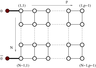
Figure 1: The $(\mathbb{CP}^{N-1})_{p}\times U(1)$ diagram.

This novel type of “crossed” Y-system, without shifts on the RHS , was first obtained in [19] and [20], in the context of the TBA for anomalous dimensions in the planar ${\cal N}=6$ superconformal Chern-Simons, i.e. $AdS_{4}/CFT_{3}$. Pictorially, the related $Y$-system diagram [19, 20] may be obtained from that for planar $AdS_{5}/CFT_{4}$ by means of some sort of ’folding’ process of the two wings with doubling of the fixed row of massive nodes; the same relation seems to hold (at strong coupling) between their low energy decoupled models, namely the present $\mathbb{CP}^{3}\times U(1)$ [9] and the $O(6)$ nonlinear sigma models [10], respectively. We shall give some details on this issue in Appendix B. At last but not least, an intriguing example of “crossed” $Y$-system describes the strong coupling behaviour of the gluon scattering amplitudes in $SYM_{4}$ [21].

Before concluding this section, we would like to make a final relevant generalisation. It is natural to consider a more general family of systems, stemming from the introduction of two positive integers $N$ and $p$, so that we conjecture for the massive nodes the equations

$$\begin{split}Y_{0}(\theta+i\frac{\pi}{2})\,\bar{Y}_{0}(\theta-i\frac{\pi}{2})&=\prod_{l=1}^{N-1}\left(1+Y_{(l,1)}(\theta+i\frac{\pi}{2}-i\frac{\pi l}{N})\right),\\ Y_{0}(\theta-i\frac{\pi}{2})\,\bar{Y}_{0}(\theta+i\frac{\pi}{2})&=\prod_{l=1}^{N-1}\left(1+Y_{(l,1)}(\theta-i\frac{\pi}{2}+i\frac{\pi l}{N})\right),\end{split}$$ (3.6)

while for the magnonic nodes the relations

$$Y_{(i,j)}(\theta+i\frac{\pi}{N})\,Y_{(i,j)}(\theta-i\frac{\pi}{N}) = \left(1+\delta_{i,1}\delta_{j,1}Y_{0}(\theta)+\delta_{i,N-1}\delta_{j,1}\bar{Y}_{0}(\theta)\right)\times$$ (3.7)

$$\times \prod_{l=1}^{p-1}\left(1+Y_{(i,l)}(\theta)\right)^{A_{l,j}^{(p-1)}}\prod_{l^{\prime}=1}^{N-1}\left(1+\displaystyle\frac{1}{Y_{(l^{\prime},j)}(\theta)}\right)^{-A_{l^{\prime},i}^{(N-1)}}\ \ ;$$

obviously, the system studied so far is recovered by fixing $(N,p)$ to $(4,\infty)$. With this simple generalisation, we are able to describe a previously-unknown infinite family of Y-systems naturally associated to a generic $SU(N)$ algebra with quantum reduced coset level $p$. As we shall see in the following section, the obtained truncated family of Y-systems exhibit all the important features common to more standard types of Y-systems. In particular, they can be interpreted as periodic sets of discrete recursion relations  [16] and their solutions lead to sum-rules [22] and functional identities for the Rogers dilogarithm [23] (See equation (5.1)).

Although the reader should keep in mind that most of the results presented in this paper have been rigorously derived only for $(N,p)=(4,\infty)$, from now on we shall leave the two positive integers $N$ and $p$ unconstrained. For later purpose, it is convenient to transform the Y-system into the Zamolodchikov’s universal TBA form [16]. Thanks to the Fourier integrals in (A.19), we obtain

$$\begin{split}\epsilon_{0}(\theta)&+\bar{\epsilon}_{0}(\theta)=2mR\cosh\theta-\sum_{l=1}^{N-1}\chi_{(1-\frac{2l}{N})}*\Lambda_{(l,1)}(\theta),\\ \epsilon_{0}(\theta)&-\bar{\epsilon}_{0}(\theta)=i2\alpha-\sum_{l=1}^{N-1}\psi_{(1-\frac{2l}{N})}*\Lambda_{(l,1)}(\theta),\\ \epsilon_{(i,j)}(\theta)&=\delta_{i,1}\delta_{j,1}\phi_{\frac{N}{2}}*L_{0}(\theta)+\delta_{i,N-1}\delta_{j,1}\phi_{\frac{N}{2}}*\bar{L}_{0}(\theta)+\sum_{l=1}^{p-1}A_{l,j}^{(p-1)}\phi_{\frac{N}{2}}*\Lambda_{(i,l)}(\theta)-\sum_{l=1}^{N-1}A_{l,i}^{(N-1)}\phi_{\frac{N}{2}}*L_{(l,j)}(\theta),\end{split}$$ (3.8)

with $\alpha\in\{0,\pi\}$, $\Lambda_{A}(\theta)=\ln(1+e^{\epsilon_{A}(\theta)})$ and the $\alpha$-vacuum energy given by equation (2.10) with

$$E_{\pm 1}(m,R)\simeq\mp\frac{2m}{\pi}C_{(N,p)}K_{1}(mR),$$ (3.9)

in the $Rm\gg 1$ infrared region. The coefficient $C_{(N,p)}$, which contains information on the $SU(N)$-related vacuum structure of the model at $(N,p)$ generic [24, 25], will be determined in the following Section.

4 The ultraviolet and infrared limits

The models under consideration can be thought of as 2d conformal field theories perturbed by a relevant operator which becomes marginally relevant in the limit $p\rightarrow\infty$ and whose vacuum energy is given by the expression (2.10) endowed with the groundstate TBA solution. In particular, the CFT is characterized by the value of its conformal anomaly, ${\bf c}_{(N,p)}$, which peculiarly enters the ($\alpha=0$) vacuum energy (2.10) in the $mR\ll 1$ ultraviolet regime [26]:

$$E_{+1}(m,R)\simeq-\frac{\pi{\bf c}_{(N,p)}}{6R}.$$ (4.1)

Thus, to obtain the central charge we have to study analytically the TBA equations in the limit $r=mR\rightarrow 0$. In this limit the solutions $\epsilon_{A}(\theta)$ to (3.8) develop a central plateau which broadens as $r$ approaches zero [5, 6]. The Casimir coefficient ${\bf c}_{(N,p)}$ acquires contributions from right and left kink-like regions, separately [5], and the result can be written as a sum-rule for the Rogers dilogarithm function

$$\mathcal{L}(x)=-\frac{1}{2}\int_{0}^{x}\left[\frac{\ln(1-t)}{t}+\frac{\ln t}{1-t}\right]dt,~{}~{}(0<x<1).$$ (4.2)

The final result is

$${\bf c}_{(N,p)}={\bf c}^{(0)}_{(N,p)}-{\bf c}^{(\infty)}_{(N,p)},$$ (4.3)

with

$${\bf c}^{(0)}_{(N,p)}=\frac{6}{\pi^{2}}\left[\mathcal{L}\left(\frac{y_{0}}{1+y_{0}}\right)+\mathcal{L}\left(\frac{\bar{y}_{0}}{1+\bar{y}_{0}}\right)+\sum_{i=1}^{N-1}\sum_{l=1}^{p-1}\mathcal{L}\left(\frac{y_{(i,l)}}{1+y_{(i,l)}}\right)\right],$$ (4.4)

and

$${\bf c}^{(\infty)}_{(N,p)}=\frac{6}{\pi^{2}}\sum_{i=1}^{N-1}\sum_{l=1}^{p-1}\mathcal{L}\left(\frac{z_{(i,l)}}{1+z_{(i,l)}}\right).$$ (4.5)

The constants $y$s are given by the $\theta$-independent (i.e. stationary) solutions of the Y-system, while the $z$s are the stationary solutions of (LABEL:YSS) with $Y_{0}=\bar{Y}_{0}=0$. The two relevant systems of stationary equations are

$$\begin{split}y_{0}\bar{y}_{0}&=\prod_{l^{\prime}=1}^{N-1}\left(1+y_{(l^{\prime},1)}\right),\\ (y_{(i,j)})^{2}&=\left(1+\delta_{i,1}\delta_{j,1}y_{0}+\delta_{i,N-1}\delta_{j,1}\bar{y}_{0}\right)\prod_{l=1}^{p-1}\left(1+y_{(i,l)}\right)^{A_{l,j}^{(p-1)}}\prod_{l^{\prime}=1}^{N-1}\left(1+\displaystyle\frac{1}{y_{(l^{\prime},j)}}\right)^{-A_{l^{\prime},i}^{(N-1)}},\end{split}$$ (4.6)

with $y_{0}=\bar{y}_{0}$ and $y_{(i,j)}=y_{(N-i,j)}$ ($i=1,\dots,N-1$, $j=1,2,\dots$), and

$$(z_{(i,j)})^{2}=\prod_{l=1}^{p-1}\left(1+z_{(i,l)}\right)^{A_{l,j}^{(p-1)}}\prod_{l^{\prime}=1}^{N-1}\left(1+\displaystyle\frac{1}{z_{(l^{\prime},j)}}\right)^{-A_{l^{\prime},i}^{(N-1)}}~{}.$$ (4.7)

Finding the exact solutions to equations (LABEL:YSS,4.6) for general $N>3$ and $p$ turned out to be much more difficult then expected. Setting $\varphi=\pi/(2(p+N-1))$, the results for lower ranks are the following

• $N=2$:

  $$y_{(1,i)}=(p-i)(p-i+2),~{}y_{0}=\bar{y}_{0}=p,$$ (4.8)

  with $i=1,2,\dots,p-1$.
  

• $N=3$:

  $$y_{(1,i)}=y_{(2,i)}=\frac{\sin((p-i)\varphi)\sin((p-i+3)\varphi)}{\sin(\varphi)\sin(2\varphi)},$$ (4.9)

  with $i=0,1,\dots,p-1$ and $y_{0}=\bar{y}_{0}=y_{(1,0)}=y_{(2,0)}$.
  

• $N=4$:

  $$y_{(1,p-1)}=y_{(3,p-1)}=\frac{2\sin(2\varphi)+\sin(6\varphi)+\sin(10\varphi)}{2\sin(6\varphi)},~{}y_{(2,p-1)}=\frac{2\sin(2\varphi)+\sin(6\varphi)+3\sin(10\varphi)}{2\sin(2\varphi)+3\sin(6\varphi)+\sin(10\varphi)}.$$ (4.10)

  (The stationary values for the remaining Y functions can be obtained using (LABEL:YSS) and (4.6) recursively.)

To deal with the generic $(N,p)$ case, we relied on a high-precision numerical work to conjecture the exact result for the dilogarithm sum-rule (4.4). Starting from $p=2$ and $N=2$ we were able to obtain the constants $y$s with a precision of about $10^{-15}$, for $p<20$ and $N<5$. The accuracy progressively decreased down to $10^{-12}$ for values around $p=61$ and $N=4$. The numerical results lead to the following precise conjecture

$${\bf c}_{(N,p)}^{(0)}=\frac{p(1+pN-p)}{p+N-1}.$$ (4.11)

The constant $z$s are instead analytically known to be [22]

$$z_{(i,j)}=\frac{\sin((j+N)\phi)\sin(j\phi)}{\sin((i+p)\phi)\sin(i\phi)},$$ (4.12)

with $\phi=\pi/(p+N)$, and the corresponding Rogers dilogarithm sum-rule is [22]

$${\bf c}_{(N,p)}^{(\infty)}=\frac{6}{\pi^{2}}\sum_{i=1}^{N-1}\sum_{l=1}^{p-1}\mathcal{L}\left(\frac{z_{(i,l)}}{1+z_{(i,l)}}\right)=\frac{p(N-1)(p-1)}{p+N}.$$ (4.13)

Finally, subtracting (4.13) from (4.11) we obtain

$${\bf c}_{(N,p)}=\frac{p(1-p-N+N^{2}+2Np)}{(N+p)(N+p-1)}=\frac{p\;\text{dim}[SU(N)]}{p+N}-\frac{p\;\text{dim}[SU(N-1)])}{p+N-1}$$ (4.14)

with $\text{dim}[SU(N)]=N^{2}-1$. The numerical outcome for the central charge at $N=4$ for the $p$-truncated models are compared with equation (4.14) in Table 1: the match is very good and leaves little doubt on the correctness of conjecture (4.11).

Level $p$	Numerics	Exact	Error
2	1.8000000000000014	9/5	$1.3\times 10^{-16}$
3	2.428571428571437	17/7	$8.4\times 10^{-15}$
4	2.928571428571431	41/14	$2.6\times 10^{-15}$
5	3.333333333333345	10/3	$6.7\times 10^{-15}$
6	3.666666666666656	11/3	$1.1\times 10^{-14}$
7	3.945454545454537	217/55	$8.4\times 10^{-15}$
8	4.181818181818161	46/11	$2.0\times 10^{-14}$
9	4.384615384615358	57/13	$2.7\times 10^{-14}$
10	4.56043956043953	415/91	$3.0\times 10^{-14}$
11	4.7142857142856	33/7	$1.1\times 10^{-13}$
41	6.212121212124	205/33	$2.8\times 10^{-12}$
51	6.35353535324	629/99	$2.9\times 10^{-10}$
61	6.4519230761	671/104	$8.2\times 10^{-10}$

Table 1: $N=4$: comparison between numerics and equation (4.14).

In conclusion, the central charge (4.14) deduced from equations (LABEL:YSS,3.6), coincides precisely with that of the coset model

$$(\mathbb{CP}^{N-1})_{p}\times U(1)=\frac{SU(N)_{p}}{SU(N-1)_{p}\times U(1)}\times U(1)\equiv\frac{SU(p)_{N-1}\times SU(p)_{1}}{SU(p)_{N}}\times U(1).$$ (4.15)

The Casimir coefficient for the $SU(N)\times U(1)$ sigma model is then recovered in the limit $p\rightarrow\infty$:

$${\bf c}_{(N,\infty)}=\text{dim}[SU(N)]-\text{dim}[SU(N-1)]=2N-1.$$ (4.16)

Thus ${\bf c}_{(4,\infty)}=7$, a result that coincides with the value predicted in [7] through a naive degree of freedom counting argument.

However, the identification of the model using only the Casimir coefficient is by no means unique as, for example, the two $U(1)$ factors in (4.15) yield compensating contributions to ${\bf c}_{(N,p)}$ leading to an equivalently good match with the central charge of the $\frac{SU(N)_{p}}{SU(N-1)_{p}}$ coset.

To further support the identification (4.15), following [16], we have determined the conformal dimension $\Delta_{(N,p)}$ of the perturbing operator using the intrinsic periodicity properties of the Y-system at finite $N$ and $p$.

Assuming arbitrary initial conditions and using the Y-system as a recursion relation, we descovered that the following periodicity property holds

$$Y_{A}\left(\theta+i\pi P_{(N,p)}\right)=Y_{A}(\theta),$$ (4.17)

with $P_{(N,p)}=\frac{2(p+N-1)}{N}$. Thus, according to [16] (cf. also [27, 17]), we can conclude that

$$\Delta_{(N,p)}=1-\frac{1}{P_{(N,p)}}=1-\frac{N}{2(p+N-1)},$$ (4.18)

is the conformal dimension of the operator which perturbs the conformal field theory at finite $p$ and generic $N$. A first consequence of (4.18), is that the model $\frac{SU(N)_{p}}{SU(N-1)_{p}}$ can be almost straightforwardly discarded. Furthermore, we have assumed that the two CFTs, originally disconnected and respectively related to $(\mathbb{CP}^{N-1})_{p}$ and $U(1)$, are tied together by the perturbing operator $\phi_{(N,p)}$ in the simplest possible way:

$$\phi_{(N,p)}=\phi_{[(\mathbb{CP}^{N-1})_{p}]}\times\phi_{[U(1)]},~{}~{}\Delta_{(N,p)}=\Delta_{[(\mathbb{CP}^{N-1})_{p}]}+\Delta_{[U(1)]}.$$ (4.19)

For the identification of $\Delta_{[(\mathbb{CP}^{N-1})_{p}]}$ and $\Delta_{[U(1)]}$, the presence of two independent integer parameters was very important as both $\Delta_{[(\mathbb{CP}^{N-1})_{p}]}$ and $\Delta_{[U(1)]}$ depend nontrivially on $N$ and $p$. At $p=1$, the TBA equations (3.8) reduce to those for a free fermion. This fact leads to

$$\Delta_{[(\mathbb{CP}^{N-1})_{1}]}=0~{},~{}~{}\Delta_{[U(1)]}=\Delta_{(N,1)}=1/2.$$ (4.20)

At $N=2$, the TBA equations coincide with the $D_{p+1}$ models with two massive nodes and a tail of magnons. These groun dstate TBA equations were identified in [28] (see, also [17]) –up to possible orbifold ambiguities– with a particular series of points of the fractional sine-Gordon model [29]. The latter identification leads to the further constant

$$\Delta_{[(\mathbb{CP}^{1})_{p}]}=\frac{(p-1)}{p}~{},~{}~{}\Delta_{[U(1)]}=\frac{1}{p(p+1)}.$$ (4.21)

Relations (4.20) and (4.21) together, allow to select the conformal dimension uniquely:

$$\Delta_{[(\mathbb{CP}^{N-1})_{p}]}=\frac{(p-1)(N+2p)}{2p(N+p-1)}~{},~{}~{}\Delta_{[U(1)]}=\frac{N}{2p(N+p-1)}.$$ (4.22)

It is interesting to notice that for $p=2$ the dimension $\Delta_{[(\mathbb{CP}^{N-1})_{p}]}$ corresponds to the field $\phi_{21}$ of the $c<1$ minimal models ${\cal M}_{N+1,N+2}$, while for generic $N$ and $p$ it coincides precisely with the conformal dimension of the field $(p,\bar{p},1)+(\bar{p},p,1)$ in the $W^{(p)}$ minimal model $\frac{SU(p)_{N-1}\times SU(p)_{1}}{SU(p)_{N}}$, mentioned by Fendley [30] while discussing integrability issues related to the purely-bosonic $\mathbb{CP}^{N-1}$ sigma model.

Finally, following [24, 25] equations (3.8) furnish in the infrared regime $mR\gg 1$

$$\epsilon_{0}(\theta)-i\alpha\simeq\bar{\epsilon}_{0}(\theta)+i\alpha\simeq mR\cosh\theta-\frac{1}{2}\sum_{l=1}^{N-1}\ln(1+z_{(l,1)}),$$ (4.23)

and consequently

$$E_{\pm 1}(m,R)\simeq\mp\frac{2m}{\pi}C_{(N,p)}K_{1}(mR),$$ (4.24)

with

$$C_{(N,p)}=\sqrt{\prod_{l=1}^{N-1}\left(1+z_{(l,1)}\right)}=\frac{\sin(N\phi)}{\sin(\phi)}\ ,$$ (4.25)

where we defined $\phi=\pi/(N+p)$. In the sigma model limit $p\rightarrow\infty$, then $\phi\rightarrow 0$ and (4.25) gives $C_{(N,\infty)}=N$, as expected.

5 Conclusions

In this paper we have proposed the Thermodynamic Bethe Ansatz equations and the Y-systems for an infinite family of perturbed conformal field theories related to the $\mathbb{CP}^{N-1}$ sigma models coupled to a massless Thirring fermion.

Although the main motivation of the work was the recently discovered description [9] of the low energy $AdS_{4}\times\mathbb{CP}^{3}$ string IIA sigma model ((strong) decoupling Alday-Maldacena limit [10]), most of the here derived results are of a much wider mathematical and physical interest. In particular, we have introduced a novel family of periodic Y-systems classified in terms of a pair of integers $(N,p)$. These functional relations differ from the standard Lie-algebra related ones, discussed for example in [16, 17, 18], in a non trivial way. In fact, not only the same $Y$-function appears in each LHS of the massive node equations (LABEL:YSS), but the massive $Y$s appear in a “crossed” way (cf. also Appendix B for some considerations).

Many important features of Y-systems were recently investigated and proved by means of very powerful Cluster Algebra methods (see, for example the review [31]). Within the latter mathematical setup, it would be important to clarify whether the Y-systems introduced here are genuinely new objects or otherwise they lead to Cluster Algebra quivers that are mutation-equivalent to some of the known ABCD-related cases [31] (cf., for example, the discussion in Section 7.3 of [34]).

Some of the mathematical results presented here correspond to numerical-supported conjectures and, although we have little doubt on their exact validity, it would be still important to prove them rigorously.

The main mathematical conjectures are: the Y-system periodicity (4.17), the stationary dilogarithm identities (4.11) and the following non stationary sum-rules

$$\sum_{n=1}^{2(N+p-1)}\left(\mathcal{L}\left(\frac{\bar{Y}_{0}(n)}{1+\bar{Y}_{0}(n)}\right)+\mathcal{L}\left(\frac{Y_{0}(n)}{1+Y_{0}(n)}\right)+\sum_{i=1}^{N-1}\sum_{j=1}^{p-1}\mathcal{L}\left(\frac{Y_{(i,j)}(n)}{1+Y_{(i,j)}(n)}\right)\right)=2p(1+pN-p)\frac{\pi^{2}}{6},$$ (5.1)

where $Y_{A}(n)=Y_{A}\left(\theta+i\frac{\pi}{N}n\right)$ are the solutions of the Y-system, obtained recursively from (LABEL:YSS, 3.6) with arbitrary initial conditions [23].

Concerning the specific $\mathbb{CP}^{3}\times U(1)$ sigma model, we have performed a non-trivial computation of the ultraviolet central charge from TBA/$Y$-system, confirming the results predicted in [7] through a naive counting of the degrees of freedom. In fact, our conclusions were reached using highly non trivial dilogarithm identities and by considering the sigma model as the $p\rightarrow\infty$ representative in the family of perturbed coset conformal field theories $\frac{SU(4)_{p}}{SU(3)_{p}\times U(1)}\times U(1)$, and concerned also the perturbing field.

Apart from the physical and mathematical aspects mentioned above, there are many other issues that we would like to address in the near future: the kink vacuum structure, the exact S-matrix and the mass-coupling relation for the quantum truncated models, the numerical study of the TBA equations for the excited states [35] and the derivation of simpler non-linear integral equations for both the groundstate and the excited states [36] are only a small sample of important open problems that deserve further attention.

Acknowledgments– We thank Diego Bombardelli, Andrea Cavaglià, Francesco Ravanini, Marco Rossi and Gerard Watts for useful discussions and help. SP and AF are grateful respectively to the Centro de Física do Porto and to IPhT-Saclay for kind hospitality. This project was partially supported by INFN grants IS FI11, P14, PI11, the Italian MIUR-PRIN contract 2009KHZKRX-007 “Symmetries of the Universe and of the Fundamental Interactions”, the UniTo-SanPaolo research grant Nr TO-Call3-2012-0088 “Modern Applications of String Theory” (MAST), the ESF Network “Holographic methods for strongly coupled systems” (HoloGrav) (09-RNP-092 (PESC)) and MPNS–COST Action MP1210 “The String Theory Universe”.

Appendix A Scattering amplitudes and TBA kernels

This appendix contains the explicit expressions for scattering amplitudes and the corresponding TBA kernels used throughout the main text.

Spinon-Spinon scattering

The spinon-spinon $S$-matrix amplitude [7] is

$$S(\theta)=-\frac{\displaystyle\Gamma\left(1+i\frac{\theta}{2\pi}\right)\Gamma\left(\frac{1}{4}-i\frac{\theta}{2\pi}\right)}{\displaystyle\Gamma\left(1-i\frac{\theta}{2\pi}\right)\Gamma\left(\frac{1}{4}+i\frac{\theta}{2\pi}\right)},$$ (A.1)

and the corresponding kernel $\mathcal{K}(\theta)$

$$\mathcal{K}(\theta)=\frac{1}{2\pi i}\frac{\partial}{\partial\theta}\ln S(\theta),$$ (A.2)

which may be represented in several alternative ways as

$$\begin{split}\mathcal{K}(\theta)&=\frac{1}{4\pi^{2}}\left(\psi\left(1+i\frac{\theta}{2\pi}\right)+\psi\left(1-i\frac{\theta}{2\pi}\right)-\psi\left(\frac{1}{4}+i\frac{\theta}{2\pi}\right)-\psi\left(\frac{1}{4}-i\frac{\theta}{2\pi}\right)\right)\\ &=\sum_{n=0}^{\infty}\left(\frac{1}{\pi}\frac{2\pi(n+1/4)}{\theta^{2}+(2\pi(n+1/4))^{2}}-\frac{1}{\pi}\frac{2\pi(n+1)}{\theta^{2}+(2\pi(n+1))^{2}}\right)\\ &=\int_{-\infty}^{\infty}\frac{d\omega}{2\pi}e^{i\omega\theta}\,\frac{q-q^{4}}{1-q^{4}},\end{split}$$ (A.4)

with $q=\exp\left(-\frac{\pi}{2}|\omega|\right)$. It is straightforward to get

$$\int_{-\infty}^{\infty}d\theta\,\mathcal{K}(\theta)=\lim_{\omega\rightarrow 0}\hat{\mathcal{K}}(\omega)=\frac{3}{4}.$$ (A.5)

Spinon-antispinon scattering

The $S$-matrix amplitude associated to the spinon-antispinon scattering is

$$t_{1}(\theta)=\frac{\displaystyle\Gamma\left(\frac{1}{2}-i\frac{\theta}{2\pi}\right)\Gamma\left(\frac{3}{4}+i\frac{\theta}{2\pi}\right)}{\displaystyle\Gamma\left(\frac{1}{2}+i\frac{\theta}{2\pi}\right)\Gamma\left(\frac{3}{4}-i\frac{\theta}{2\pi}\right)}.$$ (A.6)

Consequently the kernel $G(\theta)$ is

$$G(\theta)=\frac{1}{2\pi i}\frac{\partial}{\partial\theta}\ln t_{1}(\theta),$$ (A.7)

explicitly

$$\begin{split}G(\theta)&=\frac{1}{4\pi^{2}}\left(\psi\left(\frac{3}{4}+i\frac{\theta}{2\pi}\right)+\psi\left(\frac{3}{4}-i\frac{\theta}{2\pi}\right)-\psi\left(\frac{1}{2}+i\frac{\theta}{2\pi}\right)-\psi\left(\frac{1}{2}-i\frac{\theta}{2\pi}\right)\right)\\ &=\sum_{n=0}^{\infty}\left(\frac{1}{\pi}\frac{2\pi(n+1/2)}{\theta^{2}+(2\pi(n+1/2))^{2}}-\frac{1}{\pi}\frac{2\pi(n+3/4)}{\theta^{2}+(2\pi(n+3/4))^{2}}\right)\\ &=\int_{-\infty}^{\infty}\frac{d\omega}{2\pi}e^{i\omega\theta}\,\frac{q^{2}-q^{3}}{1-q^{4}},\end{split}$$ (A.8)

with $q=\exp\left(-\frac{\pi}{2}|\omega|\right)$. Then

$$\int_{-\infty}^{\infty}d\theta\,G(\theta)=\lim_{\omega\rightarrow 0}\hat{G}(\omega)=\frac{1}{4}.$$ (A.9)

Magnon bound state scattering

Magnonic string solutions scatter according to the amplitudes

$$S_{l,m}(\theta)=\prod_{a=\frac{|l-m|+1}{2}}^{\frac{l+m-1}{2}}\left(\frac{\displaystyle\theta-i\frac{\pi a}{2}}{\displaystyle\theta+i\frac{\pi a}{2}}\right),$$ (A.10)

from which

$$K_{l,m}(\theta)=\frac{1}{2\pi i}\frac{\partial}{\partial\theta}\ln S_{lm}(\theta)=\sum_{a=\frac{|l-m|+1}{2}}^{\frac{l+m-1}{2}}\frac{1}{\pi}\frac{a\pi/2}{\theta^{2}+(a\pi/2)^{2}}.$$ (A.11)

Fourier transforming (A.11) gives

$$\hat{K}_{l,m}(\omega)=\sum_{a=\frac{|l-m|+1}{2}}^{\frac{l+m-1}{2}}e^{-a|\omega|\pi/2}=\frac{e^{-\frac{|\omega|\pi}{4}|l-m|}-e^{-\frac{|\omega|\pi}{4}(l+m)}}{2\sinh(\pi|\omega|/4)},$$ (A.12)

and the matrix

$$N_{l,m}=\int_{-\infty}^{\infty}d\theta K_{l,m}(\theta)=\hat{K}_{l,m}(0)=\min[l,m]=\frac{l+m-|l-m|}{2},$$ (A.13)

whose inverse is

$$\hat{K}_{n,l}^{-1}(\omega)=2\cosh\left(\frac{|\omega|\pi}{4}\right)\delta_{nl}-\left(\delta_{n,l-1}+\delta_{n,l+1}\right),$$ (A.14)

with

$$\sum_{l}\hat{K}_{n,l}^{-1}(\omega)\hat{K}_{l,m}(\omega)=\delta_{n,m}.$$ (A.15)

Helpful Relations in Bootstrapping Matrices and Kernels

Here we are reviewing the identities between scattering matrices (cfr [16][17]) required in order to write down the $Y$-system and universal form TBA

$$\begin{split}&S_{lm}\left(\theta+\frac{i\pi}{4}\right)\,S_{lm}\left(\theta-\frac{i\pi}{4}\right)=S_{l-1,m}\left(\theta\right)\,S_{l+1,m}\left(\theta\right)\,e^{2\pi i\Theta(\theta)\,\delta_{lm}}\\ &t_{1}\left(\theta+\frac{i\pi}{4}\right)\,t_{1}\left(\theta-\frac{i\pi}{4}\right)=-S\left(\theta+\frac{i\pi}{4}\right)\,S\left(\theta-\frac{i\pi}{4}\right)\,[S_{11}(\theta)]^{-1}\\ &S\left(\theta+\frac{i\pi}{2}\right)\,S\left(\theta-\frac{i\pi}{2}\right)=-\frac{t_{1}(\theta)}{S(\theta)}S_{12}(\theta)\,e^{2\pi i\Theta(\theta)}\\ &t_{1}\left(\theta+\frac{i\pi}{2}\right)\,t_{1}\left(\theta-\frac{i\pi}{2}\right)=-\frac{S(\theta)}{t_{1}(\theta)}\\ &S_{lm}\left(\theta+\frac{i\pi}{2}\right)\,S_{lm}\left(\theta-\frac{i\pi}{2}\right)=S_{l-2,m}\left(\theta\right)\,S_{l+2,m}\left(\theta\right)\,e^{2\pi i\Theta(\theta)\,I_{lm}}\end{split}$$ (A.16)

($\Theta(x)$ stands for the Heaviside step function, while $I_{lm}=\delta_{l-1,m}+\delta_{l+1,m}$ ). These relations are reflected into the following ones, involving the kernels:

$$\begin{split}&K_{lm}\left(\theta+\frac{i\pi}{4}\right)+K_{lm}\left(\theta-\frac{i\pi}{4}\right)=K_{l-1,m}\left(\theta\right)+K_{l+1,m}\left(\theta\right)+\delta(\theta)\,\delta_{lm}\\ &G\left(\theta+\frac{i\pi}{4}\right)+G\left(\theta-\frac{i\pi}{4}\right)=\mathcal{K}\left(\theta+\frac{i\pi}{4}\right)+\mathcal{K}\left(\theta-\frac{i\pi}{4}\right)-K_{11}(\theta)\\ &\mathcal{K}\left(\theta+\frac{i\pi}{2}\right)+\mathcal{K}\left(\theta-\frac{i\pi}{2}\right)=-\mathcal{K}(\theta)+G(\theta)+K_{12}(\theta)+\delta(\theta)\\ &G\left(\theta+\frac{i\pi}{2}\right)+G\left(\theta-\frac{i\pi}{2}\right)=\mathcal{K}(\theta)-G(\theta)\\ &K_{lm}\left(\theta+\frac{i\pi}{2}\right)+K_{lm}\left(\theta-\frac{i\pi}{2}\right)=K_{l-2,m}\left(\theta\right)+K_{l+2,m}\left(\theta\right)+\delta(\theta)\,I_{lm}+\\ &\qquad\qquad+\delta_{l1}\,\delta_{m1}\left[\delta(\theta+\frac{i\pi}{4})+\delta(\theta-\frac{i\pi}{4})\right]\end{split}$$ (A.17)

(the last relation makes sense provided we define $K_{l,0}=0\ ,\ K_{l,-1}=-K_{l,1}$). Moreover, we find:

$$\begin{split}&\mathcal{K}(\theta+\frac{i\pi}{2})+G(\theta-\frac{i\pi}{2})-K_{11}(\theta+\frac{i\pi}{4})\,=\,0\\ &\mathcal{K}(\theta-\frac{i\pi}{2})+G(\theta+\frac{i\pi}{2})-K_{11}(\theta-\frac{i\pi}{4})\,=\,0\\ &\mathcal{K}(\theta+\frac{i\pi}{2})+G(\theta-\frac{i\pi}{2})+K_{11}(\theta-\frac{i\pi}{4})\,=\,K_{12}(\theta)+\delta(\theta)\\ &\mathcal{K}(\theta-\frac{i\pi}{2})+G(\theta+\frac{i\pi}{2})+K_{11}(\theta+\frac{i\pi}{4})\,=\,K_{12}(\theta)+\delta(\theta)\end{split}$$ (A.18)

The universal kernels

The kernels appearing in the Zamolodchikov’s universal form of the TBA equations (3.8) are

$$\begin{split}\int_{-\infty}^{\infty}\frac{d\omega}{2\pi}\frac{\cosh(\frac{\pi}{2}a\omega)}{\cosh(\frac{\pi\omega}{2})}\,e^{i\omega\theta}&=\frac{2}{\pi}\frac{\cos(a\pi/2)\cosh\theta}{\cos(a\pi)+\cosh(2\theta)}=\chi_{a}(\theta),\\ \int_{-\infty}^{\infty}\frac{d\omega}{2\pi}\frac{\sinh(\frac{\pi}{2}a\omega)}{\sinh(\frac{\pi\omega}{2})}\,e^{i\omega\theta}&=\frac{1}{\pi}\frac{\sin(a\pi)}{\cos(a\pi)+\cosh(2\theta)}=\psi_{a}(\theta),\\ \int_{-\infty}^{\infty}\frac{d\omega}{2\pi}\frac{1}{2\cosh(\frac{\pi\omega}{2a})}\,e^{i\omega\theta}&=\frac{a}{2\pi\,\cosh(a\theta)}=\phi_{a}(\theta).\end{split}$$ (A.19)

Appendix B Folding diagrams

We wish now to discuss some features about a pictorial folding process of diagrams, by elucidating an inspiring resemblance between the $Y$-system diagrams for the $O(6)$ Non-Linear Sigma Model and the $\mathbb{CP}^{3}\times U(1)$ model considered throughout this paper.

The $O(2n)$ Non-Linear Sigma Model TBA and Y-system
According to [30, 32, 33] we can write the TBA system for the $O(2n)$ ($n\geq 2$) Non-Linear Sigma Models as the limit of a certain sequence of coupled non-linear integral equations which read

$$\begin{split}&\epsilon_{0}(\theta)=mR\cosh\theta-\sum_{j=1}^{n-2}\chi_{\frac{2}{g}(n-1-j)}\ast L_{(j,1)}(\theta)-\phi_{1}\ast[L_{(n-1,1)}+L_{(n,1)}]\end{split}$$ (B.1)

$$\begin{split}\epsilon_{(a,m)}(\theta)=-\delta_{m1}[\delta_{a1}+\delta_{a2}\delta_{n2}]\,\phi_{\frac{g}{2}}\ast L_{0}(\theta)-\,\phi_{\frac{g}{2}}\ast[L_{(a,m-1)}+L_{(a,m+1)}]+\sum_{b=1}^{n}\,I_{ab}\,\phi_{\frac{g}{2}}\ast\Lambda_{(b,m)}(\theta)\end{split}$$ (B.2)

where $g=2(n-1)$ and $I_{ab}$ are respectively the Coxeter number and the incidence matrix associated to the $D_{n}$ Lie algebra, while we defined

$$L_{0}(\theta)=\ln\left(1+e^{-\epsilon_{0}(\theta)}\right)\qquad L_{(a,m)}(\theta)=\ln\left(1+e^{-\epsilon_{(a,m)}(\theta)}\right)\qquad\Lambda_{(a,m)}(\theta)=\ln\left(1+e^{\epsilon_{(a,m)}(\theta)}\right)\ \ .$$ (B.3)

By means of the kernel relation

$$\chi_{\frac{2}{g}(n-1-j)}(\theta+\frac{i\pi}{2})\,+\,\chi_{\frac{2}{g}(n-1-j)}(\theta-\frac{i\pi}{2})=\delta(\theta+\frac{i(n-1-j)\pi}{g})+\delta(\theta-\frac{i(n-1-j)\pi}{g})\,\,\,,$$ (B.4)

and upon defining (as usual)

$$\begin{split}&X_{(a\,,m)}(\theta)=e^{-\epsilon_{(a,m)}(\theta)}\\ &X_{0}(\theta)=e^{-\epsilon_{0}(\theta)}\qquad,\end{split}$$ (B.5)

equation (B.1) entails

$$\begin{split}\epsilon_{0}\left(\theta+\frac{i\pi}{2}\right)+&\epsilon_{0}\left(\theta-\frac{i\pi}{2}\right)=-\sum_{a=1}^{n-2}\left[\ln\left(1+X_{(a,1)}(\theta-\frac{i(n-1-a)\pi}{g})\right)\right.+\\ +&\left.\ln\left(1+X_{(a,1)}(\theta+\frac{i(n-1-a)\pi}{g})\right)\right]-\ln\left(1+X_{(n-1,1)}(\theta)\right)-\ln\left(1+X_{(n,1)}(\theta)\right)\qquad.\end{split}$$ (B.6)

The latter is the first functional equation of the full $Y$-system

$$\begin{split}X_{0}\left(\theta+\frac{i\pi}{2}\right)&X_{0}\left(\theta-\frac{i\pi}{2}\right)=\prod_{a=1}^{n-2}\left[\left(1+X_{(a,1)}(\theta-\frac{i(n-1-a)\pi}{g})\right)\right.\times\\ &\times\left.\left(1+X_{(a,\,1)}(\theta+\frac{i(n-1-a)\pi}{g})\right)\right]\left(1+X_{(n-1,\,1)}(\theta)\right)\left(1+X_{(n,\,1)}(\theta)\right)\\ X_{(a,m)}\left(\theta+\frac{i\pi}{g}\right)&X_{(a,m)}\left(\theta-\frac{i\pi}{g}\right)=[1+\delta_{1m}(\delta_{a1}+\delta_{n2}\delta_{a2})X_{0}(\theta)]\frac{(1+X_{(a,m+1)}(\theta))(1+X_{(a,m-1)}(\theta))}{\displaystyle\prod_{b=1}^{n}\left(1+\frac{1}{X_{(b,m)}(\theta)}\right)^{I_{ab}}}\,\,\,,\end{split}$$ (B.7)

which may be encoded in the diagram of Fig.(2) . The bold link has the same meaning (explained in footnote 2 on page 6) as in the $\mathbb{CP}^{N-1}\times U(1)$ model diagram of Fig.(1).

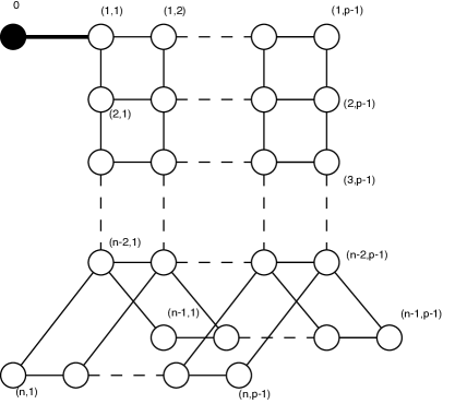
Figure 2: The $O(2n)$ diagram. The labels of each node are associated to the functions $Y$ in (B.7)

Folding diagrams
In the particular case $n=3$, the $Y$-system of the $O(6)$ non-linear sigma model reads

$$\begin{split}X_{0}(\theta+\frac{i\pi}{2})X_{0}(\theta-\frac{i\pi}{2})=\left(1+X_{(2,1)}(\theta+\frac{i\pi}{4})\right)\left(1+X_{(2,1)}(\theta-\frac{i\pi}{4})\right)\left(1+X_{(1,1)}\right)\left(1+X_{(3,1)}\right)\\ \end{split}$$

$$X_{(a,m)}(\theta+\frac{i\pi}{4})X_{(a,m)}(\theta-\frac{i\pi}{4})=\left(1+\delta_{m1}\delta_{a2}X_{0}\right)\frac{\left(1+X_{(a,m+1)}\right)\left(1+X_{(a,m-1)}\right)}{\left(1+\displaystyle\frac{1}{X_{(a+1,m)}}\right)\left(1+\displaystyle\frac{1}{X_{(a-1,m)}}\right)}\qquad\begin{array}[]{ccc}&a=1,2,3\\ &m=1,2,3,...,p-1\end{array}$$ (B.8)

(imposing $X_{(a,0)}=X_{(a,p)}=(X_{(0,m)})^{-1}=(X_{(4,m)})^{-1}=0$ and taking the limit $p\rightarrow\infty$), which may be represented on the diagram in Fig.(3) and enjoys the usual (uncrossed) form.

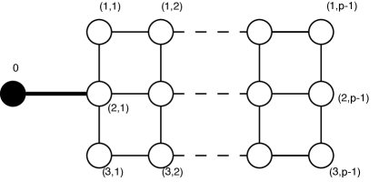
Figure 3: The $O(6)$ diagram. The labels of each node are to be intended as the subscripts of the functions $X$ appearing in (B.8).

Moving from this $O(6)$ diagram we may think to construct that of Fig.(1) for $N=4,p=\infty$ paralleling the graphic folding procedure resulting in the $AdS_{4}$ digram [19] from that of $AdS_{5}$, as described previously in the main text. Namely, we can merge together rows $1$ and $3$ in Fig.(3), while all nodes along the symmetry row $2$ (including the massive node) shall split into two nodes. In particular, the unique massive node $0$ is ’torn’ into two, that is, we can imagine, the spinon $0$ and the antispinon $\bar{0}$ in Fig.(1) (for $N=4$). The latter need now to satisfy the ’crossed’ equations (3.5).

The physical and mathematical implications of this observation are left for ongoing investigations, also in relation to other folding [37] and quiver [31, 34] procedures.

References

[1]
J.M. Maldacena,
The large limit of superconformal field theories and supergravity,
Adv. Theor. Math. Phys. 2, 231 (1998), [arXiv:hep-th/9711200].
[2]
E. Witten,
Anti-de Sitter space and holography,
Adv. Theor. Math. Phys. 2, 253 (1998), [arXiv:hep-th/9802150].
[3]
L.N. Lipatov,
Asymptotic behavior of multicolor QCD at high energies in connection with exactly solvable spin models,
JETP Lett. 59, 596 (1994),
[Pisma Zh. Eksp. Teor. Fiz.59, 571 (1994)]. L.D. Faddeev and G.P. Korchemsky,
High-energy QCD as a completely integrable model,
Phys. Lett. B342, 311 (1995),
[arXiv:hep-th/9404173].
[4]
J.A. Minahan and K. Zarembo,
The Bethe Ansatz for
Super Yang-Mills, JHEP03, 013 (2003), [arXiv:hep-th/0212208]. N. Beisert and M. Staudacher,
Long-range Bethe Ansatz for gauge theory and strings,
Nucl. Phys. B727,1 (2005),
[arXiv:hep-th/0504190]. J.A. Minahan and K. Zarembo,
The Bethe Ansatz for superconformal Chern-Simons,
JHEP0809, 040 (2008),
[arXiv:0806.3951 [hep-th]]. N. Beisert and M. Staudacher,
Long-range psu(2,24) Bethe Ansätze for gauge theory and strings,
Nucl. Phys. B727, 1 (2005),
[arXiv:hep-th/0504190]. N. Gromov and P. Vieira,
The all loop Bethe Ansatz,
JHEP0901, 016 (2009),
[arXiv:0807.0777 [hep-th]]. C. Ahn and R.I. Nepomechie,
N=6 super Chern-Simons theory S-matrix and all-loop Bethe Ansatz equations,
JHEP0809, 010 (2008),
[arXiv:0807.1924 [hep-th]]. N. Gromov, V. Kazakov and P. Vieira,
Exact spectrum of anomalous dimensions of planar N=4 Supersymmetric Yang-Mills theory,
Phys. Rev. Lett. 103, 131601 (2009),
[arXiv:0901.3753 [hep-th]] (arXiv title:Integrability for the full spectrum of planar AdS/CFT). D. Bombardelli, D. Fioravanti and R. Tateo,
Thermodynamic Bethe Ansatz for planar AdS/CFT: a proposal,
J. Phys. A42, 375401 (2009),
[arXiv:0902.3930 [hep-th]]. N. Gromov, V. Kazakov, A. Kozak and P. Vieira,
Integrability for the full spectrum of planar AdS/CFT II,
[arXiv:0902.4458 [hep-th]]. G. Arutyunov and S. Frolov,
Thermodynamic Bethe Ansatz for the Mirror Model,
JHEP0905, 068 (2009),
[arXiv:0903.0141 [hep-th]].
[5]
Al.B. Zamolodchikov,
Thermodynamic Bethe Ansatz in relativistic models: Scaling 3-state Potts and Lee-Yang models,
Nucl. Phys. B338, 485 (1990).
[6]
T. Klassen and E. Melzer,
Purely elastic scattering theories and their ultraviolet limits,
Nucl. Phys B342, 695 (1990). T. Klassen and E. Melzer,
The thermodynamics of purely elastic scattering theories and conformal perturbation theory,
Nucl. Phys. B350, 635 (1991).
[7]
B. Basso and A. Rej,
On the integrability of two-dimensional models with symmetry,
Nucl. Phys. B866, 337 (2013), [arXiv:1207.0413 [hep-th]].
[8]
E. Witten,
Instantons, the Quark Model, and the 1/n Expansion,
Nucl. Phys. B149, 285 (1979).
[9]
D. Bykov,
The worldsheet low-energy limit of the superstring,
Nucl. Phys. B838, 47 (2010),
[arXiv:1003.2199 [hep-th]].
[10]
L.F. Alday and J.M. Maldacena,
Comments on operators with large spin,
JHEP0711, 019 (2007),
[arXiv:0708.0672 [hep-th]]. D. Fioravanti, P. Grinza and M. Rossi,
Strong coupling for planar SYM theory: an all-order result,
Nucl.Phys. B810 (2009) 563-574,
[arXiv:0804.2893 [hep-th]]. B. Basso and G.P. Korchemsky,
Embedding nonlinear sigma model into super-Yang-Mills theory,
Nucl.Phys. B807 (2009) 397-423,
[arXiv:0805.4194 [hep-th]]. D. Fioravanti, P. Grinza and M. Rossi,
The generalized scaling function: a note,
Nucl.Phys. B827 (2010) 359-380,
[arXiv:0805.4407 [hep-th]]. D. Fioravanti, P. Grinza and M. Rossi,
Generalized scaling function: a systematic study,
JHEP0911 (2009) 037,
[arXiv:0808.1886 [hep-th]].
[11]
B. Basso and A. Rej,
Bethe Ansaetze for GKP strings,
[arXiv:1306.1741 [hep-th]].
[12]
M. Takahashi and M. Suzuki,
One-dimensional anisotropic Heisenberg model at finite temperatures,
Prog. Theor. Phys. 48, 2187 (1972).
[13]
M.J. Martins,
Complex excitations in the thermodynamic Bethe ansatz approach,
Phys. Rev. Lett. 67, 419 (1991).
[14]
P. Fendley,
Excited state thermodynamics,
Nucl. Phys. B374, 667 (1992),
[hep-th/9109021].
[15]
V. Privman and M.E. Fisher,
Finite-size effects at first-order transitions,
J. Stat. Phys. 33, 385 (1983). E. Brézin and J. Zinn-Justin,
Finite size effects in phase transitions,
Nucl. Phys. B257, 867 (1985). G. Münster,
Tunneling amplitude and surface tension in -theory,
Nucl. Phys.B324, 630 (1989). K. Jansen and Y. Shen,
Tunneling and energy splitting in Ising models,
Nucl. Phys. B393, 658 (1993).
[16]
Al.B. Zamolodchikov,
On the Thermodynamic Bethe equations for reflectionless ADE scattering theories,
Phys. Lett. B253, 391 (1991).
[17]
F. Ravanini, R. Tateo and A. Valleriani,
Dynkin TBA’s,
Int. J. Mod. Phys. A8, 1707 (1993), [arXiv:hep-th/9207040].
[18]
A. Kuniba, T. Nakanishi and J. Suzuki,
Functional relations in solvable lattice models. 1:
Functional relations and representation theory,
Int. J. Mod. Phys. A9, 5215 (1994),
[hep-th/9309137].
[19]
D. Bombardelli, D. Fioravanti and R. Tateo,
TBA and Y-system for planar ,
Nucl. Phys. B834, 543 (2010), [arXiv:0912.4715 [hep-th]].
[20]
N. Gromov and F. Levkovich-Maslyuk,
Y-system, TBA and quasi-classical strings in ,
JHEP1006, 088 (2010),
[arXiv:0912.4911 [hep-th]].
[21]
L.F. Alday, J. Maldacena, A. Sever and P. Vieira,
Y-system for scattering amplitudes,
J. Phys. A43, 485401 (2010), [arXiv:1002.2459 [hep-th]].
[25]
P. Dorey, R. Tateo and K.E. Thompson,
Massive and massless phases in selfdual Z(N) spin models: Some exact results from the thermodynamic Bethe ansatz,
Nucl. Phys. B470, 317 (1996),[hep-th/9601123].
[26]
H. Bloete, J.L. Cardy and M. Nightingale,
Confromal invariance, the central charge, and universal finite size amplitudes at criticality,
Phys. Rev. Lett. 56, 742 (1986).
[28]
R. Tateo,
The sine-Gordon model as -perturbed coset
theory and generalizations,
Int. J. Mod. Phys. A10, 1357 (1995),
[hep-th/9405197].
[29]
D. Bernard and A. Leclair,
The fractional supersymmetric sine-Gordon models,
Phys. Lett. B247, 309 (1990).
[30]
P. Fendley,
Sigma models as perturbed conformal field theories,
Phys. Rev. Lett. 83, 4468 (1999), [arXiv:hep-th/9906036]. P. Fendley,
Integrable sigma models and perturbed coset models,
JHEP0105, 050 (2001), [arXiv:hep-th/0101034].
[31]
A. Kuniba, T. Nakanishi and J. Suzuki,
T-systems and Y-systems in integrable systems,
J. Phys. A44, 103001 (2011),
[arXiv:1010.1344 [hep-th]].
[32]
J. Balog and A. Hegedus,
Virial expansion and TBA in O(N) sigma models,
Phys. Lett. B523 (2001) 211
[hep-th/0108071].
[33]
J. Balog and A. Hegedus,
TBA equations for the mass gap in the O(2r) non-linear sigma-models,
Nucl. Phys. B725 (2005) 531
[hep-th/0504186].
[34]
T. Nakanishi and R. Tateo,
Dilogarithm identities for sine-Gordon and reduced sine-Gordon Y-systems,
SIGMA 6, 085 (2010),[arXiv:1005.4199 [math.QA]].
[35]
V.V. Bazhanov, S.L. Lukyanov and A.B. Zamolodchikov,
Integrable quantum field theories in finite volume: Excited state energies,
Nucl. Phys. B489, 487 (1997)
[hep-th/9607099]. P. Dorey and R.Tateo,
Excited states by analytic continuation of TBA equations,
Nucl. Phys. B482, 639 (1996),
[hep-th/9607167]. P. Dorey and R. Tateo,
Excited states in some simple perturbed conformal field theories,
Nucl. Phys. B515, 575 (1998)
[hep-th/9706140].
[36]
A. Klumper, M.T. Batchelor and P.A. Pearce,
Central charges of the 6- and 19- vertex models with twisted boundary conditions,
J. Phys. A24, 3111 (1991). C. Destri and H.J. de Vega,
New thermodynamic Bethe ansatz equations without strings,
Phys. Rev. Lett. 69, 2313 (1992). D. Fioravanti, A. Mariottini, E. Quattrini and F. Ravanini,
Excited state Destri-De Vega equation for sine-Gordon and restricted sine-Gordon models,
Phys. Lett. B390, 243 (1997), [hep-th/9608091]. G. Feverati, F. Ravanini and G.Takacs,
Nonlinear integral equation and finite volume spectrum of sine-Gordon theory,
Nucl. Phys. B540, 543 (1999), [hep-th/9805117]. D. Bombardelli, D. Fioravanti and M. Rossi,
Large spin corrections in N = 4 SYM sl(2): Still a linear integral equation,
Nucl. Phys. B810, 460 (2009)
[arXiv:0802.0027 [hep-th]]. N. Gromov, V. Kazakov, S. Leurent and D. Volin,
Solving the AdS/CFT Y-system,
JHEP1207, 023 (2012),
[arXiv:1110.0562 [hep-th]]. J. Balog and A. Hegedus,
Hybrid-NLIE for the AdS/CFT spectral problem,
JHEP1208, 022 (2012),
[arXiv:1202.3244 [hep-th]]. D. Fioravanti, S. Piscaglia and M. Rossi,
On the scattering over the GKP vacuum,
[arXiv:1306.2292 [hep-th]].
[37]
P. Fendley and P. H. Ginsparg,
Noncritical orbifolds,
Nucl. Phys. B324, 549 (1989).