Poisson’s equation for discrete-time quasi-birth-and-death processes

Abstract

We consider Poisson’s equation for quasi-birth-and-death processes (QBDs) and we exploit the special transition structure of QBDs to obtain its solutions in two different forms. One is based on a decomposition through first passage times to lower levels, the other is based on a recursive expression for the deviation matrix.

We revisit the link between a solution of Poisson’s equation and perturbation analysis and we show that it applies to QBDs. We conclude with the PH/M/1 queue as an illustrative example, and we measure the sensitivity of the expected queue size to the initial value.

Keywords: Quasi-birth-and-death process, Poisson’s equation, perturbation analysis, matrix-analytic method.

1 Introduction

Poisson’s equation has the following form:

$$(I-P){{\boldsymbol{h}}}={{\boldsymbol{g}}},$$ (1)

where $P$ is the transition matrix of a Markov chain on some denumerable state space $\mathbb{E}$ and ${\boldsymbol{g}}$ is a given vector on $\mathbb{E}$, subject to some constraints. Equations of the form (1) frequently occur in the analysis of Markov chains. In particular, as remarked in Meyn and Tweedie [21, Pages 458-459], we find them in the context of central limit theorems, perturbation theory, controlled Markov processes, variance analysis of simulation algorithms, etc. It is of interest to note that the equation has been analyzed in cases where the state space is continuous: Glynn [9] derives a solution of Poisson’s equation for the waiting time process of the recurrent discrete-time M/G/1 queue, and Asmussen and Bladt [2] consider the waiting time for continuous-time queues driven by a Markovian marked point process.

Here, we assume that the Markov chain is a quasi-birth-and-death process (QBD): the state space is $\mathbb{E}=\{\cup_{i=0}^{\infty}\ell(i)\}$, where $\ell(i)=\{(i,j):1\leq j\leq m\}$ denotes the level set, and the transition matrix is

$$P=\begin{bmatrix}B&A_{1}&0&\ldots\\ A_{-1}&A_{0}&A_{1}&\ddots\\ 0&A_{-1}&A_{0}&\ddots\\ \vdots&\ddots&\ddots&\ddots\end{bmatrix}$$ (2)

where $A_{-1}$, $A_{0}$, $A_{1}$, and $B$ are square matrices of order $m$. We assume that the process is irreducible and that the matrix $A$ defined as $A=A_{-1}+A_{0}+A_{1}$ is irreducible. We also assume that $m<\infty$. For details, we refer to Neuts [22] and Latouche and Ramaswami [14].

We focus on the case where the QBD is positive recurrent with invariant distribution ${{\boldsymbol{\pi}}}$. Such is the case if and only if $\boldsymbol{\mu}(A_{-1}-A_{1}){\boldsymbol{1}}>0$, where ${\boldsymbol{\mu}}$ is the invariant probability vector of $A$, and ${\boldsymbol{1}}$ is a column vector composed of $1$s. Equivalent drift conditions with different forms may be found in Latouche and Taylor [15]. The distribution ${\boldsymbol{\pi}}$ is decomposed as ${\boldsymbol{\pi}}=\begin{bmatrix}{\boldsymbol{\pi}}_{0}&{\boldsymbol{\pi}}_{1}&{\boldsymbol{\pi}}_{2}&\ldots\end{bmatrix}$ where ${\boldsymbol{\pi}}_{n}$ is the sub-vector of stationary probability for level $n$ and we similarly decompose the vector ${\boldsymbol{g}}$ into sub-vectors.

Our main objective is to use structural properties of QBDs to express the solutions of Poisson’s equation. In Section 2 we give some basic properties about the equation for general countable Markov chains, we investigate the relation between the solution ${\boldsymbol{h}}$ and the deviation matrix of $P$, and we obtain a decomposition of the system (1) through a first return time argument. This is the key to our result in Section 3 where $P$ has the structure (2), and we obtain a solution of (1) in terms of first passage times to lower levels. In Section 4, an explicit expression of the deviation matrix for QBDs is obtained, which is of interests in its own right.

It is shown in Liu and Hou [17] that a positive recurrent QBD is geometrically ergodic and we determine an explicit drift condition in Section 3. Motivated by that observation, we revisit a few well-known properties of the solutions of Poisson’s equation, proved earlier for general Markov chains under more restrictive assumptions, and we show that they hold in the case of QBDs. The link between the solution and sensitivity analysis is investigated in Section 5 — our results improve on the corresponding ones of Cao and Chen [7]. Finally, we give an illustrative example in Section 6: we compute the total difference between the expected number of customers of a PH/M/1 queue in finite time and its stationary value.

2 General Markov chains

Let $\{X_{t}\}$ be a discrete-time Markov chain, irreducible, aperiodic and positive recurrent on a countable state space $\mathbb{E}$, with transition matrix $P$ and invariant distribution ${{\boldsymbol{\pi}}}$. Poisson’s equation is defined in Makowski and Schwartz [18] as

$$(I-P)\boldsymbol{h}=\boldsymbol{g}-\omega\boldsymbol{1},$$ (3)

where $\boldsymbol{g}$ is a given column vector, the scalar $\omega$ and the vector ${\boldsymbol{h}}$ forming together the solution of (3).

If the state space $\mathbb{E}$ is finite, then the solutions are

$${\boldsymbol{h}}=(I-P)^{\#}{{\boldsymbol{g}}}+c{\boldsymbol{1}}\qquad\mbox{and}\qquad\omega={\boldsymbol{\pi}}{\boldsymbol{g}},$$ (4)

where $(I-P)^{\#}$ is the group inverse of $I-P$ (see Meyer [20], Campbell and Meyer [6]), and $c$ is an arbitrary constant. Actually, if $\mathbb{E}$ is finite, it is obvious that $\omega$ has to be equal to ${\boldsymbol{\pi}}{\boldsymbol{g}}$: with ${\boldsymbol{\pi}}(I-P)={\boldsymbol{0}}$, there cannot be any other solution of (3). Thus, we might have written the system as $(I-P){\boldsymbol{h}}=\overline{{\boldsymbol{g}}}$, where $\overline{{\boldsymbol{g}}}={\boldsymbol{g}}-({\boldsymbol{\pi}}{\boldsymbol{g}}){\boldsymbol{1}}$.

One simple interpretation of (4) goes as follows. Assume that ${\boldsymbol{g}}$ is a vector of state-dependent rewards: the reward at time $t$ is $g_{i}$ if $X_{t}=i$. The stationary expected reward per unit of time is ${\boldsymbol{\pi}}{\boldsymbol{g}}$ and if ${\boldsymbol{\pi}}{\boldsymbol{g}}=0$, one shows that the $i$th component of $(I-P)^{\#}{\boldsymbol{g}}$ is the total expected reward accumulated over the whole history, given that $X_{0}=i$. If ${\boldsymbol{\pi}}{\boldsymbol{g}}\not=0$, then the total reward diverges to $+\infty$ or $-\infty$, and $(I-P)^{\#}{\boldsymbol{g}}$ is the vector of total expected difference between the actual reward and its stationary mean, given the initial state. The arbitrary constant $c$ in (4) reflects the fact that $I-P$ is singular, and that an additional constraint is needed to thoroughly specify the solution of Poisson’s equation.

If $\mathbb{E}$ is infinite, the situation is more involved but one does have the following property. It is a direct consequence of [18, Theorem 9.5] and we only need to verify that the assumptions there both hold. Defining $T(j)$ to be the first return time to some state $j$, the recurrence condition requires that ${\rm E}[T(j)|X_{0}=i]$ be finite for all $i$. This results from the assumption that the Markov chain is irreducible and positive recurrent. The integrability condition requires that ${\rm E}[\sum_{0\leq t<T(j)}|g_{X_{t}}|\,|X_{0}=i]$ be finite for all $i$. This is a consequence of [21, Theorem 14.1.3].

Lemma 2.1.

Assume that the Markov chain $\{X_{t}\}$ is irreducible and positive recurrent, and that ${\boldsymbol{\pi}}|{\boldsymbol{g}}|<\infty$. Take $j$ to be a fixed, arbitrary state and define the first return time to $j$ as $T(j)=\inf\{t\geq 1:X_{t}=j\}$; also, define

$$\zeta_{i}={\rm E}[\sum_{0\leq t<T(j)}g_{X_{t}}|X_{0}=i]\qquad\mbox{and}\qquad\tau_{i}={\rm E}[T(j)|X_{0}=i]$$

for $i\in\mathbb{E}$. The pair $({\boldsymbol{h}},\omega)$ given by

$$\omega={\boldsymbol{\pi}}{\boldsymbol{g}}\qquad\mbox{and}\qquad h_{i}=\zeta_{i}-\omega\tau_{i},\qquad i\in\mathbb{E}$$ (5)

is one solution of (3) with $h_{j}=0$. $\Box$

Remark 2.2.

In the sections to follow, we restrict ourselves to solutions which are based on first return times, as exposed in the lemma. If ${\boldsymbol{\pi}}|{\boldsymbol{g}}|<\infty$, we may rewrite (5) as

$$h_{i}={\rm E}[\sum_{0\leq t<T(j)}(g_{X_{t}}-\omega)|X_{0}=i]={\rm E}[\sum_{0\leq t<T(j)}\overline{{g}}_{X_{t}}|X_{0}=i]$$

where $\overline{{\boldsymbol{g}}}={\boldsymbol{g}}-\omega{\boldsymbol{1}}$ is such that ${\boldsymbol{\pi}}\overline{{\boldsymbol{g}}}=0$. This is the reason why we assume later that ${\boldsymbol{\pi}}{\boldsymbol{g}}=0$.

Remark 2.3.

In the statement of Lemma 2.1, the state $j$ is arbitrary. Thus, the lemma defines a different solution for each choice of $j$. That choice, however, is mostly irrelevant as one shows that any two such solutions differ by a constant. In general, uniqueness of the solution of (3), up to an additive constant, is not readily obtained when $\mathbb{E}$ is infinite, unless there is some integrability constraint imposed on the solution, see [18, Section 9.7] for a detailed example.

We now extend Lemma 2.1 and express the solution of Poisson’s equation in terms of first return times to subsets of states. As we show in the proof of Theorem 2.5, there are circumstances where it is more convenient to work with return times to a set of states than to a single state.

Lemma 2.4.

Assume that the Markov chain $\{X_{t}\}$ is irreducible and positive recurrent, and that ${\boldsymbol{\pi}}|{\boldsymbol{g}}|<\infty$. Take $A$ to be an arbitrary, non-empty, subset of $\mathbb{E}$, define $T(A)=\inf\{t\geq 1:X_{t}\in A\}$ to be the first return time to $A$, and define for all $i\in\mathbb{E}$

$$y_{i}(A)={\rm E}[\sum_{0\leq t<T(A)}g_{X_{t}}|X_{0}=i]\qquad\mbox{and}\qquad\tau_{i}(A)={\rm E}[T(A)|X_{0}=i].$$

The solution $\boldsymbol{h}$ defined in Lemma 2.1 satisfies

$$h_{i}=y_{i}(A)-\omega\tau_{i}(A)+{\rm E}[h_{X_{T(A)}}|X_{0}=i],\qquad i\in\mathbb{E}.$$ (6)

Proof.

Take an arbitrary state $j$ in $A$ and take the vector ${\boldsymbol{h}}$ defined in (5). Since $T(j)=\max(T(j),T(A))$, we may write

$$h_{i} ={\rm E}[\sum_{0\leq t<\max(T(j),T(A))}g_{X_{t}}|X_{0}=i]-\omega{\rm E}[\max(T(j),T(A))|X_{0}=i]$$

$$={\rm E}[\sum_{0\leq t<T(A)}g_{X_{t}}|X_{0}=i]+{\rm E}[\sum_{T(A)\leq t<T(j)}g_{X_{t}}|X_{0}=i]$$

$$\quad-\omega{\rm E}[T(A)|X_{0}=i]-\omega{\rm E}[(T(j)-T(A))1{\hskip-2.5pt}\hbox{I}{[T(j)>T(A)]}|X_{0}=i],$$

where $1{\hskip-2.5pt}\hbox{I}{[\cdot]}$ is the indicator function. By the strong Markov property, this proves the claim. $\Box$

Let us partition the state space as $\mathbb{E}=A\cup B$, where $A$ and $B$ are two proper subsets, and partition in a similar manner the transition matrix $P$ as

$$P=\begin{bmatrix}P_{A}&P_{AB}\\ P_{BA}&P_{B}\end{bmatrix}$$ (7)

and the vector $\boldsymbol{h}$ as

$${\boldsymbol{h}}=\begin{bmatrix}\boldsymbol{h}_{A}\\ \boldsymbol{h}_{B}\end{bmatrix}.$$

The next theorem will be useful in solving Poisson’s equation for QBDs.

Theorem 2.5.

Assume that the Markov chain $\{X_{t}\}$ is irreducible and positive recurrent, and that ${\boldsymbol{\pi}}|{\boldsymbol{g}}|<\infty$. The vector $\boldsymbol{h}$ given by

$$\boldsymbol{h}_{A}=\boldsymbol{y}_{A}(A)-(\boldsymbol{\pi g})\boldsymbol{\tau}_{A}(A)+(P_{A}+P_{AB}N_{B}P_{BA})\boldsymbol{h}_{A}$$ (8)

and

$$\boldsymbol{h}_{B}=\boldsymbol{y}_{B}(A)-(\boldsymbol{\pi g})\boldsymbol{\tau}_{B}(A)+N_{B}P_{BA}\boldsymbol{h}_{A}$$ (9)

is a solution of the Poisson equation, where $N_{B}=\sum_{n=0}^{\infty}P_{B}^{n}$.

Proof.

We rewrite (6) as

$$h_{i}=y_{i}(A)-\omega\tau_{i}(A)+\sum_{k\in A}{\rm P}[X_{T(A)}=k|X_{0}=i]h_{k}(A).$$

Since

$${\rm P}[X_{T(A)}=k|X_{0}=i] =(\sum_{n=0}^{\infty}P_{B}^{n}P_{BA})_{ik} i\not\in A$$ for ,

$$=(P_{A}+P_{AB}\sum_{n=0}^{\infty}P_{B}^{n}P_{BA})_{ik} i\in A$$ for ,

we observe that the system (6) is equivalent to (8, 9), and the theorem follows. $\Box$

To conclude this section, we obtain an expression similar to (4) in the case where $\mathbb{E}$ is infinite. The natural extension of the group inverse to infinite-sized aperiodic stochastic matrices is the deviation matrix $\mathcal{D}$ defined as

$$\mathcal{D}=\sum_{n\geq 0}(P^{n}-{\boldsymbol{1}}{\boldsymbol{\pi}}),$$ (10)

assuming that it exists. If $\mathbb{E}$ is finite and $P$ is irreducible, then $\mathcal{D}=(I-P)^{\#}$ by Campbell and Meyer [6, Theorem 8.3.1].

Denoting by ${\rm E}_{\pi}[\cdot]$ the conditional expectation given that $X_{0}$ has the distribution ${\boldsymbol{\pi}}$, we have the following criteria for the existence of $\mathcal{D}$.

Lemma 2.6.

Assume that the Markov chain $\{X_{t}\}$ is irreducible, aperiodic and positive recurrent. The deviation matrix $\mathcal{D}$ exists if and only if ${\rm E}_{\pi}[T(j)]<\infty$ for some $j$ in $\mathbb{E}$ or, equivalently, if ${\rm E}[T^{2}(j)|X_{0}=j]<\infty$. If the property holds for one state, then ${\rm E}_{\pi}[T(i)]<\infty$ for all $i$ in $\mathbb{E}$.

Proof.

This is nearly a restatement of Syski [24, Proposition 3.2], the difference being that the analysis in [24] is for continuous-time Markov chains.

Starting from the discrete-time Markov chain $\{X_{n}\}$, we may define a continuous-time Markov chain $\{X(t)\}$ by making the process change state at the epochs of transition of a Poisson process with constant parameter. As shown in Coolen-Schrijver and van Doorn [8, Section 2], the deviation matrix of the discrete-time chain exists if and only if the deviation matrix of the continuous-time chain exists. $\Box$

When $\mathcal{D}$ exists, its elements are given by

$$\mathcal{D}_{jj} = \pi_{j}({\rm E}_{\pi}[T(j)]-1)$$ (11)

$$\mathcal{D}_{ij} = \mathcal{D}_{jj}-\pi_{j}{\rm E}[T(j)|X_{0}=i],\qquad\mbox{for $i$, $j$ in $\mathbb{E}$, $i\not=j$}$$ (12)

(see [8, 24]). The connection with Poisson’s equation is established by the following two lemmas.

Lemma 2.7.

If the Markov chain $\{X_{t}\}$ is irreducible, aperiodic and positive recurrent, and if ${\rm E}_{\pi}[T(j)]<\infty$ for some $j$ in $\mathbb{E}$, then $\mathcal{D}$ is the unique solution of the system

$$(I-P)\mathcal{D}=I-{\boldsymbol{1}}{\boldsymbol{\pi}},\qquad{\boldsymbol{\pi}}\mathcal{D}={\boldsymbol{0}}$$

in the set of matrices $M$ such that ${\boldsymbol{\pi}}|M|$ is finite. Furthermore, $\mathcal{D}{\boldsymbol{1}}={\boldsymbol{0}}$.

Proof.

The fact that $\mathcal{D}$ has the stated properties is proved in [8, Theorem 5.2] so that we only need to prove uniqueness. Recall that the finiteness of ${\rm E}_{\pi}[T(j)]$ for one state $j$ implies the finiteness of ${\rm E}_{\pi}[T(k)]$ for all state $k$.

Take an arbitrary state $k$ and define ${\boldsymbol{d}}$ as the $k$th column of $\mathcal{D}$. By (11, 12), we may write that ${\boldsymbol{d}}=\mathcal{D}_{kk}{\boldsymbol{1}}-\pi_{k}{\boldsymbol{\tau}}^{*}(k)$, where $\tau^{*}_{i}(k)={\rm E}[T(k)|X_{0}=i]$ for $i\not=k$ and $\tau^{*}_{k}(k)=0$. Now,

$${\rm E}_{\pi}[|d_{X_{n}}|]=\sum_{i\in\mathbb{E}}\pi_{i}|d_{i}|\leq|\mathcal{D}_{kk}|+{\boldsymbol{\pi}}|{\boldsymbol{\tau}}^{*}(k)|\leq|\mathcal{D}_{kk}|+{\rm E}_{\pi}[T(k)]<\infty$$

for all $n$. By [18, Theorem 9.1], all matrices $X$ solution of $(I-P)X=I-{\boldsymbol{1}}{\boldsymbol{\pi}}$ and such that ${\boldsymbol{\pi}}|X|$ is finite are given by $X=\mathcal{D}+{\boldsymbol{1}}{\boldsymbol{x}}$ for some vector ${\boldsymbol{x}}$. Since, in addition, ${\boldsymbol{\pi}}X$ must be equal to ${\boldsymbol{0}}$, we conclude that ${\boldsymbol{x}}={\boldsymbol{0}}$ and that $X=\mathcal{D}$. $\Box$

Finally, we define the $w$-norm $\|\cdot\|_{w}$ as

$$\|A\|_{w}=\sup_{i\in\mathbb{E}}(1/w_{i})\sum_{j\in\mathbb{E}}|A_{ij}|w_{j},$$

where the weight function ${\boldsymbol{w}}$ is bounded away from zero: $w_{i}<\infty$ for all $i$, $\inf_{i\in\mathbb{E}}w_{i}>0$. A Markov chain is $w$-geometrically ergodic if $\|P\|_{w}<\infty$ and if there are scalars $r>0$ and $\beta<1$ such that $\|P^{n}-{\boldsymbol{1}}{\boldsymbol{\pi}}\|_{w}\leq r\beta^{n}$ for $n\geq 0$. With this, Bhulai and Spieksma [4, Theorem 4] implies the following theorem.

Theorem 2.8.

Assume that the chain $\{X_{t}\}$ is irreducible, aperiodic and positive recurrent, that ${\boldsymbol{\pi}}|{\boldsymbol{g}}|<\infty$ and that ${\boldsymbol{\pi}}{\boldsymbol{g}}=0$.

If the Markov chain $\{X_{t}\}$ is $w$-geometrically ergodic for some ${\boldsymbol{w}}$, then a solution of the Poisson equation (1) is given by ${\boldsymbol{h}}=\mathcal{D}{\boldsymbol{g}}+c{\boldsymbol{1}}$, where $c$ is arbitrary. $\Box$

Furthermore, one defines the drift condition D(${\boldsymbol{v}},\lambda,b,C$) as follows: there exists a finite drift function $\boldsymbol{v}$ bounded away from zero, two constants $\lambda\in(0,1)$ and $b<\infty$, and some finite set of states $C\subset\mathbb{E}$ such that

$$P\boldsymbol{v}\leq\lambda\boldsymbol{v}+b1{\hskip-2.5pt}\hbox{I}{[{C}]}.$$

It follows from [21, Theorem 16.01] that a Markov chain is $w$-geometrically ergodic if and only if the drift condition D(${\boldsymbol{v}},\lambda,b,C$) holds for a vector $\boldsymbol{v}$, equivalent to $\boldsymbol{w}$ in the sense that for some $c>1$, $c^{-1}{\boldsymbol{w}}\leq\boldsymbol{v}\leq c\boldsymbol{w}$.

3 The case of QBDs

Liu and Hou [17, Remark 3.2] show that a positive recurrent, aperiodic, QBD is geometrically ergodic, so that Theorem 2.8 applies. It is of independent interest to determine a suitable set of parameters for D(${\boldsymbol{v}},\lambda,b,C$), and this we do now.

We define the matrix function $A(z)=\frac{1}{z}A_{-1}+A_{0}+A_{1}z$, for $z>0$, and we denote by $\sigma(z)$ the Perron-Frobenius eigenvalue of $A(z)$ and by ${\boldsymbol{u}}(z)$ the corresponding strictly positive right-eigenvector. The eigenvector ${\boldsymbol{u}}(z)$ and the scalar $\sigma(z)$ play a role in the theorem below.

Lemma 3.1.

If the QBD with transition matrix (2) is irreducible and positive recurrent, then the drift condition D($\boldsymbol{v},\lambda_{0},b,C$) holds, with ${\boldsymbol{v}}_{i}=z_{0}^{i}\boldsymbol{u}(z_{0})$, $\lambda_{0}=\sigma(z_{0})$, $C=\ell(0)$, and

$$b=\max_{1\leq j\leq m}(B\boldsymbol{v}_{0}+A_{1}\boldsymbol{v}_{1}-\lambda_{0}\boldsymbol{v}_{0})_{j},$$ (13)

where ${\boldsymbol{u}}(z)$, $\sigma(z)$ are defined above and $z_{0}$ is the minimal solution of the equation $\sigma^{\prime}(z)=0$ with $z>1$.

Proof.

Obviously, $\sigma(1)=1$. Furthermore, $\sigma(z)$ is analytic on $z>0$. Finally, one verifies that $\sigma^{\prime}(1)=\boldsymbol{\mu}(A_{1}-A_{-1})\boldsymbol{1}$ and this is strictly negative for positive recurrent QBDs. Altogether, this proves that there exists $z>1$ such that $\sigma(z)<1$. Take $\boldsymbol{v}_{i}=z^{i}\boldsymbol{u}(z)$ and $\lambda=\sigma(z)$ for any such $z$. For $i\geq 1$,

$$(P\boldsymbol{v})_{i} = A_{-1}\boldsymbol{v}_{i-1}+A_{0}\boldsymbol{v}_{i}+A_{1}\boldsymbol{v}_{i+1}$$

$$= z^{i}(\frac{1}{z}A_{-1}+A_{0}+zA_{1})\boldsymbol{u}(z)\ =\ \lambda\boldsymbol{v}_{i}$$

and for $i=0$,

$$(P\boldsymbol{v})_{0}=B\boldsymbol{v}_{0}+A_{1}\boldsymbol{v}_{1}\leq\lambda\boldsymbol{v}_{0}+(\max_{1\leq j\leq m}(B\boldsymbol{v}_{0}+A_{1}\boldsymbol{v}_{1}-\lambda\boldsymbol{v}_{0})_{j})\textbf{1}.$$

The matrix polynomial analyzed in Bean et al. [3] is identical to $zA(1/z)$ and we know from [3, Theorem 5] that there exists some $z_{0}$, $1<z_{0}<\infty$, such that $\sigma(z)$ is minimal for $z=z_{0}$. Actually, the results in [3] indicate that either this $z_{0}$ is unique, or there exists some interval over which $\sigma(z)$ is minimal and constant, in the latter case, we choose $z_{0}$ to be the minimal solution of the equation $\sigma^{\prime}(z)=0$ with $z>1$.. $\Box$

It is clear from the proof that the choice of $z$ is to some extent arbitrary. By taking $z=z_{0}$, we minimize $\lambda$ within our construction.

Remark 3.2.

Mao et al. [19] analyze the more general Markov chains of GI/G/1 type. Our characterization in Lemma 3.1 for QBD processes is more explicit than the one in [19, Theorem 3.1].

Several properties of QBDs are related to three key matrices, $R$, $G$, and $U$, which are characterized as follows:

$$R_{ij} ={\rm E}[\sum_{0\leq t<T(\ell(n))}1{\hskip-2.5pt}\hbox{I}{[X_{t}=(n+1,j)]}|X_{0}=(n,i)]$$ (14)

$$G_{ij} ={\rm P}[T(\ell(n))<\infty,X_{T(\ell(n))}=(n,j)|X_{0}=(n+1,i)],$$ (15)

for $$n\geq 0$$, and

$$U_{ij} ={\rm P}[T(\ell(n))<T(\ell(n-1)),X_{T(\ell(n))}=(n,j)|X_{0}=(n,i)],$$ (16)

for $n\geq 1$. We refer to Latouche and Ramaswami [14, Chapter 6] for details. Here, we only mention that all three matrices may be efficiently computed, and that if the QBD is positive recurrent, then $G$ is stochastic, $U$ is sub-stochastic, and the spectral radius of $R$ is strictly less than 1. Furthermore, the stationary distribution is given by ${\boldsymbol{\pi}}_{n}={\boldsymbol{\pi}}_{0}R^{n}$, for $n\geq 0$, and ${\boldsymbol{\pi}}_{0}$ is the unique solution of the system ${\boldsymbol{\pi}}_{0}P_{*}={\boldsymbol{\pi}}_{0}$, with ${\boldsymbol{\pi}}_{0}(I-R)^{-1}{\boldsymbol{1}}=1$, where $P_{*}=B+A_{1}G$. Finally, a useful relation is that $R=A_{1}(I-U)^{-1}$.

Not surprisingly, the three matrices also play a key role in determining a solution of Poisson’s equation as we show next. We first apply Theorem 2.5 and, to that end, we choose $A$ to be the level 0 and $B$ to be the set of all other levels. To simplify the notations, we write $T$, ${\boldsymbol{y}}$ and ${\boldsymbol{\tau}}$, respectively, for $T(\ell(0))$, ${\boldsymbol{y}}(\ell(0))$ and ${\boldsymbol{\tau}}(\ell(0))$.

Theorem 3.3.

If the QBD is irreducible and positive recurrent, and if the vector ${\boldsymbol{g}}$ satisfies

$$\sum_{n\geq 0}{\boldsymbol{\pi}}_{0}R^{n}|{\boldsymbol{g}}_{n}|<\infty,\qquad\sum_{n\geq 0}{\boldsymbol{\pi}}_{0}R^{n}{\boldsymbol{g}}_{n}=0,$$ (17)

then a solution of the Poisson equation $(I-P){\boldsymbol{h}}={\boldsymbol{g}}$ is given by

$$\boldsymbol{h}_{0} = (I-P_{*})^{\#}\boldsymbol{y}_{0}+c\boldsymbol{1},$$ (18)

$$\boldsymbol{h}_{n} = \boldsymbol{y}_{n}+G^{n}\boldsymbol{h}_{0},\ \ n\geq 1,$$ (19)

where $\boldsymbol{y}$ is defined in Lemma 2.4, $P_{*}=B+A_{1}G$, and $c$ is an arbitrary constant. Moreover, the vector ${\boldsymbol{y}}$ is explicitly given by

$$\boldsymbol{y}_{n} =\sum_{0\leq i\leq n-1}G^{i}(I-U)^{-1}\sum_{l\geq 0}R^{l}{\boldsymbol{g}}_{n-i+l},\qquad\mbox{for $n\geq 1$,}$$ (20)

$$\boldsymbol{y}_{0} ={\boldsymbol{g}}_{0}+A_{1}\boldsymbol{y}_{1}.$$ (21)

Proof.

The physical meaning of the matrix $N_{B}P_{BA}$ in Theorem 2.5 is that each entry $((n,i),(0,j))$ is the probability that, starting from $(n,i)$, the QBD reaches level 0 in finite time, and that the first state visited there is $(0,j)$. For $n=1$, this probability is $G_{ij}$, by (15). For $n>1$, the process must successively visit the levels $n-1$, $n-2$, …, $1$ because of the skip-free structure of (2), and each step down is controlled by the same transition matrix $G$. Thus, $(N_{B}P_{BA})_{(n,i),(0,j)}=(G^{n})_{ij}$, and

$$N_{B}P_{BA}=\begin{bmatrix}G\\ G^{2}\\ G^{3}\\ \vdots\end{bmatrix}.$$ (22)

As we assume that ${\boldsymbol{\pi}}{\boldsymbol{g}}=0$, (19) directly result from (9).

On the other hand, $P_{A}+P_{AB}N_{B}P_{BA}=B+A_{1}G=P_{*}$ and (8) becomes $\boldsymbol{h}_{0}=\boldsymbol{y}_{0}+P_{*}\boldsymbol{h}_{0}.$ By (4),

$$\boldsymbol{h}_{0}=(I-P_{*})^{\#}\boldsymbol{y}_{0}+c\boldsymbol{1}$$

for some $c$, since $P_{*}$ is stochastic and $m<\infty$.

As observed above, the first passage time to level 0 is a sum of first passage times from one level to the one immediately below, and we may write $T=\theta_{n}+\theta_{n-1}+\cdots+\theta_{1}$ if the initial state is in level $n$, where $\theta_{k}$ is the first passage time from level $k$ to level $k-1$. If we interpret the vector ${\boldsymbol{g}}$ as a vector of rewards associated with visits in the different states, as we suggested at the beginning of Section 2, then ${\boldsymbol{y}}_{n}$ is the expected reward accumulated over the trajectory from level $n$ to level $0$ and we may write

$${\boldsymbol{y}}_{n}={\boldsymbol{u}}_{n}+G{\boldsymbol{u}}_{n-1}+G^{2}{\boldsymbol{u}}_{n-2}+\cdots+G^{n-1}{\boldsymbol{u}}_{1},$$ (23)

where ${\boldsymbol{u}}_{k}$ is the vector of accumulated rewards during the first passage time from level $k$ to level $k-1$:

$$({\boldsymbol{u}}_{k})_{i}={\rm E}[\sum_{0\leq t<\theta_{k}}g_{X_{t}}|X_{0}=(k,i)].$$

Now, during the first passage time $\theta_{n}$, the process may visit any number of times the states in higher levels and, by [14, Remark 6.2.8], we may interpret $(R^{l})_{ij}$ as the expected number of visits to $(n+l,j)$ before the first return to level $n$ given that the process starts at $(n,i)$, for all $l\geq 0$. Thus, if we decompose the trajectory by the first return to level $n$, we find that

$${\boldsymbol{u}}_{n}=\sum_{l\geq 0}R^{l}{\boldsymbol{g}}_{n+l}+U{\boldsymbol{u}}_{n}=(I-U)^{-1}\sum_{l\geq 0}R^{l}{\boldsymbol{g}}_{n+l}.$$

This, together with (52), proves (20). To prove (21), we condition on the first transition of the Markov chain. $\Box$

Corollary 3.4.

If the QBD is irreducible and positive recurrent, then the expected first passage times from level $n$ to level 0 are given by

$$\boldsymbol{\tau}_{0} =(I-R)^{-1}\boldsymbol{1}$$ (24)

$$\boldsymbol{\tau}_{n} =((I-G^{n})(I-G)^{\#}+n\boldsymbol{1\gamma})(I-U)^{-1}(I-R)^{-1}\boldsymbol{1},$$ (25)

for $n\geq 1$, where $\boldsymbol{\gamma}$ is the invariant probability vector of the stochastic matrix $G$.

Proof.

To prove this, we replace in (20) the vector ${\boldsymbol{g}}$ by ${\boldsymbol{1}}$. This gives us ${\boldsymbol{\tau}}_{1}=(I-U)^{-1}(I-R)^{-1}{\boldsymbol{1}}$ and in general ${\boldsymbol{\tau}}_{n}=(I+G+\cdots+G^{n-1}){\boldsymbol{\tau}}_{1}$. Since $\sum_{0\leq i\leq n-1}G^{i}=(I-G^{n})(I-G)^{\#}+n{\boldsymbol{1}}{\boldsymbol{\gamma}}$, this proves (25).

Using the fact that $A_{1}=R(I-U)$ (see [14, Page 137]), we obtain from (21) that

$${\boldsymbol{\tau}}_{0} =\boldsymbol{1}+A_{1}\boldsymbol{\tau_{1}}={\boldsymbol{1}}+A_{1}(I-U)^{-1}(I-R)^{-1}{\boldsymbol{1}}$$

$$={\boldsymbol{1}}+R(I-R)^{-1}{\boldsymbol{1}}=(I-R)^{-1}{\boldsymbol{1}},$$

which completes the proof. $\Box$

4 Deviation matrix

It results from Lemma 2.7 that the deviation matrix is a solution of Poisson’s equation and might be computed by applying Theorem 3.3. We give here another expression which is of independent interest. To that end, we need the following preliminary result. Define

$$H=\begin{bmatrix}A_{0}&A_{1}&0&0&\\ A_{-1}&A_{0}&A_{1}&0&\\ 0&A_{-1}&A_{0}&A_{1}&\ddots\\ 0&0&A_{-1}&A_{0}&\ddots\\ &&\ddots&\ddots&\ddots\end{bmatrix}.$$

This is the transition probability matrix among the states in the levels $1$ and above, avoiding the level $0$. Since the QBD is assumed to be irreducible, the matrix $W$ defined as $W=\sum_{\nu\geq 0}H^{\nu}$ converges. We partition it in blocks $W_{nk}$, for $n$, $k\geq 1$, and the element $W_{(n,i),(k,j)}$ is the expected number of visits to the state $(k,j)$, starting from $(n,i)$, before the first visit to any state in level 0.

Lemma 4.1.

If the QBD is irreducible, then

$$W_{nk} =G^{n-k}W_{kk}\qquad\mbox{for $n\geq k$},$$ (26)

$$=W_{nn}R^{k-n}\qquad\mbox{for $n\leq k$},$$ (27)

$$W_{kk} =\sum_{0\leq\nu\leq k-1}G^{\nu}(I-U)^{-1}R^{\nu},$$ (28)

for $n$, $k\geq 1$. Furthermore,

$$\sum_{k\geq 1}W_{nk}{\boldsymbol{1}}={\boldsymbol{\tau}}_{n}.$$ (29)

Proof.

The matrix $W$ is the minimal nonnegative solution of the system $W(I-H)=I$ and by Bini et al. [5, Page 102],

$$I-H=\begin{bmatrix}I&-R&0\\ 0&I&-R&\ddots\\ &0&I&\ddots\\ &&\ddots&\ddots\end{bmatrix}\begin{bmatrix}I-U&0\\ 0&I-U&0\\ &\ddots&\ddots\end{bmatrix}\begin{bmatrix}I&0\\ -G&I&0\\ 0&-G&I&\ddots\\ &\ddots&\ddots&\ddots\end{bmatrix}$$

so that

$$W=\begin{bmatrix}I&0\\ G&I&0\\ G^{2}&G&I&0\\ \vdots&\vdots&\vdots\end{bmatrix}\begin{bmatrix}(I-U)^{-1}&0\\ 0&(I-U)^{-1}&0\\ &\ddots&\ddots\end{bmatrix}\begin{bmatrix}I&R&R^{2}&\ldots\\ 0&I&R&\ldots\\ &0&I&\ldots\\ &&&\ddots\end{bmatrix}$$

and one proves by direct verification that $W$ given by (26, 27, 28) is one solution of $W(I-H)=I$. To prove that it is minimal, we use the physical meaning of $W$, and adapt the proof of Latouche et al. [13, Lemma 4.2].

For $n\geq k$, (26) is proved as follows: starting from level $n$, the process must first move down to level $k$, with probability matrix $G^{n-k}$, this justifies the first factor in (26). The second factor is justified by the fact that once level $k$ has been reached, the number of visits is given by $W_{kk}$. For $n\leq k$, $W_{nn}$ gives the expected number of visits to level $n$; to each of these visits there corresponds a possible excursion to higher levels, and $R^{k-n}$ is the number of visits to level $k$ for each of these excursions. For $n=k$, we count separately the visits before- and the visits after the first visit to level $k-1$; this gives

$$W_{kk} =(I-U)^{-1}+GW_{k-1,k}$$

$$=(I-U)^{-1}+GW_{k-1,k-1}R\qquad\mbox{by (\ref{e:wnkb}),}$$

from which (28) follows. Finally, (29) immediately results from the definition of ${\boldsymbol{\tau}}_{n}$ and the physical interpretation of $W$. $\Box$

Theorem 4.2.

If the QBD is irreducible, aperiodic and positive recurrent, then its deviation matrix is given by $\mathcal{D}=(I-{\boldsymbol{1}}{\boldsymbol{\pi}})K$, where

$$K_{0k} =(I-P_{*})^{\#}(I-{\boldsymbol{\tau}}_{0}{\boldsymbol{\pi}}_{0})R^{k} k\geq 0$$

$$K_{n0} =-{\boldsymbol{\tau}}_{n}{\boldsymbol{\pi}}_{0}+G^{n}K_{00} n\geq 1$$

$$K_{nk} =W_{nk}-{\boldsymbol{\tau}}_{n}{\boldsymbol{\pi}}_{k}+G^{n}K_{0k} n,k\geq 1,$$

and ${\boldsymbol{\tau}}$ is given in Corollary 3.4.

Proof.

We write the system $(I-P)\mathcal{D}=I-{\boldsymbol{1}}{\boldsymbol{\pi}}$ as follows, so as to make the structure clearly visible:

$$\left[\begin{array}[]{c|ccc}I-B&\begin{array}[]{ccc}-A_{1}&0&\ldots\end{array}\\ \hline\cr-A_{-1}&\\ 0&I-H\\ \vdots\end{array}\right]\left[\begin{array}[]{cccc}\mathcal{D}_{00}&\mathcal{D}_{01}&\mathcal{D}_{02}&\ldots\\ \hline\cr\mathcal{D}_{10}&\mathcal{D}_{11}&\mathcal{D}_{12}&\ldots\\ \mathcal{D}_{20}&\mathcal{D}_{21}&\mathcal{D}_{22}&\ldots\\ \vdots&&\vdots\end{array}\right]=\left[\begin{array}[]{cccc}I&0&0\\ \hline\cr 0&I\\ 0&&I\\ &\end{array}\right]-{\boldsymbol{1}}{\boldsymbol{\pi}}.$$ (30)

We perform one step of Gaussian elimination and isolate level 0 from the other levels, so that for the levels 1 and above, we obtain

$$(I-H)\begin{bmatrix}\mathcal{D}_{10}&\mathcal{D}_{11}&\mathcal{D}_{12}&\ldots\\ \mathcal{D}_{20}&\mathcal{D}_{21}&\mathcal{D}_{22}&\ldots\\ \vdots&&\vdots\end{bmatrix}$$

$$\qquad=\left[\begin{array}[]{cccc}0&I&0\\ 0&&I\\ \vdots&&&\ddots\end{array}\right]-{\boldsymbol{1}}{\boldsymbol{\pi}}+\begin{bmatrix}A_{-1}\\ 0\\ \vdots\end{bmatrix}\begin{bmatrix}\mathcal{D}_{00}&\mathcal{D}_{01}&\mathcal{D}_{02}&\ldots\end{bmatrix}$$ (34)

or

$$\begin{bmatrix}\mathcal{D}_{10}&\mathcal{D}_{11}&\mathcal{D}_{12}&\ldots\\ \mathcal{D}_{20}&\mathcal{D}_{21}&\mathcal{D}_{22}&\ldots\\ \vdots&&\vdots\end{bmatrix}=\ W\left[\begin{array}[]{cccc}0&I&0\\ 0&&I\\ \vdots&&&\ddots\end{array}\right]-W{\boldsymbol{1}}{\boldsymbol{\pi}}$$ (38)

$$+W\begin{bmatrix}A_{-1}\\ 0\\ \vdots\end{bmatrix}\begin{bmatrix}\mathcal{D}_{00}&\mathcal{D}_{01}&\mathcal{D}_{02}&\ldots\end{bmatrix}$$ (39)

and for level 0 we obtain

$$(I-P_{*})\begin{bmatrix}\mathcal{D}_{00}&\mathcal{D}_{01}&\mathcal{D}_{02}&\ldots\end{bmatrix}=\begin{bmatrix}I&0&0&\ldots\end{bmatrix}-{\boldsymbol{1}}{\boldsymbol{\pi}}$$ (43)

$$+ \begin{bmatrix}A_{1}&0&0&\ldots\end{bmatrix}W\big{(}\left[\begin{array}[]{cccc}0&I&\\ 0&&I\\ \vdots&&&\ddots\end{array}\right]-{\boldsymbol{1}}{\boldsymbol{\pi}}\big{)}$$

as the matrix $N_{B}$ in (22) is the matrix $W$ here. By (28), and the fact that $R=A_{1}(I-U)^{-1}$, we have $\begin{bmatrix}A_{1}&0&0&\ldots\end{bmatrix}W=\begin{bmatrix}R&R^{2}&R^{3}&\ldots\end{bmatrix}$, and (43) becomes

$$(I-P_{*}) \begin{bmatrix}\mathcal{D}_{00}&\mathcal{D}_{01}&\mathcal{D}_{02}&\ldots\end{bmatrix}$$

$$=\begin{bmatrix}I&R&R^{2}&\ldots\end{bmatrix}-\sum_{\nu\geq 0}R^{\nu}{\boldsymbol{1}}{\boldsymbol{\pi}}$$

$$=\begin{bmatrix}I&R&R^{2}&\ldots\end{bmatrix}-(I-R)^{-1}{\boldsymbol{1}}{\boldsymbol{\pi}}_{0}\begin{bmatrix}I&R&R^{2}&\ldots\end{bmatrix}$$

$$=(I-{\boldsymbol{\tau}}_{0}{\boldsymbol{\pi}}_{0})\begin{bmatrix}I&R&R^{2}&\ldots\end{bmatrix}$$

by (24). By (4), this gives us

$$\mathcal{D}_{0k}=(I-P_{*})^{\#}(I-{\boldsymbol{\tau}}_{0}{\boldsymbol{\pi}}_{0})R^{k}+{\boldsymbol{1}}{\boldsymbol{\alpha}}_{k}=K_{0k}+{\boldsymbol{1}}{\boldsymbol{\alpha}}_{k},\qquad\mbox{for $k\geq 0$,}$$ (44)

where the vectors ${\boldsymbol{\alpha}}_{k}$ will be determined later.

Returning to (39), we find that

$$\begin{bmatrix}\mathcal{D}_{10}&\mathcal{D}_{11}&\mathcal{D}_{12}&\ldots\\ \mathcal{D}_{20}&\mathcal{D}_{21}&\mathcal{D}_{22}&\ldots\\ \vdots&&\vdots\end{bmatrix}$$

$$\qquad=\begin{bmatrix}{\boldsymbol{0}}&W\end{bmatrix}-\begin{bmatrix}{\boldsymbol{\tau}}_{1}\\ {\boldsymbol{\tau}}_{2}\\ \vdots\end{bmatrix}{\boldsymbol{\pi}}+\begin{bmatrix}G\\ G^{2}\\ \vdots\end{bmatrix}\begin{bmatrix}\mathcal{D}_{00}&\mathcal{D}_{01}&\ldots\end{bmatrix}$$ (45)

by (22, 29). Since the QBD is positive recurrent, $G$ is stochastic and, combining (44, 45), we find that $\mathcal{D}_{nk}=K_{nk}+{\boldsymbol{1}}{\boldsymbol{\alpha}}_{k}$ for all $n$ and $k$, or $\mathcal{D}=K+{\boldsymbol{1}}{\boldsymbol{\alpha}}$ in global form. Since $\mathcal{D}$ must satisfy the constraint ${\boldsymbol{\pi}}\mathcal{D}={\boldsymbol{0}}$, this shows that ${\boldsymbol{\alpha}}=-{\boldsymbol{\pi}}K$, which concludes the proof. $\Box$

5 Perturbation analysis

We investigate in this section the link between Poisson’s equation and perturbation analysis. We do not restrict ourselves to QBDs. Instead, we consider a general Markov chain, which is assumed to be $w$-geometrically ergodic. Recall that an irreducible, aperiodic and positive recurrent QBD is $w$-geometrically ergodic, with drift condition given in Lemma 3.1.

Let $P(\delta)=P+\delta Q$ be an irreducible and stochastic transition matrix, where $Q{\boldsymbol{1}}=0$ and $\delta$ belongs to a neighborhood of 0. We may interpret $P(\delta)$ as a perturbation of $P$. Suppose that $P(\delta)$ is also positive recurrent with invariant distributions $\boldsymbol{\pi}(\delta)$, for $\delta$ small enough, and define $\omega(\delta)=\boldsymbol{\pi}(\delta)\boldsymbol{g}$. We are interested in the derivatives of ${\boldsymbol{\pi}}(\delta)$ and $\omega(\delta)$ with respect to $\delta$, evaluated at $\delta=0$. Recall that the drift condition D($\boldsymbol{v},\lambda,b,C$) was introduced at the end of Section 2,

Proposition 5.1.

Let $\{X_{t}\}$ be an irreducible, aperiodic and positive recurrent Markov chain. Assume that $P$ satisfies the drift condition D($\boldsymbol{v},\lambda,b,C$), that $\|Q\|_{\boldsymbol{v}}<\infty$, and that $\|{\boldsymbol{g}}\|_{v}<\infty$. One has

$$\left.\frac{\mathrm{d}^{n}\boldsymbol{\pi}}{\mathrm{d}\delta^{n}}\right|_{\delta=0}=n!\boldsymbol{\pi}(Q\mathcal{D})^{n},$$ (46)

and

$$\left.\frac{\mathrm{d}^{n}\omega}{\mathrm{d}\delta^{n}}\right|_{\delta=0}=n!\boldsymbol{\pi}(Q\mathcal{D})^{n}\boldsymbol{g}.$$ (47)

In particular, for $n=1$,

$$\left.\frac{\mathrm{d}\omega}{\mathrm{d}\delta}\right|_{\delta=0}=\boldsymbol{\pi}Q\boldsymbol{h},$$ (48)

where $\boldsymbol{h}=\mathcal{D}{\boldsymbol{g}}$ is a solution of Poisson’s equation such that $\boldsymbol{\pi}{\boldsymbol{h}}=0$.

Proof.

Since $P$ satisfies D($\boldsymbol{v},\lambda,b,C$), it is ${v}$-geometrically ergodic and so

$$\|\mathcal{D}\|_{{v}}\leq\sum_{n=0}^{\infty}\|P^{n}-{\boldsymbol{1}}{\boldsymbol{\pi}}\|_{{v}}\leq\sum_{n=0}^{\infty}r\beta^{n}<\infty.$$

Define $q=\|Q\|_{v}$ and take $\delta<{1-\lambda}/{q}$. We have

$$P(\delta)\boldsymbol{v}=(P+\delta Q)\boldsymbol{v}\leq(\lambda+\delta q)\boldsymbol{v}+b1{\hskip-2.5pt}\hbox{I}[C]$$

where $\lambda+\delta q<1$. Thus, $P(\delta)$ is also ${v}$-geometrically ergodic and its invariant probability measure $\boldsymbol{\pi}(\delta)$ exists. We pre-multiply both sides of $(I-P)\mathcal{D}=I-{\boldsymbol{1}}{\boldsymbol{\pi}}$ by ${\boldsymbol{\pi}}(\delta)$, and use $\boldsymbol{\pi}(\delta)P(\delta)=\boldsymbol{\pi}(\delta)$, to obtain

$$\boldsymbol{\pi}(\delta)-\boldsymbol{\pi}=\boldsymbol{\pi}(\delta)\mathcal{D}-\boldsymbol{\pi}(\delta)P\mathcal{D}=\boldsymbol{\pi}(\delta)P(\delta)\mathcal{D}-\boldsymbol{\pi}(\delta)P\mathcal{D}=\delta\boldsymbol{\pi({\delta})}Q\mathcal{D}.$$

If $\delta$ is small enough, so that $\delta<(1-\lambda)/q$ and $\delta\|Q\mathcal{D}\|_{\boldsymbol{v}}<1$, then

$$\boldsymbol{\pi}(\delta)=\boldsymbol{\pi}(I-\delta Q\mathcal{D})^{-1}=\boldsymbol{\pi}\sum_{n=0}^{\infty}(Q\mathcal{D})^{n}\delta^{n},$$

and, since the power series is convergent, we obtain (46). If $\|{\boldsymbol{g}}\|_{v}<\infty$, then $\omega(\delta)=\sum_{n\geq 0}\boldsymbol{\pi}(Q\mathcal{D})^{n}{\boldsymbol{g}}\delta^{n},$ from which (47) directly follows. In particular, $\mathrm{d}\omega/\mathrm{d}\delta|_{\delta=0}={\boldsymbol{\pi}}Q\mathcal{D}{\boldsymbol{g}}$. $\Box$

Remark 5.2.

This property is proved in [7] under the assumption that the Markov chain is uniformly (or strongly) ergodic. Generally speaking, strong ergodicity is stricter than one might wish. Indeed, we see from Proposition 2.1 in [11] that many discrete-time Markov chains are not strongly ergodic, since their transition matrix is a Feller transition matrix, that is, $\lim_{i\rightarrow\infty}P_{ij}=0$ for any fixed $j$. Proposition 5.1 here is an improvement since it requires the weaker condition of geometric ergodicity.

We also note that the same assumption of uniform ergodicity is made in Altman et al. [1] and in Liu [16], with the added constraint that the set $C$ is a single state. In our drift condition, $C$ may be a finite set which, as we have seen, is more convenient for matrix-analytic models. Performance analysis of Markov chains on a general state space are analyzed in Kartashov [12] and Heidergott and Hordijk [10], under conditions which are essentially equivalent to geometric ergodicity.

6 Application to a queue

To illustrate our results, we consider the PH/M/1 queue. This is a system with a single server and a buffer of unlimited capacity, the service times distribution is exponential, with parameter $\mu$, the arrivals form a renewal process, and the intervals of time between arrivals have a PH distribution, with representation $({\boldsymbol{\sigma}},S)$. These queues are continuous-time QBDs with generator

$$Q=\begin{bmatrix}S&{\boldsymbol{s}}{\boldsymbol{\sigma}}&\\ \mu I&S-\mu I&{\boldsymbol{s}}{\boldsymbol{\sigma}}&\\ &\mu I&S-\mu I&\ddots\\ &&\ddots&\ddots\end{bmatrix}.$$

Their stationary expected queue length $L$ is easily seen to be equal to

$$L=\sum_{n\geq 0}n{\boldsymbol{\pi}}_{0}R^{n}{\boldsymbol{1}}={\boldsymbol{\pi}}_{0}R(I-R)^{-2}{\boldsymbol{1}}.$$

As our results have been formulated for discrete-time Markov chains, we uniformize the PH/M/1 queue and obtain the transition matrix (2) with $A_{-1}=(\mu/\gamma)I$, $A_{0}=I+(1/\gamma)(S-\mu I)$, $A_{1}=(1/\gamma){\boldsymbol{s}}{\boldsymbol{\sigma}}$, and $B=A_{0}+A_{-1}$, where $\gamma>\mu+S_{ii}$ for all $i$. We denote the process as $\{(Y_{n},\varphi_{n})\}$, where $Y_{n}$ is the level at time $n$ and $\varphi_{n}$ is the phase, and we recall that the uniformized QBD has the same stationary distribution as the PH/M/1 queue itself.

We are interested in the vector ${\boldsymbol{m}}$ with

$$m_{\ell,j}=\sum_{n\geq 0}({\rm E}[Y_{n}|Y_{0}=\ell,\varphi_{0}=j]/L-1).$$ (49)

Coolen-Schrijner and van Doorn [8] discuss the similar quantity

$$m({\cal Y})=\int_{0}^{\infty}(1-{\rm E}[Y(t)]/{\rm E}[Y])\,\mathrm{d}t,$$

where $\{Y(t)\}$ is a continuous-time, stochastically monotone Markov chain, and ${\rm E}[Y]$ is its stationary expectation. For such a Markov chain starting from the minimal state, ${\rm E}[Y(t)]<{\rm E}[Y]$ and the finite-time expectation monotonically converges to its limit, so that $m({\cal Y})$ is positive, and it may be interpreted as a measure of the speed of convergence to stationarity of ${\rm E}[Y(t)]$. This quantity is expressed in [8] in terms of the deviation matrix.

QBD processes are usually not stochastically monotone. Nevertheless, a quantity such as ${\boldsymbol{m}}$ defined in (49) is interesting because it measures the sensitivity of the expected queue size to the initial state. As we show in the following proposition, this monotonicity condition may be replaced by geometric ergodicity — we also adapt the formulation of the property to the case of discrete-time Markov chains.

Proposition 6.1.

Let $\{X_{t}\}$ be an irreducible, aperiodic and positive recurrent discrete-time Markov chain, assume that its transition matrix satisfies the drift condition D($\boldsymbol{v},\lambda,b,C$). Define

$$m_{i}(g)=\sum_{t\geq 0}({\rm E}[g_{X_{t}}|X_{0}=i]/{\boldsymbol{\pi}}{\boldsymbol{g}}-1),$$

where ${\boldsymbol{g}}$ is a vector such that ${\boldsymbol{\pi}}|{\boldsymbol{g}}|<\infty$ and $\|{\boldsymbol{g}}\|_{v}<\infty$.

One has ${\boldsymbol{m}}=({\boldsymbol{\pi}}{\boldsymbol{g}})^{-1}\mathcal{D}{\boldsymbol{g}}$, where $\mathcal{D}$ is the deviation matrix of the Markov chain.

Proof.

Since $\{X_{t}\}$ satisfies D($\boldsymbol{v},\lambda,b,C$), it is ${v}$-geometrically ergodic, and there exist positive constants $r$ and $\beta<1$ such that

$$|{\rm E}[g_{X_{t}}|X_{0}=i]-{\boldsymbol{\pi}{\boldsymbol{g}}}|\leq rv_{i}\|{\boldsymbol{g}}\|_{v}\beta^{t}$$

for all $i$. Thus,

$$\sum_{t\geq 0}\left|{\rm E}[g_{X_{t}}|X_{0}=i]-E[g_{X_{\infty}}]\right|=\sum_{t\geq 0}\sum_{j\in\mathbb{E}}|(P^{t}_{ij}-{\pi_{j}})g_{j}|<\infty,$$

which implies

$$\sum_{t\geq 0}\left({\rm E}[g_{X_{t}}|X_{0}=i]-E[g_{X_{\infty}}]\right)=\sum_{j\in\mathbb{E}}\sum_{t\geq 0}(P^{t}_{ij}-{\pi_{j}})g_{j}=\sum_{j\in\mathbb{E}}{\cal D}_{ij}g_{j}=({\cal D}g)_{i}.$$

If ${\boldsymbol{\pi}}{\boldsymbol{g}}$ is finite, we divide both sides by ${\boldsymbol{\pi}}{\boldsymbol{g}}$, and the proof is complete. $\Box$

We take ${\boldsymbol{g}}_{n}=n{\boldsymbol{1}}$ for all $n$, so that the vector ${\boldsymbol{m}}$ defined in (49) is identical to ${\boldsymbol{m}}(g)$, and measures, therefore, the difference over the history of the process between the time-dependent expected queue length and its stationary value $L={\boldsymbol{\pi}}{\boldsymbol{g}}$.

By Proposition 6.1, ${\boldsymbol{m}}=L^{-1}\mathcal{D}{\boldsymbol{g}}$, so that ${\boldsymbol{m}}$ is the solution of

$$(I-P){\boldsymbol{m}}=L^{-1}(I-{\boldsymbol{1}}\,{\boldsymbol{\pi}}){\boldsymbol{g}}=L^{-1}{\boldsymbol{g}}-1,$$

with the added constraint that ${\boldsymbol{\pi}}{\boldsymbol{m}}=0$. We apply Theorem 3.3 and obtain

$${\boldsymbol{m}}_{0} =-({\boldsymbol{\sigma}}{\boldsymbol{y}}_{1})(S+{\boldsymbol{s}}\,{\boldsymbol{\sigma}}G)^{\#}{\boldsymbol{s}}+c_{0}{\boldsymbol{1}}$$ (50)

$${\boldsymbol{m}}_{n} ={\boldsymbol{y}}_{n}+G^{n}{\boldsymbol{m}}_{0}$$ (51)

for all $n\geq 1$, where

$${\boldsymbol{y}}_{n} =L^{-1}\sum_{0\leq i\leq n-1}(n-i)G^{i}{\boldsymbol{\tau}}_{1}-\sum_{0\leq i\leq n-1}G^{i}{\boldsymbol{\tau}}_{1}$$

$$\quad+L^{-1}\sum_{0\leq i\leq n-1}G^{i}(I-U)^{-1}(I-R)^{-1}A_{1}{\boldsymbol{\tau}}_{1}$$ (52)

$${\boldsymbol{\tau}}_{1} =(I-U)^{-1}(I-R)^{-1}{\boldsymbol{1}}$$ (53)

and $c_{0}$ is such that ${\boldsymbol{\pi}}{\boldsymbol{m}}=0$. The detailed proof, and the expression for $c_{0}$, are not enlightening and they are given in appendix.

We have considered three different distributions for the inter-arrival times:

• Erlang with

  $${\boldsymbol{\sigma}}=\begin{bmatrix}1&0\end{bmatrix},\qquad S=\left[\begin{array}[]{rr}-2&2\\ 0&-2\end{array}\right];$$

• Exponential with ${\boldsymbol{\sigma}}=\begin{bmatrix}1\end{bmatrix}$, $S=\begin{bmatrix}-1\end{bmatrix}$;

• Hyper-exponential with

  $${\boldsymbol{\sigma}}=\begin{bmatrix}0.11270167&0.88729833\end{bmatrix},\qquad S=\begin{bmatrix}-0.225403332&0\\ 0&-1.77459667\end{bmatrix}$$

  (from Ramaswami and Latouche [23, page 646]).

In all cases, the intervals between successive arrivals have expectation equal to 1 and the traffic coefficient $\rho$ is equal to $1/\mu$. The variance of the Erlang distribution is equal to 0.5 and that of the Hyper-exponential distribution is 4.

The difference in variability is reflected in the expected stationary queue length, as shown in Figure 1 where we plot the value of $L$ as a function of $\rho$ for the three queues. We see on Figure 2 that it is also reflected in the sensitivity.

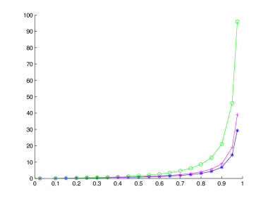
Figure 1: Expected queue length as a function of $\rho$. The curve for the E₂/M/1 queue is marked with $*$, for the M/M/1 queue with $+$ and for the H₂/M/1 with $\circ$.

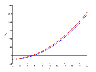
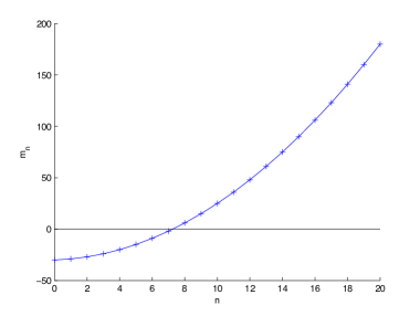
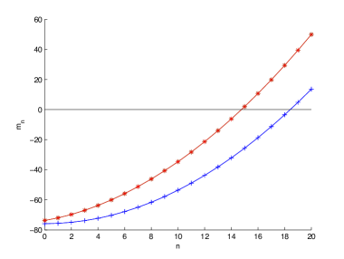
Figure 2: Queues E₂/M/1 (top), M/M/1 (middle) and H₂/M/1 (bottom); display of $m_{n,i}$ as a function of $n$ for each phase. The traffic coefficient is $\rho=1/1.2$. The blue curve (marked with “+”) is for phase 1, the red curve (marked with “*”) is for phase 2.

We take $\mu=1.2$ fixed, so that $L$ takes respectively the values 3.8, 5, and 11.1 for the Erlang, the exponential and the hyper-exponential arrival processes. We show on Figure 2 the components of the vectors ${\boldsymbol{m}}_{n}$ for small values of $n$. In all cases, the difference is increasing, starting from a negative value for small values of $n$, and becoming positive at some $n$ greater than $L$. We also observe a clear difference between the plots for the E₂/M/1 and the H₂/M/1 queues. Not surprisingly, the influence of the first phase is more pronounced in the latter case. Finally, the range of values for ${\boldsymbol{m}}_{n}$, $0\leq n\leq 20,$ is greater when the arrival distribution has a smaller variance, a feature that we did not expect.

Acknowledgment

It is a pleasant duty to mention that Bernd Heidergott and three anonymous referees have offered numerous and insightful comments on the first draft of this paper.

The authors thank the Ministère de la Communauté française de Belgique for funding this research through the ARC grant AUWB-08/13–ULB 5.

The third author also gratefully acknowledges the support of the Fundamental Research Funds for the Central Universities (grant number 2010QYZD001) and the National Natural Science Foundation of China (grant number 10901164).

Appendix

For the PH/M/1 queue, (21) becomes

$${\boldsymbol{y}}_{0} =L^{-1}{\boldsymbol{g}}_{0}-{\boldsymbol{1}}+A_{1}{\boldsymbol{y}}_{1}$$

$$=-{\boldsymbol{1}}+(1/\gamma)({\boldsymbol{\sigma}}{\boldsymbol{y}}_{1}){\boldsymbol{s}}$$

and (18) gives

$${\boldsymbol{m}}_{0} =(I-P_{*})^{\#}{\boldsymbol{y}}_{0}+c_{0}{\boldsymbol{1}}$$

$$=-\gamma(S+{\boldsymbol{s}}\,{\boldsymbol{\sigma}}G)^{\#}{\boldsymbol{y}}_{0}+c_{0}{\boldsymbol{1}}$$

$$=-({\boldsymbol{\sigma}}{\boldsymbol{y}}_{1})(S+{\boldsymbol{s}}\,{\boldsymbol{\sigma}}G)^{\#}{\boldsymbol{s}}+c_{0}{\boldsymbol{1}}$$

since $(S+{\boldsymbol{s}}\,{\boldsymbol{\sigma}}G)^{\#}{\boldsymbol{1}}={\boldsymbol{0}}$, which proves (50).

Equation (51) is merely a reformulation of (20), so that we only need to prove (52). Before doing so, we observe that

$$(I-U)^{-1}\sum_{n\geq 0}R^{n}{\boldsymbol{1}}=(I-U)^{-1}(I-R)^{-1}{\boldsymbol{1}}$$

and is equal to ${\boldsymbol{\tau}}_{1}$ by (25) — this proves (53) — and we also note that

$$\sum_{n\geq 0}nR^{n}{\boldsymbol{1}}=(I-R)^{-1}R(I-R)^{-1}{\boldsymbol{1}}=(I-R)^{-1}A_{1}{\boldsymbol{\tau}}_{1}$$

since $R=A_{1}(I-U)^{-1}$. By (20),

$${\boldsymbol{y}}_{n} =\sum_{0\leq i\leq n-1}G^{i}(I-U)^{-1}\sum_{k\geq 0}R^{k}(L^{-1}(n-i+k){\boldsymbol{1}}-{\boldsymbol{1}})$$

$$=L^{-1}\sum_{0\leq i\leq n-1}(n-i)G^{i}{\boldsymbol{\tau}}_{1}-\sum_{0\leq i\leq n-1}G^{i}{\boldsymbol{\tau}}_{1}$$

$$\quad+L^{-1}\sum_{0\leq i\leq n-1}G^{i}(I-U)^{-1}\sum_{k\geq 0}kR^{k}{\boldsymbol{1}}$$

from which (52) follows.

Finally, we need to determine $c_{0}$ such that ${\boldsymbol{\pi}}{\boldsymbol{m}}=0$. Observe that $\sum_{n\geq 0}{\boldsymbol{\pi}}_{n}G^{n}={\boldsymbol{\pi}}_{0}M$, where $M=\sum_{n\geq 0}R^{n}G^{n}$ is the unique solution of the linear system $M=I+RMG$ and may easily be computed. We immediately obtain from (50, 51) that

$$c_{0}=({\boldsymbol{\sigma}}{\boldsymbol{y}}_{1}){\boldsymbol{\pi}}_{0}M(S+{\boldsymbol{s}}\,{\boldsymbol{\sigma}}G)^{\#}{\boldsymbol{s}}-\sum_{n\geq 1}{\boldsymbol{\pi}}_{0}R^{n}{\boldsymbol{y}}_{n}.$$ (54)

To evaluate the last term, we proceed in three steps. Firstly, we write

$$\sum_{n\geq 1}R^{n}\sum_{0\leq i\leq n-1}G^{i} =\sum_{i\geq 0}\sum_{n\geq i+1}R^{n}G^{i}$$

$$=\sum_{i\geq 0}R^{i}\sum_{n\geq 1}R^{n}G^{i}$$

$$=\sum_{i\geq 0}R^{i}R(I-R)^{-1}G^{i}$$

$$=R(I-R)^{-1}M.$$

Secondly,

$$\sum_{n\geq 1}R^{n}\sum_{0\leq i\leq n-1}(n-i)G^{i} =\sum_{i\geq 0}R^{i}\sum_{n\geq i+1}(n-i)R^{n-i}G^{i}$$

$$=\sum_{i\geq 0}R^{i}\sum_{n\geq 1}nR^{n}G^{i}$$

$$=R(I-R)^{-2}M.$$

Finally, we use (52, 54) and find that

$$c_{0} =({\boldsymbol{\sigma}}{\boldsymbol{y}}_{1}){\boldsymbol{\pi}}_{0}M(S+{\boldsymbol{s}}\,{\boldsymbol{\sigma}}G)^{\#}{\boldsymbol{s}}-L^{-1}{\boldsymbol{\pi}}_{0}R(I-R)^{-2}M{\boldsymbol{\tau}}_{1}$$

$$\quad+{\boldsymbol{\pi}}_{0}R(I-R)^{-1}M{\boldsymbol{\tau}}_{1}$$

$$\quad-L^{-1}{\boldsymbol{\pi}}_{0}R(I-R)^{-1}M(I-U)^{-1}(I-R)^{-1}A_{1}{\boldsymbol{\tau}}_{1}.$$ (55)

References

• [1] E. Altman, C. Avrachenkov, and R. Núñez-Queija. Perturbation analysis for denumerable Markov chains with application to queueing models. Adv. Appl. Probab., 36:839–853, 2004.
• [2] S. Asmussen and M. Bladt. Poisson’s equation for queues driven by a Markovian marked point process. Queueing Syst., 17:235–274, 1994.
• [3] N. G. Bean, L. Bright, G. Latouche, C. E. M. Pearce, P. K. Pollett, and P. Taylor. The quasistationary behaviour of quasi-birth-and-death processes. Ann. Appl. Probab., 7:134–155, 1997.
• [4] S. Bhulai and F. M. Spieksma. On the uniqueness of solutions to the Poisson equations for average cost Markov chains with unbounded cost functions. Math. Meth. Oper. Res., 58:221–236, 2003.
• [5] D. A. Bini, G. Latouche, and B. Meini. Numerical Methods for Structured Markov Chains. Numerical Mathematics and Scientific Computation. Oxford University Press, Oxford, 2005.
• [6] S. L. Campbell and C. D. Meyer. Generalized Inverses of Linear Transformations. Dover Publications, New York, 1991. Republication.
• [7] X. Cao and H. Chen. Perturbation realization, potentials, and sensitivity analysis of Markov processes. IEEE Trans. Automatic Control, 42:1382–1393, 1997.
• [8] P. Coolen-Schrijner and E. A. van Doorn. The deviation matrix of a continuous-time Markov chain. Probab. Engrg. Informational Sci., 16:351–366, 2002.
• [9] P. Glynn. Poisson’s equation for the recurrent M/G/1 queue. Adv. Appl. Probab., 26:1044–1062, 1994.
• [10] B. Heidergott and A. Hordijk. Taylor series expansions for stationary Markov chains. Adv. Appl. Probab., 23:1046–1070, 2003.
• [11] Z. Hou and Y. Liu. Explicit criteria for several types of ergodicity of the embedded M/G/1 and GI/M/n queues. J. Appl. Probab., 41:778–790, 2004.
• [12] N. Kartashov. Strongly stable Markov chains. J. Soviet Math., 34:1493–1498, 1986.
• [13] G. Latouche, S. Mahmoodi, and P. G. Taylor. Level-phase independent stationary distributions for GI/M/1-type Markov chains with infinitely-many phases. Perfor mance Evaluation, to appear.
• [14] G. Latouche and V. Ramaswami. Introduction to Matrix Analytic Methods in S- tochastic Modeling. ASA-SIAM Series on Statistics and Applied Probability. SIAM, Philadelphia PA, 1999.
• [15] G. Latouche and P. G. Taylor. Drift conditions for matrix-analytic models. Math. Oper. Res., 28:346–360, 2003.
• [16] Y. Liu. Perturbation bounds for the stationary distributions of Markov chains. SIAM J. Matrix Anal. Appl., 33:1057–1074, 2012.
• [17] Y. Liu and Z. Hou. Several types of ergodicity for M/G/1-type Markov chains and Markov processes. J. Appl. Probab., 43:141–158, 2006.
• [18] A. M. Makowski and A. Shwartz. The Poisson equation for countable Markov chains: Probabilistic methods and interpretations. In E. A. Feinberg and A. Shwartz, editors, Handbook of Markov Decision Processes, pages 269–303. Kluwe Academic Publishers, Norwell, MA, 2002.
• [19] Y. Mao, Y. Tai, Y. Q. Zhao, and J. Zou. Ergodicity for the GI/G/1-type Markov chain. http://arxiv.org/abs/1208.5225, 2012.
• [20] C. D. Meyer. The role of the group generalized inverse in the theory of finite Markov chains. SIAM Rev., 17:443–464, 1975.
• [21] S. P. Meyn and R. L. Tweedie. Markov Chains and Stochastic Stability. Cambridge University Press, Cambridge, UK, second edition, 2009.
• [22] M. F. Neuts. Matrix-Geometric Solutions in Stochastic Models: An Algorithmic Approach. The Johns Hopkins University Press, Baltimore, MD, 1981.
• [23] V. Ramaswami and G. Latouche. An experimental evaluation of the matrix-geometric method for the GI/PH/1 queue. Comm. Statist. Stochastic Models, 5:629–667, 1989.
• [24] R. Syski. Ergodic potential. Stoch. Proc. Appl., 7:311–336, 1978.