Hybrid preconditioning for iterative diagonalization of ill-conditioned generalized eigenvalue problems in electronic structure calculations

Abstract

The iterative diagonalization of a sequence of large ill-conditioned generalized eigenvalue problems is a computational bottleneck in quantum mechanical methods employing a nonorthogonal basis for ab initio electronic structure calculations. We propose a hybrid preconditioning scheme to effectively combine global and locally accelerated preconditioners for rapid iterative diagonalization of such eigenvalue problems. In partition-of-unity finite-element (PUFE) pseudopotential density-functional calculations, employing a nonorthogonal basis, we show that the hybrid preconditioned block steepest descent method is a cost-effective eigensolver, outperforming current state-of-the-art global preconditioning schemes, and comparably efficient for the ill-conditioned generalized eigenvalue problems produced by PUFE as the locally optimal block preconditioned conjugate-gradient method for the well-conditioned standard eigenvalue problems produced by planewave methods.

1 Introduction

First principles (ab initio) quantum mechanical simulations based on density functional theory (DFT) [22, 25] are a vital component of research in condensed matter physics and molecular quantum chemistry. Using DFT, the many-body Schrödinger equation for the ground state properties of an interacting system of electrons and nuclei is reduced to the self-consistent solution of an effective single-particle Schrödinger equation, known as the Kohn-Sham equation:

$$\mathcal{H}\psi_{i}(r)=\left[-\frac{1}{2}\nabla^{2}+V_{\textrm{eff}}(r,\rho(r))\right]\psi_{i}(r)=\varepsilon_{i}\psi_{i}(r),$$ (1)

where $\varepsilon_{i}$ are particle energies (eigenvalues) and $\psi_{i}$ are the associated wavefunctions (eigenfunctions). The Hamiltonian $\mathcal{H}$ consists of kinetic energy operator $-\frac{1}{2}\nabla^{2}$ and effective potential operator $V_{\textrm{eff}}(r,\rho(r))$. The effective potential $V_{\textrm{eff}}$ depends on the electronic charge density

$$\rho(r)=\sum_{i}f_{i}|\psi_{i}(r)|^{2},$$ (2)

where $0\leq f_{i}\leq 2$ is the electronic occupation of state $i$ and the sum is over all occupied states. Since $\psi_{i}$ depends on $V_{\textrm{eff}}$ which depends on $\rho(r)$ which depends again on $\psi_{i}$, the Kohn-Sham equation (1) is a nonlinear eigenvalue problem.

The importance of ab initio calculations stems from their underlying quantum-mechanical nature, yielding insights inaccessible to experiment and robust, predictive power unattainable by more approximate empirical approaches. However, because ab initio calculations are computationally intensive, a vast range of real materials problems remain inaccessible by such accurate, quantum mechanical means. To address this limitation, there has been substantial effort in recent years to develop ab initio methods that use efficient, local bases in order to both reduce degrees of freedom and facilitate large-scale parallel implementation: augmented planewave plus local orbital (APW+lo) [49, 50], atomic-orbital (AO), e.g., [3, 8], and real-space methods [6, 55, 41] such as finite-difference [12, 13, 10], wavelet [14, 2, 18], finite-element (FE) [56, 36], partition-of-unity finite element (PUFE) [54, 38, 37], and discontinuous Galerkin (DG) [27] methods, among many others, see for example [30].

In the vast majority of ab initio methods, the dominant computational cost is the iterative diagonalization of the sequence of large linear eigenvalue problems produced by the discretization of equation (1) in the chosen basis [43, 26, 60, 42, 41, 61, 58, 40]. The linear eigenvalue problems produced by highly efficient physics based APW+lo, AO, and PUFE bases, while smaller than those of other bases, present a particular challenge as they are generalized eigenvalue problems with ill-conditioned coefficient matrices, and are much more difficult to precondition than those produced by conventional planewave based methods, due to the lack of diagonal dominance and absence of an efficient representation for the inverse Laplacian.

Here, building on prior work [59, 48, 34, 1, 40, 7], we propose a hybrid preconditioning scheme for rapid iterative diagonalization of the sequence of ill-conditioned generalized Hermitian eigenvalue problems produced by modern orbital based electronic structure methods, such as APW+lo, AO, and PUFE. The hybrid preconditioning scheme effectively combines a global shifted-inverse preconditioner as in [34, 1, 7] and locally accelerated shifted-inverse preconditioners as in [59, 48, 34, 1, 40] that target eigenpairs of interest individually. The global preconditioner serves as sole preconditioner in early self-consistent iterations and as convergence accelerator for local preconditioners in subsequent iterations. We have conducted extensive tests of the proposed hybrid preconditioning scheme with the block steepest descent method in PUFE pseudopotential density functional calculations on a variety of systems, including the difficult case of triclinic metallic CeAl. This system has deep atomic potentials and 15 electrons per unit cell in valence, thus requiring the computation of many, strongly localized eigenfunctions, which in turn requires the addition of correspondingly many orbital enrichments in the PUFE electronic structure method. Our results reveal that in terms of average numbers of inner and outer iterations, the hybrid preconditioner performs markedly better than global or local preconditioners alone, and the resulting solver performs as well on the ill-conditioned generalized eigenvalue problems produced by the PUFE ab initio method as does the locally optimal block preconditioned conjugate-gradient (LOBPCG) method on well-conditioned standard eigenvalue problems produced by the planewave method.

The remainder of the paper is organized as follows. In Section 2, we outline the self-consistent field (SCF) procedure and iterative diagonalization process in an algebraic setting, and discuss the ill-conditioned generalized eigenvalue problems produced by the PUFE electronic structure method. In Section 3, we describe the hybrid preconditioning scheme and its use in the block steepest descent method. Implementation details are presented in Section 4. Numerical results are presented in Section 5 and we close with final remarks in Section 6.

2 SCF, iterative diagonalization, and ill-conditioned GHEPs

Electronic structure methods such as APW+lo, AO, and PUFE methods incorporate information from local atomic solutions to construct efficient bases for molecular or condensed matter calculations. This information is typically incorporated in the form of localized, atomic-like basis functions (orbitals), which generally leads to a nonorthogonal basis. Discretization of the Kohn-Sham equation (1) in such a basis then leads to a nonlinear algebraic eigenvalue problem

$${H}(V_{\textrm{eff}})\Psi=S\Psi E,$$ (3)

where ${H}(V_{\textrm{eff}})$ is the discrete KS-Hamiltonian matrix and consists of a local part $H^{({\rm loc})}(V_{\textrm{eff}})$ and, when pseudopotentials [30] are employed, nonlocal part $H^{({\rm nl})}$:

$${H}(V_{\textrm{eff}})=H^{({\rm loc})}(V_{\textrm{eff}})+H^{({\rm nl})}.$$

$H^{({\rm loc})}(V_{\textrm{eff}})$ is a Hermitian matrix which depends on the effective potential $V_{\textrm{eff}}$, which in turn depends on the electronic density $\rho(r)$ computed from the eigenvectors $\Psi$. $H^{({\rm nl})}$ is a low-rank Hermitian matrix associated with the non-local part of the pseudopotential. $S$ is the overlap (Gram) matrix of the basis and is Hermitian positive-definite. The nonlocal matrix $H^{({\rm nl})}$ and overlap matrix $S$ are independent of $V_{\textrm{eff}}$, and hence do not depend on $\rho(r)$ or $\Psi$. In condensed matter calculations, it is required to sample the Brillouin zone [30] at a sufficient number of $\mathbf{k}$-points, making the above matrices complex Hermitian rather than real symmetric. In addition, for methods whose basis functions are localized, such as wavelet, FE, PUFE, DG, and (to a lesser extent) AO-type methods, the above matrices are sparse: for example, in the case of PUFE, having a few hundred nonzero entries per row, independent of problem size.

The nonlinear eigenvalue problem (3) is solved by fixed-point iteration (see [30]): starting with an initial guess for the input charge density $\rho^{\mathrm{in}}$ and associated effective potential $V_{\textrm{eff}}^{\mathrm{in}}$ and iterating until the difference between the input and output effective potentials, $V^{\rm in}_{\textrm{eff}}$ and $V^{\rm out}_{\textrm{eff}}$, is within a specified tolerance $\tau_{\rm scf}$; i.e., the process is terminated at the $i_{s}$-th iteration if

$$v_{\rm dif}^{(i_{s})}=\frac{\|V^{\rm out}_{\textrm{eff}}-V^{\rm in}_{\textrm{eff}}\|}{\|V^{\rm in}_{\textrm{eff}}\|}\leq\tau_{\rm scf}.$$ (4)

This process is known as a self-consistent field (SCF) procedure. A schematic of the SCF procedure is shown in Figure 2.1.

Figure 2.1: Self-consistent field (SCF) procedure.

At the $i_{s}$-th SCF iteration, with an approximate effective potential $\widetilde{V}_{\textrm{eff}}$ extrapolated from previous SCF iterations [39], the nonlinear eigenvalue problem (3) becomes the following linear generalized Hermitian eigenvalue problem (GHEP):

$$H^{(i_{s})}\Psi^{(i_{s})}=S\Psi^{(i_{s})}E^{(i_{s})},$$ (5)

where

$$H^{(i_{s})}=H^{({\rm loc})}(\widetilde{V}_{\textrm{eff}})+H^{({\rm nl})},$$

$H^{({\rm loc})}(\widetilde{V}_{\textrm{eff}})$ is a Hermitian matrix, $H^{({\rm nl})}$ is a low-rank Hermitian matrix, $S$ is Hermitian positive definite, and all matrices are sparse when arising from discretization in a localized basis such as PUFE. As the SCF iteration proceeds, changes in $\widetilde{V}_{\textrm{eff}}$, and thus $H^{({\rm loc})}(\widetilde{V}_{\textrm{eff}})$, $\Psi^{(i_{s})}$, and $E^{(i_{s})}$ become smaller and smaller until convergence to the specified tolerance is achieved.

Since in the first few SCF iterations $\widetilde{V}_{\textrm{eff}}$ is not yet well converged, the GHEP (5) need not be solved to high accuracy. All that is necessary is that the accuracy be sufficient to allow the outer SCF iteration to converge without incurring significant additional iterations relative to exact solution. As the SCF iterations proceed and $\widetilde{V}_{\textrm{eff}}$ converges, the accuracy requirement for the solution of the GHEP (5) increases. Specifically, from the previous SCF iteration, we have an estimate $\{\widehat{E}_{0},\widehat{\Psi}_{0}\}$ of the lowest $m$ eigenpairs with the maximum residual norm

$$\tau_{{\rm eig},0}^{(i_{s})}=\mbox{Res}_{\max}[\widehat{E}_{0},\widehat{\Psi}_{0}],$$ (6)

where if $\widehat{E}=\mbox{diag}(\widehat{\varepsilon}_{1},\widehat{\varepsilon}_{2},\ldots,\widehat{\varepsilon}_{m})$ and $\widehat{\Psi}=[\widehat{\psi}_{1},\widehat{\psi}_{2},\ldots,\widehat{\psi}_{m}]$ are approximate eigenpairs, then

$$\mbox{Res}_{\max}[\widehat{E},\widehat{\Psi}]=\max_{1\leq i\leq m}\mbox{Res}[\widehat{\varepsilon}_{i},\widehat{\psi}_{i}],$$

and $\mbox{Res}[\widehat{\varepsilon}_{i},\widehat{\psi}_{i}]$ is the relative residual norm for the approximate eigenpair $(\widehat{\varepsilon}_{i},\widehat{\psi}_{i})$ of GHEP (5):

$$\mbox{Res}[\widehat{\varepsilon}_{i},\widehat{\psi}_{i}]\equiv\frac{\|r_{i}\|}{\|H^{(i_{s})}\widehat{\psi}_{i}\|},$$ (7)

and $r_{i}=H^{(i_{s})}\widehat{\psi}_{i}-\widehat{\varepsilon}_{i}S\widehat{\psi}_{i}$.

Our objective at the $i_{s}$-th SCF iteration is to compute the improved estimate $\{\widehat{E}_{l},\widehat{\Psi}_{l}\}$ satisfying

$$\mbox{Res}_{\max}[\widehat{E}_{l},\widehat{\Psi}_{l}]\leq\tau_{{\rm eig},l}^{(i_{s})}$$ (8)

where the tolerance $\tau_{{\rm eig},l}^{(i_{s})}$ is chosen to achieve a desired reduction relative to $\tau_{{\rm eig},0}^{(i_{s})}$ and/or ${v_{\rm dif}^{(i_{s})}}$. In practice, one or two orders of magnitude reduction is typically sufficient for the SCF procedure to converge in a comparable number of iterations to exact solutions (i.e., reduction to zero).

Since during the course of the SCF iteration to convergence, a wide range of accuracies are required for the solution of the GHEP (5) and excellent approximations are available for all eigenpairs at each SCF iteration after the first few, iterative diagonalization methods such as Davidson [15] and steepest descent [28, 48] can be much more efficient than direct methods, especially as problem sizes increase and memory constraints become a significant concern. However, while iterative solution methods make much larger computations possible, diagonalization remains the key bottleneck in large-scale ab initio calculations. Due to the nonorthogonal basis sets employed in electronic structure methods such as APW+lo, AO, and PUFE, the resulting numerical eigenvalue problems can be ill-conditioned. In particular, $H^{(i_{s})}$ and $S$ coefficient matrices can be ill-conditioned and share a large common near-null subspace. Furthermore, there is in general no clear gap between the eigenvalues that are sought (i.e., occupied states) and the rest. Moreover, the ill-conditioning and difficulty of iterative diagonalization become especially pronounced as bases become saturated with orbital functions with long tails in order to attain high accuracy.

Table 2.1 shows the condition numbers $\kappa(H^{(1)})$ and $\kappa(S)$ of coefficient matrices $H^{(1)}$ and $S$, respectively, at the first SCF iteration of PUFE calculations of metallic CuAl, using HGH pseudopotentials [21]. There are two atoms in the triclinic unit cell, which is subject to Bloch-periodic boundary conditions [54]. The Brillouin zone is sampled at the $\Gamma$-point and at $\mathbf{k}=(0.12,-0.24,0.37)$. The lattice vectors for the unit cell are:

$$\mathbf{a}_{1} =a(1.00,\;0.02,\;-0.04),$$

$$\mathbf{a}_{2} =a(0.06,\;1.05,\;-0.08),$$

$$\mathbf{a}_{3} =a(0.10,\;-0.12,\;1.10),$$

with lattice parameter $a=5.7$ Bohr. The Cu and Al atoms are located at lattice coordinates $\boldsymbol{\tau}_{1}=(0.01,0.02,0.03)$ and $\boldsymbol{\tau}_{2}=(0.51,0.47,0.55)$, respectively. Total energy calculations with PUFE are carried out on a uniform $n_{0}\times n_{0}\times n_{0}$ cubic-order finite element mesh, $r_{e}$ is the enrichment support radius, and $n_{\rm dof}$ is the resulting dimension of the GHEP (5).

Table 2.1: Condition numbers of $H^{(1)}$ and $S$ matrices in PUFE calculations of CuAl as a function of enrichment support radius.

$n_{0}$	$r_{e}$	$n_{\rm dof}$	$\kappa(H^{(1)})$	$\kappa(S)$
6	0.0	1512	7.4e02	3.0e03
6	1.0	1532	6.5e07	3.5e08
6	2.0	1685	3.3e08	3.3e09
6	3.0	2112	5.6e09	6.2e10
6	4.0	2518	3.0e10	4.5e11

In Table 2.1, the classical FE method corresponds to the case of no orbital enrichment, i.e., $r_{e}=0$ [36]. In this case, both matrices $H^{(1)}$ and $S$ are well-conditioned. However, once $r_{e}>0$ and orbital enrichments are added, the condition numbers of $H^{(1)}$ and $S$ increase sharply. In addition, we observe that $H^{(1)}$ and $S$ share a large common near-null subspace. For example, when $n_{0}=6$ and $r_{e}=1.0$, there is a subspace of dimension $n_{e}=20$ spanned by the columns of an orthogonal matrix $V$ with $\|V\|=1$ such that $\|H^{(1)}V\|=\|SV\|=O(10^{-4})$. Furthermore, some eigenvalues are clustered and there is no obvious gap between the eigenvalues of interest and the rest. Figure 2.2 shows the lowest 8 (3% of the eigenvalues of $H^{(1)}$ and $S$) of interest and higher states in the vicinity.

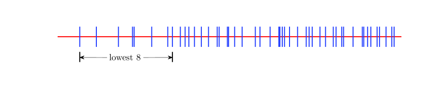
Figure 2.2: Partial distribution of energy eigenvalues for CuAl, showing the clustering and proximity of the lowest 8 computed values to the remainder of the spectrum.

Ill-conditioned generalized eigenvalue problems in quantum mechanical calculations with large nonorthogonal basis sets have been studied for decades, since the introduction of such bases, see for example [29, 23]. The challenges of solving ill-conditioned problems arising from the partition-of-unity FE method is an active research area, see for example [53, 19]. In the next section, we propose a hybrid preconditioning technique for the rapid iterative diagonalization of ill-conditioned GHEPs (5), as occur in orbital based ab initio methods such as APW+lo, AO, and PUFE.

3 Hybrid preconditioning and LABPSD

In this section, we consider the rapid iterative diagonalization of the GHEP (5). Specifically, we start with the approximates $\{\widehat{E}_{0},\widehat{\Psi}_{0}\}$ of the lowest $m$ eigenpairs of (5) from the previous SCF iteration. The objective at the $i_{s}$-th iteration is to compute improved approximate eigenpairs $\{\widehat{E}_{l},\widehat{\Psi}_{l}\}$ satisfying (8).

The block preconditioned steepest descent (BPSD) method [24], also known as a simultaneous Rayleigh quotient minimization method [28], proceeds as follows. Assume $\{\widehat{E}_{\ell-1},\widehat{\Psi}_{\ell-1}\}$ are obtained from $(\ell-1)$-st BPSD iteration with the residuals

$$R=H\widehat{\Psi}_{\ell-1}-S\widehat{\Psi}_{\ell-1}\widehat{E}_{\ell-1},$$

where for simplicity, the superscript $i_{s}$ of $H^{(i_{s})}$ is dropped here and in the remainder of this section. For the $\ell$-th approximate eigenpairs, we first compute search space vectors:

$$p_{i}=-{K}_{i}r_{i}\quad\mbox{for $i=1,2,\ldots,m$,}$$

where $r_{i}$ is the $i$th column of $R$, and $K_{i}$ is the corresponding preconditioner. $p_{i}$ is also called a preconditioned residual. Let $Z=[\widehat{\Psi}_{\ell-1}\;P]$ with $P=[p_{1},p_{2},\ldots,p_{m}]$, then the $\ell$-th approximate eigenpairs $\{\widehat{E}_{\ell},\widehat{\Psi}_{\ell}\}$ are obtained via the Rayleigh-Ritz procedure with the projection subspace matrix $Z$, i.e., $\widehat{E}_{\ell}=\Gamma$, $\widehat{\Psi}_{\ell}=ZW$, and $\{\Gamma,W\}$ are the lowest $m$ eigenpairs of the reduced matrix pair $({H}_{\rm R},{S}_{\rm R})=(Z^{H}HZ,Z^{H}SZ)$.

The convergence of the BPSD method depends critically on the preconditioners $K_{i}$. As we have discussed in Section 2, due to the nonorthogonal basis sets employed in electronic structure methods such as APW+lo, AO, and PUFE, the GHEP (5) can be ill-conditioned. It is well known that the presence of large off-diagonal entries in $H$ and $S$ from local orbital components of such bases render standard preconditioning techniques based on the diagonal of $H-\sigma S$ no longer effective [40, 7].

In the recent work of Blaha et al [7] on iterative diagonalization in the context of the APW+lo method, the following preconditioner is proposed:

$$K_{i}=(H-\bar{\varepsilon}S)^{-1}\equiv K_{\bar{\varepsilon}}\quad\mbox{for all $i$},$$ (9)

where $\bar{\varepsilon}$ is a parameter chosen close to the eigenvalues of interest, and the matrices $H$ and $S$ are chosen from a fixed (usually the first) SCF iteration and do not change in the entire SCF procedure. We call $K_{\bar{\varepsilon}}$ a global preconditioner. Such a global preconditioner has been proposed in the context of FE [1] and planewave [45] based methods as well.

To apply the global preconditioner (9), in [7], a dense LDL^T factorization of $K_{\bar{\varepsilon}}$ is first computed and stored on disk. During the entire SCF procedure, the factorization is read in to perform the required matrix-vector multiplications. In [1], in the context of an FE basis, the search space vectors $\{p_{i}\}$ are computed approximately by an iterative linear solver. Unfortunately, as we show in Section 5, such a preconditioner leads to stagnation in the context of less well-conditioned PUFE matrices.

In [59, 48, 34, 1, 40], the following preconditioners are proposed to individually target eigenpairs of interest:

$$K_{i}=(H-\widehat{\varepsilon}_{i}S)^{-1}\equiv K_{\widehat{\varepsilon}_{i}}\quad\mbox{for $i=1,2,\ldots,m$},$$ (10)

where $\widehat{\varepsilon}_{i}$ are Ritz values from the previous BPSD iteration, i.e., diagonal elements of $\widehat{E}_{\ell-1}$. The basic motivation can be understood as follows (e.g., [59, 48, 16]). Given current approximation $\{\widehat{\psi}_{i},\widehat{\varepsilon}_{i}\}$ to eigenpair $\{\psi_{i},\varepsilon_{i}\}$, we seek correction $p_{i}$ such that $\widehat{\psi}_{i}+p_{i}$ is exact, i.e.,

$$(H-\varepsilon_{i}S)(\widehat{\psi}_{i}+p_{i})=0.$$ (11)

While the exact eigenvalue $\varepsilon_{i}$ is unknown, the Rayleigh quotient

$$\widehat{\varepsilon}_{i}=\frac{\widehat{\psi}_{i}^{H}H\widehat{\psi}_{i}}{\widehat{\psi}_{i}^{H}S\widehat{\psi}_{i}}$$ (12)

provides an excellent approximation, with an error that is second order in the error of $\widehat{\psi}_{i}$. Replacing $\varepsilon_{i}$ with $\widehat{\varepsilon}_{i}$ in (11) then gives

$$(H-\widehat{\varepsilon}_{i}S)(\widehat{\psi}_{i}+p_{i})=r_{i}+(H-\widehat{\varepsilon}_{i}S)p_{i}=0$$ (13)

or

$$p_{i}=-(H-\widehat{\varepsilon}_{i}S)^{-1}r_{i},$$ (14)

as in (10). Note, however, that as $\widehat{\varepsilon}_{i}$ approaches $\varepsilon_{i}$, the matrix $H-\widehat{\varepsilon}_{i}S$ becomes singular and hence the inverse exists only in the subspace orthogonal to $\psi_{i}$ and any vectors degenerate with it [48, 16, 52]. Furthermore, for $\widehat{\varepsilon}_{i}\neq\varepsilon_{i}$, the inverse exists and returns the correction $p_{i}=-\widehat{\psi}_{i}$, providing no correction to the direction of $\widehat{\psi}_{i}$ whatsoever. In practice, since the inverse is computed only approximately, neither of these issues is a particular concern; however, they can affect convergence at higher accuracies [52]. In the present case, we solve the equation

$$(H-\widehat{\varepsilon}_{i}S)p_{i}=-r_{i},$$ (15)

inexactly, i.e., find $\widehat{p}_{i}$ satisfying

$$\|(H-\widehat{\varepsilon}_{i}S)\widehat{p}_{i}+r_{i}\|\leq\eta\|r_{i}\|,$$ (16)

where $\eta$ is a prescribed tolerance.

An asymptotic analysis of superlinear convergence of the preconditioner $K_{\widehat{\varepsilon}_{1}}$ for computing the smallest eigenpair has been studied in [44, 31]. This convergence analysis is extended for the case of multiple eigenpairs in our recent work [11]. Since the preconditioners $\{K_{\widehat{\varepsilon}_{i}}\}^{m}_{i=1}$ accelerate the convergence of individual eigenpairs $\{\widehat{\psi}_{i},\widehat{\varepsilon}_{i}\}$, we refer to them as locally accelerated preconditioners.

It is a computational challenge to apply the locally accelerated preconditioners at each BPSD iteration in a cost-effective way. In [40], it is suggested to first compute the full spectral decomposition of the matrix pair $(H,S)$ at some SCF iteration. However, the spectral decomposition is prohibitively expensive for large-scale systems. In [34, 1], the conjugate-gradient method is used for solving (15). This allows for very larger-scale calculations. However, the CG method (or MINRES for indefinite systems) suffers slow convergence and stagnation due to the ill-conditioning of the coefficient matrices, in the PUFE context in particular.

To overcome the slow convergence of higher eigenpairs using the global preconditioner and high computational cost and stagnation of the locally accelerated preconditioners, we propose the following hybrid preconditioning scheme:

1. In the initial few SCF iterations, apply only the global preconditioner $K_{\bar{\varepsilon}}$ to compute all search space vectors $P=[p_{1},p_{2},\ldots,p_{m}]$, i.e.,

   $$P=-K_{\bar{\varepsilon}}R=-(H-\bar{\varepsilon}S)^{-1}R.$$

2. If the $i$-th approximate eigenvalue $\widehat{\varepsilon}_{i}$ is localized, apply the locally accelerated preconditioner $K_{\widehat{\varepsilon}_{i}}$ in two stages:

   1. Compute an initial search space vector $\widehat{p}^{(0)}_{i}$ by applying the global preconditioner $K_{\bar{\varepsilon}}$:

      $$\widehat{p}^{(0)}_{i}=-K_{\bar{\varepsilon}}r_{i}=-(H-\bar{\varepsilon}S)^{-1}r_{i}.$$

   2. Iteratively refine $\widehat{p}^{(0)}_{i}$ to find the search space vector $\widehat{p}_{i}$ satisfying (16).

This two-stage application of locally accelerated preconditioners $K_{\widehat{\varepsilon}_{i}}$ addresses the issue of slow convergence of iterative methods for computing $\widehat{p}_{i}$. Using a good initial approximation $\widehat{p}^{(0)}_{i}$, the iterative refinement is expected to converge in just a few iterations, typically 2 to 5. The pre-application of the global preconditioner is efficient since the factorization of the global preconditioner is already available from the initial SCF iteration. As shown in Section 5, the proposed hybrid preconditioning scheme amortizes the cost of the global preconditioner and significantly reduces the cost of the more aggressive locally accelerated preconditioners, yielding a cost-effective preconditioning scheme for the iterative diagonalization of ill-conditioned GHEPs.

We shall refer to the combined algorithm, BPSD with above hybrid preconditioning, as the Locally Accelerated Block Preconditioned Steepest Descent (LABPSD) method. An outline of the method is as follows:

1. Input initial approximate eigenpairs $\{E,\Psi\}$, where $\Psi\in\mathbb{C}^{n\times(m+m_{0})}$

2. Compute ${\rm tol}_{0}=\mbox{Res}_{\max}[{E},{\Psi}]$

3. Compute matrix-vector products $\Psi_{H}=H\Psi$ and $\Psi_{S}=S\Psi$

4. Compute residual vectors $R={\Psi_{H}}_{(:,1:m)}-{\Psi_{S}}_{(:,1:m)}E_{(1:m,1:m)}$

5. Test for convergence to tolerance $\tau^{(i_{s})}_{\rm eig}$. If converged, exit

6. Set up search subspace $Z=[\Psi\,\,P]$ with preconditioned residual vectors $P$ computed as follows:

   (a) Apply global preconditioner: $P=-K^{(i_{0})}_{\bar{\varepsilon}}R$

   (b) If $\varepsilon_{i}=E_{(i,i)}$ is localized for some $i$ and $1\leq i\leq m$, refine $p_{i}=P_{(:,i)}$ with locally accelerated preconditioner, i.e., compute correction vector $\delta p_{i}$ by solving refinement equation

   $$(H-\varepsilon_{i}S)\delta p_{i}=-\delta{r}_{i}$$

   inexactly, where $\delta{r}_{i}=(H-\bar{\varepsilon}S)p_{i}+r_{i}$. Set $P_{(:,i)}:=p_{i}+\delta p_{i}$

7. Perform matrix-vector products $P_{H}=HP$ and $P_{S}=SP$

8. Set up coefficient matrices of reduced GHEP

   $$H_{\rm R}=[\Psi\,\,P]^{H}[\Psi_{H}\,\,P_{H}]\quad\mbox{and}\quad S_{\rm R}=[\Psi\,\,P]^{H}[\Psi_{S}\,\,P_{S}]$$

9. Compute lowest $m+m_{0}$ eigenpairs $\{W,E\}$ of $({H}_{\rm R},{S}_{\rm R})$:

   $${H}_{\rm R}W={S}_{\rm R}WE$$

10. Compute new approximate eigenvectors $\Psi:=[\Psi\,P]W$

11. Update $\Psi_{H}:=[\Psi_{H}\,P_{H}]W$ and $\Psi_{S}:=[\Psi_{S}\,P_{S}]W$

12. Go to step 4.

A few remarks are in order.

1. The initial approximations $\Psi$ are eigenvectors $\Psi^{(i_{s}-1)}$ from the previous SCF iteration, i.e., $\Psi=\Psi^{(i_{s}-1)}$. Having the extra $m_{0}$ vectors is important. It can accelerate convergence substantially when there are multiple (degenerate) or clustered eigenvalues at or near the $m$-th. In practical calculations (with multiplicities limited by symmetries in the underlying physical problem), a small $m_{0}$ is generally sufficient, for example $m_{0}=m/10$. The larger the $m_{0}$, the faster the convergence, but also the more matrix-vector products required. Similar findings pertain for other solvers in the electronic structure context as well, see for example [26, 40, 7].

2. The LABPSD iteration is considered to be converged if $\mbox{Res}_{\max}[{E}_{(1:m,1:m)},{\Psi}_{(:,1:m)}]\leq\tau^{(i_{s})}_{\rm eig}$.

3. Line 6 is only executed for residual vectors corresponding to unconverged eigenpairs. The implementation details are presented in Section 4.

4. The $i$-th approximate eigenpair $\{\varepsilon_{i},\psi_{i}\}=\{E_{(i,i)},{\Psi}_{(:,i)}\}$ is deemed “localized” if the following conditions are satisfied:

   $$\mbox{Res}[\varepsilon_{i},\psi_{i}]\leq\tau_{1}\quad\mbox{and}\quad|\varepsilon_{i}-\varepsilon^{\ell-1}_{i}|\leq\tau_{2}|\varepsilon^{\ell-1}_{i}|,$$

   where $\varepsilon^{\ell-1}_{i}$ is the $i$-th approximate eigenvalue from the previous ($\ell-1$) BPSD iteration. Both $\tau_{1}$ and $\tau_{2}$ are parameters. In our numerical tests, we set $\tau_{1}=\tau_{2}=0.1$. The above localization condition thus provides an indication that the $i$-th approximate eigenvalue $\varepsilon_{i}$ has settled down sufficiently with respect to BPSD iterations $\ell$ to be used as a shift for preconditioning.

5. By storing the block vectors $\Psi_{H}$, $\Psi_{S}$, $P_{H}$ and $P_{S}$, the matrices $H$ and $S$ are accessed only once per BPSD iteration, other than in preconditioning step 6.

6. The reduced dense GHEP $({H}_{\rm R},{S}_{\rm R})$ can be solved by standard routines such as LAPACK ZHEGVX.

4 Implementation details

In this section, we discuss implementation details of the hybrid preconditioning scheme in step 6 of the LABPSD method.

First, we consider the global preconditioning step 6(a). As discussed in Section 3, the global preconditioner $K_{\bar{\varepsilon}}$ is fixed throughout the SCF iterations. Typically, the coefficient matrices $H^{(1)}$ and $S$ in the first SCF iteration are sufficient to construct an effective $K_{\bar{\varepsilon}}$, i.e., $i_{0}=1$ in line 6(a) of LABPSD. Therefore, let us consider how to exploit the structure of $H^{(1)}$ and $S$ to efficiently compute

$$P=-K^{(1)}_{\bar{\varepsilon}}R=-\left(H^{(1)}-\bar{\varepsilon}S\right)^{-1}R.$$ (17)

From the definition (5) of $H^{(1)}$, the global preconditioner $K^{(1)}_{\bar{\varepsilon}}$ is the inverse of a Hermitian matrix plus low-rank update:

$$K^{(1)}_{\bar{\varepsilon}}=\left(H^{({\rm loc},1)}-\bar{\varepsilon}S+H^{({\rm nl})}\right)^{-1},$$ (18)

where $H^{({\rm loc},1)}-\bar{\varepsilon}S$ is Hermitian and $H^{({\rm nl})}$ has the rank-revealing decomposition

$$H^{({\rm nl})}=FGF^{H},$$ (19)

where $F$ is $n$-by-$k$ and $G$ is $k$-by-$k$ Hermitian. The rank $k$ is the number of projectors in the pseudopotential formulation, typically $k\ll n$. For localized bases such as PUFE, $H^{({\rm loc},1)}$ and $S$ are sparse.

To compute $P$, we first compute the following factorization of the matrix $H^{({\rm loc},\;1)}-\bar{\varepsilon}S$:

$$\Pi^{\top}(H^{({\rm loc},\;1)}-\bar{\varepsilon}S)\Pi=LDL^{H},$$ (20)

where $\Pi$ is a permutation matrix, $L$ is a unit lower triangular matrix, and $D$ is a block diagonal matrix with only 1-by-1 and 2-by-2 blocks on the diagonal. Algorithms for the factorization (20) are well-established, see for example [46, 47, 17]. Since the global preconditioner is unchanged during the SCF iterations, the factorization (20) is computed just once and used throughout the SCF process. This is along the lines of the global preconditioning scheme suggested in [7]. However, in the context of a localized basis and sparse matrices, such as PUFE, we use a sparse factorization rather than dense one as in [7].

With the low-rank representation (19) and factorization (20), we can compute the global-preconditioned search space vectors $P$ using the Sherman-Morrison-Woodbury (SMW) formula [20] as follows:

1. Compute $\widehat{F}=(H^{({\rm loc},\;1)}-\bar{\varepsilon}S)^{-1}F$ using the factorization (20)

2. $F:=FG$

3. $T=I+F^{H}\widehat{F}$

4. $F:=FT^{-H}$

5. Compute $P=-(H^{({\rm loc},\;1)}-\bar{\varepsilon}S)^{-1}R$ using the factorization (20)

6. $P:=P-\widehat{F}F^{H}P$

Here we have arranged the order of computations such that the first four steps are executed just once. By storing $F$ and $\widehat{F}$, $P$ can be computed using only the last two steps.

Turning now to the locally accelerated preconditioning step 6(b), the iterative refinement of initial approximate $\widehat{p}^{(0)}_{i}=P_{(:,i)}$ computed in step 6(a) can be recast as solving the following linear system:

$$(H^{(i_{s})}-\varepsilon_{i}S){p}_{i}=-r_{i},$$ (21)

with starting vector $\widehat{p}^{(0)}_{i}$. Since $H^{(i_{s})}-\varepsilon_{i}S$ is Hermitian and indefinite, MINRES [33, 57] is a natural choice. Although the coefficient matrix $H^{(i_{s})}-\varepsilon_{i}S$ of (21) can become highly ill-conditioned, as we show below, we observe that it takes just 2 to 5 iterations for MINRES to converge to the desired tolerance starting from the pre-processed vectors $\widehat{p}^{(0)}_{i}$ from the global preconditioner.

5 Results

In this section, we provide numerical results to demonstrate the efficiency of the LABPSD algorithm for the rapid iterative diagonalization of ill-conditioned generalized eigenvalue problems produced by the PUFE electronic structure method [54, 38, 37], which employs a strictly local nonorthogonal basis combining atomic orbitals for efficiency and finite elements for generality and systematic improvability.

We have conducted extensive tests of the LABPSD method in PUFE calculations of a variety of materials systems. Here we show results for two systems representative of opposite extremes: CuAl with a soft, shallow pseudopotential and clustered or degenerate eigenvalues, and CeAl with a notably hard and deep pseudopotential and nondegenerate spectrum.

CuAl

Our first test case is a high-symmetry, cubic CuAl metallic system, with $\Gamma$-point Brillouin zone sampling to maximize degeneracies in the spectrum. The unit cell is body-centered cubic with lattice parameter $a=5.8$ Bohr and atomic positions $\boldsymbol{\tau}_{1}=(0.0,0.0,0.0)$ (Cu) and $\boldsymbol{\tau}_{2}=(0.5,0.5,0.5)$ (Al), in lattice coordinates. The Brillouin zone is sampled at the $\Gamma$-point to maximize degeneracies in the spectrum, including degeneracy at the Fermi level, thus providing a stringent test of the eigensolver’s ability to extract clustered/degenerate eigenpairs. The resulting spectrum has a triple-degeneracy (eigenvalues of $0.36047$ Hartree) and a double-degeneracy (eigenvalues of $0.37553$ Hartree), which is also the highest occupied state with Fermi-Dirac occupation and $k_{B}T=0.01$ a.u.

CeAl

As a test of the solver’s ability to handle general, nondegenerate spectra, with low-lying eigenvalues and thus broader overall spectrum, we consider next the case of metallic, triclinic CeAl. This is a particularly challenging system due to the following properties: (a) The potentials of the atoms are deep, producing strongly localized solutions, with low-lying eigenvalues, that require larger basis sets to resolve. (b) The atoms are heavy, with many electrons in valence, requiring many eigenfunctions to be computed. (c) Because the system contains Ce, it requires 17 orbital enrichment functions per atom (in contrast to Cu for example, which requires only 1), which increases basis size substantially for PUFE. The radial parts of the orbital enrichment functions (pseudoatomic wavefunctions) for Ce and Al are shown in Figure 5.3. (d) The lattice is triclinic with atoms displaced from ideal positions. This provides a completely general problem, with no special symmetries to exploit and general, nondegenerate spectrum. (e) We do not assume a band gap, but rather solve the general metallic problem with Fermi-Dirac occupation and $k_{B}T=0.01$ a.u.

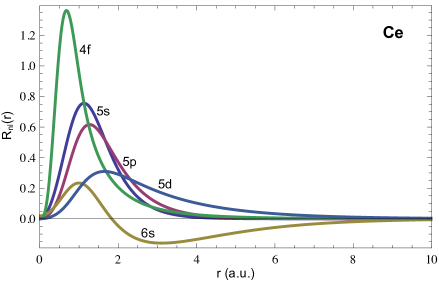
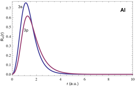
Figure 5.3: PUFE orbital enrichment functions for CeAl. Radial parts for (a) Ce and (b) Al.

The triclinic unit cell for CeAl has lattice vectors

$$\mathbf{a}_{1} =a(1.00,\;0.02,\;-0.04),$$

$$\mathbf{a}_{2} =a(0.01,\;0.98,\;0.03),$$

$$\mathbf{a}_{3} =a(0.03,\;-0.06,\;1.09),$$

with lattice parameter $a=5.75$ Bohr. Atomic lattice coordinates are $\boldsymbol{\tau}_{1}=(0.01,0.02,0.03)$ (Ce) and $\boldsymbol{\tau}_{2}=(0.51,0.47,0.55)$ (Al). The Brillouin zone is sampled at the $\Gamma$-point and at $\mathbf{k}=(0.12,-0.24,0.37)$. Therefore, there are two independent sequences of GHEPs in the SCF procedure.

For all simulations, the SCF procedure is terminated at the $i_{s}$-th iteration if the relative change of input and output effective potentials satisfies

$$v_{\rm dif}^{(i_{s})}=\frac{\|V^{\rm out}_{\textrm{eff}}-V^{\rm in}_{\textrm{eff}}\|}{\|V^{\rm in}_{\textrm{eff}}\|}\leq\tau_{\rm scf}$$ (22)

for a prescribed tolerance $\tau_{\rm scf}$. As reference, total energies are also calculated by the abinit planewave code [9] with well-converged planewave cutoff. By virtue of the orbital functions in the PUFE basis, the dimension of the PUFE GHEP is about a factor of 5 smaller than that of a planewave calculation of the same accuracy.

The dimension of the GHEP (5) is $n_{\rm dof}=7n_{0}^{3}+n_{e}$, where $n_{0}$ is the number of elements the $x$-, $y$- and $z$-directions (uniform FE mesh) and $n_{e}$ is determined by the enrichment support radius $r_{e}$ and number of atoms. The factor of 7 is due to the use of cubic serendipity brick elements [54]. By introducing a shift $\sigma_{0}$, $H^{(i_{s})}:=H^{(i_{s})}-\sigma_{0}S$ is made Hermitian positive definite. The PUFE code provides the routines to perform the matrix-vector multiplications $H^{({\rm loc})}v$, $H^{({\rm nl})}v$ and $Sv$ for an arbitrary vector $v$. Subsequently, the matrix-vector multiplication $(H^{(i_{s})}-\sigma S)v$ is readily computable for any shift $\sigma$ to facilitate preconditioning.

In addition, termination criteria for the SCF, BPSD, and MINRES iterations are $\tau_{\rm scf}=10^{-5}$, $\tau^{(i_{s})}_{\rm eig}=\frac{1}{10}v^{(i_{s})}_{\rm dif}$, and $\eta^{(i_{s})}=\eta=0.25$, respectively. The maximum number of outer BPSD and inner MINRES iterations are set to 20, unless otherwise specified. The outermost SCF iterations are repeated until convergence of the potential as defined in (22) is achieved. The global shift $\bar{\varepsilon}$ is chosen to be close to the desired eigenvalues of $(H^{(i_{s})},S)$. In particular, $\bar{\varepsilon}=-0.3$ for CuAl, $\bar{\varepsilon}=-1.0$ for CeAl, which are smaller than the estimated smallest eigenvalues of $(H^{(i_{s})},S)$ for the cases considered here. As observed in [7], our numerical experiments also show $\bar{\varepsilon}$ has little influence on the convergence of the BPSD iteration.

Computations reported in this paper were carried out on a two-socket six-core Intel Xeon 2.93 GHz processor with 94 GB memory. Intel MKL was used for BLAS and LAPACK operations in the LABPSD method. In addition, the DSS package of MKL was used for computing the sparse factorization (20) of the global preconditioner. DSS is an interface to PARDISO [46, 47] and provides subroutines to compute $(H^{({\rm loc},1)}-\bar{\varepsilon}S)^{-1}v$ for a given vector $v$ after the sparse factorization is computed.

5.1 SCF convergence

We first examine the convergence of the SCF procedure using LABPSD for the iterative diagonalization of the associated sequence of GHEPs.

CuAl

A uniform $12\times 12\times 12$ finite-element mesh and enrichment support radius $r_{e}=4$ are employed to provide high accuracy and a strong test of ill-conditioning. The dimension of the GHEP (5) is $n_{\rm dof}=7\times 12^{3}+8130=20226$. The rank of $H^{(\rm nl)}$ is $k=19$. $m=10$ eigenpairs are computed in order to accommodate all electrons in valence and achieve convergence of the effective potential to the desired accuracy.

The left plot of Figure 5.4 shows the maximum relative residual errors $\mbox{Res}_{\max}[\widehat{E},\widehat{\Psi}]$ of the sequence of the GHEPs at the beginning and end of each SCF iteration, where $m_{0}=10$ for the BPSD iterations. The right plot of Figure 5.4 shows the corresponding difference $v^{(i_{s})}_{\rm dif}$ of input and output effective potentials (Eq. (4)). As can be seen, with LAPBSD as the eigensolver, the maximum relative residual error of the GHEP steadily drops at the rate $\tau^{(i_{s})}_{\rm eig}=\frac{1}{10}v^{(i_{s})}_{\rm dif}$, along with the input-output potential difference. If the accuracy of the eigensolves at each SCF iteration is further increased, the convergence of the effective potential is not substantially affected.

We note that in the final SCF iteration, the lowest 10 computed eigenvalues are

-0.1987515094,	0.3604669213,	0.3604669241,	0.3604669358,	0.3755287169,
0.3755287473,	0.5721570004,	0.8464957683,	0.8464958151,	0.8464958184,

with triply degenerate value at $\sim 0.3604669$ and doubly degenerate value at $\sim 0.3755287$, as in the reference planewave calculations (deviations from exact degeneracy in the final digits are due to the lower symmetry of the basis than the crystal [35]). As can be seen, the degenerate values pose no particular difficulty for the LABPSD solver.

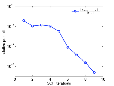
Figure 5.4: CuAl simulation. The maximum relative backward error of the sequence of GHEPs in the solution of NLEP (3) (left), and the relative difference of effective potentials $V_{\textrm{eff}}$ (right).

CeAl

For the CeAl system, we consider a $12\times 12\times 12$ finite-element mesh with $r_{e}=2.5$. The dimension of the GHEP (5) is $n_{\rm dof}=23795$. The rank of $H^{(\rm nl)}$ is $k=26$. In this case, $m=22$ eigenpairs are computed to accommodate all valence electrons with specified Fermi-Dirac occupation. The left plot of Figure 5.5 shows the reduction of the maximum relative residual errors $\mbox{Res}_{\max}[\widehat{E},\widehat{\Psi}]$ of the sequence of the GHEPs, where $m_{0}=3$. The right plot of Figure 5.5 shows the corresponding difference $v^{(i_{s})}_{\rm dif}$. Again, the maximum relative residual error of the GHEP steadily drops at the rate $\tau^{(i_{s})}_{\rm eig}=\frac{1}{10}v^{(i_{s})}_{\rm dif}$, along with the input-output potential difference.

If the accuracy of the eigensolves at each SCF iteration is further increased, the convergence of the effective potential is not substantially affected.

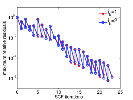
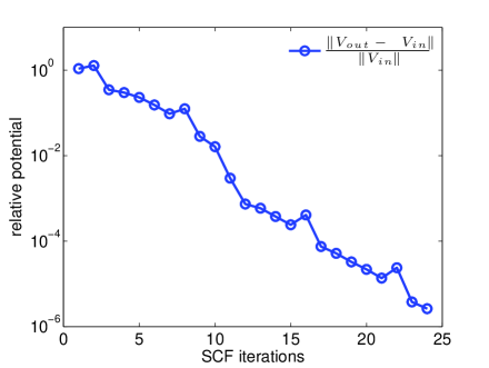
Figure 5.5: CeAl simulation. The maximum relative backward error of two sequences ($i_{k}=1$ and $i_{k}=2$) of GHEPs in the solution of NLEP (3) (left), and the relative difference of effective potentials $V_{\textrm{eff}}$ (right).

5.2 Inner and outer iterations

Now, let us examine the efficiency of the LABPSD in terms of the following two quantities:

$${\rm Hp}=\frac{B_{s}}{S_{s}\times N_{k}}\quad\mbox{and}\quad{\rm La}=\frac{M_{s}}{B_{s}\times m},$$

where $S_{s}$ is the total number of SCF iterations, $B_{s}$ is the total number of BPSD iterations, and $M_{s}$ is the total number of MINRES iterations. $N_{k}$ is the number of $\mathbf{k}$-points ($N_{k}=1$ in the CuAl case, $N_{k}=2$ in the CeAl case). By the above definition, ${\rm Hp}$ is the average number of outer BPSD iterations per SCF iteration for each $\mathbf{k}$-point. A small ${\rm Hp}$-number indicates the efficiency of the hybrid preconditioning technique. Similarly, ${\rm La}$ is the average number of inner MINRES iterations per outer BPSD iteration for each eigenpair. A small ${\rm La}$-number indicates the efficiency of applying the locally accelerated preconditioners in the proposed two stages.

CuAl

The left plot of Figure 5.6 shows the ${\rm Hp}$- and ${\rm La}$-numbers for LABPSD for a sequence of refined FE meshes with $r_{e}=4$ fixed. The right plot is for different enrichment support radii $r_{e}$ and fixed $8\times 8\times 8$ FE mesh. This constitutes a severe test of robustness with respect to ill-conditioning since as either the mesh or support radius are increased, the conditioning of the GHEP worsens dramatically, as shown in Table 2.1. In all cases, the rank of $H^{(\rm nl)}$ is $k=19$ and the number of eigenpairs computed per SCF iteration is $m=10$.

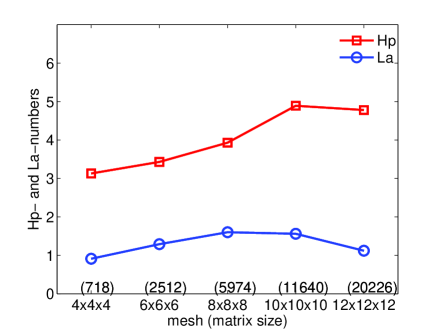
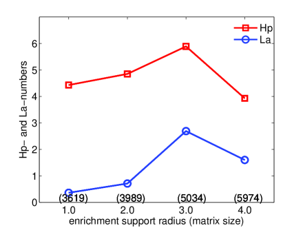
Figure 5.6: CuAl simulation: Hp- and La- numbers (see text) for the LABPSD solver for a series of $n_{0}\times n_{0}\times n_{0}$ FE meshes (left) and enrichment support radii $r_{e}$ (right).

CeAl

Similarly, for the CeAl system, the left plot of Figure 5.7 shows the ${\rm Hp}$- and ${\rm La}$-numbers with $r_{e}=2.5$. The right plot is for different enrichment support radii $r_{e}$ with the fixed $8\times 8\times 8$ FE mesh. This constitutes a severe test of robustness with respect to ill-conditioning. In this case, the rank of $H^{(\rm nl)}$ is $k=26$ and the number of eigenpairs computed per SCF iteration is $m=22$.

For both CuAl and CeAl simulations, as the mesh is refined or $r_{e}$ is increased, the error of the computed PUFE total energy decreases to $10^{-6}$ Hartree/atom relative to the well-converged planewave reference. Significantly, we observe that all Hp-numbers are between 2 and 6, with only mild dependence on conditioning as it worsens considerably with increasing mesh and support radius. Meanwhile, all La-numbers are between 0 and 4, with no apparent dependence on conditioning. As we show below (Section 5.4), this is in stark contrast to typical global-only or local-only preconditioning schemes, which are highly sensitive to the conditioning of the problem. Furthermore, these Hp- and La-numbers are comparable to the typical numbers of inner and outer iterations required by the LOBPCG method on the well-conditioned standard eigenvalue problems produced by the planewave ab initio method [9]. This indicates that LABPSD is an efficient method for the rapid iterative diagonalization of ill-conditioned GHEPs produced by nonorthogonal atomic-orbital based methods such as PUFE.

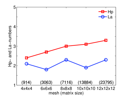
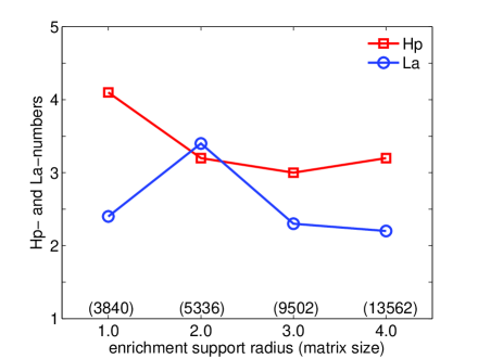
Figure 5.7: CeAl simulation, Hp- and La- numbers (see text) for the LABPSD solver for a series of $n_{0}\times n_{0}\times n_{0}$ FE meshes (left) and enrichment support radii $r_{e}$ (right).

5.3 Timing

We now consider the timing of key steps of LABPSD for increasing numbers $m$ of eigenpairs. For these purposes, we now focus on the more computationally intensive CeAl system, where the dimension of the GHEPs (5) is $n_{\rm dof}=7\times 12^{3}+11699=23795$. The enrichment support radius is $r_{e}=2.5$. The rank of $H^{(\rm nl)}$ is $k=26$.

Figure 5.8 shows the CPU time normalized with respect to the CPU time for computing $m=50$ eigenvalues, and the most time consuming parts for LABPSD are shown for a series of PUFE calculations with increasing numbers of eigenpairs $m=50,100,200$ with $m_{0}=10$. Each calculation takes 23 SCF iterations to converge to the required tolerance. As expected, the CPU time is dominated by the preconditioning step 6 at about 60% of the total time in all cases. The cost of the global preconditioner in step 6(a) increases as $m$ increases, as expected. However, as a percentage of the total, the cost actually decreases, which is a consequence of the fact that the cost of the sparse factorization (20) and application of the global preconditioner is amortized when more eigenpairs are computed. On the other hand, the cost of the locally accelerated preconditioners in step 6(b) increases as a percentage of the total as more eigenpairs are computed. The cost of matrix-vector products in step 7 is proportionally increased with the number of computed eigenpairs; however, the overall cost is reduced from 20% to about 15% of the total when more eigenpairs are computed. The costs of all other steps, such as setting up the reduced GHEP (step 8), updating (step 11), and solving the reduced eigenvalue problem (step 9) are relatively small at 20% of the total. As $m$ is increased further, the solution of the reduced problem must dominate at some point due to its $m^{3}$ scaling. However, at the present system sizes, it remains a small fraction of the total. Overall, when LABPSD is used for computing 4 times more eigenpairs, namely from $m=50$ to $m=200$, the total CPU time is also increased by about a factor of 4 (3.73).

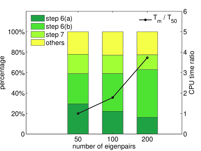
Figure 5.8: Normalized CPU time and percentages with increasing $m$ in the CeAl simulation.

We note that the $LDL^{\mathrm{H}}$ factorization (20) is computed only once at the beginning of the SCF cycle. The CPU time of the factorization (20) is a small percentage of the total. Specifically, the $LDL^{\mathrm{H}}$ factorizations for the two $\mathbf{k}$-points take just 3% of the total time when $m=50$, and 0.7% when $m=200$.

5.4 Global, local, and hybrid preconditioning

Here we compare the hybrid preconditioning scheme to current state-of-the-art global preconditioning as in [7] and local preconditioning as in [34, 1, 40]. Having demonstrated in Sections 5.1 and 5.2 the robustness of the hybrid preconditioner with respect to both the distribution (clustered and nonclustered) and width (hard and soft potentials) of the spectrum, we shall restrict focus here to the more computationally intensive CeAl system, where the dimension of the GHEPs is $n=7\times 8^{3}+3532=7116$. The enrichment support radius $r_{e}=2.5$, the rank of $H^{\rm(nl)}$ is $k=26$, and $m=22$ eigenpairs are computed at each SCF iteration with $m_{0}=3$.

Figure 5.9 shows the maximum relative residual norms of the eigenpairs in successive SCF iterations when solving the sequence of GHEPs by BPSD with global, local, and hybrid preconditioners.

If we use the global preconditioner step 6(a) only (i.e., without step 6(b)), the SCF convergence stagnates after about 9 SCF iterations due to the inability of the eigensolver to reduce residuals sufficiently within the maximum 200 BPSD iterations. The total CPU time was 11.4 hours, due to the relative ineffectiveness of the global preconditioner and consequent large number of outer (BPSD) iterations.

On the other hand, if we apply the local preconditioner step 6(b) only, without the global preconditioner 6(a), the SCF convergence stagnates after about 17 SCF iterations, again due to the inability of the eigensolver to reduce the residuals sufficiently even with the maximum 100 BPSD and 500 MINRES iterations. Due to the large number of both inner (MINRES) and outer (BPSD) iterations, the total CPU time was 138.6 hours.

In stark contrast, the SCF iteration converges steadily to the specified tolerance with the hybrid preconditioning scheme. The ${\rm Hp}$- and ${\rm La}$-numbers are 3.0 and 2.3, respectively, while achieving smooth SCF convergence at a rate comparable to exact diagonalization at each SCF step. Due to the small number of both inner and outer iterations, the total CPU time was reduced to just 1.3 hours.

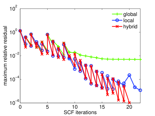
Figure 5.9: Maximum relative residual norms of GHEPs at the beginning and end of each SCF iteration, using global, local, and hybrid preconditioners in the CeAl simulation.

6 Conclusions

We proposed a block hybrid-preconditioned steepest descent method, LABPSD, for the iterative diagonalization of the sequence of ill-conditioned generalized Hermitian eigenvalue problems which arise in electronic structure calculations using orbital-based nonorthogonal basis sets. For such problems, the hybrid scheme overcomes the drawbacks of stagnation of global preconditioners and excessive cost of locally accelerated iterative preconditioners. PUFE pseudopotential density-functional calculations of CuAl, with soft potentials and degenerate eigenvalues, and CeAl, with hard potentials and nondegenerate spectrum, showed Hp- and La-numbers comparable to the typical numbers of inner and outer iterations required by the LOBPCG method on well-conditioned standard eigenvalue problems produced by the planewave ab initio method. Given the generality of the method and robustness with respect to spectral structure, it is expected that the LABPSD method will provide similar benefits to other orbital-based, nonorthogonal electronic structure methods as well. Indeed, it is reasonable to expect benefits not only for pseudopotential based methods, as demonstrated here, but for all-electron methods such as APW+lo [49] and LMTO [51] also, since these require diagonalization for just valence states as well (the core states having been solved separately in a spherical approximation).

The LABPSD algorithm and implementation present many opportunities for future work. First, similar to [7], we expect that the sparse $LDL^{\rm H}$ factorization (20) in single precision or even an incomplete factorization might be sufficient. This will substantially reduce memory and I/O costs for very large systems. Secondly, instead of using MINRES for the iterative refinement in applying locally accelerated preconditioners, one can use a simple first-order one-step iterative method [4]:

$$\widehat{p}^{(\ell+1)}_{i}=\widehat{p}^{(\ell)}_{i}-\alpha\left[(H^{(i_{s})}-\widehat{\varepsilon}_{i}S)\widehat{p}^{(\ell)}_{i}-r_{i}\right]$$

with initial $\widehat{p}^{(0)}_{i}$ from the global preconditioner, where $\alpha$ is chosen to minimize the residual norm of the linear system (15). Our preliminary results are very encouraging, which is particularly promising for parallel distributed computing. In addition, although we have not encountered the rank deficiency of the subspace matrix $Z$ produced in step 6 of the LABPSD method, a rank-revealing re-orthogonalization process would be necessary for a general-purpose implementation, such as in the block steepest descent method implemented in EA19 of HSL [32].

Acknowledgments. We are grateful to anonymous referees for their careful reading of the manuscript and most valuable comments.

References

- [1] K. E. Andersen. Electronic structure of nanomaterials: Computational methods and application to niobium clusters. PhD thesis, University of California, Davis, CA, U.S.A., 2005.
- [2] T. A. Arias. Multiresolution analysis of electronic structure: Semicardinal and wavelet bases. Rev. Mod. Phys., 71(1):267–311, 1999.
- [3] E. Artacho, E. Anglada, O. Diéguez, J. D. Gale, A. García, J. Junquera, R. M. Martin, P. Ordejón, J. M. Pruneda, D. Sánchez-Portal, and J. M. Soler. The SIESTA method; developments and applicability. J. Phys.: Cond. Matter, 20(6), 2008. 2nd Workshop on Theory Meets Industry, Erwin Schrodinger Inst, Vienna, Austria, Jun 12-14, 2007.
- [4] O. Axelsson. Iterative solution methods. Cambridge University Press, New York, 1994.
- [5] Z. Bai, J. Demmel, J. Dongarra, A. Ruhe, and H. van der Vorst (editors). Templates for the Solution of Algebraic Eigenvalue Problems: A Practical Guide. SIAM, Philadelphia, 2000.
- [6] T. L. Beck. Real-space mesh techniques in density functional theory. Rev. Mod. Phys., 72(4):1041–1080, 2000.
- [7] P. Blaha, H. Hofstätter, O. Koch, R. Laskowski, and K. Schwarz. Iterative diagonalization in augmented plane wave based methods in electronic structure calculations. J. Comput. Phys., 229(2):453–460, 2010.
- [8] V. Blum, R. Gehrke, F. Hanke, P. Havu, V. Havu, X. Ren, K. Reuter, and M. Scheffler. Ab initio molecular simulations with numeric atom-centered orbitals. Comput. Phys. Commun., 180(11):2175–2196, 2009.
- [9] F. Bottin, S. Leroux, A. Knyazev, and G. Zérah. Large-scale ab initio calculations based on three levels of parallelization. Comput. Mater. Sci., 42(2):329 – 336, 2008.
- [10] E. L. Briggs, D. J. Sullivan, and J. Bernholc. Large-scale electronic-structure calculations with multigrid acceleration. Phys. Rev. B, 52(8):R5471–R5474, 1995.
- [11] Y. Cai, Z. Bai, and N. Sukumar. A locally accelerated block preconditioned steepest descent method for generalized Hermitian eigenvalue problems. in preparation, 2012.
- [12] J. R. Chelikowsky, N. Troullier, and Y. Saad. Finite-difference pseudopotential method: Electronic-structure calculations without a basis. Phys. Rev. Lett., 72(8):1240–1243, 1994.
- [13] J. R. Chelikowsky, N. Troullier, K. Wu, and Y. Saad. Higher-order finite-difference pseudopotential method: An application to diatomic molecules. Phys. Rev. B, 50(16):11355–11364, 1994.
- [14] K. Cho, T. A. Arias, J. D. Joannopoulos, and P. K. Lam. Wavelets in electronic structure calculations. Phys. Rev. Lett., 71(12):1808–1811, 1993.
- [15] E. R. Davidson. The iterative calculation of a few of lowest eigenvalues and corresponding eigenvectors of large real-symmetric matrices. J. Comput. Phys., 17(1):87–94, 1975.
- [16] E. R. Davidson. Super-matrix methods. Comput. Phys. Commun., 53(1-3):49–60, 1989.
- [17] T. A. Davis. Algorithm 849: A concise sparse Cholesky factorization package. ACM Trans. Math. Soft., 31(4):587–591, 2005.
- [18] Luigi Genovese, Alexey Neelov, Stefan Goedecker, Thierry Deutsch, Seyed Alireza Ghasemi, Alexander Willand, Damien Caliste, Oded Zilberberg, Mark Rayson, Anders Bergman, and Reinhold Schneider. Daubechies wavelets as a basis set for density functional pseudopotential calculations. J. Chem. Phys., 129(1), 2008.
- [19] A. Gerstenberger and R. S. Tuminaro. An algebraic multigrid approach to solve extended finite element based fracture problems. Int. J. Numer. Meth. Eng., 94(3):248–272, 2013.
- [20] G. H. Golub and C. F. Van Loan. Matrix Computations. Johns Hopkins University Press, Baltimore and Maryland, 3rd edition, 1996.
- [21] C. Hartwigsen, S. Goedecker, and J. Hutter. Relativistic separable dual-space Gaussian pseudopotentials from H to Rn. Phys. Rev. B, 58(7):3641, 1998.
- [22] P. Hohenberg and W. Kohn. Inhomogeneous electron gas. Phys. Rev., 136(3B):B864–B871, 1964.
- [23] M. Jungen and K. Kaufmann. The Fix-Heiberger procedure for solving the generalized ill-conditioned symmetric eigenvalue problem. Int. J. Quantum Chem., 41(3):387–397, 1992.
- [24] A. Knyazev and K. Neymeyr. Efficient solution of symmetric eigenvalue problems using multigrid preconditioners in the locally optimal block conjugate gradient method. Electron. Trans. Numer. Anal., 15:38–55, 2003.
- [25] W. Kohn and L. J. Sham. Self-consistent equations including exchange and correlation effects. Phys. Rev., 140(4A):A1133–A1138, 1965.
- [26] G. Kresse and J. Furthmüller. Efficient iterative schemes for ab initio total-energy calculations using a plane-wave basis set. Phys. Rev. B, 54:11169–11186, 1996.
- [27] L. Lin, J. Lu, L. Ying, and W. E. Adaptive local basis set for Kohn-Sham density functional theory in a discontinuous Galerkin framework I: Total energy calculation. J. Comput. Phys., 231(4):2140–2154, 2012.
- [28] D. E. Longsine and S. F. McCormick. Simultaneous Rayleigh-quotient minimization methods for . Linear Algebra Appl., 34:195–234, 1980.
- [29] P. O. Löwdin. Group algebra, convolution algebra, and applications to quantum mechanics. Rev. Mod. Phys., 39(2):259–287, 1967.
- [30] R. M. Martin. Electronic Structure: Basic Theory and Practical Methods. Cambridge University Press, Cambridge, 2004.
- [31] E. E. Ovtchinnikov. Sharp convergence estimates for the preconditioned steepest descent method for Hermitian eigenvalue problems. SIAM. J. Numer. Anal., 43(6):2668–2689, 2006.
- [32] E. E. Ovtchinnkov and J. K. Reid. A preconditioned block conjugate gradient algorithm for computing extreme eigenpairs of symmetric and Hermitian problems. Technical report, RAL-TR-2010-019, 2010.
- [33] C. C. Paige and M. A. Saunders. Solution of sparse indefinite systems of linear equations. SIAM J. Numer. Anal., 12(4):617–629, 1975.
- [34] J. E. Pask and K. E. Andersen. Large-scale eigenproblems in ab initio electronic-structure calculations. 17th International Association for Mathematics and Computers in Simulation World Congress: Scientific Computation, Applied Mathematics and Simulation, Paris, France, July 2005.
- [35] J. E. Pask, B. M. Klein, C. Y. Fong, and P. A. Sterne. Real-space local polynomial basis for solid-state electronic-structure calculations: A finite-element approach. Phys. Rev. B, 59(19):12352–12358, 1999.
- [36] J. E. Pask and P. A Sterne. Finite element methods in ab initio electronic structure calculations. Modelling Simul. Mater. Sci. Eng., 13:71–96, 2005.
- [37] J. E. Pask, N. Sukumar, M. Guney, and W. Hu. Partition-of-unity finite-element method for large scale quantum molecular dynamics on massively parallel computational platforms. Technical Report LLNL-TR-470692, Department of Energy LDRD 08-ERD-052, March 2011. Available at http://e-reports-ext.llnl.gov/pdf/471660.pdf.
- [38] J. E. Pask, N. Sukumar, and S. E. Mousavi. Linear scaling solution of the all-electron Coulomb problem in solids. Int. J. Mult. Comput. Eng., 10(1):83–99, 2012.
- [39] P. Pulay. Convergence acceleration of iterative sequences. the case of scf iteration. Chem. Phys. Lett., 73(2):393 – 398, 1980.
- [40] M. J. Rayson and P. R. Briddon. Rapid iterative method for electronic-structure eigenproblems using localised basis functions. Comput. Phys. Comm., 178(2):128–134, 2008.
- [41] Y. Saad, J. R. Chelikowsky, and S. M. Shontz. Numerical methods for electronic structure calculations of materials. SIAM Rev., 52(1):3–54, 2010.
- [42] Y. Saad, J. R. Chelikowsky, and S. M. Shoutz. Numerical methods for electronic structure calculations of materials. Technical Report UMNSI-2006-15, Department of Computer Science and Engineering, University of Minnesota, 2006.
- [43] Y. Saad, A. Stathopoulos, J. Chelikowsky, K. Wu, and S. Öǧüt. Solution of large eigenvalue problems in electronic structure calculations. BIT, 36:563–578, 1996.
- [44] B. A. Samokish. The steepest descent method for an eigenvalue problem with semi-bounded operators. Izv. Vyssh. Uchebn. Zaved. Mat., 5:105–114, 1958. in Russian.
- [45] A. Sawamura, M. Kohyama, and T. Keishi. An efficient preconditioning scheme for plane-wave-based electronic structure calculations. Comput. Mater. Sci., 4:4–7, 1999.
- [46] O. Schenk and K. Gärtner. Solving unsymmetric sparse systems of linear equations with PARDISO. Future Generation Computer Systems, 20(3):475 – 487, 2004.
- [47] O. Schenk and K. Gärtner. On fast factorization pivoting methods for symmetric indefinite systems. Elec. Trans. Numer. Anal., 23:158–179, 2006.
- [48] D. J. Singh. Simultaneous solution of diagonalization and self-consistency problems for transition-metal systems. Phys. Rev. B, 40(8):5428–5431, 1989.
- [49] D. J. Singh and L. Nordström. Planewaves, pseudopotentials and the LAPW method. Springer, Berlin, 2nd edition, 2005.
- [50] E. Sjöstedt, L. Nordström, and D. J. Singh. An alternative way of linearizing the augmented plane-wave method. Solid State Commun., 114(1):15–20, 2000.
- [51] H. L. Skriver. The LMTO Method. Springer, Berlin, 1984.
- [52] G. L. G. Sleijpen and H. A. van der Vorst. A Jacobi-Davidson iteration method for linear eigenvalue problems. SIAM Rev., 42:267–293, 2000.
- [53] T. Strouboulis, I. Babuška, and R. Hidajat. The generalized finite element for Helmholtz equations: Theory, computation and open problems. Comput. Meth. Appl. Mech. Eng., 195:4711–4731, 2006.
- [54] N. Sukumar and J. E. Pask. Classical and enriched finite element formulations for Bloch-periodic boundary conditions. Int. J. Numer. Meth. Eng., 77(8):1121–1138, 2009.
- [55] T. Torsti, T. Eirola, J. Enkovaara, T. Hakala, P. Havu, V. Havu, T. Höynälänmaa, J. Ignatius, M. Lyly, I. Makkonen, T. T. Rantala, J. Ruokolainen, K. Ruotsalainen, E. Räsänen, H. Saarikoski, and M. J. Puska. Three real-space discretization techniques in electronic structure calculations. Phys. Stat. Sol. (b), 243(5):1016–1053, 2006.
- [56] E. Tsuchida and M. Tsukada. Electronic-structure calculations based on the finite-element method. Phys. Rev. B, 52(8):5573–5578, 1995.
- [57] H. A. van der Vorst. Iterative Krylov Methods for Large Linear Systems. Cambridge University Press, New York, 2003.
- [58] C. Vömel, S. Z. Tomov, O. A. Marques, A. Canning, L. W. Wang, and J. J. Dongarra.arxiv State-of-the-art eigensolvers for electronic structure calculations. J. Comput. Phys., 227:7113, 2008.
- [59] D. M. Wood and A. Zunger. A new method for diagonalizing large matrices. J. Phys. A: Math. Gen., 18(9):1343–1359, 1985.
- [60] C. Yang. Solving large-scale eigenvalue problems in SciDAC applications. J. Phys.: Conf. Ser., 16:425–434, 2005.
- [61] Y. Zhou, Y. Saad, M. L. Tiago, and J. R. Chelikowsky. Self-consistent-field calculations using Chebyshev-filtered subspace iteration. J. Comput. Phys., 219(1):172–184, 2006.