Making giant planet cores: convergent migration and growth of planetary embryos in non-isothermal discs.

Abstract

Context. Rapid gas accretion onto gas giants requires the prior formation of $\sim 10\;M_{\oplus}$ cores, and this presents a continuing challenge to planet formation models. Recent studies of oligarchic growth indicate that in the region around 5 AU growth stalls at $\sim 2\;M_{\oplus}$. Earth-mass bodies are expected to undergo Type I migration directed either inward or outward depending on the thermodynamical state of the protoplanetary disc. Zones of convergent migration exist where the Type I torque cancels out. These “convergence zones” may represent ideal sites for the growth of giant planet cores by giant impacts between Earth-mass embryos.

Aims. We study the evolution of multiple protoplanets of a few Earth masses embedded in a non-isothermal protoplanetary disc. The protoplanets are located in the vicinity of a convergence zone located at the transition between two different opacity regimes. Inside the convergence zone, Type I migration is directed outward and outside the zone migration is directed inward.

Methods. We used a grid-based hydrodynamical code that includes radiative effects. We performed simulations varying the initial number of embryos and tested the effect of including stochastic forces to mimic the effects resulting from disc turbulence. We also performed N-body runs calibrated on hydrodynamical calculations to follow the evolution on Myr timescales.

Results. For a small number of initial embryos (N = 5-7) and in the absence of stochastic forcing, the population of protoplanets migrates convergently toward the zero-torque radius and forms a stable resonant chain that protects embryos from close encounters. In systems with a larger initial number of embryos, or in which stochastic forces were included, these resonant configurations are disrupted. This in turn leads to the growth of larger cores via a phase of giant impacts between protoplanets, after which the system settles to a new stable resonant configuration. Giant planets cores with masses $\geq 10\;M_{\oplus}$ formed in about half of the simulations with initial protoplanet masses of $m_{p}=3\;M_{\oplus}$ but in only 15% of simulations with $m_{p}=1\;M_{\oplus}$, even with the same total solid mass.

Conclusions. If $2-3M_{\oplus}$ protoplanets can form in less than $\sim 1$ Myr, convergent migration and giant collisions can grow giant planet cores at Type I migration convergence zones. This process can happen fast enough to allow for a subsequent phase of rapid gas accretion during the disc’s lifetime.

1 Introduction

The standard scenario for the formation of planets in protoplanetary discs generally involves the following steps: i) coagulation and settling of dust in the disc midplane, followed by growth of km-sized planetesimals; ii) runaway growth of planetesimals (Greenberg et al. 1978; Wetherill & Stewart 1989) into $\sim 10^{-5}\;M_{\oplus}$ embryos; iii) oligarchic growth of these embryos (Kokubo & Ida 1998, 2000; Leinhardt & Richardson 2005) into planetary cores. Planetary cores forming oligarchically beyond the snow-line are expected to have masses $\sim 10\;M_{\oplus}$ (Thommes et al. 2003) and consequently are able to accrete a gaseous envelope to become a giant planet (Pollack et al. 1996) within the lifetime of protoplanetary discs. This however requires a relatively massive protoplanetary disc, equivalent to $10$ times the mass of the minimum-mass solar nebula (hereafter MMSN; Hayashi 1981). Moreover, recent N-body simulations including the effects of fragmentation (Levison et al. 2010) indicate only a modest further growth of embryos once these have reached a mass of $\sim 2\;M_{\oplus}$ . This occurs because as the embryos grow, they tend to scatter planetesimals outside of their feeding zone rather than accreting them. The action of gas drag then makes the orbits of these planetesimals quasi-circular, which prevents close encounters with embryos. These results emphasize the difficulty of forming giant planet cores within a few Myr in the context of the oligarchic growth scenario.
Recently, an alternative model for forming giant planet cores has been proposed by Lambrechts & Johansen (2012) and in which embryos grow by accretion of cm-sized pebbles. Compared with the classical scenario, the growth timescale to reach a critical core mass of $10\;M_{\oplus}$ is typically reduced by a factor of $30-1000$ at $5$ AU in this model and naturally accounts for the preferential prograde spin of large asteroids (Johansen & Lacerda 2010). Using hydrodynamical simulations, Morbidelli & Nesvorny (2012) recently examined this process in more details and found that for a MMSN model, the mass doubling time of a $1\;M_{\oplus}$ embryo accreting $20$-cm pebbles at $1$ AU is only $\sim 5500$ yr. They confirmed that the model of Lambrechts & Johansen (2012) is promising for forming embryos of a few Earth masses.
Subsequent giant impacts between embryos may produce giant planet cores. Giant impacts have been invoked during the late stages of terrestrial planet formation (Wetherill 1985) and may explain the origin of Earth’s Moon (e.g., Canup & Asphaug 2001). The fact that Uranus’ equatorial satellites are on prograde orbits despite the planet’s retrograde rotation can be explained by multiple giant impacts of roughly Earth-mass embryos during Uranus’ accretion (Morbidelli et al. 2012). Although Neptune’s rotation is prograde, its modest obliquity of $28.5\degr$ also appears to require a giant impact (Morbidelli et al. 2012). Finally, it is possible that giant impacts can stimulate runaway gas accretion (Broeg & Benz 2012).
Whether they form by accreting planetesimals or pebbles, embryos must undergo Type I migration due to their interaction with the gaseous disc (Ward 1997; Tanaka et al. 2002). The disc torque exerted on a low-mass planet and causing Type I migration consists of two components: i) the differential Lindblad torque due to the angular momentum exchange between the planet and the spiral density waves it generates inside the disc, which is generally negative and therefore responsible for inward migration. ii) the corotation torque exerted by the material located in the coorbital region of the planet, which scales with both the vortensity (i.e. the ratio between the vertical component of the disc vorticity and the disc surface density; Goldreich & Tremaine 1979) and the entropy gradients inside the disc (Baruteau & Masset 2008; Paardekooper & Papaloizou 2008). In particular, positive surface density gradients or negative entropy gradients give rise to a positive corotation torque which may eventually counteract the effect of the differential Lindblad torque and subsequently lead to outward migration. This arises provided that an amount of viscous/thermal diffusion is present inside the disc so that the corotation torque remains unsaturated, and that diffusion processes operate in such a way that the amplitude of the corotation torque is close to its fully unsaturated value. For non-isothermal, viscously heated protoplanetary discs, the torque experienced by a protoplanet is typically positive in the inner, optically thicks regions whereas the outer, optically thin regions give rise to a negative torque (Kretke & Lin 2012; Bitsch et al. 2013). In that case, one can expect protoplanetary discs to present locations where the Type I torque cancels and where protoplanets may converge. These are referred to as zero-migration lines or convergences zones and are generally considered as ideal sites for the growth of planetary embryos (Lyra et al. 2010; Hasegawa & Pudritz 2011).
A significant body of work has recently investigated the role of these zero-migration lines on the formation of giant planet cores. Sandor et al. (2011) studied this process in isothermal discs where zero-torque radii are located at dead-zone boundaries and found that $10\;M_{\oplus}$ bodies can be formed in less than $\sim 5\times 10^{5}$ yr through collisions of smaller embryos. The case of non-isothermal discs was investigated by Hellary & Nelson (2012) who performed N-body simulations of planetary growth in radiatively-inefficient protoplanetary discs. They showed that in non-isothermal discs, the convergent migration induced by corotation torques can indeed enhance the growth rate of planetary embryos. Similar results were obtained by Horn et al. (2012) who confirmed that giant planet cores can form at convergence zones from sub-Earth mass embryos in $2-3$ Myr.
In this paper, we present the results of hydrodynamical simulations of the interaction of multiple protoplanets in non-isothermal disc models. Our simulations begin with $3\;M_{\oplus}$ bodies with positions initially distributed around an opacity transition located just inside the snow-line. This opacity transition corresponds to a zero-torque radius for planets of masses $1-10\;M_{\oplus}$, and inside (resp. outside) which Type I migration proceeds outward (resp. inward). The main aim of this work are: i) to determine the typical evolution outcome of a swarm of mutiple Earth-mass protoplanets which convergently migrate toward a zero-migration line ii) to investigate whether giant planet cores can be formed at convergence zones from giant impacts between bodies of a few Earth masses. With respect to previous studies based on N-body simulations and which employ prescribed forces for migration, hydrodynamical simulations allow a self-consistent treatment of the interactions between the embryos and the gas disc. We performed simulations varying the initial number of embryos and tested the impact of including stochastic forces on the planets to mimic the effects resulting from disc turbulence. For laminar runs involving a modest initial number of embryos ($N\leq 5-7$), we find that the system enters in a long resonant chain which remains stable for $\sim 10^{4}$ yr whereas growth of embryos through collisions occurs when the initial number of objects is increased. As expected, including a small level or turbulence tends to break resonant configurations, which consequently enhances close encounters between embryos and promotes planetary growth.
In order to study the dynamical evolution on Myr timescales, we also present in this paper the results of N-body runs calibrated on our hydrodynamical simulations. These N-body runs confirm the results of hydrodynamical simulations and show that systems which are formed at convergence zones generally reach a quasi-stationary state with each body in resonance with its neighbours and evolving on a non-migrating orbit. In $\sim 43\%$ of the runs in which the initial mass of embryos is $\sim 3\;M_{\oplus}$, protoplanets of masses $\gtrsim 10\;M_{\oplus}$ were produced, suggesting thereby that giant planet cores can be formed at convergence zones through collisions between bodies of a few Earth masses.
This paper is organized as follows. In Sect. 2, we present the hydrodynamical model. In Sect. 3, we describe how our N-body runs are calibrated from hydrodynamical simulations. The results of hydrodynamical simulations are presented in Sect. 4. In Sect. 5, we discuss the results of the N-body runs. Finally, we draw our conclusions in Sect. 6.

2 The hydrodynamical model

2.1 Numerical method

Simulations were performed with the GENESIS numerical code (De Val-Borro et al. 2006) which solves the equations for the disc on a polar grid. This code employs an advection scheme based on the monotonic transport algorithm (Van Leer 1977) and includes the FARGO algorithm (Masset 2000) to avoid time step limitation due to the Keplerian orbital velocity at the inner edge of the grid. The energy equation that is implemented in the code reads:

$$\frac{\partial e}{\partial t}+\nabla\cdot(e{\bf v})=-(\gamma_{ad}-1)(\nabla\cdot{\bf v})e+Q^{+}_{\text{visc}}-Q^{-}_{\text{rad}}$$ (1)

where $\bf v$ is the gas velocity, $e$ the thermal energy density and $\gamma_{ad}$ the adiabatic index which is set to $\gamma_{ad}=1.4$. Since we expect the effects resulting from stellar irradiation to be negligible in the inner parts of protoplanetary discs (Bitsch et al. 2013), we include only the contribution from viscous heating in the expression for the heating term $Q^{+}_{\text{visc}}$. In the previous equation, $Q^{-}_{\text{rad}}$ is the radiative cooling term which is given by:

$$Q^{-}_{\text{rad}}=2\sigma_{B}T_{\text{eff}}^{4}$$ (2)

where $\sigma_{B}$ is the Stephan-Boltzmann constant and $T_{\text{eff}}$ is the effective temperature which is related to the central temperature $T$ by:

$$T^{4}=\tau_{\text{eff}}T_{\text{eff}}^{4}$$ (3)

where $\tau_{\text{eff}}$ is the effective optical depth given by (Hubeny 1990):

$$\tau_{\text{eff}}=\frac{3\tau}{8}+\frac{\sqrt{3}}{4}+\frac{1}{4\tau}$$ (4)

In the previous equation $\tau=\kappa\Sigma/2$ is the optical depth, where $\Sigma$ is the disc surface density and $\kappa$ the Rosseland mean opacity which was taken from Bell & Lin (1994).

We employ $N_{R}=864$ radial grid cells uniformly distributed between $R_{in}=0.6$ and $R_{out}=3.2$ and $N_{\phi}=1800$ azimuthal grid cells. For a $3\;M_{\oplus}$ planet, this corresponds to the half-width of the horseshoe region being resolved by $\sim 5$ grid cells.
We adopt computational units such that the mass of the central star is $M_{\star}=1\;M_{\odot}$, the gravitational constant $G=1$ and the radius $R_{0}=1$ in the computational domain corresponds to $1$ AU. We use closed boundary conditions at both the inner and outer edges of the computational domain and employ wave-killing zones for $R<0.75$ and $R>2.7$ to avoid wave reflections at the disc edges.

Evolution of planet orbits is computed using a fifth-order Runge-Kutta integrator (Press et al. 1992). Close encounter between the planets $i$ and $j$ is assumed to occur whenever their mutual distance is less than $(3m_{i}/4\pi\rho_{s})^{1/3}+(3m_{j}/4\pi\rho_{s})^{1/3}$, where $m_{i,j}$ is the mass of the planets and $\rho_{s}$ the mass density which is set to $\rho=1\;g.cm^{-3}$. In order to guarantee that two planets do not pass trough each other undetected, we set the time step size to $\Delta t=min(\Delta t_{h},\Delta t_{n})$ where $\Delta t_{h}$ is the hydrodynamical time step and $\Delta t_{n}$ is a N-body timestep given by (Beaugé & Aarseth 1990):

$$\Delta t_{n}=0.25\min_{i,j}\left|\frac{r_{ij}^{2}}{\bf{r}_{ij}\cdot\bf{v}_{ij}}\right|$$ (5)

In the previous expression, ${\bf r}_{ij}=\bf{R_{i}}-{R_{j}}$ is the distance between planets $i$ and $j$ and ${\bf v}_{ij}={\bf v}_{i}-{\bf v}_{j}$ is their relative velocity.

Although a 2D disc model is adopted, we allow planets to evolve in the direction perpendicular to the disc midplane as well. With respect to coplanar orbits, this will reduce the collision rate between planets, increasing thereby the time during which planets can strongly interact. However, because of the 2D disc model used here, bending waves cannot be launched in the disc, and so there is no disc induced damping of inclination as it would be in a more realistic 3D disc model. To model the inclination damping due to the interaction with the disc we follow Pierens & Nelson (2008) and mimic the effect of bending waves by applying to each planet with mass $m_{p}$ a vertical force $F_{z}$ given by:

$$F_{z}=\beta\frac{m_{p}\Sigma_{p}\Omega}{c_{s}^{4}}(2A_{z}^{c}v_{z}+A_{z}^{s}z\Omega)$$ (6)

where $c_{s}$ is the sound speed and where $\Omega$ and $\Sigma_{p}$ are respectively the Keplerian angular velocity and the disc surface density at the position of the planet. $A_{z}^{c}$ and $A_{z}^{s}$ are dimensionless coefficients which are set to $A_{z}^{c}=-1.088$ and $A_{z}^{s}=-0.871$ (Tanaka & Ward 2004), and $\beta$ is a free parameter which is chosen such that the inclination damping timescale $t_{i}$ obtained in the simulations is approximately equal to the eccentricity damping timescale $t_{e}$. Test simulations show that choosing $\beta=0.33$ give similar values for $t_{i}$ and $t_{e}$.

2.2 Stochastic forces

The origin of turbulence is believed to be related to the magneto-rotational instability (MRI, Balbus & Hawley 1991). Here, turbulence effects are modelled as stochastic forcing using the turbulence model of Laughlin et al. (2004) and further modified by Baruteau & Lin (2010). This model employs a turbulent potential corresponding to the superposition of $50$ wave-like modes and given by:

$$\Phi_{\text{turb}}(R,\phi,t)=\gamma R^{2}\Omega^{2}\sum_{k=1}^{50}\Lambda_{k}(R,\phi,t),$$ (7)

with

$$\Lambda_{k}=\xi_{k}e^{-\frac{(R-R_{k})^{2}}{\sigma_{k}^{2}}}\cos(m_{k}\phi-\phi_{k}-\Omega_{k}\tilde{t_{k}})\sin(\pi\tilde{t_{k}}/\Delta t_{k}).$$ (8)

In Eq. 8, $\xi_{k}$ is a dimensionless constant parameter randomly sampled with a Gaussian distribution of unit width. $R_{k}$ and $\phi_{k}$ are, respectively, the radial and azimuthal initial coordinates of the mode with wavenumber $m_{k}$, $\sigma_{k}=\pi R_{k}/4m_{k}$ is the radial extent of that mode, and $\Omega_{k}$ denotes the Keplerian angular velocity at $R=R_{k}$. Both $R_{k}$ and $\phi_{k}$ are randomly sampled with a uniform distribution, whereas $m_{k}$ is randomly sampled with a logarithmic distribution between $m_{k}=1$ and $m_{k}=150$. Each mode of wavenumber $m_{k}$ starts at time $t=t_{0,k}$ and terminates when $\tilde{t_{k}}=t-t_{0,k}>\Delta t_{k}$, where $\Delta t_{k}=0.2\pi R_{k}/m_{k}c_{s}$ denotes the lifetime of mode with wavenumber $m_{k}$. Such a value for $\Delta t_{k}$ yields an autocorrelation time-scale $\tau_{c}\sim 0.5T_{orb}$, where $T_{orb}$ is the orbital period at $R=1$ (Baruteau & Lin 2010).
Following Ogihara et al. (2007), we set $\Lambda_{k}=0$ if $m_{k}>6$ to save computing time. As noticed by Baruteau & Lin (2010), such an assumption is supported by the fact that a turbulent mode with wavenumber $m$ has an amplitude decreasing as $\exp(-m^{2})$ and a lifetime $\propto 1/m$, so that the contribution to the turbulent potential of a high wavenumber turbulent mode is relatively weak. In Eq. 7, $\gamma$ denotes the value of the turbulent forcing parameter and is related to the value of the $\alpha$ viscous stress parameter (Shakura & Sunyaev 1973) by the relation (Baruteau & Lin 2010):

$$\gamma\sim 8.5\times 10^{-2}h_{p}\sqrt{\alpha}$$ (9)

where $h_{p}$ is the aspect ratio. Since it is expected the typical amplitude of the surface density perturbations to scale with $\gamma$, the previous expression is consistent with the results of Yang et al. (2009) who found that these turbulent density pertubations scale with $\sqrt{\alpha}$. Although this parametrisation of turbulence does not capture all relevant physical effects like vortices (Fromang & Nelson 2006) or zonal flows (Lyra et al. 2008; Johansen et al. 2009), Baruteau & Lin (2010) have shown that applying the turbulent potential of Eq. 7 to the disc generates density perturbations that have similar statistical properties to those resulting from 3D MHD simulations.

In the context of non-isothermal disc models, an important effect resulting from these turbulent fluctuations is that the initial temperature is progressively alterated by turbulent heating (Pierens et al. 2012). In order for the temperature profile to remain fixed in the course of simulations, we follow Ogihara et al. (2007) and Horn & Lyra (2012) and rather apply the turbulent potential of Eq. 7 on the planets. In that case, the turbulent force $F_{turb}$ acting on each body is related to $\Phi_{\text{turb}}$ by (Ogihara et al. 2007):

$$F_{\text{turb}}=-C\frac{64\Sigma_{p}R^{2}}{\pi^{2}M_{\star}}\nabla\Phi_{\text{turb}}$$ (10)

In the previous equation, $C$ is a constant which is set to a value such that the mean deviation of the turbulent torque distribution coincides with that obtained in the case where the turbulent potential is applied directly to the disc. In order to estimate $C$, we have measured the torque experienced by a $3\;M_{\oplus}$ planet for i) an isothermal turbulent simulation in which the turbulent potential of Eq. 7 with $\gamma=10^{-4}$ is applied to the disc and ii) a series of laminar isothermal simulations in which the turbulent force of Eq. 10 is applied to the planet, and which differ by the value of $C$. In the case with $C=17$, Fig. 1 shows that the distribution of the specific torque acting on the planet is in good agreement with that obtained in the turbulent simulation.

Figure 1: Distribution of the specific turbulent torque exerted on a $3\;M_{\oplus}$ planet obtained from a turbulent simulation in which the turbulent potential of Eq. 7 with $\gamma=10^{-4}$ is applied to the disc (solid line), and obtained from a laminar simulation in which the turbulent force of Eq. 10 with $C=17$ is applied to the planet (dashed line).

2.3 Initial conditions

The initial disc surface density profile is $\Sigma=\Sigma_{p}\times(R/R_{0})^{-\sigma}$ with $\sigma=0.5$ and $\Sigma_{p}=850$ $g/cm^{2}$.
The anomalous viscosity in the disc arising from MHD turbulence is modelled using a constant kinematic viscosity $\nu=10^{14}$ $g/cm^{2}$, which corresponds to a value for the $\alpha$ viscous stress parameter of $\alpha\sim 2\times 10^{-3}$ at $1$ AU. The choice of a constant viscosity is justified by the fact that for $\sigma=0.5$, there is no viscous evolution of the disc surface density profile so that the zero-torque line remains approximately fixed in the course of the simulations.
The initial temperature profile is $T=T_{0}(R/R_{0})^{-\beta}$ with $\beta=1$ and $T_{0}$ is the initial temperature at $1$ AU. Under the action of the source terms in Eq. 1, the temperature profile evolves and reaches an equilibrium state once viscous heating equilibrates radiative cooling. The surface density and temperature profiles at steady-state are plotted in Fig. 2. The change in the temperature structure at $R\sim 1.7$ AU is related to a change in the opacity regime. For $R\leq 1.7$ AU, the opacity is dominated by metal grains and varies as $\kappa\propto T^{1/2}$ whereas for $R\geq 1.7$ AU, melting of ice grains causes the opacity to drop with temperature and to vary as $\kappa\propto T^{-7}$ (Bell & Lin 1994). By equating the viscous heating and radiative cooling terms and assuming an optically thick disc, it is straightforward to show that $T\propto R^{-8/7}$ inside $R\lessapprox 1.7$ AU whereas $T\propto R^{-4/11}$ for $R\gtrapprox 1.7$ AU. This corresponds to an entropy $S=p/\Sigma^{\gamma_{ad}}$, where $p$ is the pressure, decreasing as $R^{-0.92}$ inside the opacity transition and as $R^{-0.14}$ for $R\gtrapprox 1.7$ AU. For this disc model, we notice that the snow-line is located at $\sim 2.7$ AU, which is consistent with estimations of the location of the snow-line at the epoch of planetesimal formation, although large excursions from this value are expected due to disc evolution (Lecar 2006; Garaud & Lin 2007).

Figure 2: Surface density and temperature profiles at steady-state.

In the hydrodynamical simulations presented below, the initial mass of each protoplanet is assumed to be $m_{p}=3\;M_{\oplus}$. The motivation for choosing equal-mass embryos is based on the fact that this minimizes the rate of convergent migration and therefore the probability of close encounters between embryos when using an isothermal equation of state. As we will see in Sect 4, collisions between equal-mass bodies occur in the radiative case but not in the locally isothermal limit, which clearly demonstrates the role of the zero-migration line in forming more massive objects through collisions. Isothermal simulations with embryos of initially different masses would probably lead to close encouters between embryos (Cresswell & Nelson 2006).
The distribution of semi-major axes $a_{i}$ is such that about half of initial population of planetary embryos is located on each side of the convergence zone, with an initial orbital separation between two adjacent bodies $p$ and $p^{\prime}$ of $4.5\;R_{mH}$, where $R_{mH}$ is the mutual Hill radius:

$$R_{mH}=\frac{a_{p}+a_{p^{\prime}}}{2}\left(\frac{m_{p}+m_{p^{\prime}}}{3M_{\star}}\right)^{1/3}$$ (11)

where $a_{p,p^{\prime}}$ denotes the semimajor-axes of planets $p$ and $p^{\prime}$. Although the initial separation between bodies is greater than the critical value of $3.46\;R_{mH}$ below which rapid instability occurs for two planets on initially circular orbits (Gladman 1993), it is smaller to what is expected from the oligarchic growth scenario (Kokubo & Ida 1998). The adopted value for the initial embryo separation is chosen to make the hydrodynamical simulations computationally tractable, but N-body runs performed with an initial separation of $6\;R_{mH}$ show consistent results in comparison with those obtained using the fiducial value of $4.5\;R_{mH}$ (see Sect. 5).
Planetary embryos initially evolve on circular orbits with inclinations randomly sampled according to a Gaussian distribution with mean $\mu_{i}=0^{\circ}$ and standard deviation $\sigma_{i}=1^{\circ}$.

3 Calibration of N-body simulations

3.1 Prescription for Type I migration

Figure 3: Upper panel: Torque exerted on a $3\;M_{\oplus}$ planet as a function of its orbital distance. The solid line corresponds to the analytical prescription of Paardekooper et al. (2012). Triangles and diamonds are the results from hydrodynamical simulations with/without the effects due to the waves generated by the other planets included. Lower panel: same but for $m_{p}=6\;M_{\oplus}$.

The torque exerted on a protoplanet embedded in a non-isothermal disc can be decomposed into two components: the differential Lindblad torque which results from angular momentum exchange between the planet and the spiral waves it generates inside the disc plus the corotation torque which is due to the torque exerted by the material located in the coorbital region of the planet. A linear analysis reveals that the corotation torque consists of a barotropic part which scales with the vortensity plus an entropy-related part which scales with the entropy gradient. In the absence of any diffusion processes inside the disc, however, vortensity and entropy gradients tend to flatten through phase mixing, which causes the two components of the corotation torque to saturate. Consequently, desaturating the corotation torque requires that some amount of viscous and thermal diffusions are operating inside the disc. In that case, the amplitude of the corotation torque depends on the ratio between the diffusion time-scales and the horseshoe libration time-scale. Its optimal value, also referred to as the fully unsaturated corotation torque, is obtained when the diffusion time-scales are approximately equal to half the horseshoe libration time (e.g. Baruteau & Masset 2013). In the limit where the diffusion time-scales become shorter than the U-turn time-scale, the corotation torque decreases and approaches the value predicted by linear theory. Therefore, the corotation torque can be considered as a linear combination of the fully unsaturated corotation torque and the linear corotation torque, with coefficients depending on the ratio between the diffusion time-scales and the horseshoe libration time-scale. Torque formulae as a function of viscosity and thermal diffusivity were proposed by Paardekooper et al. (2012).

In our N-body runs, Type I migration is modelled by an extra-force $\bf{a_{m}}$ acting on each body and defined by:

$${\bf a}_{m}=-\frac{{\bf v_{p}}}{t_{m}}$$ (12)

In the previous expression, $\bf{v_{p}}$ is the planet velocity and $t_{m}=J/2\Gamma$ is the migration timescale, where $J$ is the specific planet angular momentum and $\Gamma$ the specific disc torque. To estimate $\Gamma$, we use the analytical prescription of Paardekooper et al. (2012) but multiplied by a factor of $0.7$. As we will see shortly, very good agreement with hydrodynamical simulations is obtained in that case. We notice that this is consistent with the results of Cresswell & Nelson (2006) who found that for isothermal disc models, analytical torque formulae given in Tanaka et al. (2002) predict migration times that are faster than those observed in the simulations by about a factor of three.
For a purely active disc, radiative diffusion and viscous time-scales are expected to be equal (Bitsch & Kley 2011) so when computing the saturation parameters in the analytical formulae, we set $\nu=\chi$, where $\chi$ is the thermal diffusion coefficient. In the case where thermal diffusion is only due to radiative effects, $\chi$ is given by (e.g. Bitsch & Kley 2011):

$$\chi=\frac{16\gamma_{ad}(\gamma_{ad}-1)\sigma T^{4}}{3\kappa\rho^{2}H^{2}\Omega^{2}}$$ (13)

where $H$ is the disc scale height and $\rho=\Sigma/2H$ the gas density. In Fig. 3, we compare for the disc model described in Sect. 2.3 and for $m_{p}=3,\;6\;M_{\oplus}$ the analytical torque of Paardekooper et al. (2012), which we multiplied by a factor of $0.7$, with the numerical torque obtained using GENESIS. Clearly, very good agreement is obtained between the analytical prediction and the torques derived from numerical simulations. Inside the zero-torque radius located at $R\sim 1.7$ AU, the torque is positive due to the strong (negative) entropy gradient there ($S\propto R^{-0.92}$, see Sect. 2.3) whereas outside the zero-migration line, the entropy gradient is weaker ($S\propto R^{-0.14}$) so that the (positive) entropy-related corotation torque is not strong enough to counterbalance the (negative) differential Lindblad torque. We note that in Fig. 3, the zero-migration line at $R\sim 1.7$ AU exists provided that the corotation torque remains unsaturated. This arises when the diffusion timescale across the horseshoe region $t_{dif}=x_{s}^{2}/\chi$ is shorter than the libration timescale $t_{lib}=8\pi a_{p}/3\Omega_{p}x_{s}$ but longer than the U-turn timescale $t_{U-turn}\sim h_{p}t_{lib}$, where $x_{s}$ is the half-width of the horseshoe region which is given by (Paardekooper et al. 2010):

$$x_{s}=\frac{1.1a_{p}}{\gamma_{ad}^{1/4}}\sqrt{\frac{q}{h_{p}}}$$ (14)

where $q=m_{p}/M_{\star}$ the planet mass ratio. This condition yields an estimation of the planet mass range for which the corotation torque remains unsaturated. We find:

$$2.8\left(\frac{\chi}{a_{p}^{2}\Omega_{p}}\right)^{2/3}h_{p}^{5/3}\lesssim q\lesssim 2.8\left(\frac{\chi}{a_{p}^{2}\Omega_{p}}\right)^{2/3}h_{p}$$ (15)

which gives $3.5\times 10^{-6}\lesssim q\lesssim 3\times 10^{-5}$ for our disc model. This implies that convergent migration toward the opacity transition is expected for planets with masses in the range $1\lesssim m_{p}\lesssim 10\;M_{\oplus}$. Bodies more massive than $\sim 10\;M_{\oplus}$ or less massive than $\sim 1\;M_{\oplus}$ will rather experience inward migration.

We also examined the issue of whether the torque experienced by a protoplanet can be altered by the close proximity of other bodies. Horn & Lyra (2012) indeed speculated that effects resulting from planet wakes may lead to a more rapid saturation of the corotation torque. To achieve this aim, we performed i) one simulation in which we measured the torques experienced by N=9 protoplanets separated by $4.5\;R_{mH}$ and held on a fixed circular orbit, ii) an additional set of calculations with $N=1$ protoplanet and which differ in the value for the planet radial position. From Fig. 3 we see that the torques derived from these two series of runs differ only slightly, which suggests that the wakes generated by other low-mass planets have only a marginal effect on the saturation of the corotation torque.

When the planet eccentrity reaches a value such that its radial excursion bebomes larger than the half-width of the horseshoe region, we expect the corotation torque to be strongly attenuated. To model this effect, we follow Hellary & Nelson and multiply in the N-body runs the analytical corotation torque by a damping factor $E$. In order to estimate how $E$ depends on $e_{p}$, we have performed a subset of calculations with a $m_{p}=3\;M_{\oplus}$ protoplanet evolving on a fixed circular orbit with $e_{p}$ in the range $0\leq e_{p}\leq h_{p}$. Since the half-width of the horseshoe region is a fraction of the disc scaleheight, we expect a null corotation torque when $e_{p}\sim h_{p}$, leaving only the differential Lindblad torque. Given that the differential Lindblad torque depends weakly on the eccentricity for $e_{p}<h_{p}$, the corotation torque can be determined in each simulation by simply substracting the differential Lindblad torque to the total torque. We plot the results of these simulations in Fig. 4. Superimposed is the function that is found to best reproduce the simulation results and which is given by:

$$E=\exp\left(-\frac{e_{p}^{2}}{X_{s}^{\prime 2}}\right)$$ (16)

In the previous equation, $X^{\prime}_{s}$ is defined by $X_{s}^{\prime}=2x^{\prime}_{s}$, where $x^{\prime}_{s}=x_{s}/a_{p}$ is the dimensionless half-width of the horseshoe region. Compared with the prescriptions of Hellary & Nelson (2012) and Cossou et al. (2013) which are also plotted in Fig. 4, our formula tends to enhance the corotation torque by a factor of $\sim 3$ for $e_{p}\sim x^{\prime}_{s}$.

Figure 4: Corotation torque damping factor as a function of the ratio between the eccentricity and the dimensionless half-width of the horseshoe region for $m_{p}=3\;M_{\oplus}$, and deduced from hydrodynamical simulations (triangles). The solid line corresponds to the function that best fits the simulation results. The dashed line is the prescription of Hellary & Nelson (2012) and the dash-dotted line corresponds to the prescription of Cossou et al. (2013).

3.2 Eccentricity and inclination damping in N-body simulations

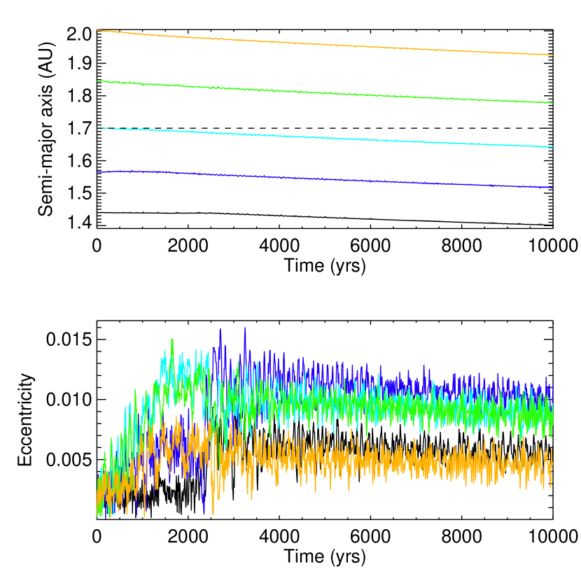
Figure 5: Orbital evolution of N=5 embryos with mass $m_{p}=3\;M_{\oplus}$ and without stochastic forces included. The dashed line shows the location of the zero-migration line.

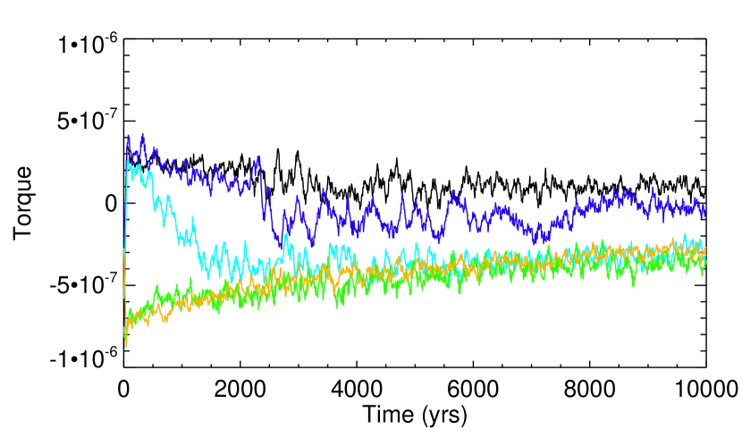
Figure 6: Time evolution of the torque experienced by the protoplanets in the case with N=5 and without stochastic forces included

Eccentricity and inclination damping resulting from the interaction with the disc are modelled by applying the following accelerations to each body:

$${\bf a}_{e}=-2\frac{({\bf v}_{p}\cdot{\bf R}_{p}){\bf R}_{p}}{R_{p}^{2}t_{e}}$$ (17)

and

$${\bf a}_{i}=-\frac{({\bf v}_{p}\cdot\hat{\bf z})}{t_{i}}\hat{\bf z}$$ (18)

where $\hat{\bf z}$ is a unit vector in the vertical direction. $t_{e}$ and $t_{i}$ are the eccentricity and inclination damping timescales for which we use the prescriptions of Cresswell & Nelson (2008):

$$t_{e}=\frac{t_{wave}}{0.78}\left[1-0.14\left(\frac{e_{p}}{h_{p}}\right)^{2}+0.06\left(\frac{e_{p}}{h_{p}}\right)^{3}+0.18\left(\frac{e_{p}}{h_{p}}\right)\left(\frac{i_{p}}{h_{p}}\right)^{2}\right]$$ (19)

and

$$t_{i}=\frac{t_{wave}}{0.544}\left[1-0.3\left(\frac{i_{p}}{h_{p}}\right)^{2}+0.24\left(\frac{i_{p}}{h_{p}}\right)^{3}+0.18\left(\frac{e_{p}}{h_{p}}\right)^{2}\left(\frac{i_{p}}{h_{p}}\right)\right]$$ (20)

where:

$$t_{wave}=\frac{M_{\star}}{m_{p}}\frac{M_{\star}}{\Sigma_{p}a_{p}^{2}}h_{p}^{4}\Omega_{p}^{-1}$$ (21)

4 Results of hydrodynamical simulations

4.1 Laminar viscous simulations

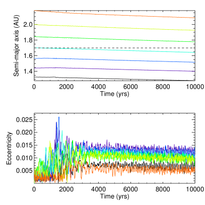
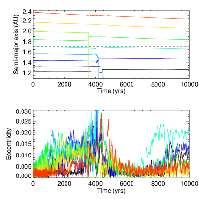
Figure 7: Left panel: Orbital evolution of N=7 embryos with mass $m_{p}=3\;M_{\oplus}$ and without stochastic forces included. Right panel: same but with N=9. The dashed line shows the location of the zero-migration line.

The orbital evolution of N=5 embryos with mass $m_{p}=3\;M_{\oplus}$ and initially separated by $4.5\;R_{mH}$ is displayed in Fig. 5. At early times, the two innermost (resp. outermost) bodies located inside (resp. outside) the opacity transition tend to undergo outward (resp. inward) migration. Regarding the third body (cyan) initially located at $R_{p}=1.7$, it tends to experience only a weak positive torque due to its close proximity to the opacity transition. Nevertheless, the strong differential migration between this body and the fourth one (green) quickly leads to the formation of a 9:8 mean motion resonance (MMR) between these two protoplanets at $t\sim 3\times 10^{2}$ yr. As revealed by Fig. 6 which displays the temporal evolution of the torques experienced by each planet, eccentricity growth due to resonant trapping makes the torque experienced by the third planet become negative, in such a way that the third and fourth planets subsequently migrate inward together while maintaining their 9:8 resonance. This arises because, just after resonant trapping, the value reached by the eccentricity of the third planet $e_{p}\sim 0.015$ is comparable to the dimensionless half-width of the planet’s horseshoe region which is estimated to be $x^{\prime}_{s}\sim 1.1a_{p}\sqrt{q/h}\sim 0.02$. Consequently, the radial excursion that the planet undergoes is eventually larger than the horseshoe region, causing thereby the (positive) corotation torque to be significantly attenuated (Bitsch & Kley 2010, Cossou et al. 2013).
These two bodies then catch up with the outward-migrating second protoplanet (blue) and enter in a 9:8 MMR with it at $t\sim 600$ yr. Again, eccentricity growth due to resonant capture causes the positive torque exerted on the second body to weaken. Although it remains positive, its amplitude is not sufficient to counterbalance the negative torques exerted on the third and fourth planets, and this three-planet system consequently suffers a slow, inward resonant migration. This proceeds until the fifth body (orange) catches up with the fourth protoplanet (green) and enters a 9:8 resonance with it at $t\sim 1000$ yr. At $t\sim 2000$ yr, the outward-migrating innermost planet (black) becomes trapped in a 9:8 MMR with the second protoplanet (blue) which, from this time onward, undergoes a marginally positive torque due to the high value reached by its eccentricity. However, as can be seen in the lower panel of Fig. 5, eccentricity pumping due to resonant interaction is relatively modest for the innermost core, with an equilibrium value of $e_{p}\sim 5\times 10^{-3}$. Consequently, the fraction of the corotation torque operating on the innermost planet is large enough for the total torque exerted on this body to remain positive, which is confirmed by looking at the evolution of the torque exerted on that planet in Fig. 6. This effect, however, is clearly not sufficient to couterbalance the negative torques experienced by the outer bodies so that at late times, the five bodies tend migrate inward in lockstep with each neighbouring pair of planets forming a 9:8 resonance. As the outer planets pass through the zero-torque radius, however, we expect the disc torques exerted on these planets to become positive so that it is likely that the swarm will ultimately stop migrating once the net torque acting on the whole system cancels (Cossou et al. 2013).

In Fig. 7 we present, the orbital evolution of simulations with N=7 (left panel) and N=9 (right panel) embryos embedded in the same disc model. We remind the reader that the embryos are initially located in such a way that bodies of the inner half migrate outward whereas bodies of the outer half migrate inward. Because they are initially located on either side of the convergence line, the fourth (cyan) and fifth (green) bodies are the first to become trapped in a 9:8 MMR. Again, eccentricity growth due to resonant trapping causes the corotation torque operating on the fourth body to be significantly attenuated so that these two planets tend to migrate inward at later times. This is exemplified in the upper panel of Fig. 8 which shows the evolution of the torque exerted on each planet as a function of time. At $t\sim 600$ yr, the third body (blue) catches up with the fourth body (cyan) and enters a 9:8 MMR with it. A general trend is that inward-migrating bodies are captured in resonance later than outward-migrating bodies. This is a direct consequence from the corotation damping effect, which tends to make the resonant swarm migrate inward, strengthening thereby the differential migration rate with the inner, outward-migrating bodies.
Once again, the evolution outcome consists of inward migration of a group of N=7 members which are in mutual mean motion resonances, with the resonance being 9:8 except for the two innermost bodies which are in 8:7 resonance. This arises because prior to resonant capture of the second body (purple) , the torque exerted on this planet is slightly stronger in comparison with that experienced by the innermost one (black), resulting in divergent migration between these two cores. Comparing Figs. 6 and 8, we see that after $\sim 10^{4}$ yr, only one planet feels a positive torque in the case where N=5 while two cores are subject to a positive torque in the simulation with N=7. This confirms the expectation that the resulting resonant system becomes more compressed as $N$ increases, and consequently more prone to dynamical instability.

Indeed, increasing the number of initial embryos to N=9 resulted in a more chaotic behaviour where protoplanets suffered close encounters and collisions, as illustrated in the right panel of Fig. 7 which displays the planets’ orbital evolution for that case. At early times, evolution proceeds similarly to that corresponding to N=7, with a system of 9 protoplanets with each body locked in a 9:8 MMR with its neighbours being formed at $t\sim 3000$ yr. From that time onward, it can be seen in the lower panel of Fig. 8, which displays the temporal evolution of the torque exerted on each planet, that the five innermost embryos located inside the convergence line undergo a positive torque whereas the others undergo a negative torque, implying a significantly compressed resonant system. At $t\sim 3500$ yr, this leads to a physical collision between the sixth (green) and seventh (light green) embryos, forming thereby a $6\;M_{\oplus}$ planet which subsequently undergoes inward migration since it is located outside the convergence line. The resulting perturbation then propagates to the inner system and causes two additional collisions at later times, between the third (dark blue) and fourth (blue) planets at $t\sim 4000$ yr and between the two innermost cores (black+purple) at $t\sim 4100$ yr. As revealed by the lower right panel of Fig. 7, these two newly formed $\sim 6\;M_{\oplus}$ planets are located inside the convergence line and have relatively modest eccentricity. This, combined with the fact that the fully-unsaturated corotation torque scales as $m_{p}^{2}$ (or equivalently as $x_{s}^{4}$) for low-mass planets, implies that these planets are subject to a stronger positive torque. Not surprisingly, the significant resulting differential migration between the outermost $6\;M_{\oplus}$ planet (blue) and its exterior inward-migrating $3\;M_{\oplus}$ neighbour (cyan) leads to capture in a 6:5 resonance at $t\sim 7000$ yr. Eccentricity growth due to resonant trapping causes the corotation torque operating on the $6\;M_{\oplus}$ to be partially attenuated, causing the two planets migrate inward together at later times while maintaining their 6:5 resonance. This process enables the innermost $6\;M_{\oplus}$ planet (black) to catch up with the outermost $6\;M_{\oplus}$ body (blue) and to enter in a 5:4 resonance with it at $t\sim 8500$ yr. Protoplanets located outside the convergence line then become trapped in MMRs with the inner ones at later times so that the evolution outcome for that case corresponds again to the formation of a stable resonant system where the two inner planets are the more massive. Since the two inner planets are trapped in resonance with sustained eccentricities, they only feel a weak positive torque despite being located interior to the convergence zone. With no strong outward push, the whole system of embryos migrates inward. The high computational cost makes it impossible to perform hydrodynamical simulations for more than $\sim 10^{4}$ yr so that the final fate of the system remains uncertain. Altough it can not be excluded that additional collisions will arise at later times, a possible issue is that the planets will reach stationary orbits once the net torque acting on the resonant system, which consists of the sum of the attenuated corotation torques and unattenuated differential Lindlbad torques exerted on each planet, cancels (Cossou et al. 2013). In Sect. 5, we will examine in more details the possible long-term evolution outcomes using N-body simulations.

In order to unveil the role of the zero-migration line on the collisions events that were observed in this simulation, we have performed a similar simulation with initially N=9 embryos but using an isothermal equation of state. In that case, all protoplanets are expected to experience inward migration due to their interaction with the gas disc. Fig. 9 shows the evolution of the planets’ semimajor-axes and eccentricities as a function of time for the isothermal run. We note that although we consider here equal-mass planets, these tend to undergo convergent migration because the surface density profile has index $\sigma<3/2$ (e.g. Pierens et al. 2011). Compared with the radiative simulation, however, the convergent migration rate is sufficiently weak in the isothermal case to prevent close encounters between embryos. This clearly demonstates that near the transition between the outward and inward migration regimes, close encounters and collisions can be stimulated due to the strong differential migration experienced by the embryos there.

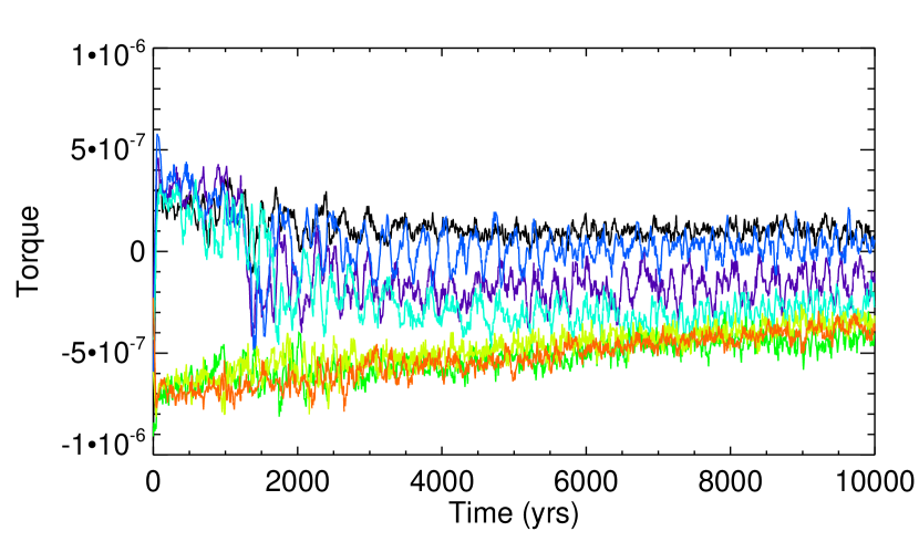
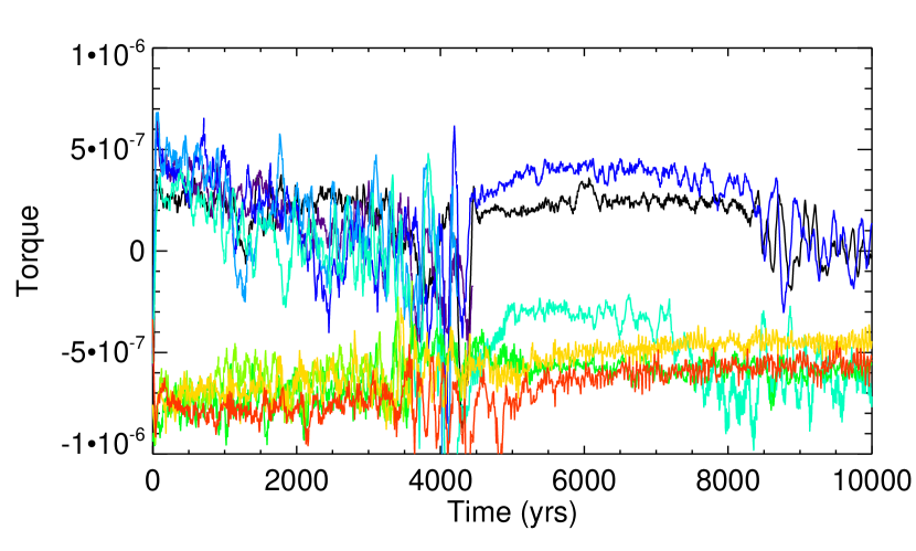
Figure 8: Upper panel:Time evolution of the torque experienced by the protoplanets in the case with N=7 and without stochastic forces included. Lower panel: same but for N=9.

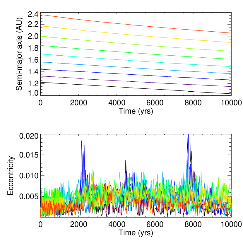
Figure 9: Time evolution of the semimajor-axes and eccentricities of protoplanets for an isothermal hydrodynamical simulation with N=9.

4.2 Effects of disc turbulence

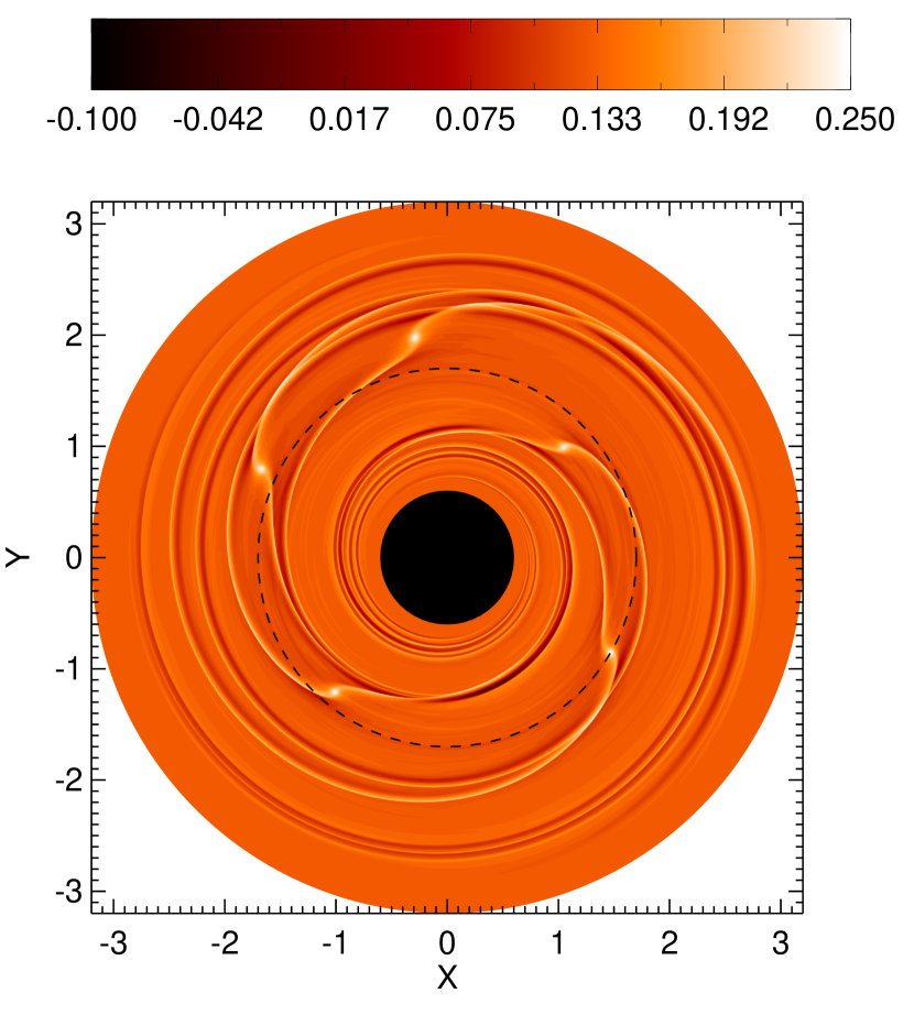
Figure 10: Snapshot of the perturbed surface density profile in the hydrodynamical simulation with initially N=5 embryos and with stochastic forces included. The dashed circle shows the location of the zero-migration line.

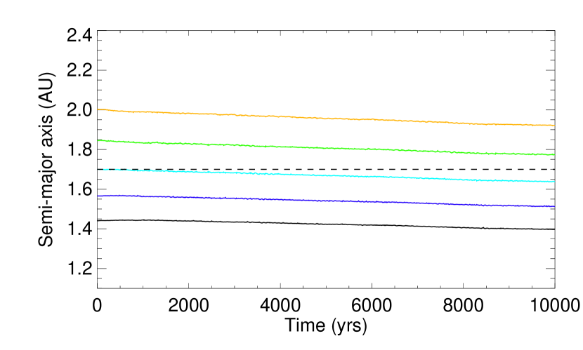
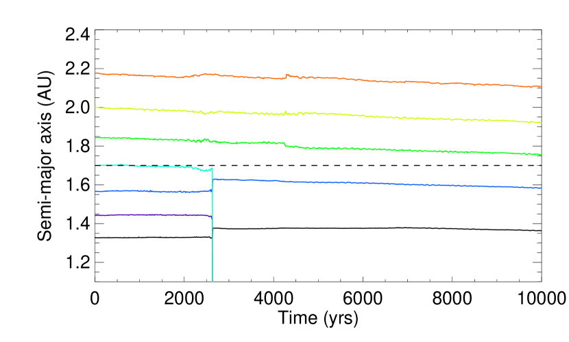
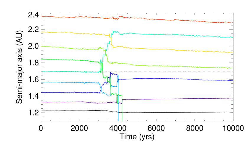
Figure 11: Top panel:: time evolution of the semimajor-axes of protoplanets in a hydrodynamical simulation with N=5 and with stochastic forces included. Middle panel: same but for N=7. Bottom panel: same but for N=9. The dashed line shows the location of the zero-migration line.

The results presented above indicate that, in the limit of a moderate initial number of objects, the formation of mean motion resonances prevents embryos from undergoing close encouters with other bodies. In this section, we examine how the stability of these resonant configurations is affected when a level of disc turbulence is accounted for. Previous work (e.g. Pierens et al. 2011) suggested that mean motion resonances are likely to be disrupted by stochastic torques in the active regions of protoplanetary discs and within disc lifetimes.
To examine this issue, we have perfomed a series of simulations for N=5,7,9 in which each body is subject to a an additional stochastic force $\@vec{F}_{\text{turb}}=-\nabla\Phi_{\text{turb}}$ where $\Phi_{\text{turb}}$ is given by Eq. 7. The temporal evolution of the planets’ semi-major axis for these three simulations is displayed in Fig.11. For N=5, Fig. 10 presents a contour plot of the perturbed surface density distribution at the beginning of the simulation. For protoplanets initially located inside the zero-migration radius, surface density perturbations inside the planets’ horseshoe regions and related to the co-orbital dynamics are clearly visible. Due to the negative entropy gradient, co-orbital dynamics leads to a positive (resp. negative) surface density pertubation ahead (resp. behind) of the planet, giving rise to a positive corotation torque. For protoplanets located outside the zero-migration line, these additional surface density perturbations are weaker, indicating a relatively faint corotation torque in that case. For this run, a sequence of 9:8 MMRs is ultimately formed so that the final fate of the system is similar to that obtained in the laminar simulation. Although these resonances are stable on average, the corresponding resonant angles are observed to oscillate between periods of circulation and libration, implying a weaker resonant locking in presence of turbulence. We notice that a similar behaviour was observed in previous studies on the capture in resonance of pairs of planets embedded in a turbulent isothermal disc (Pierens et al. 2011). This stengthens the expectation that turbulence can break resonant configurations when the typical amplitude of the stochastic density fluctuations is large enough, and consequently that the resonant systems obtained using viscous laminar disc models are more prone to destabilization in presence of turbulence. This is therefore not too surprising that collisions arise in the turbulent run with N=7, as can be seen in the middle panel of Fig. 11. Here, the resonant system that is formed at the end of the simulations is composed of two $6\;M_{\oplus}$ bodies (black+blue lines) located at the inner edge of the swarm and trapped in a 5:4 resonance plus three exterior $3\;M_{\oplus}$ protoplanets trapped in a first-order p+1:p resonance with its neighbours, where we observe a clear tendency for $p$ to increase as one moves out through the swarm.
The lower panel of Fig. 11 shows the evolution of the system for the run with N=9. Again, two $6\;M_{\oplus}$ planets (purple+blue) are formed in the course of the evolution and the final fate corresponds again to the formation of a resonant chain with the two more massive planets located in the inner half of the swarm. Although three collisions ocurred in the laminar run with N=9, it is clear, when comparing Fig. 11 with Fig. 7, that the evolution of the system is much more chaotic in the turbulent case.

4.3 Effect of the disc model

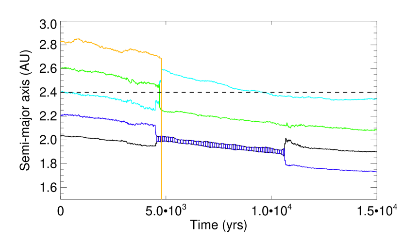
Figure 12: Time evolution of the semimajor-axes of protoplanets in a turbulent hydrodynamical simulation with initially N=5 embryos and for a disc mass equivalent to two times that of the fiducial disc model. The dashed line shows the location of the zero-migration line.

To investigate how the disc model affects the results presented above, we have performed a series of simulations using a disc model with mass twice that of the fiducial disc model, which corresponds to a the snow-line located at $\sim 4.2$ AU. Again, the initial mass of embryos is $3\;M_{\oplus}$ and their initial positions are chosen such that half of the initial population of embryos is located inside the zero-migration line, which lies at $\sim 2.4$ AU for this disc model, whereas the other half is located outside. Although not shown here, runs with stochastic forces not included show evolution outcomes consistent with those of the fiducial disc model, with growth of embryos and formation of $6\;M_{\oplus}$ protoplanets observed when the initial number of bodies is $N\geq 7$. This is not surprising since as the disc mass increases, the effect of a faster differential migration toward the zero-migration line, and which would promote close encounters between embryos, is couterbalanced by a stronger disc-induced eccentricity damping.
For runs with stochastic forces included, however, the outcomes are found to differ noticeably from those of the fiducial disc model due to more vigorous turbulent fluctuations. In that case, collisions are found to arise even for low values of the initial number of embryos, as illustrated in Fig. 12 where is displayed, for this disc model, the evolution of the planets’ semimajor-axes for N=5. Here, a $6\;M_{\oplus}$ planet (cyan) is formed at the outer edge of the swarm at $t\sim 5\times 10^{3}$ yr and is likely to become trapped at the location of the zero-torque radius at later times. From $t\sim 1.3\times 10^{4}$ yr, this planet tends to separate from the three innermost $3\;M_{\oplus}$ bodies which experience resonant inward migration with each planet forming a 8:7 resonance with its neighbours. Prior to the formation of this inner resonant system, it is interesting to note that the two innermost bodies (black+blue) entered in a coorbital 1:1 resonance and which remained stable for $\sim 5\times 10^{3}$ yr.
Again, the final fate of the system remains uncertain but it is likely that the group composed of the three innermost planets will end up on a stationary orbit once the net torque acting on this three-planet system will cancel out (Cossou et al. 2013)

5 Results of N-body runs

In Sect. 3, we have presented how analytical formulae for the Type I torques can be calibrated using the results of hydrodynamical simulations. Here, we present the main results that emerge from $\sim 600$ N-body runs of protoplanets embedded in a radiative protoplanetary disc that we have performed using the prescriptions we obtained for Type I migration. The aims of this alternative approach are to i) study the long-term evolution of a swarm of protoplanets migrating toward the convergence line and ii) examine the statistical properties of the planetary systems which are formed through this process.

5.1 Comparison with hydrodynamical simulations

5.1.1 Runs without stochastic forces included

We first describe the range of outcomes that are observed in simulations with initial conditions chosen as close as possible to those for the hydrodynamical simulations presented in Sect. 4. We performed 100 N-body simulations for situations with N=7 and N=9 initial embryos. These simulations did not include stochastic forcing and differed only in the initial azimuthal positions of the embryos. For N=7, collisions occured in 53% of the simulations. Objects as large as 9 $M_{\oplus}$ formed in 6% of the simulations. In the runs with N=9, virtually all (95%) of the simulations included collisions, as expected from the hydrodynamical simulations presented in Sect. 4. Most (77%) simulations only produced 6 $M_{\oplus}$ planets, but a significant number (17%) formed 9 $M_{\oplus}$ planets and one simulation formed a 12 $M_{\oplus}$ core.

The left panel of Fig. 13 displays the evolution as a function of time of the planets’ orbital positions and masses for a run representative of the range of the observed outcomes. Overall, the early stages of evolution are consistent with what is seen in the corresponding hydrodynamical simulation, involving outward (resp. inward) migration of the innermost (resp. outermost) bodies plus formation of two $6\;M_{\oplus}$ protoplanets inside the zero-migration line by $\sim 10^{4}$ years. It is interesting to notice that of these two $6\;M_{\oplus}$, one is formed at $\sim 8\times 10^{3}$ years through the merging of two co-orbital planets that entered in a 1:1 resonance at $\sim 2\times 10^{3}$ years. An additional $6\;M_{\oplus}$ body is produced at $t\sim 1.8\times 10^{4}$ yr as a result of the collision between two $3\;M_{\oplus}$ objects. After $\sim 3\times 10^{4}$ years, the systems attains a quasi-stationary state and consists of three $6\;M_{\oplus}$ objects plus two $3\;M_{\oplus}$ bodies trapped in a resonant chain and evolving on non-migrating orbits. Moving from inward to outward, the resonances which are formed are 5:4, 7:6, 7:6, 8:7 and 6:5. This stationary configuration is reached when the positive torque exerted on the two innermost $6\;M_{\oplus}$ bodies (blue and black lines in Fig. 13) counterbalances the torques experienced by the three other bodies, leading to a zero net torque acting on the whole system (Cossou et al. 2013).

5.1.2 Effect of stochastic forces

To illustrate the dependence of the results presented above on the presence of disc turbulence, we have performed a set of simulations but with stochastic forces acting on the protoplanets included. We remind the reader that hydrodynamical simulations in which stochastic forces are included (see Sect. 4.2) indicated that collisions are more likely to occur in that case due to the general tendency for turbulent fluctuations to break resonant configurations. In agreement with this result, we find that collisions occured in $97\;\%$ of the N-body runs performed with N=7 and in $100\%$ of the simulations performed with N=9. Therefore, it is not surprising to observe a clear trend for forming more massive embryos when stochastic forces are included. For example, $36\;\%$ of the runs with N=7 resulted in the production of $9\;M_{\oplus}$ bodies whereas this number increases to $50\;\%$ for N=9. In this latter case, two simulations resulted in the formation of $12\;M_{\oplus}$ protoplanets. Moreover, we note that we performed a series of turbulent runs with initial separations of $6\;R_{mH}$, and which resulted in the production of $9\;M_{\oplus}$ cores in $30$ of a total of $100$ simulations, which suggests that these statistics are relatively robust with regards to the value for the initial separation of embryos.
The right panel of Fig. 13 illustrates the evolutionary outcome for a simulation in which two $12\;M_{\oplus}$ planets are produced. At $t\sim 10^{5}$ yr, a non-migrating compact system is formed with two co-orbital planets of $3\;M_{\oplus}$ and $6\;M_{\oplus}$ located at the inner edge of the swarm and in a 7:6 resonance with an exterior $3\;M_{\oplus}$ protoplanet. At $t\sim 1.2\times 10^{5}$ years, the formation of a $12\;M_{\oplus}$ body through the collision of two exterior $6\;M_{\oplus}$ bodies (yellow+red) destabilizes the inner part of the swarm, which subsequently leads to the merging of the three inner planets into an additional $12\;M_{\oplus}$ embryo. From this time, the system is composed of two $12\;M_{\oplus}$ bodies plus an exterior $3\;M_{\oplus}$ embryo which evolves on a quasi-circular orbit at the nominal convergence line. The two $12\>M_{\oplus}$ planets enter in a 6:5 resonance at later times and resonantly migrate inward until they reach the inner edge of the disc. This configuration remained stable until the end of the simulation which was evolved for $5\times 10^{5}$ yr. We note that although these planets evolve inside the zero-migration line, they experience a negative torque from the disc because the (positive) corotation torque is saturated for such a planet mass (see Sect. 3).

5.2 Effect of changing the initial mass distribution and statistical overview

In order to examine the dependence of our results on the initial mass distribution, we performed two additional sets of $100$ simulations using a randomised mass distribution. In the first series of runs, the mass of each embryo is sampled from a Gaussian distribution with mean $\mu_{m}=3\;M_{\oplus}$ and standard deviation $\sigma_{m}=1\;M_{\oplus}$, while in the second set of simulations, we set $\mu_{m}=1\;M_{\oplus}$ and $\sigma_{m}=0.5\;M_{\oplus}$. The total mass of embryos is chosen to be $30\;M_{\oplus}$ in both cases. Moreover, we choose the orbital position of the inner planet to be uniformely distributed between $1.1\leq a_{p}\leq 1.2$ AU whereas the initial separations of other planets are set to $nR_{mH}$, where $4\leq n\leq 5$ is randomly chosen according to a uniform distribution.
Fig. 14 shows the distribution of mass of the most massive planet which is formed in these two series of simulations. In the case where $\mu_{m}=3\;M_{\oplus}$ and $\sigma_{m}=1\;M_{\oplus}$ (left panel), we see that $\sim 7\;M_{\oplus}$ embryos are most common but of the $100$ simulations, a significant number of them ($43\%$) resulted in the formation of protoplanets with masses in the range $8\leq m_{p}\leq 10\;M_{\oplus}$ within $5\times 10^{5}$ yr. This is in good agreement with the results of simulations with initially equal-mass embryos presented in Sect. 5.1.2. Giant planet cores with masses $\geq 10\;M_{\oplus}$ were produced in $8\;\%$ of the simulations.
In the case where $\mu_{m}=1\;M_{\oplus}$ and $\sigma_{m}=0.5\;M_{\oplus}$ (right panel), $14\;\%$ of runs resulted in the formation of bodies with masses in the range $8\leq m_{p}\leq 10\;M_{\oplus}$, with only one run leading to the formation of a core with mass $\geq 10\;M_{\oplus}$. We believe this is related to the fact that the initial population of embryos with initial masses $\lesssim 1\;M_{\oplus}$ experience corotation torque saturation (see Sect. 3). Consequently, they undergo inward Type I migration even these are located inside the opacity transition, which tends to substantially reduce the process of convergent migration at the planet trap.
These results indicate that forming giant planet cores at the zero-torque radius is likely to occur provided it involves massive impacts between bodies of a few Earth masses which do not experience corotation torque saturation and which formed earlier through an alternative process.

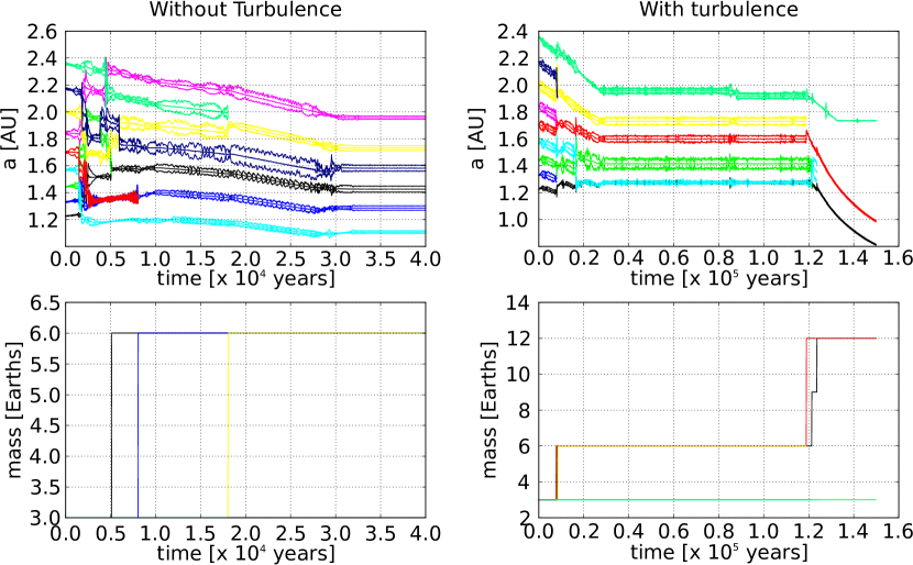
Figure 13: Left: time evolution of protoplanets’ orbital positions (top panel) and masses (lower panel) for a N-body run with intially N=9 embryos and without stochastic forces included. Right: same but with stochastic forces included.

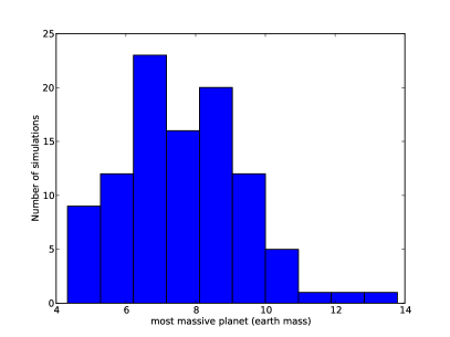
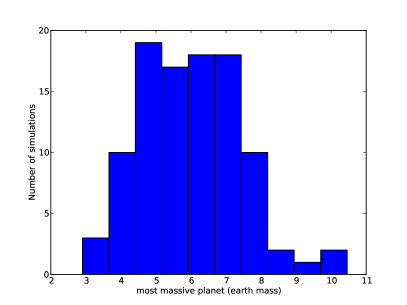
Figure 14: Left panel: distribution of mass of the most massive planet which is formed in N-body runs with stochastic forces included and in which the mass of each embryo is sampled from a Gaussian distribution with $\mu_{m}=3\;M_{\oplus}$ and $\sigma_{m}=1\;M_{\oplus}$. Right panel: same but for $\mu_{m}=1\;M_{\oplus}$ and $\sigma_{m}=0.5\;M_{\oplus}$.

6 Discussion

In this section, we discuss how the location of the opacity transition we considered here depends on the disc model that is adopted and examine under which conditions collisional planetary growth at this opacity transition is expected to arise.
In order to determine the location of the opacity transition, we balance radiative losses with viscous heating, which gives:

$$2\sigma T_{\text{eff}}^{4}=\frac{9}{4}\nu\Sigma\Omega^{2}$$ (22)

For an optically thick disc, we remind that the midplane temperature $T$ is related to the effective temperature $T_{eff}$ by (see Eq. 4):

$$T^{4}=\frac{3}{8}\tau T_{\text{eff}}^{4}$$ (23)

Given that $\tau=\kappa\Sigma/2$, Eq. 22 can be recast as:

$$\sigma T^{4}=\frac{27}{128}\nu\kappa\Sigma^{2}\Omega^{2}$$ (24)

Moreover, in the context of the standard $\alpha$ prescription of Shakura & Sunyaev (1973) , the effective kinematic viscosity is given by $\nu=\alpha c_{s}H$, where $c_{s}=(\gamma_{ad}{\cal R}T/\mu)^{1/2}$ (${\cal R}$ and $\mu$ are the gas constant and the mean molecular weight respectively) is the sound speed and $H=c_{s}/\Omega$ the disc scale height. Evaluating the previous equation at the opacity transition gives the following expression for the location of the transition radius $R_{t}$:

$$\frac{R_{t}}{R_{0}}=\left(\frac{27}{128}\frac{\gamma_{ad}{\cal R}}{\mu\sigma}\frac{\kappa_{t}\Sigma_{0}^{2}\Omega_{0}}{T_{t}^{3}}\alpha\right)^{1/(2\sigma+3/2)}$$ (25)

where $T_{t}$ and $\kappa_{t}$ denote the values for the temperature and opacity at the transition respectively. Here, we have used the fact that $\Sigma=\Sigma_{0}(R/R_{0})^{-\sigma}$ and $\Omega=\Omega_{0}(R/R_{0})^{-3/2}$, where $\Omega_{0}$ is the angular velocity at $R=R_{0}$.
Furthermore, convergent migration at the opacity transition for bodies of a few Earth masses arises provided that the corotation torque remains unsaturated. We expect the corotation torque to remain close to its fully unsaturated value provided that (e.g. Baruteau & Masset 2013):

$$t_{\text{U-turn}}\leq t_{\text{dif}}\leq t_{\text{lib}}/2$$ (26)

For given values of $\alpha$ and the mass ratio $q=m_{p}/M_{\star}$, this condition provides an estimation of the range of radii for which the corotation torque is fully unsaturated. We find:

$$0.52\left(\frac{\Omega_{0}R_{0}}{c_{s,t}}\right)^{2}q^{6/7}\alpha^{-4/7}\leq\frac{R}{R_{0}}\leq 0.025\left(\frac{\Omega_{0}R_{0}}{c_{s,t}}\right)^{2}q^{2/3}\alpha^{-4/9}$$ (27)

where $c_{s,t}$ is the value of the sound speed at the opacity transition. In the top panel of Fig. 15 we plot the location of $R_{t}$ as a function of the $\alpha$ viscous stress parameter and for the disc model that we employed in the simulations. The region located in between the dashed and solid-dashed lines in Fig. 15 corresponds to that where the corotation torque remains unsaturated for a $3\;M_{\oplus}$ planet, and which is defined by Eq. 27. Therefore, the intersection between the solid line and the shaded area in Fig. 15 represents the range of radii where convergent migration of $3\;M_{\oplus}$ protoplanets can occur. For this disc model, this process is expected to arise in the region from $\sim 1.5$ to $\sim 2.2$ AU, in good agreement with the location of the zero-torque radius in our hydrodynamical and N-body simulations.
For a given value of $\alpha$, Eq. 25 predicts that the location of the opacity transition will increase with $\Sigma$. However, looking at the upper panel of Fig. 15, it is clear that as $\Sigma$ increases, the range of $\alpha$ values for which the corotation torque remains unsaturated is shifted toward lower values. In the context of the formation of the giant planets in the Solar System, this implies that both a significantly massive disc and a relatively low value for $\alpha$ will be needed for the convergent migration mechanism to operate in the Jupiter-Saturn region. This is illustrated in the lower panel of Fig. 15 which shows that for a disc model with $\sigma=1.5$, convergent migration at $\sim 4$ AU arises provided that the disc mass corresponds to ten times the MMSN. Of course, these results will strongly depend on the opacity transition that is considered. We nevertheless expect a similar mechanism to occur at any opacity transition interior to which the temperature gradient is steep enough to allow for outward migration of Earth-mass bodies. Testing other opacity transitions is beyond the scope of that paper but we will discuss in a future paper the influence of changing the opacity table. Finally, we notice that formation of giant planet cores through collisions of Earth-mass bodies may also be possible at other kinds of planet traps like those arising at a dead zone or at the radius where stellar heating begins to take over viscous heating (Hasegawa & Pudritz 2011).

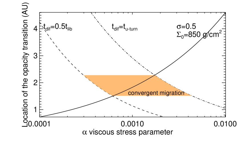
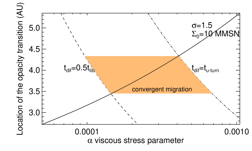
Figure 15: Top panel: Location of the opacity transition (solid line) as a function of the value for the $\alpha$ viscous stress parameter and for our fiducial disc model. The dashed line shows the location where the viscous timescale $t_{dif}$ becomes equal to half of the horseshoe libration timescale ($t_{lib}$) whereas the solid-dashed line shows the radius where $t_{dif}$ equals the U-turn timescale. The intersection between the shaded area and the solid line corresponds to the range of radii where convergent migration for $3\;M_{\oplus}$ bodies is expected to occur. Lower panel: same but for a disc model ten times more massive than the MMSN.

7 Conclusion

We have presented the results of both hydrodynamical and N-body simulations of the evolution of a swarm of Earth-mass protoplanets that gravitationally interact near a zero-migration line. The embryos are initially located around an opacity transition which plays the role of a planet trap where the Type I torque cancels. For bodies with masses in the range $1-10\;M_{\oplus}$ and evolving inside the opacity transition, Type I migration proceeds outward whereas it is directed inward if these are located further out. The main aim of this work is to examine the possible outcomes that arise when low-mass protoplanets convergently migrate toward a zero-migration radius and in particular whether giant planet cores can be formed at such places through giant impacts between embryos of a few Earth masses.
Hydrodynamical simulations show that equal-mass embryos with mass of $3\;M_{\oplus}$ located on both sides of a convergence zone tend to enter in a resonant chain whose stability depends on the initial number of objects and whether or not planets experience stochastic forces due to turbulence. For a limited number of bodies and in the absence of stochastic forcing, a sequence of resonances appears to be stable so that close encounters betweeen embryos are prevented. Increasing the initial number of protoplanets however leads to a significant compression of the system and eventually to the destabilization of these resonant chains. Formation of $6\;M_{\oplus}$ protoplanets from $3\;M_{\oplus}$ embryos is observed to occur in that case on a timescale $\leq 10^{4}$ yr.
Not surprisingly, including a moderate level of turbulence corresponding to a value for the $\alpha$ viscous stress parameter of $\alpha\sim 2\times 10^{-3}$ clearly enhances this process of collisional planetary growth. Interestingly, we find that a significant fraction ($\sim 50\;\%$) of the N-body runs with stochastic forces included and performed with masses randomly sampled from a Gaussian distribution with $\mu_{m}=3\;M_{\oplus}$ resulted in the formation of giant planet cores with mass $\geq 8-10\;M_{\oplus}$ in $\sim 5\times 10^{5}$ yr. For a randomised mass distribution with $\mu_{m}=1\;M_{\oplus}$, however, only $\sim 15\;\%$ of the N-body runs produced giant planet cores. We conclude that forming giant planet cores at convergence zones is efficient provided that it involves collisions between embryos with mass $\gtrsim 2\;M_{\oplus}$ and which formed earlier according to the classical runaway/oligarchic growth scenario (Levison et al. 2010) or through accretion of cm-sized pebbles (Morbidelli & Nesvorny 2012).
For a protoplanetary disc with mass typical of the MMSN, we find that the mechanism presented here may allow the in-situ formation of giant planet cores from Earth-mass bodies at $\sim 2$ AU whereas very massive discs ($\geq 10$ times the MMSN) are required to form $\sim 10\;M_{\oplus}$ bodies at $4-5$ AU. We note however that we considered here a zero-migration line corresponding to a particular change in the opacity regime. Other planet traps located further than $\sim 4$ AU are expected to arise in typical protoplanetary disc models. For example, the transition where stellar irradiation begins to provide most of the heating of the disc gives rise to an additional planet trap located at $2-40$ AU, depending on the mass accretion rate (Hasegawa & Pudritz 2011). Planet traps can also exist at locations where the thermal diffusion timescale becomes longer than the horseshoe libration timescale, leading to a saturation of the corotation torque in the outer regions. Since the horseshoe libration timescale depends on the planet mass, planets with different masses tend to converge toward different radii. We will focus on the role of these additional planet traps on the formation of giant planet cores in a future publication.
The N-body runs that we have presented are the simplest we can perform. One limitation of our work is that the embryos do not accrete planetesimals or pebbles as they migrate. If there is a sufficient supply of pebbles, accretion may be very rapid for embryos of $\sim 1\;M_{\oplus}$ (Lambrechts & Johansen 2012; Morbidelli & Nesvorny 2012), with the consequence that embryo masses may change significantly over the timescales of the simulations. Morevover, the position of the zero-migration line remains fixed in the course of the simulations. In a more realistic scenario, we expect the convergence zone to move inward as the disc disperses (Lyra et al 2010; Horn et al 2012). We will present in a forthcoming paper the results of both hydrodynamical and N-body simulations that account for the inward migration of the zero-torque radius due to photoevaporation and irradiation from the central star effects.