Damped Ly$\alpha$ Absorption Systems in Semi-Analytic Models with Multiphase Gas

Abstract

We investigate the properties of damped Ly$\alpha$ absorption systems (DLAs) in semi-analytic models of galaxy formation, including new modeling of the partitioning of cold gas into atomic, molecular, and ionized phases, and a star formation recipe based on the density of molecular gas. We use three approaches for partitioning gas into atomic and molecular constituents: a pressure-based recipe and metallicity-based recipes with fixed and varying UV radiation fields. We identify DLAs by adopting an assumed gas density profile for galactic discs and passing lines of sight through our simulations to compute ${\rm H}_{\rm I}$  column densities. We find that models with “standard” gas radial profiles — computed assuming that the average specific angular momentum of the gas disc is equal to that of the host dark matter halo — fail to reproduce the observed column density distribution of DLAs, regardless of the assumed gas partitioning. These models also fail to reproduce the distribution of velocity widths $\Delta v$ of low-ionization state metal systems, overproducing low $\Delta v$ relative to high $\Delta v$ systems. Models with “extended” radial gas profiles — corresponding to gas discs with higher specific angular momentum, or gas in an alternate extended configuration — are able to reproduce quite well the column density distribution of absorbers over the column density range $19<\log~{}\mbox{${N}_{\rm HI}$}\ <22.5$ in the redshift range $2<z<3.5$. The model with pressure-based gas partitioning and the metallicity-based recipe with a varying UV radiation field also reproduce the observed line density of DLAs, ${\rm H}_{\rm I}$  gas density, and $\Delta v$ distribution at $z<3$ well. However all of the models investigated here underproduce DLAs and the ${\rm H}_{\rm I}$  gas density at $z>3$. This may indicate that DLAs at high redshift arise from a different physical phenomenon, such as outflows or filaments. If this is the case, the flatness in the number of DLAs and ${\rm H}_{\rm I}$  gas density over the redshift interval $0<z<5$ may be due to a cosmic coincidence where the majority of DLAs at $z>3$ arise from intergalactic gas in filaments or streams while those at $z<3$ arise predominantly in galactic discs. We further investigate the dependence of DLA metallicity on redshift and $\Delta v$ in our favored models, and find good agreement with the observations, particularly when we include the effects of metallicity gradients.

1 Introduction

The study of gas in absorption against background quasars (quasar absorption systems) has a long and rich observational history (Wolfe et al., 1986, 1995; Storrie-Lombardi et al., 1996; Storrie-Lombardi & Wolfe, 2000; Péroux et al., 2003). Damped Lyman-$\alpha$ systems (DLAs), defined as systems with column density ${\rm log}~{}\mbox{${N}_{\rm HI}$}\ >20.3$ ${\rm atoms~{}cm}^{-2}$, are of particular interest for studies of galaxy formation because they are believed to arise predominantly from neutral gas within or closely associated with galaxies. DLAs are believed to contain the majority of neutral gas in the Universe (Storrie-Lombardi & Wolfe, 2000; Wolfe & Prochaska, 2000; Péroux et al., 2003; Prochaska et al., 2005; Noterdaeme et al., 2009) and are therefore reservoirs for future star formation. Indeed, absorption studies are currently the only means of probing the ${\rm H}_{\rm I}$ content of galaxies at significant redshifts and provide an orthogonal means of studying galaxy evolution. Observational properties that can be measured for DLAs include their number density and column density distribution, metallicities, and kinematic properties (Lanzetta et al., 1995; Storrie-Lombardi et al., 1996; Pettini et al., 1994, 1997; Prochaska & Wolfe, 1997, 2000). These observations provide important constraints on the gas content of galaxies at high redshift, and indirectly constrain how gas is converted into stars, and how gas and metals are cycled into and out of galaxies in inflows and outflows. These, in turn, provide key constraints on some of the most uncertain aspects of our models of galaxy formation.

There has been a significant amount of observational activity and progress in this area in recent years. Large surveys such as the Sloan Digital Sky Survey (SDSS Schneider et al., 2010) and BOSS (Eisenstein et al., 2011) have provided extensive target samples of optically detected quasars, yielding greatly improved statistics for samples of high redshift absorbers ($1.5\lower 2.15277pt\hbox{$\;\buildrel<\over{\sim}\;$}z\lower 2.15277pt\hbox{$\;\buildrel<\over{\sim}\;$}4.5$). These improved statistics have greatly tightened the constraints on the shape of the column density distribution function, comoving line density of DLAs, and the evolution of the cosmological neutral gas density (e.g. Noterdaeme et al., 2012). Font-Ribera et al. (2012) employed a cross-correlation analysis of DLAs from the BOSS survey with the Ly$\alpha$ forest and were able to obtain constraints on the DLA cross-section as a function of halo mass. Rafelski et al. (2012) and Neeleman et al. (2013)have published metallicities for a large number of DLAs in the redshift interval $2<z<4$, providing constraints on the build-up of heavy elements in the cold gas phase of galaxies across cosmic time. In addition, the UV-sensitive Cosmic Origins Spectrograph (COS) on the Hubble Space Telescope (HST) is now enabling studies of DLAs at lower redshift $z\lower 2.15277pt\hbox{$\;\buildrel<\over{\sim}\;$}1$, which may be more easily connected with populations detected in emission and with the present day galaxy population (Meiring et al., 2011; Battisti et al., 2012). Recent studies with COS have also yielded a wealth of information on ionized gas within low-redshift haloes (e.g. Tumlinson et al., 2011).

Two different pictures for the origin and nature of DLAs have been debated in the literature. Based on the observed kinematics of low-ionization metal systems in DLAs, Wolfe et al. (1986) and Prochaska & Wolfe (1997, hereafter PW97) presented a picture in which thick, extended disc galaxies give rise to DLAs, yet explaining how a sufficient number of large disc galaxies could have formed by $z\sim 3$ remains a challenge. In contrast, in the context of the hierarchical picture arising in a Cold Dark Matter (CDM) cosmogony, many DLAs would be expected to be associated with smaller, lower mass systems (e.g. Haehnelt et al., 1998). However, reproducing the distribution of DLA kinematics has remained a significant challenge for hierarchical models (Maller et al., 2001; Razoumov et al., 2008; Pontzen et al., 2008). These two scenarios have very different implications for galaxy evolution — the former requires large disc galaxies to be in place by $z\sim 3$, and the latter has implications for the expected star formation rates, stellar masses, and kinematics of DLAs and their counterparts.

A number of previous theoretical studies have made specific predictions for the properties of DLAs in the framework of the CDM paradigm (e.g., Kauffmann & Charlot, 1994; Kauffmann, 1996; Gardner et al., 1997; Haehnelt et al., 1998; Maller et al., 2001, 2003; Nagamine et al., 2004b, a, 2007; Pontzen et al., 2008; Fumagalli et al., 2011; Altay et al., 2011; Cen, 2012; van de Voort et al., 2012; Kulkarni et al., 2013; Altay et al., 2013). Early numerical hydrodynamic simulations typically neglected feedback from stellar and supernova-driven winds, or contained weak forms of stellar feedback. These simulations had moderate success in reproducing the column density distribution, cosmological neutral gas density, and line density of DLAs at high redshift ($1\lower 2.15277pt\hbox{$\;\buildrel<\over{\sim}\;$}z\lower 2.15277pt\hbox{$\;\buildrel<\over{\sim}\;$}4$), although they had difficulty reproducing the turnover in the column density distribution at ${\rm log}~{}\mbox{${N}_{\rm HI}$}\ \sim 22$ ${\rm atoms~{}cm}^{-2}$ (Nagamine et al., 2004a). These simulations were not able to discriminate between different phases of gas, and it was speculated that the turnover could be due to the ${\rm H}_{\rm I}$-H₂ transition. However, recent observational results from the BOSS survey (Font-Ribera et al., 2012) have shown that while these high column density systems are rare, they do exist, relaxing some of this tension, although the origin of the turnover still remains something of a puzzle (Erkal et al., 2012). Many of these simulations had relatively small volumes and modeled the DLA column density distribution by characterizing the relationship between DLA cross-section and dark matter (DM) halo mass, then convolving this relationship with a DM halo mass function from larger volume dissipationless simulations.

More recent simulations found that the inclusion of more effective stellar feedback and winds had a significant effect on the predicted DM halo mass to DLA cross section relationship. For example, Nagamine et al. (2007) found that in simulations with strong winds, galaxies in low mass haloes ejected much of their gas, resulting in a lower DLA cross section, thus shifting the DLA population into higher mass host haloes. Qualitatively similar results have been found by Pontzen et al. (2008), Fumagalli et al. (2011), and Cen (2012), although the detailed slope, normalization, and redshift dependence of the predicted halo mass to DLA cross section relationship are different in these different simulations. Recently, Cen (2012) particularly emphasized the importance of outflows for reproducing the observed properties of DLAs including their kinematics.

CDM-based models have also had difficulty reproducing the observed metallicities of DLAs (Somerville et al., 2001; Maller et al., 2001; Nagamine et al., 2004b, 2005; Pontzen et al., 2008; Fumagalli et al., 2011). They have consistently predicted higher average metallicities, and none have reproduced the tail to very low metallicity, although again, simulations with strong stellar feedback and winds have been more successful. Cen (2012) find that a significant number of $z\lower 2.15277pt\hbox{$\;\buildrel>\over{\sim}\;$}3$ DLAs originiate in intergalactic gas. A combination of these intergalactic DLAs and the ejection of metals by galactic winds lowers the average metallicities, bringing them into better agreement with observations.

Semi-analytic models (SAMs), based within the framework of the CDM paradigm for structure formation (Blumenthal et al., 1984), have been widely used to produce a general picture of how density fluctuations in the primordial universe evolve into the observable galaxy population (Percival et al., 2002; Tegmark et al., 2004; Eisenstein et al., 2005). Rather than solving detailed equations of hydrodynamics and thermodynamics for individual particles or grid cells, SAMs use simple but physically motivated “recipes” to track bulk quantities such as the total mass in stars, hot gas, cold gas, metals, etc, in various “zones” (e.g. within a galaxy, within a dark matter halo, in a halo infall region, or in the intergalactic medium). In some cases, SAMs attempt to track these quantities in radial bins within a galactic disc (Kauffmann, 1996; Avila-Reese et al., 2001; Dutton & van den Bosch, 2009; Fu et al., 2010; Kauffmann et al., 2012). Although they cannot offer the detailed spatial and kinematic information provided by fully numerical hydrodynamical simulations, SAMs do have a number of advantages over these techniques. Numerical hydro simulations of galaxy formation still must rely heavily on “sub-grid” recipes for important processes such as star formation and stellar feedback. These are treated in a similar manner in SAMs, but the effect of varying the details of these recipes and their parameters can be explored much more thoroughly because of their greater computational efficiency. SAMs can provide “mock catalogs” for very large numbers of galaxies, comparable to modern surveys, while this is still inaccessable for numerical hydro simulations. Finally, we still do not understand many of the details of the physics that shapes galaxy formation. It is easier to explore, albeit qualitatively, somewhat more schematic solutions in SAMs, which may point the way towards more physically rigorous investigations with numerical techniques.

SAMs have been used extensively to investigate and interpret observations of nearby and distant galaxies in emission. A recent generation of SAMs that incorporates feedback from accreting black holes has been shown to be successful at reproducing a broad range of observations. These include the stellar mass function and luminosity function, gas fraction vs. stellar mass relation, and relative fraction of early vs. late type galaxies as a function of stellar mass at $z=0$, and the evolution of the global stellar mass density and star formation rate density with redshift from $z\sim 6$ to 0 (Bower et al., 2006; Croton et al., 2006; De Lucia & Blaizot, 2007; Monaco et al., 2007; Somerville et al., 2008b; Hopkins et al., 2009b; Guo et al., 2010; Somerville et al., 2012). However, these models still fail to reproduce some important observations. For example, they predict that low mass galaxies form too early and are too quiescent at late times, reflecting star formation histories that apparently do not match observational constraints (Fontanot et al., 2009; Weinmann et al., 2012). Numerical hydrodynamical simulations with similar implementation of “sub-grid” recipes largely show the same successes and problems (Weinmann et al., 2012). It has been suggested (e.g. Fontanot et al., 2009; Krumholz & Dekel, 2012) that inadequacies in our modeling of star formation and/or stellar feedback are likely culprits for these remaining difficulties in reproducing observations of low-mass galaxies.

Meanwhile, recent observational and theoretical work has greatly advanced our understanding of the physics that regulates star formation on galactic scales. The vast majority of previous cosmological simulations relied on the classical “Kennicutt-Schmidt” (KS) relation as a recipe for describing how cool gas turns into stars. The KS relation, based on observations of nearby spiral galaxies and starburst nuclei, says that the star formation rate surface density ($\Sigma_{SFR}$) is proportional to the total gas surface density ($\Sigma_{H}=\Sigma_{HI}+\Sigma_{H_{2}}$) (Schmidt, 1959; Kennicutt, 1989, 1998). The KS relation is frequently approximated as a power law, $\Sigma_{SFR}\propto\Sigma_{H}^{N}$, with $N\sim 1.4$, above a critical total gas surface density $\Sigma_{\rm crit}$. Empirical studies have shown that $\Sigma_{\rm crit}\simeq 3$–10  ${\rm M}_{\odot}{\rm pc}^{-2}$(Martin & Kennicutt, 2001).

However, Wong & Blitz (2002) showed that $\Sigma_{SFR}$ is more tightly correlated with the density of molecular hydrogen $\Sigma_{H_{2}}$ (as traced by CO) than with the total gas density. These results were confirmed and expanded upon with the results from the THINGS survey (Walter et al., 2008) combined with CO maps from BIMA SONG and HERACLES (Helfer et al., 2003; Leroy et al., 2009). These studies showed that $\Sigma_{SFR}\propto\Sigma_{H_{2}}^{N}$ with $N$ very close to unity, implying that star formation takes place in molecular gas with roughly constant efficiency (Bigiel et al., 2008a, 2011). These results underlined the importance of modeling the partitioning of gas into atomic and molecular phases in theoretical models of galaxy formation.

Blitz & Rosolowsky (2004, 2006) showed that, empirically, the fraction of molecular to molecular plus atomic gas, $f_{H_{2}}$, in nearby spirals is tightly correlated with the disc midplane pressure. Ostriker et al. (2010) proposed a theoretical explanation for this relationship, arguing that the thermal pressure in the diffuse Interstellar Medium (ISM), which is proportional to the UV heating rate and therefore to the SFR, adjusts until it balances the midplane hydrostatic pressure set by the vertical gravitational field. Other recent theoretical work has argued that, as H₂ forms most efficiently on dust grains, the metallicity of the gas, along with its surface density, should be an important factor in determining $f_{H_{2}}$ (Krumholz et al., 2008, 2009a; Gnedin & Kravtsov, 2010). Using high resolution numerical simulations of isolated galaxies with detailed chemistry and an H₂-based star formation recipe, Robertson & Kravtsov (2008) showed that $f_{H_{2}}$ depended on metallicity, gas surface density, and the UV background radiation. Gnedin & Kravtsov (2010, 2011) characterized this dependence in detail with high resolution numerical cosmological simulations with detailed chemistry. The impact on the structural properties of disc galaxies of using an H₂-based star formation recipe rather than a traditional KS recipe has recently been explored with high resolution “zoom-in” cosmological simulations (Christensen et al., 2012).

Several SAM-based studies have modelled the partitioning of gas into atomic and molecular phases using various approaches, and studied the effect of using an H₂-based star formation recipe. Obreschkow et al. (2009) partitioned gas into atomic and molecular components using the empirical pressure-based relation of Blitz & Rosolowsky (2006, hereafter BR) in post-processing on the Millennium semi-analytic models. Lagos et al. (2011) and Fu et al. (2010) implemented gas partitioning self-consistently into SAMs using two approaches: the empirical pressure-based recipe of BR, and the theoretically motivated metallicity-dependent recipe of Krumholz et al. (2009b, hereafter KMT09). These models then implemented an H₂-based star formation recipe based on their computed H₂ fractions. Using a similar approach, Somerville, Popping & Trager (in prep; SPT14) explored the partitioning of gas using the BR recipe, the KMT recipe, and an additional metallicity dependent recipe provided by Gnedin & Kravtsov (GK), along with an H₂-based star formation recipe based on the Bigiel et al. (2008a) observational results. They concluded that the GK recipe was more successful and robust, particularly at low metallicities, than the KMT formulation (see also Krumholz & Gnedin, 2011). Popping et al. (2014, hereafter PST14) presented the predictions of these models for the gas content of galaxies in ${\rm H}_{\rm I}$, H₂, and CO from redshift six to zero for direct comparison with upcoming surveys of gas tracers in emission.

The SAM developed by SPT14 does not predict the internal structure of galaxies in detail, so we assume that the density profiles of the gas and stellar discs are described by a smooth exponential function in both the vertical and radial dimensions. We rely on simplified approximations to estimate the scale length of the gas disc from the specific angular momentum (spin) of the host dark matter halo. This approach has been shown to reproduce the evolution of stellar disc sizes (as traced by their optical light) from $z\sim 2$ to 0 (Somerville et al., 2008c), and also reproduces the observed sizes of ${\rm H}_{\rm I}$ discs in the nearby universe, the observed sizes of CO discs in local and high redshift galaxies for the small sample currently available, and the spatial extent of the SFR density in nearby and high-redshift galaxies (PST14). However, we also consider models in which the gas is more extended than in our standard models, either because the gas that forms the disc or is accreted onto the disc has higher specific angular momentum than the dark matter halo (as some numerical simulations suggest; e.g. Robertson et al., 2004, 2006a; Agertz et al., 2011; Guedes et al., 2011), accreted gas from cold streams deposit their angular momentum to the inner parts of the halo (Kimm & Cen, 2013), or the gas is in a non-rotationally supported extended configuration such as tidal tails or an outflow (Stewart et al., 2011, 2013).

In this paper, we make use of the SAMs developed in SPT14 and PST14 to explore for the first time the predictions for the properties of DLAs in semi-analytic models with partitioning of gas into different phases and an H₂-based star formation recipe. We investigate the impact of the gas partitioning, star formation recipe, and assumptions about the structure of the cold gaseous disc on the main observable properties of DLAs and confront our predictions with the latest observations. The paper is organized as follows. In section 2, we describe the “base-line” semi-analytic models, the new recipes for partitioning gas into an atomic and molecular component, and the new H₂-based star formation recipes. We also describe our methodology for generating gas distributions, and how we compile mock catalogs of DLAs. In section 3, we present our predictions for key DLA observables, including the DLA column density distribution as a function of redshift, DLA cross-section as a function of halo mass and redshift, comoving density of DLAs and cosmological neutral gas density as a function of redshift, distribution of DLA velocity widths, DLA metallicity distribution, and DLA metallicity as a function of velocity width and redshift. We discuss the implications of our results in section 4, and summarize and conclude in section 5. Throughout this paper, we adopt the following values for the cosmological parameters: $\Omega_{\rm m}=0.28$, $\Omega_{\Lambda}=0.72$, $H_{0}=70.0$, $\sigma_{8}=0.81$, and $n_{s}=0.96$. Our adopted baryon fraction is 0.1658. These values are consistent with the seven-year Wilkinson Microwave Anisotropy Probe (WMAP) results (Komatsu et al., 2011). All quoted metallicities are relative to solar.

2 Models and Methodology

2.1 The Semi-Analytic Model of Galaxy Formation

The semi-analytic models (SAMs) used here to compute the formation and evolution of galaxies within a $\Lambda$CDM cosmology were originally presented in Somerville & Primack (1999) and Somerville et al. (2001), with significant changes described in detail in Somerville et al. (2008b, hereafter S08), Somerville et al. (2012, hereafter S12), and most recently in SPT14. The S12 SAM includes the following physically motivated ingredients: (1) the growth of dark matter structure in a hierarchical clustering framework as described by ‘merger trees’, (2) shock heating and radiative cooling of gas, (3) conversion of cold gas into stars via an empirical ‘Kennicutt-Schmidt’ relation, (4) evolution of stellar populations, (5) a combination of feedback and metal enrichment of the interstellar and intracluster medium from supernovae, (6) ‘quasar’ and ‘radio’ mode black hole growth and feedback from AGN, (7) starbursts and morphological transformation due to galaxy mergers. Here, we briefly summarize these ingredients — for a more detailed description of the model framework, see S08 and S12. The ingredients in the models used here are the same as those described in S12, with the exception of the new recipes for gas partitioning and star formation, which we describe below. Throughout this work, we assume a standard $\Lambda$CDM universe and a Chabrier stellar initial mass function (IMF; Chabrier, 2003).

The merging histories (or merger trees) of dark matter haloes are constructed based on the Extended Press-Schechter formalism using the method described in Somerville & Kolatt (1999), with improvements described in S08. These merger trees record the growth of dark matter haloes via merging and accretion, with each “branch” representing a merger of two or more haloes. We follow each branch back in time to a minimum progenitor mass $M_{\rm res}$. We refer to $M_{\rm res}$ as the mass resolution of our simulation where we have adopted $M_{\rm res}=10^{9.5}\mbox{${\rm M}_{\odot}$}$ in all the models presented here. Our SAMs give nearly identical results when run on the EPS merger trees or on merger trees extracted from dissipationless N-body simulations (Lu et al., 2013, ; Porter et al. in prep).

Whenever dark matter haloes merge, the central galaxy of the largest progenitor becomes the new central galaxy, and all others become ‘satellites’. Satellite galaxies lose angular momentum due to dynamical friction as they orbit and may eventually merge with the central galaxy. To estimate this merger timescale we use a variant of the Chandrasekhar formula from Boylan-Kolchin et al. (2008). Tidal stripping and destruction of satellites are also included as described in S08. We have checked that the resulting mass function and radial distribution of satellites (sub-haloes) agrees with the results of high-resolution N-body simulations that explicitly follow sub-structure (Macciò et al., 2010).

Before reionization, each halo contains a mass of hot gas equal to the univeral baryon fraction times the virial mass of the halo. After reionization, which we assume to be complete by $z=11$, the photoionizing background suppresses the collapse of gas into low-mass haloes. We use the results of Gnedin (2000) and Gnedin et al. (2004) to model the fraction of baryons that can collapse as a function of halo mass after reionization.

When a dark matter halo collapses or experiences a merger that more than doubles the mass of the largest progenitor, the hot gas is shock-heated to the virial temperature of the new halo. This gas then cools and collapses based on a simple spherically symmetric model. We assume that cold gas is accreted only by the central galaxy, even though realistically, satellite galaxies should receive some fraction of the new cold gas.

All newly cooling gas collapses to form a rotationally supported disc. The scale radius is based on the initial angular momentum of the gas and the halo profile, assuming angular momentum is conserved and the self-gravity of the collapsing baryons causes contraction in the inner part of the halo (Blumenthal et al., 1986; Flores et al., 1993; Mo et al., 1998). Somerville et al. (2008c) showed that this approach reproduced the observed size versus stellar mass relation for discs from $z\sim 0$ to $2$. In this scenario, the cold gas specific angular momentum is set equal to that of the dark matter: $f_{j}=j_{\rm gas}/j_{DM}=1$.

Star formation occurs in two modes, a “normal” mode in isolated discs, and a merger-driven “starburst” mode. Star formation in the “normal” mode is modelled as described in Section 2.3 below. The efficiency and timescale of the merger driven burst mode is a function of the merger mass ratio and the gas fractions of the progenitors, and is based on the results of hydrodynamic simulations of binary galaxy mergers (Robertson et al., 2006b; Hopkins et al., 2009a).

Some of the energy from supernovae and massive stars is assumed to be deposited in the ISM, resulting in the driving of a large-scale outflow of cold gas from the galaxy. The mass outflow rate is parameterized as a function of the galaxy circular velocity times the star formation rate, as motivated by the “energy driven” wind scenario.

Some fraction of this ejected gas escapes from the potential of the dark matter halo, while some is deposited in the hot gas reservoir within the halo, where it becomes eligible to cool again. The fraction of gas that is ejected from the disc but retained in the halo versus ejected from the disc and halo is a function of the halo circular velocity (see S08 for details), such that low-mass haloes lose a larger fraction of their gas. The gas that is ejected from the halo is kept in a larger “reservoir”, along with the gas that has been prevented from falling in due to the photoionizing background. This gas is allowed to “re-accrete” onto the halo as described in S08.

Each generation of stars also produces heavy elements, and chemical enrichment is modelled in a simple manner using the instantaneous recycling approximation. For each parcel of new stars ${\rm d}m_{*}$, we also create a mass of metals ${\rm d}M_{Z}=y\,{\rm d}m_{*}$, which we assume to be instantaneously mixed with the cold gas in the disc. The yield $y$ is assumed to be constant, and is treated as a free parameter. When gas is removed from the disc by supernova driven winds as described above, a corresponding proportion of metals is also removed and deposited either in the hot gas or outside the halo, following the same proportions as the ejected gas.

Mergers are assumed to remove angular momentum from the disc stars and to build up a spheriod. The efficiency of disc destruction and spheroid growth is a function of progenitor gas fraction and merger mass ratio, and is parameterized based on hydrodynamic simulations of disc-disc mergers (Hopkins et al., 2009a). These simulations indicate that more “major” (closer to equal mass ratio) and more gas-poor mergers are more efficient at removing angular momentum, destroying discs, and building spheroids. Note that the treatment of spheroid formation in mergers used here has been updated relative to S08 as described in Hopkins et al. (2009b). The updated model produces good agreement with the observed fraction of disc vs. spheroid dominated galaxies as a function of stellar mass (Hopkins et al., 2009b, Porter et al. in prep).

In addition, mergers drive gas into galactic nuclei, fueling black hole growth. Every galaxy is born with a small “seed” black hole (typically $\sim 100\,\mbox{${\rm M}_{\odot}$}$ in our standard models). Following a merger, any pre-existing black holes are assumed to merge fairly quickly, and the resulting hole grows at its Eddington rate until the energy being deposited into the ISM in the central region of the galaxy is sufficient to significantly offset and eventually halt accretion via a pressure-driven outflow. This results in self-regulated accretion that leaves behind black holes that naturally obey the observed correlation between BH mass and spheroid mass or velocity dispersion (Di Matteo et al., 2005; Robertson et al., 2006a; Somerville et al., 2008b).

There is a second mode of black hole growth, termed “radio mode”, that is thought to be associated with powerful jets observed at radio frequencies. In contrast to the merger-triggered mode of BH growth described above (sometimes called “bright mode” or “quasar mode”), in which the BH accretion is fueled by cold gas in the nucleus, here, hot halo gas is assumed to be accreted according to the Bondi-Hoyle approximation (Bondi, 1952). This leads to accretion rates that are typically only about $\la 10^{-3}$ times the Eddington rate, so that most of the BH’s mass is acquired during episodes of “bright mode” accretion. However, the radio jets are assumed to couple very efficiently with the hot halo gas, and to provide a heating term that can partially or completely offset cooling during the “hot flow” mode (we assume that the jets cannot couple efficiently to the cold, dense gas in the infall-limited or cold flow regime).

2.2 Multiphase Gas Partitioning

Throughout this paper we refer rather loosely to “cold” gas, which is gas that according to our simple cooling model has been able to cool below $10^{4}$ K via radiative atomic cooling. Most previous cosmological simulations have considered all of this “cold” gas to be eligible to form stars. Here, we partition it into components that we label atomic, molecular, and ionized, and only allow the “molecular” component to participate in star formation. As we do not explicitly track the temperature or density of the “cold” gas in our models, this is obviously still extremely schematic. However, when we refer to “cold” gas, we are referring to gas that is in one of these three states and is dynamically associated with the galactic disc (rather than in an extended hot halo, an outflow, etc).

At each timestep, we compute the scale radius of the cold gas disc using the angular momentum based approach described above, and assume that the total (${\rm H}_{\rm I}$+ ${\rm H}_{2}$) cold gas distribution is described by an exponential with scale radius $r_{\rm gas}$. We do not attempt to track the scale radius of the stellar disc separately, but make the simple assumption that $r_{\rm gas}=\chi_{\rm gas}r_{\rm star}$, with $\chi_{\rm gas}=1.7$ fixed to match stellar scale lengths at $z=0$. Bigiel & Blitz (2012) showed that this is a fairly good representation, on average, for the discs of nearby spirals. We then divide the gas disc into radial annuli and compute the fraction of molecular gas, $f_{\rm H_{2}}(r)\equiv\Sigma_{\rm H_{2}}(r)/[\Sigma_{\rm H_{2}}(r)+\Sigma_{\rm HI}(r)]$, in each annulus, as described below.

2.2.1 Ionized Gas

Most (if not all) previous semi-analytic models have neglected the ionized gas associated with galaxies, which may be ionized either by an external background or by the radiation field from stars within the galaxy. Here we include a simple analytic estimate of the ionized gas fraction motivated by the model presented in Gnedin (2012). We assume that some fraction of the total cold gas in the galaxy, $f_{\rm ion,int}$, is ionized by the galaxy’s own stars. In addition, a slab of gas on each side of the disc is ionized by the external background radiation field. Gas is assumed to be ionized if it lies below a critical threshold surface density $\Sigma_{\rm HII}$. Throughout this paper we assume $f_{\rm ion,int}=0.2$ (as in the Milky Way) and $\Sigma_{\rm HII}=0.4\,\mbox{${\rm M}_{\odot}{\rm pc}^{-2}$}$ (as in Gnedin 2012). Applying this model within our SAM gives remarkably good agreement with the ionized fractions as a function of circular velocity shown in Fig. 2 of Gnedin (2012), obtained from hydrodynamic simulations with time dependent and spatially variable 3D radiative transfer of ionizing radiation from local sources and the cosmic background.

2.2.2 Molecular Gas: Pressure Based Partioning

We consider two approaches for computing the molecular gas fractions in galaxies. The first is based on the empirical pressure-based recipe presented by Blitz & Rosolowsky (2006, BR) who found that the molecular fraction $R_{\rm mol}\equiv\Sigma_{\rm H2}/\Sigma_{\rm HI}$ is correlated with the disc hydrostatic mid-plane pressure $P$:

$$R_{\rm mol}=\left(\frac{P}{P_{0}}\right)^{\alpha_{\rm BR}}$$ (1)

where $P_{0}$ and $\alpha_{\rm BR}$ are free parameters that are obtained from a fit to the observational data. We adopted $\log P_{0}/k_{B}=4.23$ cm³ K and $\alpha_{\rm BR}=0.8$ from Leroy et al. (2008).

We estimate the hydrostatic pressure as a function of the distance from the center of the disc $r$ as (Elmegreen, 1989, 1993; Fu et al., 2010):

$$P(r)=\frac{\pi}{2}G\Sigma_{\rm gas}(r)[\Sigma_{\rm gas}(r)+f_{\sigma}(r)\Sigma_{*}(r)]$$ (2)

where $G$ is the gravitational constant, $\Sigma_{\rm gas}$ is the cold gas surface density, $\Sigma_{*}$ is the stellar surface density, and $f_{\sigma}$ is the ratio of the vertical velocity dispersions of the gas and stars:

$$f_{\sigma}(r)=\frac{\sigma_{\rm gas}}{\sigma_{*}}$$ (3)

Following Fu et al. (2010), we adopt $f_{\sigma}(r)=0.1\sqrt{\Sigma_{*,0}/\Sigma_{*}}$, where $\Sigma_{*,0}\equiv m_{*}/(2\pi r_{*}^{2})$, based on empirical scalings for nearby disc galaxies.

2.2.3 Molecular Gas: Metallicity Based Partioning

Gnedin & Kravtsov (2011) performed high-resolution “zoom-in” cosmological simulations with the Adaptive Refinement Tree (ART) code of Kravtsov & et al. (1999), including gravity, hydrodynamics, non-equilibrium chemistry, and simplified radiative transfer. These simulations are able to follow the formation of molecular hydrogen through primordial channels and on dust grains, as well as dissociation of molecular hydrogen and self- and dust- shielding. These simulations also include an empirical ${\rm H}_{2}$-based star formation recipe.

Gnedin & Kravtsov (2011) presented a fitting function based on their simulations, which effectively parameterizes the fraction of molecular hydrogen as a function of the dust-to-gas ratio relative to the Milky Way, $D_{\rm MW}$, the UV radiation field relative to the Milky Way value $U_{\rm MW}$, and the neutral gas surface density $\Sigma_{HI+H_{2}}$. Following Gnedin & Kravtsov (2010), we take the dust-to-gas ratio to be equal to the metallicity of the cold gas in solar units, $D_{\rm MW}=Z/Z_{\odot}$. The UV background is defined as the ratio of the interstellar FUV flux at $1000{\mathrm{\AA}}$, relative to the Milky Way value of $10^{6}$ photons cm^-2 s^-1 sr^-1 eV^-1 (Draine, 1978; Mathis et al., 1983), $U_{\rm MW}$. In this work, we create two sets of models: one where the UV background is fixed to the Milky Way value ($U_{\rm MW}=1$) (Murray & Rahman, 2010; Robitaille & Whitney, 2010) , and one where it is equal to the global star formation rate within the galaxy, $U_{\rm MW}=$ SFR M_⊙ yr^-1.

The fitting functions from Gnedin & Kravtsov (2010) are intended to characterize the formation of ${\rm H}_{2}$ on dust grains, which is the dominant mechanism once the gas is enriched to more than a few tenths of Solar metallicity. However, other channels for ${\rm H}_{2}$ formation in primordial gas must be responsible for producing the molecular hydrogen out of which the first stars formed. Studies with numerical hydrodynamic simulations containing detailed chemical networks and analytic calculations have shown that ${\rm H}_{2}$ can form through primordial channels in dark matter haloes once they grow above a critical mass of $M_{\rm III}\sim 10^{5}\,\mbox{${\rm M}_{\odot}$}$ (e.g. Nakamura & Umemura, 2001; Glover, 2013). This gas can then form “Pop III” stars which pollute their surroundings and enrich the ISM to $Z_{\rm III}\sim 10^{-3}Z_{\odot}$ (Schneider et al., 2002; Greif et al., 2010; Wise et al., 2012). Since these processes are thought to have taken place in haloes that are much smaller than our resolution limit, we represent them in a simple manner. We adopt a “floor” to the molecular hydrogen fraction in our haloes, $f_{\rm H2,floor}$. In addition, we “pre-enrich” the initial hot gas in haloes, and the gas that is accreted onto haloes due to cosmological infall, to a metallicity of $Z_{\rm pre-enrich}$. We adopt typical values of $f_{\rm H2,floor}=10^{-4}$ and $Z_{\rm pre-enrich}\sim 10^{-3}\,\mbox{${\rm Z}_{\odot}$}$, based on the numerical simulation results mentioned above (Haiman et al., 1996; Bromm & Larson, 2004). Our results are not sensitive to reasonable changes in these values, as shown in SPT14.

2.3 Star Formation

The “classical” Kennicutt-Schmidt (KS) recipe (Kennicutt, 1998) assumes that the surface density of star formation in a galaxy is a function of the total surface density of the cold neutral gas (atomic and molecular), above some threshold surface density $\Sigma_{\rm crit}$. This approach has been used to model star formation in most previous SAMs and numerical hydrodynamical simulations. Here, we instead use a star formation recipe based on the ${\rm H}_{2}$ content of the galaxy, motivated by recent observational results.

Bigiel et al. (2008a) found, based on observations of spiral galaxies from the THINGS survey, that the star formation timescale in molecular gas is approximately constant, i.e.

$$\Sigma_{\rm SFR}=A_{\rm SF}\,{\Sigma_{\rm H_{2}}}^{N_{\rm SF}}$$ (4)

with $N_{\rm SF}\simeq 1$.

Observations of higher density environments, such as starbursts and high redshift galaxies, suggest that above a critical $H_{2}$ surface density, the star formation timescale becomes a function of $\Sigma_{\rm H_{2}}$ such that the star formation law steepens. Recent work in which a variable conversion factor between CO and $H_{2}$ is accounted for suggests that $N_{\rm SF}\simeq 2$ for high $\Sigma_{\rm H_{2}}$ (Narayanan et al., 2012b). This steepening is also expected on theoretical grounds (Krumholz et al., 2009b; Ostriker & Shetty, 2011). Therefore, in SPT14 we also considered an ${\rm H}_{2}$-based star formation recipe of the form

$$\Sigma_{\rm SFR}=A_{\rm SF}\,\left(\Sigma_{\rm H_{2}}/(10\mbox{${\rm M}_{\odot}$}{\rm pc}^{-2})\left(1+\frac{\Sigma_{H_{2}}}{\Sigma_{\rm H_{2},crit}}\right)^{N_{\rm SF}}\right)$$ (5)

In SPT14, we found that the “two-slope” star formation recipe produces better agreement with observations of star formation rates and stellar masses in high redshift galaxies, so we adopt it in all of the models presented in this work. For the parameter values, we adopt $A_{\rm SF}=6.0\times 10^{-3}\,\mbox{${\rm M}_{\odot}$}~{}{\rm yr}^{-1}~{}{\rm kpc}^{-2}$, $\Sigma_{\rm H_{2},crit}=70\mbox{${\rm M}_{\odot}$}$ pc^-2, and $N_{\rm SF}=1.0$, consistent with the observational results discussed above.

2.4 Model Variants

We consider nine main variants of our models: three recipes for gas partitioning (the pressure-based BR recipe and the metallicity-based GK recipe with a fixed/variable UV radiation field), and three choices for the specific angular momentum of the gas relative to the dark matter halo, parameterized by $f_{j}$. We consider fixed values of $f_{j}=1$ and $f_{j}=2.5$, and also a set of models in which $f_{j}$ is set based on the merger history of the galaxy. The $f_{j}=2.5$ models result in stellar and gaseous disks with higher specific angular momentum than their dark matter halos, and are motivated by numerical simulations that suggest this situation may arise due to stellar driven winds and/or cold flows (see Section 1 and 4.1 for a more detailed discussion and references). In the merger models, we compute the disc properties and star formation rates using the $f_{j}=1$ models, then place the gas in a more extended distribution based on the halo’s merger history, as we discuss further below. These model variants are denoted GKfj1, GKj1, BRj1, GKfj25, GKj25, BRj25, GKfjm, GKjm, and BRjm and are summarized in Table 1. While we only model azimuthally symmetric extended cold gas discs, we consider them as a proxy for other processes thay may cause the gas to be more extended.

Although we use the same ${\rm H}_{2}$-based star formation recipe in all of our models, both the choice of $f_{j}$ and the gas partitioning recipe can affect the star formation efficiency. A larger value of $f_{j}$ leads to larger discs and lower gas densities overall, less efficient formation of ${\rm H}_{2}$ and less efficient star formation. Similarly, the different gas partitioning recipes lead to different ${\rm H}_{2}$ fractions as a function of mass and redshift (see PST14) and therefore again to higher or lower star formation efficiency, since only ${\rm H}_{2}$ can form stars in our models.

Table 1: Model Definitions

Model	f${}_{H_{2}}$	UMW	f${}_{j}=j_{\rm gas}/j_{\rm DM}$
GKfj1	GK	1	1.0
GKj1	GK	$\propto$SFR	1.0
BRj1	BR	-	1.0
GKfj25	GK	1	2.5
GKj25	GK	$\propto$SFR	2.5
BRj25	BR	-	2.5
GKfjm∗	GK	1	1.0, 1.5, 2.5
GKjm∗	GK	$\propto$SFR	1.0, 1.5, 2.5
BRjm∗	BR	-	1.0, 1.5, 2.5

${}^{*}~{}f_{j}=1.0,~{}1.5,~{}2.5$ depending on if the galaxy has undergone no mergers, only minor mergers, or at least one major merger respectively.

Our merger-based models are very crude and used to investigate the impact of mergers on the angular momentum of the gas discs. In these merger models, we begin with the BRj1 and GKj1 models respectively. In post-processing, we boost the $f_{j}$ value to 1.5 or 2.5 after the galaxy has had a minor or major merger, respectively. These models reflect the idea that some of the orbital angular momentum of the merging galaxy may be transferred to internal (spin) angular momentum following a merger. This effect has been observed in numerical simulations (e.g. Robertson et al., 2006a; Robertson & Kravtsov, 2008; Sharma et al., 2012), which suggest that major mergers have a larger effect on the specific angular momentum distribution. Our $f_{j}$ values in these models contain a small, but arbitrary offset, comparable to their results. One important inconsistency in the merger models is that by increasing the cold gas angular momentum, we decrease the cold gas density, which in turn will decrease the star formation rate. Since $f_{j}$ is increased after running the semi-analytic model, the stellar masses and star formation rates reflect those of the $f_{j}=1$ models and are artificially high. For these reasons, we treat the ‘merger’ models more as toy models that provide some information on the different effects of the distribution of cold gas on DLA properties; however, we focus the majority of our analysis on the four other models.

The semi-analytic models contain a number of free parameters. These are kept fixed to the same values used in S12, except those involved in the star formation recipes, which are specified above. These parameter values were found to reproduce fundamental galaxy properties at $z=0$. As shown in SPT14 and 3.1, the updated star formation recipes have a very minor effect on the model results used for calibration, such as stellar mass function and gas mass functions.

2.5 Selecting HI absorption systems

We obtain a catalog of host haloes by extracting haloes along lightcones from the Bolshoi simulations (Klypin et al., 2011; Behroozi et al., 2010). These lightcones cover a 1 by 1 deg² area on the sky over a redshift range $0<z<5$ and contain galaxies with dark matter halo masses from $10^{9.5}$ to $\sim 10^{14.5}$ M_⊙. However, the Bolshoi simulation begins to become incomplete at $V_{vir}\simeq 50$ km s^-1, $M_{h}\simeq 10^{10}\mbox{${\rm M}_{\odot}$}$; see Klypin et al. (2011) for more details. These haloes are then populated with galaxies as described above.

The molecular and atomic hydrogen gas is distributed in a disc with an exponential radial and vertical profile. The vertical scale height is proportional to the radial scale length, $z_{g}=\chi_{z}r_{g}$, where $\chi_{z}=0.4$ is a constant, in agreement with observations of moderate redshift galaxies (Bruce et al., 2012). We explore different values of $\chi_{z}$, although reasonable values of $\chi_{z}$ (i.e. not razor-thin discs) have a minimal effect on our results.

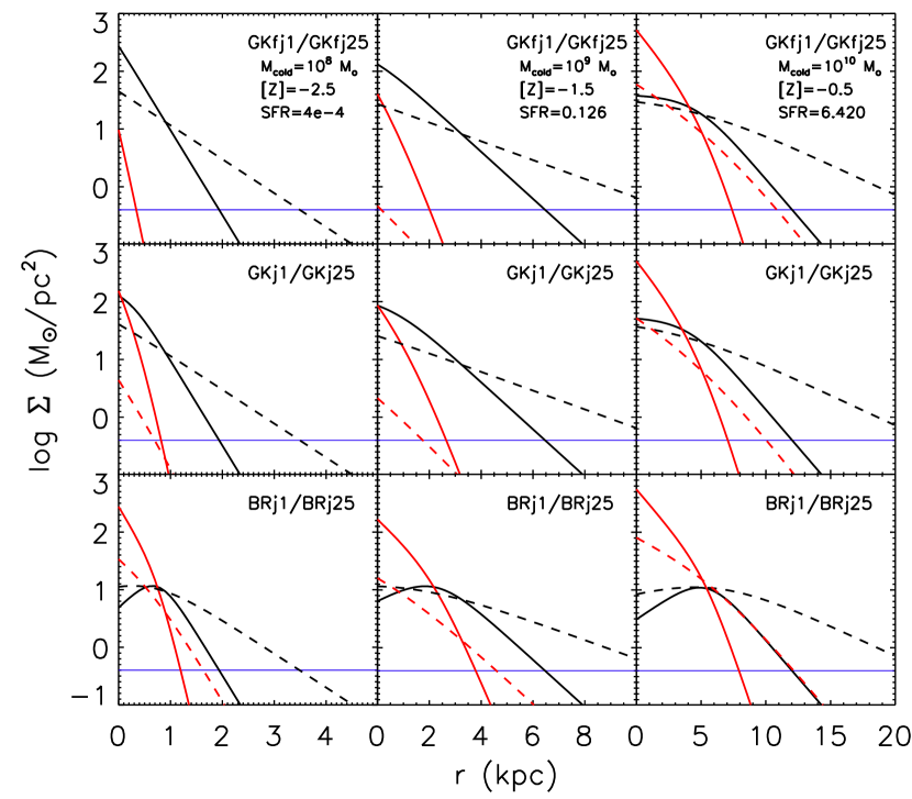
Figure 1: Cold gas radial profiles for three typical galaxies in the $f_{j}=1$ (solid line) and $f_{j}=2.5$ (dashed line) models with redshifts $2<z<3$. The HI gas (black), H₂ (red), and HII (blue) surface densities are shown. Cold gas mass and metallicity increase from left to right from ${\rm log}~{}Z=-2.5$ to $-0.5$ and ${\rm log}~{}M_{\rm cold}/\mbox{${\rm M}_{\odot}$}=8$ to 10. The top row shows the GKf models, the middle row the GK models, and the bottom row the BR models. Since stars form based on the density of H₂ (red), this illustrates that the $f_{j}=1$ models are more efficient at forming stars than the $f_{j}=2.5$ models. Moreover, star formation is much more efficient in low mass halos in the BR and GK models than the GKf models (note the lack of any H₂ in the lowest mass galaxy in the GKfj25 model). However, the star formation efficiency becomes similar in all three models at high masses and metallicities.

The central gas density is then defined as $n_{0}=M_{\rm cg}/(4\pi\mu m_{H}r^{2}_{g}z_{g})$, where $M_{\rm cg}$ is the atomic and molecular gas, $m_{H}$ is the mass of the hydrogen atom, and $\mu$ is the mean molecular weight of the gas. The atomic gas density as a function of radius along and height above the plane is given by

$$n_{\rm HI}(r,z)=n_{0}\Bigl{(}1-f_{H_{2}}(r)\Bigr{)}\exp\Bigl{(}-\frac{r}{r_{g}}\Bigr{)}\exp\Bigl{(}-\frac{|z|}{z_{g}}\Bigr{)}$$ (6)

In Figure 1 we show gas profiles for three galaxies with cold gas masses of ${\rm log}~{}M_{\rm cold}/\mbox{${\rm M}_{\odot}$}=8,~{}9,~{}10$ and metallicities ${\rm log}~{}Z/\mbox{${\rm Z}_{\odot}$}=-2.5,~{}-1.5,~{}-0.5$ at $2<z<3$ for the f_j = 1 and 2.5 models in the SAMs (as seen face-on). Each row shows the difference in cold gas partitioning for our three models and three fiducial galaxies. Star formation is much more efficient in low mass halos in the BR and GK models than the GKf models due to the high cold gas density threshold for H₂ formation in the latter. However once a significant amount of metals have been produced, the star formation efficiency converges in all three models as can be seen in galaxies with high masses and metallicities. For reference, a neutral hydrogen column density of $N_{HI}=2\times 10^{20}$ cm^-2 corresponds to a gas surface density of $\Sigma_{HI}=10$ M_⊙ pc^-2. Figure 1 demonstrates the impact on the gas distribution of the different assumptions for gas partitioning, star formation, and gas angular momentum.

The models provide the radial distance from the central galaxy for each satellite galaxy, and we assign a random azimuth and polar angle $\phi$ and $\theta$ for each satellite’s position with respect to the central. With the positions determined for every galaxy in each lightcone, we generate 20,000 random sightlines and integrate the three-dimensional gas density distribution along the sightline. Each galaxy is given a random orientation angle with respect to the sightline. All sightlines as well as the properties of all haloes with observed column densities above a threshold of $\mbox{${N}_{\rm HI}$}>10^{19}~{}\mbox{${\rm atoms~{}cm}^{-2}$}$ are then saved as our catalog of absorption systems.

We then generate low-ionization line profiles by assuming the gas is distributed in small clouds within the disc, using a similar approach to that of Maller et al. (2001). The relevant parameters are: $\sigma_{\rm int}$, the internal velocity dispersion of each cloud; $N_{c}$, the number of clouds; and $\sigma_{\rm cc}$, their isotropic random motions. Following PW97, we take $\sigma_{\rm int}=4.3$ km s^-1. PW97 derived this value from Voigt profile fits to their observations with $N_{c}=5$ being the minimum acceptable number of components. Increasing the number of clouds to as high as 60 did not improve the goodness of fit for a disc model since the model discs are relatively thin. Following Maller et al. (2001), we assume the gas discs are cold and set $\sigma_{\rm cc}=10$ km s^-1. We combine these internal velocities with the rotational velocity of the disc as well as the relative orbital velocity of the satellite galaxy with respect to the central (when applicable). For each sightline, we treat the gas density distribution as a continuous probability distribution for the positions of the clouds (Maller et al., 2001). We then generate low ionization line profiles by randomly distributing 20 clouds with the same optical depth along the line of sight. Finally, we ‘measure’ the velocity width, $\Delta v_{90}$, by taking the difference between the pixel containing 5% and 95% of the total optical depth.

In generating the low-ionization line profiles, we make a number of simplifying assumptions. Satellite galaxies are assumed to be on circular orbits. Gas discs are assumed to have a simple radial profile in addition to being axisymmetric. The gas distribution is independent of galaxy environment or Hubble type. We do not account for distortion in gas discs due to the gravitational effects of other galaxies or effects due to previous merger events, except very crudely in the merger (“m”) models as described above.

3 Results

In this section, we compare the predictions for our suite of models with a set of observations of DLAs. To calibrate our models, in section 3.1 we present the $z=0$ stellar, HI, and ${\rm H}_{2}$ mass functions for our models along with observations from local galaxies. In section 3.2 - 3.4, we present column density distribution functions, the comoving line density of DLAs, the cosmological neutral gas density in DLAs ($\Omega_{DLA}$), and DLA cross sections and halo masses as a function of redshift for all of our models and high-redshift DLAs. The DLA metallicity distribution, the cosmic evolution of DLA metallicities, the effects of metallicity gradients, and DLA kinematics are presented in sections 3.5 and 3.6. In sections 3.5 and 3.6, we only consider the $f_{j}=1$ and 2.5 models as the merger-based models have very similar metallicities to the $f_{j}=1$ models. Additionally, we feel that our merger-based models are too crude to meaningfully attempt to predict the kinematics. We focus the majority of our analysis on the GKj25 and BRj25 models, since the $f_{j}=1$ models fail to reproduce the column density distribution, the number of DLAs, and the mass of HI in DLAS (although the $f_{j}=1$ models are actually the closest to the ‘fiducial’ model presented in previous SAMs, e.g. S08 and S12). The GKfj25 model produces a large number of low mass “pristine” halos, which experience no star formation and so contain gas close to the pre-enriched metallicity, which we believe to be unphysical. Note that in this paper, we focus on the observational properties of the DLAs themselves. In a follow-up paper, we will present the optical properties of the DLA host galaxies in our models (Berry et al. 2014, in prep.).

3.1 Local Stellar and Cold Gas Mass Functions

The usual approach used in semi-analytic models is to calibrate the models using a subset of observations of $z\sim 0$ galaxies. The galaxy stellar mass function and cold gas fractions, or mass functions of cold gas, are commonly used quantities for this calibration procedure. A more extensive comparison with observations for the GKfj1, GKj1, and BRj1 models is presented in SPT14 and PST14. In addition, the BRj1 model produces extremely similar predictions to the models presented in S08 and S12. Here we examine the impact of varying the H₂ formation recipe and the distribution of cold gas ($f_{j}$) on several fundamental calibration quantities: the local galaxy stellar mass function (GSMF), HI mass function (HIMF), and H₂ mass function (H2MF).

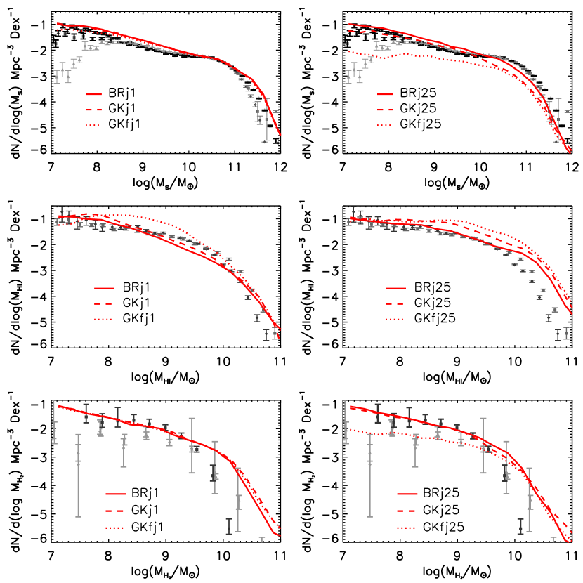
Figure 2: Top left - galaxy stellar mass functions (GSMFs) for all galaxies in the GKfj1 (dotted lines), GKj1 (dashed lines) and BRj1 (solid lines) models at $z=0$. The local GSMFs are overplotted, with Baldry et al. (2008, 2012) in bold above and Panter et al. (2007) and Li & White (2009) in bold below log M${}_{\ast}/\mbox{${\rm M}_{\odot}$}=10.65$ to emphasize where each is more reliable. Middle left - same as top left except for the ${\rm H}_{\rm I}$ mass functions at $z=0$, with the local HIMF from Zwaan et al. (2005a, gray) and Martin et al. (2010, black) overplotted. Bottom left - same as top left except for the H₂ mass functions (H2MFs) at $z=0$, with the local H2MFs for a constant and variable $X_{CO}$ factor from Keres et al. (2003, gray) and Obreschkow et al. (2009, black) overplotted. Right column - similar to left column except for the GKfj25 (dotted lines), GKj25 (dashed lines) and BRj25 (solid lines) models. The middle panels highlight how the ${\rm H}_{\rm I}$ gas content of galaxies can help to constrain galaxy formation models.

Figure 2 shows the $z=0$ GSMFs, HIMFs, and H2MFs for all of our models. We do not show the GKfjm, GKjm, and BRjm mass functions as they are the same as the GKfj1, GKj1, and BRj1 models respectively, since the gas is redistributed only in post-processing. As can be seen in the top row, the predicted $z=0$ stellar mass function is extremely similar for the $f_{j}=1$ models, and is in reasonable agreement with observations of the local GSMF. The $f_{j}=2.5$ models tend to produce too few galaxies with large stellar masses, with the largest discrepancy around the knee of the GSMF. Of the $f_{j}=2.5$ models, the BRj25 model is in the best agreement with the observed GSMF. In the models with extended gas distributions, the lower gas densities cause star formation to be less efficient. In the GK models, H₂ formation is more efficient in gas with higher metallicity, but more H₂ is photo-dissociated if the UV background is high. In the GK model with a fixed UV background, star formation becomes very inefficient in low mass, low-metallicity halos. In the GK model with a varying UV background, the UV radiation field intensity is also lower in these low-mass halos, which goes in the opposite direction, leading to a larger net fraction of H₂ and therefore less suppression of star formation relative to the GKf model.

We also find that the GK and BR extended disk ($f_{j}=2.5$) models produce reasonable agreement with the observed GSMF and galaxy star formation rate function for galaxies selected via their stellar emission at $z\sim 2$. We show these results along with a more detailed comparison of our model predictions with the optical properties of DLA host galaxies in Berry et al. (2014, in prep.).

The middle row of Figure 2 shows the HIMFs for the models along with local 21-cm observations from the HIPASS and ALFALFA surveys (Zwaan et al., 2005a; Martin et al., 2010), which highlights the power of using cold gas observations to discriminate between models. None of our models matches the observed ${\rm H}_{\rm I}$ mass function well in detail. The BRj1 and GKj1 models provide the best match to the observations, but produce slightly too few systems with intermediate ${\rm H}_{\rm I}$ masses ($10^{8}~{}\mbox{${\rm M}_{\odot}$}\lower 2.15277pt\hbox{$\;\buildrel<\over{\sim}\;$}M_{\rm HI}\lower 2.15277pt\hbox{$\;\buildrel<\over{\sim}\;$}10^{10}~{}\mbox{${\rm M}_{\odot}$}$). The GKfj1 model overproduces the number of systems with $M_{HI}\lower 2.15277pt\hbox{$\;\buildrel<\over{\sim}\;$}10^{9.5}~{}\mbox{${\rm M}_{\odot}$}$. The BRj25 and GKj25 models are more successful at reproducing the slope of the observed HIMF at low masses, but significantly overpredict the number of systems with high HI masses. The GKfj25 model produces too many galaxies at all HI masses. In general, the model HIMFs show that galaxies in the fixed-UV GK models have more HI than in the varying-UV and BR models, for the reasons discussed above. Similarly, galaxies with more extended gas distributions have more HI and shallower slopes for their HIMFs than the traditional disc models.

The bottom row of Figure 2 shows the $z\sim 0$ H2MFs for the models along with the inferred H2MF from the FCRAO Extragalactic CO survey (Keres et al., 2003) assuming a constant $X_{CO}=2\times 10^{20}$ factor and using a variable $X_{CO}$ factor as computed by Obreschkow et al. (2009). The H2MFs for the $f_{j}=1$ models are almost identical to each other and are in good agreement with both observational estimates at low M_H2, but overproduce the number of high-M_H2 systems. The predictions of the BRj25 and GKj25 models are very similar to the $f_{j}=1$ models, but have a slightly better fit at high-H₂ mass. the GKfj25 model produces substantially fewer systems with low M_H2, leading to a flatter H2MF low-mass end slope. For all four models, the high mass end of the H2MFs are in better agreement with the observational estimates of Keres et al. (2003), which assumed a constant conversion factor between CO and ${\rm H}_{2}$($X_{CO}$). However, the estimates obtained by Obreschkow et al. (2009) with a variable $X_{CO}$ are likely to be more accurate. In Keres et al. (2003), the highest mass bin contains a number of CO luminous starburst galaxies. PST14 provide a more detailed comparison between the observed CO luminosity function and the $f_{j}=1$ models.

In addition, PST14 show a comparison of the radial sizes of galaxies in the $f_{j}=1$ models with observations, finding good agreement for the HI radii and SFR half-light radii from $z=0$ to 2. The $f_{j}=2.5$ models produce SFR half-light radii that are still consistent with observations at $z=0$, but are about a factor of two larger than the $f_{j}=1$ model disks at $z=2$, in apparent conflict with observations. However, it is unknown to what extent the observed $z\sim 2$ star forming galaxies may be biased towards compact objects, due to selection. PST14 also show the ratio of HI mass to stellar mass, ratio of ${\rm H}_{2}$ mass to stellar mass, and ratio of HI to ${\rm H}_{2}$mass, as a function of galaxy stellar mass and surface density, showing good agreement with observations for $z=0$ disk-dominated galaxies in the $f_{j}=1$ models. We have carried out this comparison for the $f_{j}=2.5$ models as well, and find that relative to the $f_{j}=1$ models they tend to produce slightly higher gas fractions overall, and slightly less ${\rm H}_{2}$ relative to HI. However, the results are still within the uncertainty on the observational values.

3.2 Column Density Distribution

The ${\rm H}_{\rm I}$ column density distribution function, $f(\mbox{${N}_{\rm HI}$},X)$, is one of the best constrained observational quantities for ${\rm H}_{\rm I}$ absorption systems. It is defined as the number of absorbers with column densities in the range $[\mbox{${N}_{\rm HI}$},\mbox{${N}_{\rm HI}$}\ +d\mbox{${N}_{\rm HI}$}]$ per comoving absorption length $[X,X+dX]$

$$f_{HI}(\mbox{${N}_{\rm HI}$},X)d\mbox{${N}_{\rm HI}$}\ dX=n_{DLA}(\mbox{${N}_{\rm HI}$},X)$$ (7)

where $dX=\frac{H_{0}}{H(z)}(1+z)^{2}dz$. Absorption systems with a constant comoving density and proper size have a constant density per unit $X$ along the sight-line. Observations indicate only mild evolution in the column density distribution function with redshift (e.g. Prochaska & Wolfe, 2009).

The top panel of Figure 3 shows the predicted column density distribution function at $2<z<3.5$ for the $f_{j}=1$ models in the range $10^{19}<\mbox{${N}_{\rm HI}$}\ <10^{22.5}$ cm^-2 compared with the recent SDSS data release (DR9) results from Noterdaeme et al. (2012) and observations of sub-DLAs ($10^{19}<\mbox{${N}_{\rm HI}$}$) from Zafar et al. (2013). We can see that all models do moderately well at reproducing the number of high column density systems, but greatly underproduce the lower column density systems. This result has been shown before by Maller et al. (2001), and may indicate that the gas discs in the $f_{j}=1$ models are too compact. An alternative is that there are a large number of DLAs that are hosted in haloes below our resolution limit or that do not arise from gas in galactic discs, although neither of these effects seems to be very likely to make a large contribution, based on recent results from numerical simulations (e.g. Fumagalli et al., 2011; Cen, 2012). In addition, we find this scenario to be unlikely as they would have small velocity widths, inconsistent with observations.

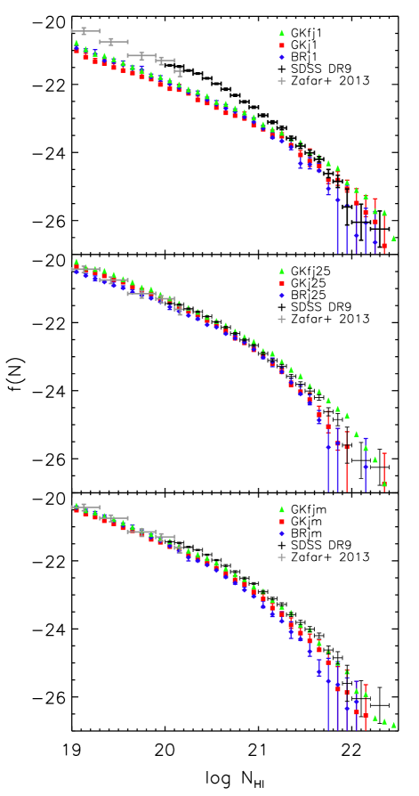
Figure 3: Top panel - column density distribution function for ${\rm H}_{\rm I}$ absorption systems in the $f_{j}=1$ models (GKfj1: green triangles; GKj1: red squares; BRj1: blue diamonds) in the redshift range $2<z<3.5$. Middle panel - same as top except for the $f_{j}=2.5$ models. Bottom panel - same as top except for the merger models (GKfjm: green triangles; GKjm: red squares; BRjm: blue diamonds). The model errors represent the maximum field-to-field variation for four subfields of $0.5\times 0.5$ deg^-2. The fixed- and varying-UV GK models have similar errors. The SDSS DR9 results from Noterdaeme et al. (2012) are overplotted in black and the sub-DLA results from Zafar et al. (2013) in gray. The $f_{j}=1$ models have a shallower slope in f(${N}_{\rm HI}$), causing them to produce too few low-${N}_{\rm HI}$ systems, which is most apparent at ${\rm log}~{}\mbox{${N}_{\rm HI}$}\ <21$. The $f_{j}=2.5$ models provide the closest fit and are a good match to the data.

Historically, no DLAs were known with column densities log N${}_{HI}>10^{22}$ cm^-2, and simulations had difficulty reproducing this very sharp cutoff (e.g. Nagamine et al., 2004a; Pontzen et al., 2008). Recently, larger volume surveys such as SDSS DR9 have revealed that although rare, these high HI column density systems do exist. We note that, in the paradigm in which metallicity is a fundamental parameter controlling the ${\rm H}_{\rm I}$-H₂ transition, it is more likely to produce high ${\rm H}_{\rm I}$ column density systems at high redshift as the threshold density for forming H₂ becomes higher for lower metallicity gas (e.g. Schaye, 2004; Erkal et al., 2012). In our models, this is reflected in the larger numbers of high column density systems predicted in the metallicity-dependent GK models. We include ${\rm H}_{\rm II}$ gas, but find it makes no significant difference to the predicted column density distribution.

Motivated by the discrepancies in the number of low column density systems in the models with $f_{j}=1$, we explore a simple model with a more extended distribution of cold gas with $f_{j}=2.5$. The middle panel in Figure 3 shows the column density distribution for the GKfj25, GKj25, and BRj25 models. These ‘extended gas’ models do significantly better than the $f_{j}=1$ models at matching the observed column density distribution function, reproducing the general shape of the column density distribution over a wide range of column densities. The BRj25 model is not as successful at reproducing the number of DLAs at all column densities especially at high-${N}_{\rm HI}$  specifically at log $\mbox{${N}_{\rm HI}$}\ \lower 2.15277pt\hbox{$\;\buildrel>\over{\sim}\;$}21.6$, although uncertainties due to cosmic variance are larger in this regime. Again, all models produce DLAs with log $\mbox{${N}_{\rm HI}$}\ \lower 2.15277pt\hbox{$\;\buildrel>\over{\sim}\;$}22$ cm^-2, although they are rarer in the BRj25 model than the GK models, due to the differing amount of gas and the density threshold for the ${\rm H}_{\rm I}$-${\rm H}_{2}$ transition, discussed further below. The success of the $f_{j}=2.5$ models suggests that either the gas that forms discs has higher specific angular momentum than the dark matter halo material, or DLAs arise from gas in an alternate extended distribution such as an outflow or tidal tails, although we have not specifically modeled these configurations here. The picture of DLAs arising from extended gas is supported by numerical simulations, which have shown that stellar driven winds can preferentially remove low-angular momentum material, leading to a higher average specific angular momentum (e.g. Brooks et al., 2011). In addition, the gas specific angular momentum can also be boosted by cold flows and mergers (Robertson et al., 2006a; Agertz et al., 2011; Stewart et al., 2013).

To explore the possible boosting of specific angular momentum by mergers, we also consider a simple merger-based model in which $f_{j}$ is increased following major and minor mergers, as described in Section 2.4. The resulting column density distribution for the GKfjm, GKjm, and BRjm models is shown in the bottom panel of Figure 3. Interestingly, these simple models do fairly well at reproducing the column density distribution over the whole range shown, much better than the $f_{j}=1$ models, although they slightly underproduce the number of DLAs at all ${N}_{\rm HI}$. As they contain the same amount of ${\rm H}_{\rm I}$ as the $f_{j}=1$ models, their success suggests that the cold gas may be in an extended distribution in a subset of galaxies due to the conditions of their formation.

At the low-${N}_{\rm HI}$ end of the column density distribution, sub-DLAs ($19<{\rm log}~{}\mbox{${N}_{\rm HI}$}\ <20.3$) in the $f_{j}=2.5$ models are in agreement with the results of Zafar et al. (2013), although our results become more uncertain at ${\rm log}~{}\mbox{${N}_{\rm HI}$}\ \lower 2.15277pt\hbox{$\;\buildrel<\over{\sim}\;$}19.5$. Low column density systems are more likely to have been produced in outflows and filaments of cold gas. Furthermore, the distribution of gas in exponential discs likely does not extend smoothly down to arbitrarily low-${N}_{\rm HI}$, and haloes below our mass resolution (log M${}_{h}/~{}\mbox{${\rm M}_{\odot}$}<9.5$) may also make a significant contribution to sub-DLAs. Therefore, we restrict the rest of our analysis to systems selected as DLAs ($\log~{}\mbox{${N}_{\rm HI}$}\ >20.3$ ${\rm atoms~{}cm}^{-2}$) as the majority are likely produced in cold dense gas that is closely associated with galaxies.

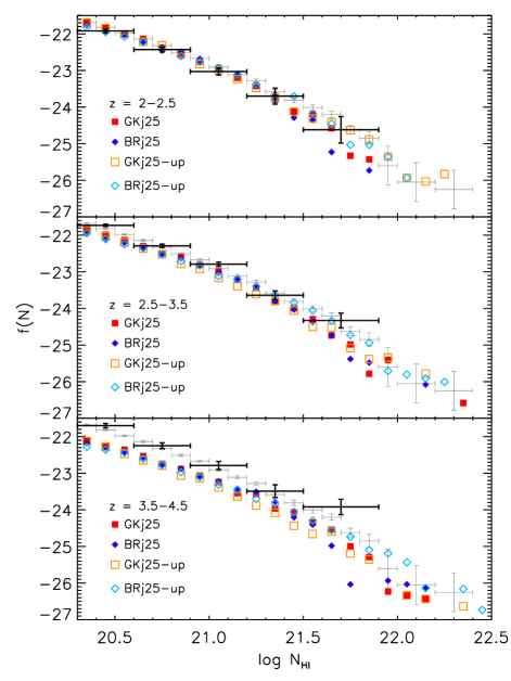
Figure 4: Similar to Figure 3 except the column density distribution function is plotted for DLAs at redshifts $2<z<2.5$ (top), $2.5<z<3.5$ (middle), and $3.5<z<4.5$ (bottom) in the GKj25 (red squares) and BRj25 (blue diamonds) models. Open points show the total cold neutral gas column density including H₂. Observations from SDSS DR5 (Prochaska & Wolfe, 2009) at the same redshifts are overplotted (black), along with the SDSS DR9 results at $2<z<3.5$ (gray) for reference. Both the models and observations show a flattening of the column density distribution at higher redshifts. Each model shows a decline in the number of low-${N}_{\rm HI}$ DLAs with redshift yet a comparable number of high-${N}_{\rm HI}$ DLAs. At $3.5<z<4.5$, observations produce this flattening with more high-${N}_{\rm HI}$ DLAs. Additionally, the unpartitioned models indicate that the HI-H₂ transition becomes important at log $\mbox{${N}_{\rm HI}$}\sim 21.7$, in qualitative agreement with the observations.

Figure 4 shows the column density distribution function at $2<z<2.5$, $2.5<z<3.5$, and $3.5<z<4.5$ for the GKj25 and BRj25 models with the SDSS DR5 observations at the same redshifts overplotted (Prochaska & Wolfe, 2009). The models at $2<z<3.5$ are consistent with observations, although at $3.5<z<4.5$, both produce fewer DLAs than are observed. The shape of the column density distribution functions become flatter at higher redshifts in both models, consistent with observations. However, in the models this flattening results in a reduced number of low-${N}_{\rm HI}$ systems in the highest redshift bin, which is in conflict with observations. All of our models fail to reproduce the observed number of DLAs at $z\lower 2.15277pt\hbox{$\;\buildrel>\over{\sim}\;$}3$ (see section 3.3), and we see this here reflected in the column density distribution.

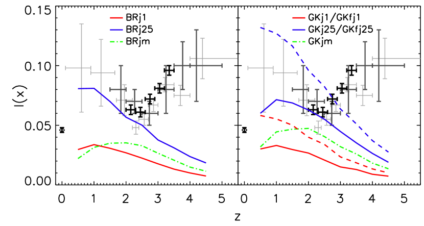
Figure 5: Left panel - the comoving line density of DLAs as a function of redshift for the BRj1 (red), BRj25 (blue), and BRjm (green dot-dashed) models. Right panel - same as the left except for the GKj1, GKjm, and GKj25 models with the GKfj1 and GKfj25 models (dashed) overplotted. Observations of Mg II absorbers (Rao et al., 2006) and high-redshift DLAs from Prochaska & Wolfe (2009) are overplotted in light gray while those from Zafar et al. (2013) are shown in dark gray. Observations of local galaxies (Zwaan et al., 2005b) and high-redshift DLAs (Noterdaeme et al., 2012) are overplotted in black. All models fail at $z>3$, and the $f_{j}=1$ models produce too few DLAs at all redshifts. The BRj25 and GKj25 models are in the best agreement with the observations at $z\lower 2.15277pt\hbox{$\;\buildrel<\over{\sim}\;$}2.5$, and the merger models are only a modest improvement over the $f_{j}=1$ models.

We also show the column density distribution function of the BRj25 and GKj25 models where gas is left unpartitioned, BRj25-up and GKj25-up respectively. In these models, the total cold neutral gas density, regardless of whether it is in HI or ${\rm H}_{2}$, is used to compute the column density, as in most previous models. These models allow us to study the effect of multiphase partitioning on the column density distribution function. We can see by comparing the partitioned and unpartitioned models that the ${\rm H}_{\rm I}$-${\rm H}_{2}$ transition does lead to a slightly steeper drop in the number of high column density systems. This transition can be seen in Figure 4 at log $\mbox{${N}_{\rm HI}$}\sim 21.7$, qualitatively consistent with observations. The small number of high-${N}_{\rm HI}$ systems causes there to be significant scatter at high column densities. Both models produce more DLAs with very high column densities at higher redshifts, while these very high-${N}_{\rm HI}$ DLAs are only seen in the unpartitioned models at $z\sim 2$, suggesting that the HI-H₂ transition may occur at lower density at high redshift.

3.3 Comoving line density and $\Omega_{\rm g}({\rm z})$

The column density distribution function gives the number of DLAs per unit absorption path length for a given column density. The zeroth moment of this distribution is the line density of DLAs, which measures the number of DLAs per comoving absorption distance:

$$l_{\rm DLA}(X)dX=\int^{\infty}_{N_{20.3}}~{}f_{\rm HI}(N,X)dN~{}dX$$ (8)

Figure 5 shows the comoving line density of DLAs as a function of redshift for the BR models (left) and fixed- and varying-UV GK models (right). Observational estimates of the line density of high redshift DLAs from Prochaska & Wolfe (2009) and Noterdaeme et al. (2012), and that inferred from Mg II absorbers from Rao et al. (2006) are also overplotted. As compared to the $f_{j}=1$ models, the larger ${\rm H}_{\rm I}$ masses in the BRj25 and GKj25 models, discussed in Section 3.1, are also reflected in the larger number of DLAs at all redshifts, in much better agreement with observations at $z\lower 2.15277pt\hbox{$\;\buildrel<\over{\sim}\;$}2.5$. The compact gas distributions of galaxies in the $f_{j}=1$ models cannot reproduce the observed number of DLAs at any redshift. Additionally, the merger-based models are only a modest improvement over the $f_{j}=1$ models. Relative to the other models, the GKfj25 model gives rise to significantly more DLAs at all redshifts. As we will see later, a large number of DLAs in the GKfj25 model are hosted in low mass dark matter haloes. These systems have low metallicity, and in the GKf models, they are inefficient at converting gas into ${\rm H}_{2}$ and subsequently into stars, so they have large ${\rm H}_{\rm I}$ masses. Therefore a large number are selected as DLAs, boosting the line density. The BRj25 and GKj25 models produce the best agreement with the data at $z<3$.

At $z>3$, all of our models produce far too few DLAs, and show the opposite trend as observations (the number density of DLAs decreases, rather than increases, with increasing redshift). The reasons for this fairly dramatic discrepancy are unclear. Two possible explanations are that an increasing number of DLAs are associated with gas in filaments or outflows at higher redshifts, or that the distribution of gas in galactic discs evolves over cosmic time. Note that the gas would have to be more extended at higher redshifts to alleviate this discrepancy.

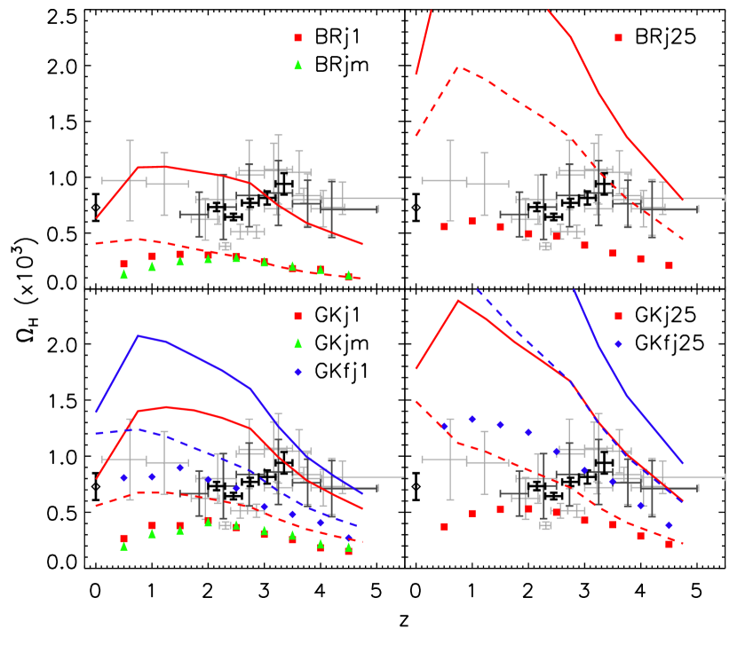
Figure 6: The cosmic density of ${\rm H}_{\rm I}$ contained in DLAs ($\Omega_{\rm DLA}$) as a function of redshift (solid shapes) and the amount of ${\rm H}_{\rm I}$ in all galaxies ($\Omega_{\rm HI}$; dashed line) along with the total amount of cold neutral gas in all galaxies $\Omega_{HI+H_{2}}$ (solid line). Observations of DLAs and Mg II absorbers (Zwaan et al., 2005a; Péroux et al., 2005; Rao et al., 2006; Prochaska & Wolfe, 2009; Noterdaeme et al., 2009; Guimarães et al., 2009) are overplotted in light gray. The dark gray observations of DLAs and sub-DLAs are from Zafar et al. (2013). Both the SDSS DR9 observations of high-redshift DLAs (Noterdaeme et al., 2012) and observations of local galaxies (Braun, 2012) are shown in black. Upper left panel - BRj1 (red squares) and BRjm (green triangles) models. Upper right panel - BRj25 model. Lower left panel - GKfj1 (blue diamonds), GKj1 (red squares), and GKjm (green triangles) models. Lower right panel - GKfj25 (blue diamonds) and GKj25 (red squares) models. The BRj25, GKj25, and GKfj1 models are in reasonable agreement with observations at $z\lower 2.15277pt\hbox{$\;\buildrel<\over{\sim}\;$}2.5$ while the GKj1, BRj1, and merger-based models underproduce $\Omega_{\rm DLA}$ at all redshifts. The GKfj25 model is the only model that is remotely close to the data at $z\lower 2.15277pt\hbox{$\;\buildrel>\over{\sim}\;$}2.5$, but it predicts $\Omega_{\rm DLA}$ somewhat higher than observational measurements at lower redshift, and the column density distribution is in conflict with observations.

Fumagalli et al. (2011) and Cen (2012) found that large amounts of DLA column density gas arise in filaments extending up to the virial radius at $z=4$. This fraction of DLA column density gas in filamentary structures is significant at $z\lower 2.15277pt\hbox{$\;\buildrel>\over{\sim}\;$}3$ and decreases monotonically with cosmic time, in keeping with the discrepancy between our models and observations. Moreover, the majority of missing DLAs in our models are at low-${N}_{\rm HI}$, as would be expected for intergalactic DLAs. If intergalactic DLAs, produced for example in filaments of cold gas, make up a significant fraction of the DLA population, then many DLAs will not be included in our models. Alternatively, if a significant number of high-redshift DLAs are associated with haloes of mass log (M${}_{h}/~{}\mbox{${\rm M}_{\odot}$})<10$, then the discrepancy might be a resolution effect since our simulations are incomplete below this mass. Since DLA metallicities at these redshifts are very low, and the formation of H₂ in this regime is not well-understood, the amount of neutral hydrogen gas in a given halo and the number of DLAs may be affected.

Using the column density distribution function and the comoving line density of DLAs, we can calculate the total neutral hydrogen gas mass density in DLAs using:

$$\Omega_{\rm DLA}=\frac{m_{H}H_{0}}{c\rho_{c,0}}\frac{\Sigma N(HI)}{\Delta X}$$ (9)

where $m_{H}$ is the mass of the hydrogen atom, $H_{0}$ is the Hubble constant, $\rho_{c,0}$ is the critical density at $z=0$, and the sum is calculated for systems with log N(HI)$>20.3$ across a total absorption pathlength of $\Delta X$. Figure 6 shows the total cold gas density ($\Omega_{\rm HI+H_{2}}(z)$), neutral hydrogen density in all galaxies ($\Omega_{\rm HI}(z)$), and the neutral hydrogen density inferred from systems selected as DLAs ($\Omega_{DLA}$) in the BRj1 and BRjm (top left) models; BRj25 (top right) model; GKfj1, GKj1, and GKjm (bottom left) models; and GKfj25 and GKj25 (bottom right) models. Observational estimates of $\Omega_{\rm DLA}(z)$ from DLAs and Mg II absorbers are overplotted for reference (Péroux et al., 2005; Rao et al., 2006; Noterdaeme et al., 2009; Prochaska & Wolfe, 2009; Guimarães et al., 2009; Braun, 2012; Noterdaeme et al., 2012). As can be seen in Figure 6, the $f_{j}=1$ and merger-based models underproduce the amount of $\Omega_{\rm DLA}(z)$. The GKfj1, GKj25 and BRj25 models produce the best fit to the $\Omega_{\rm DLA}(z)$ distribution. The GKfj1 model produces too few DLAs and too many high-${N}_{\rm HI}$ DLAs (see Figure 3), causing it to be a coincidence that it reproduces the observed amount of $\Omega_{DLA}$. On the other hand, the GKfj25 model produces too much ${\rm H}_{\rm I}$ while the BRj1, GKj1, and merger-based models produce too little ${\rm H}_{\rm I}$ at these redshifts. This is consistent with the conclusions drawn from their respective column density distribution functions and comoving line densities. As already anticipated from Figure 5, all of our models contain less ${\rm H}_{\rm I}$ in DLAs than is observed at $z\lower 2.15277pt\hbox{$\;\buildrel>\over{\sim}\;$}3$. Only the GKfj25 model is marginally consistent with the observations at these redshifts.

Note that the different models make different predictions for the total amount of cold gas in galaxies, as well as for the amount of ${\rm H}_{\rm I}$ in galaxies and the fraction of ${\rm H}_{\rm I}$ in systems that would have been selected as DLAs. The GKfj25 model predicts the largest amount of cold gas overall, as well as the highest values of $\Omega_{\rm HI}(z)$ and $\Omega_{\rm DLA}(z)$. This is because in this model, a lot of gas has low metallicity and is at low surface density, leading to inefficient ${\rm H}_{2}$ formation and star formation in many systems. It is interesting to note that while the total cold gas density and $\Omega_{\rm HI}$ tend to rise with decreasing redshift in all models, the fraction of gas in systems that are selected as DLAs decreases, leading to a flatter dependence of $\Omega_{\rm DLA}$ on redshift, in better agreement with observations. Overall, the $f_{j}=2.5$ models predict a lower fraction of HI to be contained in DLAs than the $f_{j}=1$ models. As high-${N}_{\rm HI}$ systems make the largest contribution to $\Omega_{\rm DLA}$ and the $f_{j}=1$ models have relatively more high-${N}_{\rm HI}$ DLAs due to a flatter column density distribution function, we expect a larger fraction of the total cold gas to come from the central regions of galaxies. Although there are more DLAs in the GKjm and BRjm models, the reduced number of high-${N}_{\rm HI}$ systems is evident as $\Omega_{\rm DLA}(z)$ for the GKjm model is comparable to the GKj1 and BRj1 models at all redshifts. An overproduction of high-${N}_{\rm HI}$ DLAs in the BRj1 model causes the inferred amount of HI in DLAs at $z\sim 4$ to be slightly larger than the total amount in all galaxies. In spite of a significant decrease in the number density of DLAs at $z>3$ in all models, the $\Omega_{\rm DLA}(z)$ distribution remains relatively flat. This result is in agreement with the flattening of the column density distribution as was discussed in section 3.2.

Returning to the discrepancy between our model predictions and observations at $z\lower 2.15277pt\hbox{$\;\buildrel>\over{\sim}\;$}3$, it is first interesting to note that in the BRj1 model, even the total cold gas density at $z\lower 2.15277pt\hbox{$\;\buildrel>\over{\sim}\;$}3$ is lower than the observational estimates of $\Omega_{\rm HI}$ from DLAs. Indeed, this model is quite similar to the model presented in S08, and this discrepancy has already been pointed out in that work (see their Figure 14). It can also be seen from the results presented in S08 that the predicted $\Omega_{\rm cold}$ at high redshift is quite sensitive to the assumed cosmological parameters, in particular the power spectrum normalization $\sigma_{8}$. This suggests that part of the problem may be due to too-efficient star formation and/or overly efficient ejection of gas by strong stellar winds at these epochs in these models.

At redshifts $z<2$, all of the models predict a relatively flat dependence of $\Omega_{\rm DLA}$ on redshift, in qualitative agreement with observations, although the normalization is too low in the BRj1/BRjm models and a bit high in the GKfj25 model. This is the case even in models (BRj25, GKj25) with much more rapidly rising total gas density and $\Omega_{\rm HI}$. The large amount of ${\rm H}_{\rm I}$ in galaxies that would not be selected as DLAs in the BRj25 and GKj25 models arises from ${\rm H}_{\rm I}$ in lower column density systems in low mass haloes (log M${}_{h}~{}/~{}\mbox{${\rm M}_{\odot}$}<10$), which have low gas surface densities and small DLA cross sections.

Taken together, our model results suggest that the rather flat dependence of $\Omega_{\rm DLA}$ on cosmic time from $4.5\lower 2.15277pt\hbox{$\;\buildrel<\over{\sim}\;$}z\lower 2.15277pt\hbox{$\;\buildrel<\over{\sim}\;$}1$ derived from observations of DLAs could be a cosmic coincidence: at $z\lower 2.15277pt\hbox{$\;\buildrel>\over{\sim}\;$}3$, $\Omega_{DLA}$ may be ‘contaminated’ by cold gas that is not closely associated with galaxies, while at lower redshifts ($z\lower 2.15277pt\hbox{$\;\buildrel<\over{\sim}\;$}3$), $\Omega_{DLA}$ may significantly underestimate the total atomic gas content of all galaxies. These results show the danger in assuming that $\Omega_{DLA}=\Omega_{\rm cold}$ or even $\Omega_{\mathrm{H}I}$.

3.4 DLA Halo Masses and Cross-sections

The DLA cross section represents the area in kpc² for which a galaxy’s gas surface density (corrected for inclination) would be high enough for it to be selected as a DLA. It is straightforward to compute this quantity in our models, as using our assumed density profile we can easily compute the projected area within which the column density is greater than ${\rm log}~{}\mbox{${N}_{\rm HI}$}\ >20.3$, which is its DLA cross section. Figure 7 shows the distribution of DLA cross sections as a function of halo mass for our sample of DLAs in the GKj1, GKj25, and BRj25 models at redshifts $z=1$, $z=2$, $z=3$, and $z=4$. We only show these models as each of the $f_{j}=1$ models has a similar distribution of DLA cross sections at a given halo mass as the GKj1 model. The GKj25 and GKfj25 models are also similar.

We can see that in all models and at all redshifts, DLAs are predicted to occupy haloes with a fairly broad range of masses, $10^{10}\mbox{${\rm M}_{\odot}$}\lower 2.15277pt\hbox{$\;\buildrel<\over{\sim}\;$}M_{h}\lower 2.15277pt\hbox{$\;\buildrel<\over{\sim}\;$}10^{12}\mbox{${\rm M}_{\odot}$}$. Moreover, the DLA cross-section versus halo mass relation evolves mildly with time in any of the models. This has implications for DLA kinematics which we explore in a later section.

The DLA cross-section at a given halo mass grows with cosmic time in all of our models. By $z=1$, DLAs in the $f_{j}=2.5$ models have halo masses and DLA cross sections that are both typically $\sim 1.5$ decades larger than at higher redshift while they both span a similar dynamic range. Conversely in the $f_{j}=1$ models, there is a significant fraction of small, compact DLAs at all redshifts and evolution is seen as an increase in the number of higher mass DLAs. Additionally, our merger tree mass resolution limit of $M_{\rm res}=10^{9.5}\,\mbox{${\rm M}_{\odot}$}$ and the completeness limit of the host halo catalog ($V_{\rm vir}=50$ km s^-1) also significantly reduces the number of low mass DLAs. These effects are relatively small at low redshift, especially in the $f_{j}=2.5$ models. However the average halo mass decreases with increasing redshift causing the mass resolution of our models to become increasingly important, especially in the $f_{j}=1$ models.

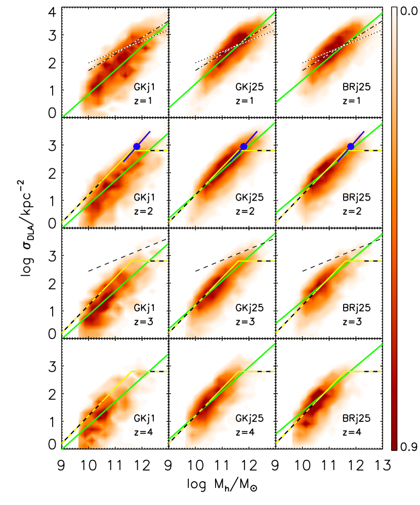
Figure 7: Number density distribution of DLA cross section versus halo mass for our sample of DLAs in the GKj1 (left column), GKj25 (middle column), and BRj25 (right column) models at $0.5<z<1.5$ (top row), $1.5<z<2.5$ (second row), $2.5<z<3.5$ (third row), $3.5<z<4.5$ (bottom row) with the best-fit slope of the $\mbox{${\sigma}_{\rm DLA}$}-M_{h}$ relation for each model at $z=2$ (green line). At high halo masses, the $\mbox{${\sigma}_{\rm DLA}$}-M_{h}$ relation flattens. The data point (blue circle and line) from Font-Ribera et al. (2012) shows their estimate for ${\sigma}_{\rm DLA}$ at $<z>~{}=2.3$ with the best-fit $\mbox{${\sigma}_{\rm DLA}$}-M_{h}$ slope. We also show the range of ${\sigma}_{\rm DLA}$ values and halo masses at $z\sim 3$ for several sets of numerical simulations: the best-fit power law at $1.4<z<4$ of Fumagalli et al. (2011, measured, yellow; extrapolated, yellow-black); and the best-fit power laws at $z=1$ (dotted), $z=1.6$ (dot-dashed), and $z=3$ (dashed) from Cen (2012). Compared to Font-Ribera et al. (2012), ${\sigma}_{\rm DLA}$, M_h, and $\alpha$ in the GKj25 model are in the best agreement. Conversely, the $f_{j}=1$ models produce ${\sigma}_{\rm DLA}$ and $\alpha$ values that are significantly lower than Font-Ribera et al. (2012).

Table 2: Halo mass vs. DLA cross-section ($M_{h}-\sigma_{DLA}$) Relation

	GKfj1	GKfj25	GKj1	GKj25	BRj1	BRj25	FR12
$<\mathrm{(log~{}M_{h}/M_{\odot})}>$	$4.9\times 10^{10}$	$5.3\times 10^{10}$	$8.3\times 10^{10}$	$1.1\times 10^{11}$	$8.5\times 10^{10}$	$8.6\times 10^{10}$	$6\times 10^{11}$
$<\mbox{${\sigma}_{\rm DLA}$}/\mathrm{kpc^{-2}}>^{\ast}$	490$\pm$450	1030$\pm$740	570$\pm$660	1120$\pm$850	570$\pm$660	900$\pm$710	1400
$\alpha$	0.86	0.86	0.90	0.91	0.78	0.88	1.1$\pm 0.1$

Our results for DLAs at $\langle z\rangle=2.3$ correspond to the same mean redshift as Font-Ribera et al. (2012). Note, $\alpha$ changes with halo mass where higher mass halos have flatter $M_{h}-\sigma_{DLA}$ relations.
^∗ for DLAs with $11.8<{\rm log~{}M_{h}}/\mbox{${\rm M}_{\odot}$}<12.2$ where the errors show the scatter about the mean.

Recently using observations of DLAs at $2<z<3.5$ from the BOSS survey, Font-Ribera et al. (2012, hereafter FR12) found that DLAs with a mean redshift of $<z>=2.3$, have a large range of halo masses with an average halo mass of M${}_{h}=6\times 10^{11}~{}\mbox{${\rm M}_{\odot}$}$. For DLAs residing in haloes of mass M${}_{h}\sim 10^{12}~{}\mbox{${\rm M}_{\odot}$}$, they also find a mean DLA cross-section of $\mbox{${\sigma}_{\rm DLA}$}\ =1400$ kpc², and a $\mbox{${\sigma}_{\rm DLA}$}-$M_h relation that scales as $\sigma_{DLA}\propto$ M${}_{h}^{\alpha}$ where $\alpha=1.1\pm 0.1$ with a minimum halo mass of M${}_{h}=10^{9}~{}\mbox{${\rm M}_{\odot}$}$. In order to make an accurate comparison to Font-Ribera et al. (2012), we select all DLAs in each of our models with redshifts $2<z<2.6$, which corresponds to a mean redshift of $\langle z\rangle=2.3$. Table 2 shows our M_h, ${\sigma}_{\rm DLA}$, and $\alpha$ values for DLAs in each of our models. Our $f_{j}=2.5$ models produce DLAs with halo masses and DLA cross sections that are the most similar to Font-Ribera et al. (2012). The BRj25 and GKj25 models produce slopes of $\alpha\sim 0.9$, significantly flatter than that calculated in FR12. The second row of Figure 7 shows model DLAs that are at a comparable redshift to these observations. This also shows that the $f_{j}=2.5$ models produce the most comparable DLA cross sections in massive haloes $M_{h}\simeq 10^{12}\,\mbox{${\rm M}_{\odot}$}$ as FR12. The $f_{j}=1$ models produce significantly lower values of ${\sigma}_{\rm DLA}$.

Font-Ribera et al. (2012) also find that DLA halo mass does not correlate with column density. This result indicates that the column density distribution function has a similar shape at low and high halo mass. When we divide our sample in half based on halo mass (${\rm log}~{}M_{h}/\mbox{${\rm M}_{\odot}$}>10^{11}$, ${\rm log}~{}M_{h}/\mbox{${\rm M}_{\odot}$}<10^{11}$), we also find no correlation between DLA halo mass and column density. The results of Font-Ribera et al. (2012) strongly support the picture of a significant population of DLAs at $z\sim 2.3$ arising from extended gas associated with more massive galaxies.

We also compare our results to predictions from several different numerical hydrodynamic simulations. We overplot the results from Fumagalli et al. (2011) at $z=1.4-4$, and at $z=1.0,~{}1.6,~{}3.1$ from Cen (2012) in Figure 7. DLAs in the GKj1 model are more compact than DLAs observed in any numerical simulation at any redshift. In contrast, the BRj25 and GKj25 models are in very good agreement with the results of Fumagalli et al. (2011). Our $f_{j}=2.5$ models are in fair agreement with the predictions of Cen (2012) at $z=1$ while DLAs in our models have a much steeper $\mbox{${\sigma}_{\rm DLA}$}-$M_h relation. At $z\sim 3$, Cen (2012) finds much larger ${\sigma}_{\rm DLA}$ values at a given halo mass than our models or the other simulations predict. This appears to be due to outflows boosting the DLA cross-section. Our models do not directly model outflows, although they may indirectly contribute to our extended disk models. Note that an increasing contribution to the DLA cross-section from outflows or filaments with increasing redshift could manifest in just this way, as larger values of $\sigma_{\rm DLA}$ at a given halo mass.

At $z\sim 4$, more DLAs may arise in haloes below our resolution limit since our models show a decrease in halo mass and ${\sigma}_{\rm DLA}$ with redshift, especially in the GKj1 model. However, the gas fraction in haloes with $\log M_{h}/\mbox{${\rm M}_{\odot}$}\lower 2.15277pt\hbox{$\;\buildrel<\over{\sim}\;$}9.5$ also drops rapidly due to the “squelching” of gas infall by the photoionizing background after re-ionization implemented in our models. At $z<3$, the steep slope and low fraction of low-halo mass DLAs (M${}_{h}\sim 10^{10}~{}\mbox{${\rm M}_{\odot}$}$) in the $f_{j}=2.5$ models suggests that there are likely not many DLAs arising in haloes below our resolution limit. If ${\sigma}_{\rm DLA}$ at a given halo mass also increased with redshift, then we would expect even more DLAs to arise in these low mass haloes. Both Fumagalli et al. (2011) and Cen (2012) discuss the contribution of DLAs arising from streams and clumps to the DLA population at higher redshifts, although the simulations from Cen (2012) only probe haloes more massive than M${}_{h}>10^{10.5}~{}\mbox{${\rm M}_{\odot}$}$. At $z\sim 3-4$, both find that a large fraction of DLAs originate in filamentary structures and gas clumps extending as far as the virial radius. Conversely at $z<3$, these intergalactic DLAs make a much smaller contribution to the total DLA population, in keeping with the picture suggested by our results.

3.5 Metallicities

Figure 8 shows the distribution of cold gas-phase metallicities for all galaxies identified as DLAs at $2<z<3.5$ in all of our models compared with SDSS-DR3 and SDSS-DR5 results from observed DLAs in the same redshift range from Rafelski et al. (2012). In this initial set of plots, we show the mass-weighted mean metallicity of the cold gas in our model galaxies. Later, we consider the effects of metallicity gradients.

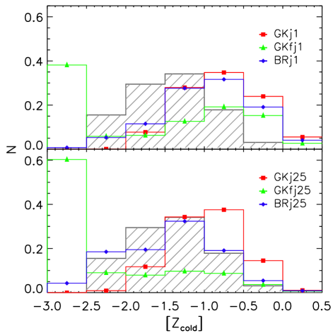
Figure 8: Upper panel - distribution of metallicities for all DLAs in the redshift range $2<z<3.5$ for the GKfj1 (red), GKj1 (green), and BRj1 (blue) models in the upper panel. Lower panel - same as top except for the GKfj25 (red), GKj25 (green), and BRj25 (blue) models. The observed distribution of DLA metallicities in the same redshift range are overplotted in gray (Rafelski et al., 2012). All the models except GKfj25 produce a distribution with a width similar to that of the observed one, with the BRj25 model producing the best agreement with the observed DLA metallicity distribution. The GKfj1 and GKfj25 models produce a significant number of DLAs with metallicities near the “pre-enriched” metallicity (${\rm log}~{}Z=-3$).

Our $f_{j}=1$ and GKj25 models show a roughly lognormal distribution of DLA metallicities with a peak around log Z $\sim$ -0.8. Both the fixed-UV models show flatter distributions with a large fraction of DLAs with metallicities near the pre-enriched metallicity of log Z $\sim-3$, indicating that a substantial number have never undergone significant star formation. We discuss these interesting systems further in a moment. DLAs in the merger-based models exhibit metallicity distributions very similar to the $f_{j}=1$ models, and so are not shown. Both the GKj25 and the BRj25 models are a good fit to the observed metallicity distribution in both the average metallicity and width. We note that at $z>3$, our models begin to miss a substantial fraction of DLAs, which likely have lower metallicities on average. This would have the effect of skewing the observed distribution to lower metallicities.

The population of very low metallicity, ${\rm H}_{\rm I}$-rich, nearly “pristine” galaxies predicted by the metallicity-based, fixed-UV GK models is interesting. Scaling the UV radiation field by the galaxy’s star formation rate increases the H₂ fraction in low mass galaxies relative to the model with a UV field fixed to the MW value, allowing these galaxies to form significant stellar components. In the fixed-UV models, the “pristine” galaxies are hosted by low-mass haloes (log (M${}_{h}/\mbox{${\rm M}_{\odot}$})\lower 2.15277pt\hbox{$\;\buildrel<\over{\sim}\;$}10$) and have stellar masses below log M${}_{\ast}/\mbox{${\rm M}_{\odot}$}<6.5$. A feature of the metallicity-based picture for ${\rm H}_{2}$ formation is that if gas is low metallicity and low density, ${\rm H}_{2}$ formation is extremely inefficient, the galaxy forms few stars and the gas never becomes enriched, so star formation stalls out. Star formation can be “kick-started” — if the galaxy manages to form even a small amount of stars, e.g. through a merger-triggered burst, this enriches the gas leading to more star formation and enrichment, and the galaxies rather quickly become enriched to significant levels — hence the double peaked distribution. The population of “pristine” haloes is more prevalent in the GKfj25 model because the extended gas configuration leads to more low surface density gas. A similar population has recently been reported in numerical hydrodynamic simulations using a similar metallicity-based prescription for ${\rm H}_{2}$ formation (Kuhlen et al., 2013). It is interesting that DLAs are observed down to log Z = -2.5, but no DLAs have been conclusively shown to have metallicities as low as the “pristine” haloes in the fixed-UV GK models, although they could have been detected if they existed. The presence of a DLA metallicity floor of log Z $\;\buildrel>\over{\sim}\;$ -2.6 has been discussed by Wolfe et al. (2005) and Rafelski et al. (2012) while systems with lower metallicities have been observed in the Ly$\alpha$ forest (Schaye et al., 2003; Simcoe et al., 2004). Qian & Wasserburg (2003) model star formation in DLAs with a chemical evolution code and find that star formation in pristine gas enriches it quickly, making the probability of detecting a DLA with log Z $\;\buildrel<\over{\sim}\;$ -2.6 very small. Additionally, we consider whether these pockets of “pristine” gas could really be common at intermediate redshifts, or whether this prediction perhaps reflects limitations in our understanding of how ${\rm H}_{2}$ formation and star formation take place in these environments. We also note that Gnedin & Kravtsov (2010) report that their fitting formulae, used in our GK models, may become unreliable below ${\rm log}~{}Z\lower 2.15277pt\hbox{$\;\buildrel<\over{\sim}\;$}-2.5$.

Figure 9 shows the probability of selecting a DLA with a given metallicity as a function of redshift for DLAs in the GKfj25 (top), GKj25 (middle), and BRj25 (top) models compared with observational estimates from Rafelski et al. (2012). We also show the best linear fits to DLA metallicity as a function of redshift for each model ([Z] $=\alpha z-[Z0]$). In order to examine the trends with redshift, we exclude DLAs with metallicities below log Z $<-2.5$ from the fits. Although all of our models predict a shallower evolution in $Z$ with redshift than seen in by Rafelski et al. (2012), the agreement with observations is considerably better than in many previous studies. Moreover, our results are also in agreement with Jorgenson et al. (2013) who found evidence for a lack of metallicity evolution over the redshift range $2.2<z<4.4$. We present our best-fit parameters and those from Rafelski et al. (2012) and Jorgenson et al. (2013) in Table 3. We can see that the population of “pristine” DLAs predicted by the GKfj25 model is present at all redshifts, and the distribution of metallicities in the ‘enriched’ population is as broad as that in the BR models. From this plot, it is apparent that the metallicities of DLAs in our models are in better agreement with the observational estimates in the lower part of the redshift range, $z\lower 2.15277pt\hbox{$\;\buildrel<\over{\sim}\;$}2$.

Table 3: DLA Metallicity vs. redshift Best-Fit Parameters

	$\alpha_{\small\frac{dZ}{dr}=0}$	$[Z0]_{\small\frac{dZ}{dr}=0}$	$\alpha_{\small\frac{dZ}{dr}=-0.1}$	$[Z0]_{\small\frac{dZ}{dr}=-0.1}$
GKfj1	-0.10	-0.61	-0.07	-0.93
GKfj25	-0.11	-1.03	-0.01	-1.55
GKj1	-0.11	-0.64	-0.09	-0.91
GKj25	-0.15	-0.55	-0.19	-0.60
BRj1	-0.14	-0.43	-0.12	-0.71
BRj25	-0.09	-1.10	-0.08	-1.32
R12∗	-0.22	-0.65	-	-
J13∗	-0.04	-1.06	-	-

Linear fits ([Z] = $\alpha z+{\rm[Z0]}$) for DLAs at $z<5$
^∗ observations of DLAs at $z<5$ from Rafelski et al. (2012) and $2.2<z<4.4$ from Jorgenson et al. (2013)

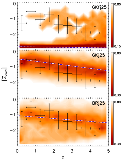
Figure 9: Conditional probability of DLA metallicity as a function of redshift in the GKfj25 (top), GKj25 (middle), and BRj25 models (bottom). The best linear fits to the average metallicities for DLAs with ${\rm log}~{}{\rm Z}>-2.5$ (to exclude the very low metallicity population) are overplotted (blue and white). Observation of DLAs from Rafelski et al. (2012) with the $1\sigma$ scatter in DLA metallicity are also overplotted. The GKj25 and BRj25 models show a shallow decrease in metallicity with increasing redshift, similar to observations, although the normalization is higher by $\sim 0.5$ dex in the GKj25 model. A significant number of DLAs in the GKfj25 model have metallicities near the “pre-enriched” metallicity, indicating that essentially no star formation has occured in these objects.

Results from integral field unit spectroscopy (e.g. Förster Schreiber et al., 2006) indicate that star-forming galaxies at $z\sim 2$ exhibit typical metallicity gradients of $dZ/dr=$ 0 to -0.3 dex kpc^-1 (Jones et al., 2010; Pilkington et al., 2012; Swinbank et al., 2012) and up to $dZ/dr\sim-0.4$ dex kpc^-1 in quasars (Jones et al., 2013). If DLAs sample the outskirts of galaxies, e.g. with impact parameters of b $\sim 10$ kpc at $2<z<3.5$ (typical in our extended disc models), a metallicity gradient could have a significant effect on typical DLA metallicities. Moreover, metallicity gradients in star-forming galaxies are typically measured along the disc while DLA column density gas likely also samples a significant amount of cold gas above the disc where metallicities are almost certainly lower. Recently, Fu et al. (2013) studied the effects of metallicity gradients in semi-analytic models and found they depend on the fraction of metals directly injected into the halo as well as recent mergers, which can re-establish a metallicity gradient. Following the observational studies mentioned above, we implement a metallicity gradient of ${\rm dZ/dr}=-0.1$ dex kpc^-1 where the average galaxy metallicity is set to the radius of the average cold gas mass ($r_{ave}=1.678r_{g}$). Thus, galaxies with larger cold gas masses will have more extended cold gas distributions. In general, DLAs arising in these galaxies will have larger impact parameters and subsequently be more affected by a metallicity gradient. As H₂ formation in the GK models is metallicity-dependent, if included self consistently, metallicities gradients could also affect other galaxy properties, and might produce results that are different in detail from those shown here. We show the results of the post-processed gradients only to qualitatively illustrate how they can potentially affect the distribution of DLA metallicities. However in the BR models, H₂ forms based on the midplane pressure, so introducing metallicity gradients would not impact other galaxy properties.

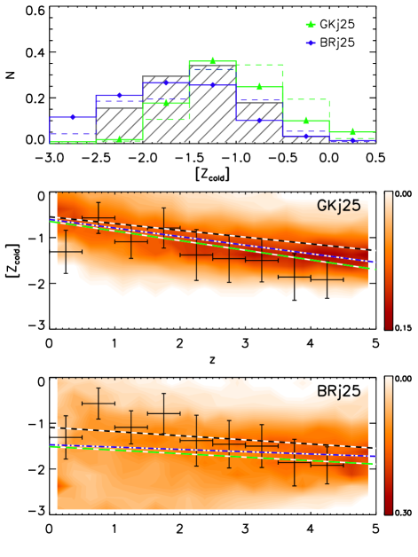
Figure 10: Top panel - predicted distribution of metallicities for DLAs at $2<z<3.5$ with a metallicity gradient ($dZ/dr=-0.1$ dex kpc^-1, solid) and without one (dashed). We exclude the fixed-UV and $f_{j}=1$ models for clarity as they exhibit similar shifts in metallicity. Observations of DLAs from Rafelski et al. (2012) are also shown in gray. Middle and bottom panels - conditional probability of DLA metallicity versus redshift including a metallicity gradient as above, for the GKj25 and BRj25 models respectively. Best linear fits (${\rm log}~{}Z>-2.5$) for three metallicity gradients are overplotted: $dZ/dr=0$ dex kpc^-1 (black and white dashed line), $dZ/dr=-0.1$ dex kpc^-1 (blue and white dot-dashed line), and $dZ/dr=-0.2$ dex kpc^-1 (green and white long-dashed line). Metallicity gradients can have a significant impact on the DLA metallicity and its evolution.

The top panel of Figure 10 shows the distribution of DLA metallicities in the redshift range $2<z<3.5$ before and after implementing a metallicity gradient. For $dZ/dr=-0.1$ dex kpc^-1, the average shift in DLA metallicity is $\Delta Z=[Z_{\rm DLA}]-[Z_{\rm gal}]\sim-0.3\pm 0.4$ with a tail extending to $\Delta Z<-1$. DLAs in each of our models have a similar average shift in metallicity. The broadened distribution reflects the large scatter in impact parameter, which can be as high as tens of kpc, explaining the tail to low metallicities. Although it is possible for the outskirts of galaxies to have metallicities below log Z$=-3$, we set this as the floor to the DLA metallicity as it corresponds to the metallicity of pre-enriched gas. The predicted mean metallicity of DLAs in this redshift range in our models is now in quite good agreement with the observations, and the shape of the distribution in the BRj25 models is in good agreement with the observations, though it does produce more systems with very low metallicities. The addition of a metallicity gradient causes the GKj25 model to move into better agreement with observations.

The middle and bottom panels of Figure 10 show the conditional probability distribution of DLA metallicities with a metallicity gradient $dZ/dr=-0.1$ dex kpc^-1 as a function of redshift for the GKj25 and BRj25 models. The linear fits to models with imposed metallicity gradients of $dZ/dr=0$ dex kpc^-1, $dZ/drZ=-0.1$ dex kpc^-1, and $dZ/dr~{}=-0.2$ dex kpc^-1 are shown for reference. Metallicity gradients cause a systematic shift in the redshift-metallicity relation for the BRj25 model while they make the slope steeper in the GKj25 model.

These trends indicate that sightlines through DLAs in the BRj25 model are sampling similar impact parameters relative to the distribution of cold gas at all redshifts, while those in the GKj25 model are preferentially selecting larger impact parameters at higher redshift. On the other hand, Fumagalli et al. (2011) and Cen (2012) found cold gas to be more extended at higher redshifts, coming from nearby streams flowing into the galaxy.

Overall, the addition of a metallicity gradient yields DLA metallicities in the GKj25 model in better agreement with observations, where stronger metallicity gradients make the above effects more pronounced. We find that a metallicity gradient of $dZ/dr\sim-0.3$ dex kpc^-1 would be needed to bring the GKj25 metallicities into agreement with observations while no fixed metallicity gradient produces satisfactory results with the BRj25 model. In reality, the slope of the metallicity gradient probably varies from galaxy to galaxy and may be correlated with other galaxy properties. However, this simple exercise highlights the importance of understanding and accounting for metallicity gradients in modeling absorption systems.

Pontzen et al. (2008) found DLA metallicity to be correlated with halo mass, where the majority of low metallicity DLAs (log $Z\lower 2.15277pt\hbox{$\;\buildrel<\over{\sim}\;$}-1.5$) were found in haloes with masses $M_{h}<10^{9.5}$ M_⊙. By comparison, our simulations do not probe this mass range and we find the typical DLA to reside in much higher mass haloes. We also look for a similar trend between halo mass and metallicity by dividing our sample roughly in half based on halo mass (M${}_{h}<10^{11}~{}\mbox{${\rm M}_{\odot}$}$, M${}_{h}>10^{11}~{}\mbox{${\rm M}_{\odot}$}$), and comparing their metallicity distributions. For each model, DLAs with halo masses $M_{h}<10^{11}$ ${\rm M}_{\odot}$make up the vast majority of low metallicity systems where the difference in metallicity for each subset ranges from -0.5 to -1.0 dex. Finally, Neeleman et al. (2013) find a correlation between ${N}_{\rm HI}$ and metallicity where DLAs with higher column densities have higher metallicities. We also see a similar, but weak trend in our model DLAs. Interestingly, the addition of a metallicity gradient causes this correlation to be stronger as it causes sightlines that sample the interior regions of galaxies to preferentially have higher metallicities than those sampling the outskirts of galaxies. Therefore, a strong correlation between metallicity and ${N}_{\rm HI}$ may also be suggestive of the presence of metallicity gradients in DLAs. A more detailed comparison between metallicities measured through absorption studies and via emission lines in star-forming galaxies, will be presented in Berry et al. (2014, in prep.).

3.6 Kinematics

Observationally, low ionization line profiles in DLAs exhibit multiple components with small individual velocity dispersions, yet the relative velocities between each component can be quite large. Therefore, Prochaska & Wolfe (1997) defined a number of statistical measures to probe the characteristics of line profiles. The velocity interval, $\Delta v_{90}$, is defined as the difference in velocity between the pixel containing 5% and 95% of the total optical depth. We calculate this statistic for each of our DLAs based on their low ionization absorption line profiles as detailed in Section 2.5. This quantity has proven to be the most difficult to reproduce in theoretical models, so we focus on $\Delta v_{90}$ for our analysis.

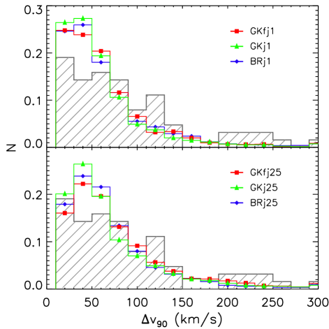
Figure 11: Upper panel – distribution of $\Delta v_{90}$ values for DLAs in the redshift range $2<z<3.5$ for the GKfj1 (red), GKj1 (green), and BRj1 (blue) models. Lower panel – same as top except for the GKfj25 (red), GKj25 (green), and BRj25 (blue) models. The observed $\Delta v_{90}$ distribution from Neeleman et al. (2013) is overplotted for reference. The GKj25 model has a $\Delta v_{90}$ distribution most consistent to observations of high-redshift DLAs. DLAs with $\Delta v_{90}>300$ km s^-1 are shown at $\Delta v_{90}=300$ km s^-1. The $f_{j}=1$ models produce too many low-$\Delta v_{90}$ DLAs as has been shown in previous analyses of DLAs in semi-analytic models (e.g. Maller et al., 2001).

Figure 11 shows the distribution of velocity widths, $\Delta v_{90}$, for DLAs in the $f_{j}=1$ and $f_{j}=2.5$ models with the $\Delta v_{90}$ values measured from observed DLAs overplotted (Neeleman et al., 2013). Historically, hierarchical models have had difficulty reproducing this distribution, tending to overproduce low-$\Delta v_{90}$ objects and underproduce the number of high-$\Delta v_{90}$ systems (e.g. Maller et al., 2001; Pontzen et al., 2008). The $f_{j}=1$ models have $\Delta v_{90}$ distributions that peak at low $\Delta v_{90}$, which is due to the large number of DLAs hosted by low-mass dark matter haloes. On the other hand, the $f_{j}=2.5$ models are noticeably better at reproducing the observed distribution of $\Delta v_{90}$. Table 4 shows the probability that the distribution of DLA $\Delta v_{90}$ values in each model are taken from the same distribution as the observed $\Delta v_{90}$ values as well as the D-statistic from the Kolmogoroz-Smirnov test. All $f_{j}=1$ models have a $\lower 2.15277pt\hbox{$\;\buildrel<\over{\sim}\;$}1\%$ chance of being from the same distribution as the observed $\Delta v_{90}$ values. However, the $f_{j}=2.5$ models are more successful, with the GKj25 model producing the most realistic $\Delta v_{90}$ distribution with a probability of 27%. This kinematic distribution is a significant improvement over those from previous semi-analytic models (e.g. Maller et al., 2001, 2003) and many numerical simulations. Our models do not include other effects such as galactic winds or cold accretion, which will likely increase the $\Delta v_{90}$ value of a given DLA (e.g. Cen, 2012). Note that the $f_{j}=1$ models are in slightly better agreement with the data than the $f_{j}=1$ discs from previous semi-analytic models (e.g. see Figure 1 in Maller et al., 2001).

Table 4: DLA $\Delta v_{90}$ K-S Test

	D	PK-S
GKfj1	0.18	2.5e-4
GKfj25	0.14	0.017
GKj1	0.23	2.5e-3
GKj25	0.12	0.27
BRj1	0.23	2.6e-3
BRj25	0.18	0.035

For DLAs at $2<z<3.5$, compared to observations from Neeleman et al. (2013).

The improvement in the $\Delta v_{90}$ distribution in the $f_{j}=2.5$ models is primarily due to two effects. Most importantly, more extended cold gas discs cause DLAs to originate in more massive haloes with larger rotational velocities, as we saw in Figure 7. As a secondary effect, more extended gas distributions make it more likely for DLAs to arise from ‘multiple hits’ or lines of sight passing through more than one galaxy within a parent halo. The large number of low mass galaxies in the GKfj25 model causes an excess of DLAs with low $\Delta v_{90}$ values. The improved success of the $f_{j}=1$ models is due to the increased cold gas masses of DLAs in all models causing more higher mass DLAs to be selected. We note that when cold gas discs are made very thin (e.g. very small values of $\chi_{z}$), the $\Delta v_{90}$ distributions also become peaked at low values.

The upper row of Figure 12 shows the distribution of halo masses for DLAs in our models over the redshift interval $2<z<3.5$. The lower row shows the probability of finding a DLA with a given $\Delta v_{90}$ value at a given halo mass at the same redshift. The average disc circular velocity and $1\sigma$ scatter for galaxies at a given halo mass are also overplotted. We find a similar trend between $\Delta v_{90}$ and disc velocity as Haehnelt et al. (1998) who found that $\Delta v_{90}$ tracked disc velocity following $\Delta v_{90}\sim 0.6v_{\rm disc}$ with a large scatter. As can be seen in the top and bottom panels of Figure 12, the extended gas distributions cause DLAs in the $f_{j}=2.5$ models relative to the $f_{j}=1$ models, specifically the GKj25 and BRj25 models, to originate from more massive haloes, which in turn have higher disc velocities. Conversely, the large number of pristine systems in very low mass haloes in the fixed-UV GK models lowers the average halo mass and $\Delta v_{90}$ value relative to the other models. DLAs with large $\Delta v_{90}$ values and low halo masses typically arise from ‘multiple hits’, which are more common in the $f_{j}=2.5$ models as can be seen in the bottom row of Figure 12.

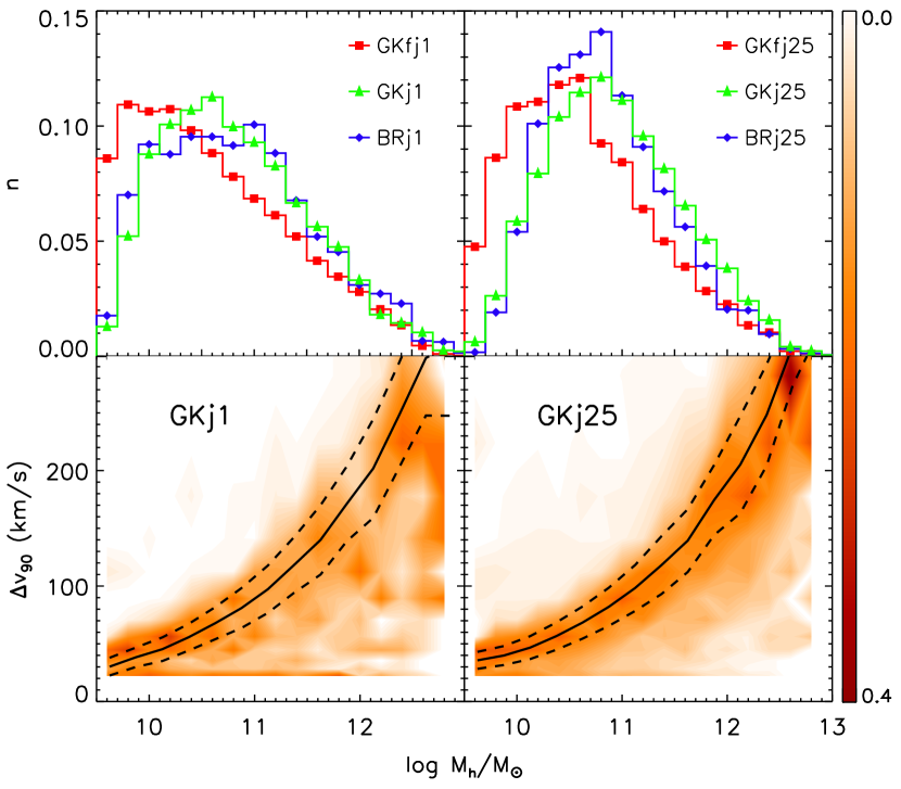
Figure 12: Upper left - histogram of the fraction of DLAs with a given halo mass for the GKfj1 (red), GKj1 (green), and BRj1 (blue) models at $2<z<3.5$. Upper right - same as upper left except for the GKfj25 (red), GKj25 (green), and BRj25 (blue) models. Lower left - conditional probability of $\Delta v_{90}$ versus DLA halo mass for the GKj1 model. Lower right - same as lower left except for the GKj25 model. The BRj1 and BRj25 models produce similar $\Delta v_{90}$-halo mass relations as the GKj1 and GKj25 models respectively. The average disc velocity (solid line) and $1\sigma$ scatter (dashed lines) are overplotted for reference. The higher halo masses of DLAs in the $f_{j}=2.5$ models cause them to produce more high-$\Delta v_{90}$ systems. DLAs with low halo mass and high $\Delta v_{90}$ values seen in the bottom row arise from ‘multiple hits’ or lines of sight passing through more than one galaxy in the same halo.

Figure 13 shows the conditional probability distribution of DLA metallicity as a function of $\Delta v_{90}$ for the GKfj25, GKj25, and BRj25 models. The best-fit power law to the metallicity-$\Delta v_{90}$ relation for our models and observations is also shown for reference, and the best-fit parameters are given in Table 5. In the $f_{j}=2.5$ models, systems with high $\Delta v_{90}$ values have metallicities comparable to observations, while they are slightly higher in the $f_{j}=1$ models. At low $\Delta v_{90}$, DLAs in the BRj25 model are in reasonable agreement with observations while those in the GKj25 model typically have slightly larger metallicities than is observed. Alternatively, the GKfj25 model produces a significant number of low metallicity, low $\Delta v_{90}$ systems, but again the metallicity distribution of these objects is peaked towards lower values in the models than the observations indicate. DLAs in the $f_{j}=1$ models are not shown as they predict metallicities and $\Delta v_{90}$ values that are significantly higher and lower, respectively, than observations.

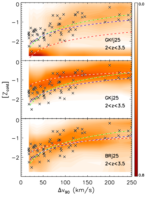
Figure 13: Conditional probability of $\Delta v_{90}$ versus metallicity for DLAs in the redshift range $2<z<3.5$. Top panel - GKfj25 model. Middle panel - GKj25 model. Bottom panel - BRj25 model. The best-fit power law for each model is shown by the red and white dashed line. We overplot the observed DLA $\Delta v_{90}$ versus metallicity relation from Wolfe et al. (2005, crosses), Ledoux et al. (2006, green dot-dashed line), and Jorgenson et al. (2013, blue dashed line). All models show evidence for an increase in metallicity with $\Delta v_{90}$, where the BRj25 model is in the best agreement with observations while the GKj25 model does not produce any very low-Z DLAs. At high $\Delta v_{90}$, the BRj25 model produces DLAs with metallicities in good agreement with observations.

Numerous authors have proposed that the $\Delta v_{90}$-metallicity relation may be the DLA version of the well-known mass-metallicity relation (e.g. Prochaska et al., 2008; Møller et al., 2013; Neeleman et al., 2013, and references therein). If the motions of neutral clouds giving rise to the $\Delta v_{90}$ values are governed by gravity whether it is rotation, infall, or outflow, then $\Delta v_{90}$ could be correlated with mass. Indeed, as shown in Figure 12, our models do predict a relationship between $\Delta v_{90}$ and halo mass, although with significant scatter. Similarly, we find galaxies with large $\Delta v_{90}$ values to be more likely to have higher metallicities. At all values of $\Delta v_{90}$, there is significant scatter in DLA metallicity, which is likely affected by galaxy inclination, the stochasticity of neutral clump properties, and infalling or outflowing gas. Moreover, we do find that the presence of a metallicity gradient in all DLAs has the effect of increasing the scatter of the $[Z]-\Delta v_{90}$ distribution as the high-$\Delta v_{90}$ DLAs are selected from higher mass haloes with a larger range of impact parameters. For this reason, we note that a metallicity gradient can weaken the connection between metallicity and $\Delta v_{90}$. Observations of star-forming galaxies show a large range in metallicity gradients, suggesting that this may also be the case in DLAs. Overall, metallicity gradients may contribute to the low observed metallicities and large scatter seen in DLAs.

Table 5: DLA Metallicity vs. $\Delta v_{90}$ Best-Fit Parameters

	$\alpha_{\small dZ/dr=0}$	$[Z0]_{\small dZ/dr=0}$
GKfj1	0.66	-2.1
GKfj25	0.77	-2.9
GKj1	0.66	-2.1
GKj25	0.61	-2.1
BRj1	0.69	-2.0
BRj25	0.68	-2.6
L06∗	1.55	-4.33
J13∗	1.13	-3.61

Linear fits ([Z] = $\alpha{\mathrm{l}og}\Delta v_{90}+{\rm[Z0]}$) for DLAs at $2<z<3.5$.
^∗ observations of 70 absorbers with log N${}_{HI}>20$ at $1.7<z<4.3$ from Ledoux et al. (2006) and 106 DLAs at $2.2<z<4.4$ and Jorgenson et al. (2013).

4 Discussion

Studies of HI in absorption are currently the only means of probing atomic gas at significant redshift, and this will remain true for quite some time at redshifts much greater than unity, although new radio telescopes such as the Square Kilometer Array (SKA) and its precursors will push studies of ${\rm H}_{\rm I}$ in emission up to $z\sim 1$–1.5. DLAs are thought to contain the bulk of the ${\rm H}_{\rm I}$ in the Universe and extensive observations of their properties exist in the literature. In spite of this, theoretical models of galaxy formation based on the predominant $\Lambda$CDM paradigm have not been terribly successful at reproducing several of these observations, and therefore the connection between DLAs and the galaxy population detected through their emission properties remains unclear.

Although our models rely on a number of simplifying assumptions, our study is the first to attempt to predict the properties of DLAs in a model that includes both the cosmological formation of galaxies and the partitioning of the cold ISM in galaxies into different phases (ionized, atomic, and molecular), based on physically motivated recipes. In addition, unlike the numerical hydrodynamic simulations that have been predominantly used for previous studies of DLA properties, our semi-analytic models broadly reproduce a large suite of observations that probe the stellar and dust content of galaxies over a broad redshift range (S08, S12).

4.1 On the Distribution of Cold Gas giving rise to DLAs

An interesting general insight is that in spite of the freedom we allowed ourself in adjusting, for example, the distribution of cold gas in galactic discs, none of the models we considered is really fully satisfactory at reproducing the properties of DLAs over all redshifts and the set of ‘calibration’ quantities of $z=0$ galaxies (e.g. stellar mass functions, HI mass functions, ${\rm H}_{2}$ mass functions). We found that models with “standard” distributions of gas ($f_{j}=1$) could not reproduce the column density distribution of DLAs at any redshift, in agreement with the results of previous studies (Maller et al., 2001). This led us to consider models with ‘extended’ gas distributions, which reproduced the HI column density distribution, the cosmic evolution of the line density, and $\Omega_{\rm DLA}$ quite well at $z\lower 2.15277pt\hbox{$\;\buildrel<\over{\sim}\;$}3$. However, the models with extended gas distributions and a metallicity-dependent recipe for ${\rm H}_{2}$ formation were too inefficient at forming stars and predicted stellar fractions that were too low, and HI fractions that were too high, at $z=0$. This is because the extended gas models place a large amount of gas at low surface density where it is inefficient at forming stars. The metallicity-based extended-gas model with a varying-UV background (GKj25) performs better than the model with a fixed UV background, as the reduced UV background in low-mass systems results in weaker suppression of the star formation efficiency. The pressure-based extended-gas BRj25 recipe fared better with the $z=0$ stellar mass function, but still overproduces the number of ${\rm H}_{\rm I}$-rich galaxies at $z=0$.

This may reflect the overly simple assumption of a fixed value of $f_{j}$ in all galaxies and at all redshifts that we made in this work. We motivated our assumption based on numerical hydrodynamic simulations. These simulations have shown that the average specific angular momentum $j$ of the baryonic disc can be larger than that of the DM halo if low-$j$ material is preferentially ejected by winds (e.g. Brooks et al., 2011; Guedes et al., 2011), if the disc is formed by cold flows (Brooks et al., 2011; Pichon et al., 2011; Stewart et al., 2013), or if the gas is spun up in a gas-rich major merger (Robertson et al., 2006a; Sharma et al., 2012). It is likely that the effective value of $f_{j}$ in reality varies between galaxies and may depend on cosmic epoch and the star formation and merger history. Our simple “merger” models did not fare well in reproducing the column density distribution or the $\Omega_{\rm DLA}$ evolution, indicating that a more physical approach to modeling the extent of the cold gas giving rise to DLAs is needed.

In addition, some authors have suggested that some of the absorbing gas giving rise to DLAs may not be in a rotationally supported disc at all, but may instead be in an outflow (Cen, 2012). Although we stated earlier that our ‘extended’ disc models could be interpreted as representing any of these scenarios, this is not entirely consistent. Our models implicitly assume that DLAs arise from the cold gas reservoir that has accumulated within the “box” that we call a galaxy – i.e., gas that has cooled and accreted but not turned into stars or been ejected in an outflow. Assuming that this gas is in an extended configuration leads to large amounts of gas at low surface density where it is inefficient at forming stars. If the cross-section and kinematics of DLAs are significantly affected by gas in an outflow, this would have different implications for the star formation efficiency of galaxies which in turn feeds back into the cold gas content as well as metallicities, etc. We are engaged in a program to study the distribution of gas and metals in high resolution zoom simulations that include a treatment of a multi-phase ISM (Christensen et al., 2012) in order to study these issues and build more sophisticated semi-analytic models for absorption systems.

4.2 Is the flatness of $\Omega_{\rm DLA}$ a Cosmic Coincidence?

Regardless of these limitations, we believe that we can make some robust and interesting predictions based on our simple models. Our preferred models, the BR/varying-UV GK models with extended discs, are somewhat successful at reproducing the line density of DLAs and $\Omega_{\rm DLA}$ at $z\lower 2.15277pt\hbox{$\;\buildrel<\over{\sim}\;$}3$, indicating that the majority of HI in DLAs could plausibly be associated with galactic discs. Subsequently, one interesting suggestion we make is that the observed near constancy of $\Omega_{\rm DLA}$ from $z\sim 4.5$ to $0.5$ is not a reflection of a truly constant global ${\rm H}_{\rm I}$ density, but rather a cosmic coincidence resulting from the DLA population being increasingly ‘contaminated’ by intergalactic gas in filaments or cold streams at $z\lower 2.15277pt\hbox{$\;\buildrel>\over{\sim}\;$}3$, and systematically under-representing the true ${\rm H}_{\rm I}$ density at $z\lower 2.15277pt\hbox{$\;\buildrel<\over{\sim}\;$}2$ due to an increasing contribution to the global ${\rm H}_{\rm I}$ budget from low-${N}_{\rm HI}$ systems. Numerical hydrodynamic simulations do indicate that the number of “intergalactic” DLAs increases with increasing redshift (Fumagalli et al., 2011; Cen, 2012).

At the same time, it is a concern that in several of our models (in particular the overall more successful BR/varying-UV GK models) the total cold gas density in all forms (atomic, and molecular) barely equals (BRj25/GKj25/GKfj1) or is even less than (BRj1/GKj1) the ${\rm H}_{\rm I}$ density implied by observations of DLAs at $z\lower 2.15277pt\hbox{$\;\buildrel>\over{\sim}\;$}3$. On the other hand in the fixed-UV, extended gas model (GKfj25), the total amount of stars at $z=0$ is much less than observations. We note that a similar problem is seen in many other semi-analytic models and numerical hydrodynamic simulations (e.g. Duffy et al., 2012; Narayanan et al., 2012a; Davé et al., 2013). This may be a reflection of another well-known problem, that low-mass galaxies in these models form too early (Fontanot et al., 2009; Weinmann et al., 2012). Thus overly efficient star formation at high redshift may be consuming or expelling too much gas, leaving behind too little cold gas in galaxies. We note that the models with metallicity-based ${\rm H}_{2}$ formation recipes do appear to fare better in this regard. Moreover, this effect may also be impacted by the decreasing average halo mass of DLAs with redshift and the mass resolution of our models. In this case, a contribution from low mass DLAs below our resolution limit may explain part of this discrepancy.

4.3 DLA Host Masses and Kinematics

Correlation studies of DLAs are an interesting and powerful method to directly constrain the DLA cross section as a function of halo mass. Through a cross correlation analysis of DLAs with the Ly$\alpha$ forest at $\langle z\rangle=2.3$, Font-Ribera et al. (2012) recently found typical DLA halo masses of $M_{h}\sim 6\times 10^{11}~{}\mbox{${\rm M}_{\odot}$}$ and DLA cross sections $\mbox{${\sigma}_{\rm DLA}$}\ \sim 1400$ kpc². Our ‘extended disc’ ($f_{j}=2.5$) models, specifically the BRj25 and GKj25 models, produce DLAs with comparable cross sections and halo masses at the same redshift, and the predicted slope of the DLAs cross-section vs halo mass (${\sigma}_{\rm DLA}$-M_h) is in reasonable agreement with these observations.

We find that the distribution of $\Delta v_{90}$ for our model DLAs depends on both the gas partitioning recipe and the specific angular momentum of the gas ($f_{j}$). The $\Delta v_{90}$ distributions for our ‘extended disc’ models are significantly better than results from previous SAMs (e.g. Maller et al., 2001) and most numerical hydrodynamic simulations, with our metallicity-based extended-gas, varying-UV (GKj25) model providing the closest match. Similarly to Haehnelt et al. (1998), we find $\Delta v_{90}$ and disc rotation velocity to be positively correlated, although with a large scatter. The disc rotation velocity corrected for inclination is the primary factor determining the value of $\Delta v_{90}$. We show that adopting the extended gas discs shifts DLAs into more massive haloes, which leads to better agreement with the observed $\Delta v_{90}$ distribution. We still predict fewer very large $\Delta v_{90}$ systems ($\Delta v_{90}\lower 2.15277pt\hbox{$\;\buildrel>\over{\sim}\;$}200$ km/s) than are observed. This may be because $\Delta v_{90}$ is boosted by outflows in some systems, as suggested by the simulations of Cen (2012). Additionally, outflows are known to be common among high-redshift star-forming galaxies (e.g. Steidel et al., 2010, and references therein).

4.4 DLA Metallicities

Another insight from our study is a first indication of how observations of gas at high redshift may help constrain our understanding of how ${\rm H}_{2}$ forms in galactic discs and how cold gas is converted into stars on galactic scales. Some workers have recently emphasized the importance of metallicity in regulating ${\rm H}_{2}$ formation and hence star formation (e.g. Krumholz et al., 2009b; Gnedin & Kravtsov, 2010). However, other authors have suggested that the ISM is self-regulated on the scales of star-forming regions, so that the star formation rate adjusts itself until the turbulent pressure balances the gravitational restoring pressure, thus suggesting that the disc midplane pressure may be the more fundamental quantity (Ostriker et al., 2010; Shetty & Ostriker, 2012). Although the metallicity-based, varying-UV background GK model produces slightly better results for DLAS, perhaps the more striking result is how similar are these results overall to those of the pressure-based BR model. In addition, we find that including the effects of a varying UV background in the metallicity-based model produces significantly improved results relative to a model in which the galaxy-to-galaxy variation in the UV field is neglected (e.g. Krumholz et al., 2009b). The fixed-UV GK models make the dramatic prediction that a large fraction of DLAs at all redshifts are composed of nearly “pristine” gas with metallicity log $Z\lower 2.15277pt\hbox{$\;\buildrel<\over{\sim}\;$}-2.5$, that has never experienced significant star formation. These arise because the metallicity-based models predict that low surface density, low-metallicity gas is extremely inefficient at forming ${\rm H}_{2}$. In our models, stars can only form out of ${\rm H}_{2}$ so in these systems, stars never form efficiently and never enrich the gas, so remain “barren” unless kick-started by a merger-driven starburst. We were initially concerned that these systems were an artifact of inaccuracies in our models, but a similar population has recently been pointed out in numerical hydrodynamic simulations (Kuhlen et al., 2013), which incorporate a similar metallicity-based recipe for ${\rm H}_{2}$ formation and ${\rm H}_{2}$-based star formation. Therefore it is interesting to determine how robust these predictions are, and whether such a population is definitively ruled out by observations.

Wolfe et al. (2005) and Rafelski et al. (2012) discuss the presence of a DLA metallicity floor of log Z $\lower 2.15277pt\hbox{$\;\buildrel>\over{\sim}\;$}-2.6$, and no lower metallicity DLAs have been discovered, although they could have been detected. Schaye et al. (2003) and Simcoe et al. (2004) find systems in the Ly$\alpha$ forest with lower metallicities, down to log Z $\sim-4$. It is worth noting in this context, however, that we assume that the fitting functions based on numerical simulations with chemistry and simplified radiative transfer hold down to gas metallicities of $\log Z\sim-3$, while Gnedin & Kravtsov (2010) note that these approximations are uncertain below metallicities of $\log Z\sim-2.5$. In addition, recent high resolution numerical simulations suggest that in low metallicity gas, ${\rm H}_{\rm I}$ gas can form directly into stars without going through a molecular phase (Shetty & Ostriker, 2012; Glover & Clark, 2012; Shetty et al., 2013).

Another success of our models is improved agreement with the low metallicities and weak metallicity evolution of DLAs, which has been a challenge for previous generations of SAMs and numerical simulations. The reduced efficiency of star formation in systems with low mass and/or low metallicity causes DLAS to typically have lower metallicities than in previous SAMs, thereby increasing the slope of the mass-metallicity relation. Our extended-gas BRj25 and GKj25 models, with the possibility of observationally motivated metallicity gradients, reproduce the mean metallicities of DLAs at $z\lower 2.15277pt\hbox{$\;\buildrel<\over{\sim}\;$}3$, including the slope of the redshift evolution. At $z\lower 2.15277pt\hbox{$\;\buildrel>\over{\sim}\;$}3$, the varying-UV GK model predicts metallicities higher than the observations by up to 0.5 dex while the pressure-based BR model is in better agreement. It is worth noting that as we discussed above, the observed population of DLAs in this regime may be significantly contaminated by intergalactic gas which would be expected to have lower metallicity. However, more recently, Jorgenson et al. (2013) find a much weaker evolution in DLA metallicity than Rafelski et al. (2012). Their sample has a more limited redshift range of $2.2<z<4.4$, and they note that they find much flatter metallicity evolution when they take the data set from Rafelski et al. (2012) and only include DLAs in the same redshift range. These results suggest that a significant amount of evolution in the DLA metallicity occurs at $0<z<1$ and $z>4$ (see figure 11 in Jorgenson et al., 2013).

Metallicity gradients as steep as $dZ/dr=-0.3$ dex kpc^-1 have been observed in $z\sim 2-2.5$ star-forming galaxies (Jones et al., 2010). We showed that introducing metallicity gradients of this order significantly changed the predicted metallicity distribution of DLAs and its redshift evolution. Thus our work shows that metallicity gradients may play a significant role in reconciling DLAs metallicities and their evolution with those measured via emission line diagnostics, underlining the importance of understanding and constraining these gradients in simulations and observations.

Another possibility that has been discussed in the literature is that the metallicities of DLAs could be biased low due to a selection effect, as metal-rich DLAs would also be dusty, perhaps causing their background quasars to drop out of colour or magnitude selected quasar samples. However, using radio-selected quasars, Ellison et al. (2001) and Khare et al. (2012) found no significant population of heavily reddened quasars with foreground DLAs, suggesting that DLAs do not strongly redden quasars. Furthermore through stacking quasars with and without DLAs along the line of sight, Ellison et al. (2005) found that DLAs are associated with very small amounts of dust reddening. These analyses suggest that observations of DLAs are not missing dusty, evolved DLAs and that they are well-characterized by small amounts of dust and low metallicities.

5 Conclusions

We have presented predictions for the properties of quasar absorption line systems associated with cold gas in galactic discs, based on a new suite of semi-analytic models that include updated recipes for partitioning gas into an ionized, atomic, and molecular phase, and a molecular hydrogen based star formation recipe. We present results for three different prescriptions for partitioning gas into an atomic and molecular component: one (BR) based on the empirical relationship between molecular fraction and gas midplane pressure from Blitz & Rosolowsky (2006), and two (GK) based on numerical hydrodynamic simulations in which the metallicity and the local UV radiation field play a major role in determining the molecular fraction (Gnedin & Kravtsov, 2010, 2011). In one, the local UV radiation field is held fixed to the Milky Way value, while it is allowed to vary in proportion to the galaxy star formation rate in the other. In addition, we considered different approaches for how the cold gas is distributed within galaxies, using the parameter $f_{j}$ to represent the fraction of the specific angular momentum of the dark matter halo material that is “captured” by the cold gas within galaxies. First, we compared our predicted $z\sim 0$ galaxy stellar mass functions and cold gas mass functions to local observations. We find that models with different physical ingredients produce different amounts of cold gas within galaxies, demonstrating that it is a key diagnostic for constraining theoretical models. We then selected DLAs by passing sightlines through mock catalogs extracted along lightcones from the Bolshoi simulation. The majority of our analysis focused on comparing the properties of these mock DLAs with observations of real DLAs.

We summarize our main results below.

• Models with “standard” gas radial profiles where the cold gas specific angular momentum is equal to that of the dark matter, $f_{j}=1$, fail to reproduce the observed column density distribution function and the number density of DLAs. They also fail to reproduce the observed distribution of velocity widths, $\Delta v$, of low-ionization metal lines, producing too many low-$\Delta v$ systems and not enough high–$\Delta v$ systems.

• Our models with “extended” gas discs ($f_{j}=2.5$) are able to reproduce the observed column density distribution function over the range $19<\rm{log}~{}\mbox{${N}_{\rm HI}$}<22.5$ at $2<z<3.5$ and also the number density of DLAs at $z<2.5$. The favored extended disc models produce comparable DLA cross sections ($\sigma_{DLA}$), halo masses, and predict a $\sigma_{DLA}-\rm M_{h}$ relation with slope and normalization that is in agreement with observations at $\langle z\rangle=2.3$. Moreover at $2<z<3.5$, these same models also reproduce the $\Delta v$ distribution fairly well, primarily because they select DLAs in higher mass haloes with larger rotational velocities. However, they produce too many high-M_HI mass galaxies and too few galaxies around the characteristic stellar mass at $z=0$.

• Our “extended” gas disc models reproduce the observed estimates of the comoving density of ${\rm H}_{\rm I}$ in DLAs ($\Omega_{\rm DLA}$) at $z\lower 2.15277pt\hbox{$\;\buildrel<\over{\sim}\;$}3$, with the model with pressure-based gas partitioning and the one with metallicity-based gas partitioning accounting for a varying UV radiation field producing the best agreement. All of our models fail to reproduce the number density of DLAs and amount of ${\rm H}_{\rm I}$ in DLAs at $z\lower 2.15277pt\hbox{$\;\buildrel>\over{\sim}\;$}3$. We suggest that a significant fraction of DLAs at $z\lower 2.15277pt\hbox{$\;\buildrel>\over{\sim}\;$}3$ may reside in filaments, cold streams, or clumps of gas not associated with the rotationally supported gas in galactic discs.

• The predictions of our favored “extended” gas disc models for DLA metallicities are in much better agreement with observations than previous studies. Additionally, accounting for metallicity gradients motivated by observations of star-forming galaxies at a comparable redshift to the DLA sample, we obtain very good agreement with the mean metallicity and metallicity-redshift relation in our models. Furthermore, our models predict a correlation between metallicity and kinematics ($\Delta v_{90}$) which is in reasonable agreement with observations.

We thank Marcel Neeleman, Dusan Keres, and Danail Obreschkow for providing their observational data in electronic form, and we thank Art Wolfe, Andrey Kravtsov, and Eve Ostriker for enlightening discussions. We dedicate this work to the memory of Art Wolfe. EG is supported by NSF Career Grant 1055919. AM is supported by NSF Grant 1153335.

References

- Agertz et al. (2011) Agertz, O., Teyssier, R., & Moore, B. 2011, MNRAS, 410, 1391
- Altay et al. (2013) Altay, G., Theuns, T., Schaye, J., Booth, C. M., & Dalla Vecchia, C. 2013, MNRAS, 436, 2689
- Altay et al. (2011) Altay, G., Theuns, T., Schaye, J., Crighton, N. H. M., & Dalla Vecchia, C. 2011, ApJ, 737, L37
- Avila-Reese et al. (2001) Avila-Reese, V., Colín, P., Valenzuela, O., D’Onghia, E., & Firmani, C. 2001, ApJ, 559, 516
- Baldry et al. (2008) Baldry, I. K., Glazebrook, K., & Driver, S. P. 2008, MNRAS, 388, 945
- Baldry et al. (2012) Baldry, I. K., Driver, S. P., Loveday, J., et al. 2012, MNRAS, 421, 621
- Battisti et al. (2012) Battisti, A. J., Meiring, J. D., Tripp, T. M., et al. 2012, ApJ, 744, 93
- Behroozi et al. (2010) Behroozi, P. S., Conroy, C., & Wechsler, R. H. 2010, ApJ, 717, 379
- Bigiel & Blitz (2012) Bigiel, F., & Blitz, L. 2012, ApJ, 756, 183
- Bigiel et al. (2008a) Bigiel, F., Leroy, A., Walter, F., et al. 2008, AJ, 136, 2846
- Bigiel et al. (2011) Bigiel, F., Leroy, A. K., Walter, F., et al. 2011, ApJ, 730, L13
- Blitz & Rosolowsky (2004) Blitz, L., & Rosolowsky, E. 2004, ApJ, 612, L29
- Blitz & Rosolowsky (2006) —. 2006, ApJ, 650, 933
- Blumenthal et al. (1986) Blumenthal, G. R., Faber, S. M., Flores, R., & Primack, J. R. 1986, ApJ, 301, 27
- Blumenthal et al. (1984) Blumenthal, G. R., Faber, S. M., Primack, J. R., & Rees, M. J. 1984, Nature, 311, 517
- Bondi (1952) Bondi, H. 1952, MNRAS, 112, 195
- Bower et al. (2006) Bower, R. G., Benson, A. J., Malbon, R., et al. 2006, MNRAS, 370, 645
- Boylan-Kolchin et al. (2008) Boylan-Kolchin, M., Ma, C.-P., & Quataert, E. 2008, MNRAS, 383, 93
- Braun (2012) Braun, R. 2012, ApJ, 749, 87
- Bromm & Larson (2004) Bromm, V., & Larson, R. B. 2004, ARA&A, 42, 79
- Brooks et al. (2011) Brooks, A. M., Solomon, A. R., Governato, F., et al. 2011, ApJ, 728, 51
- Bruce et al. (2012) Bruce, V. A., Dunlop, J. S., Cirasuolo, M., et al. 2012, MNRAS, 427, 1666
- Cen (2012) Cen, R. 2012, ApJ, 748, 121
- Chabrier (2003) Chabrier, G. 2003, PASP, 115, 763
- Christensen et al. (2012) Christensen, C., Quinn, T., Governato, F., et al. 2012, MNRAS, 425, 3058
- Croton et al. (2006) Croton, D. J., Springel, V., White, S. D. M., et al. 2006, MNRAS, 365, 11
- Davé et al. (2013) Davé, R., Katz, N., Oppenheimer, B. D., Kollmeier, J. A., & Weinberg, D. H. 2013, MNRAS, 434, 2645
- De Lucia & Blaizot (2007) De Lucia, G., & Blaizot, J. 2007, MNRAS, 375, 2
- Di Matteo et al. (2005) Di Matteo, T., Springel, V., & Hernquist, L. 2005, Nature, 433, 604
- Draine (1978) Draine, B. T. 1978, ApJS, 36, 595
- Duffy et al. (2012) Duffy, A. R., Kay, S. T., Battye, R. A., et al. 2012, MNRAS, 420, 2799
- Dutton & van den Bosch (2009) Dutton, A. A., & van den Bosch, F. C. 2009, MNRAS, 396, 141
- Eisenstein et al. (2005) Eisenstein, D. J., Zehavi, I., Hogg, D. W., et al. 2005, ApJ, 633, 560
- Eisenstein et al. (2011) Eisenstein, D. J., Weinberg, D. H., Agol, E., et al. 2011, AJ, 142, 72
- Ellison et al. (2005) Ellison, S. L., Hall, P. B., & Lira, P. 2005, AJ, 130, 1345
- Ellison et al. (2001) Ellison, S. L., Yan, L., Hook, I. M., et al. 2001, A&A, 379, 393
- Elmegreen (1989) Elmegreen, B. G. 1989, ApJ, 338, 178
- Elmegreen (1993) —. 1993, ApJ, 411, 170
- Erkal et al. (2012) Erkal, D., Gnedin, N. Y., & Kravtsov, A. V. 2012, ApJ, 761, 54
- Flores et al. (1993) Flores, R., Primack, J. R., Blumenthal, G. R., & Faber, S. M. 1993, ApJ, 412, 443
- Font-Ribera et al. (2012) Font-Ribera, A., Miralda-Escudé, J., Arnau, E., et al. 2012, JCAP, 11, 59
- Fontanot et al. (2009) Fontanot, F., De Lucia, G., Monaco, P., Somerville, R. S., & Santini, P. 2009, MNRAS, 397, 1776
- Förster Schreiber et al. (2006) Förster Schreiber, N. M., Genzel, R., Lehnert, M. D., et al. 2006, ApJ, 645, 1062
- Fu et al. (2010) Fu, J., Guo, Q., Kauffmann, G., & Krumholz, M. R. 2010, MNRAS, 409, 515
- Fu et al. (2013) Fu, J., Kauffmann, G., Huang, M.-l., et al. 2013, MNRAS, 434, 1531
- Fumagalli et al. (2011) Fumagalli, M., Prochaska, J. X., Kasen, D., et al. 2011, MNRAS, 418, 1796
- Gardner et al. (1997) Gardner, J. P., Katz, N., Hernquist, L., & Weinberg, D. H. 1997, ApJ, 484, 31
- Glover (2013) Glover, S. 2013, in Astrophysics and Space Science Library, Vol. 396, Astrophysics and Space Science Library, ed. T. Wiklind, B. Mobasher, & V. Bromm, 103
- Glover & Clark (2012) Glover, S. C. O., & Clark, P. C. 2012, MNRAS, 426, 377
- Gnedin (2000) Gnedin, N. Y. 2000, ApJ, 542, 535
- Gnedin (2012) —. 2012, ApJ, 754, 113
- Gnedin & Kravtsov (2010) Gnedin, N. Y., & Kravtsov, A. V. 2010, ApJ, 714, 287
- Gnedin & Kravtsov (2011) —. 2011, ApJ, 728, 88
- Gnedin et al. (2004) Gnedin, O. Y., Kravtsov, A. V., Klypin, A. A., & Nagai, D. 2004, ApJ, 616, 16
- Greif et al. (2010) Greif, T. H., Glover, S. C. O., Bromm, V., & Klessen, R. S. 2010, ApJ, 716, 510
- Guedes et al. (2011) Guedes, J., Callegari, S., Madau, P., & Mayer, L. 2011, ApJ, 742, 76
- Guimarães et al. (2009) Guimarães, R., Petitjean, P., de Carvalho, R. R., et al. 2009, A&A, 508, 133
- Guo et al. (2010) Guo, Q., White, S., Li, C., & Boylan-Kolchin, M. 2010, MNRAS, 404, 1111
- Haehnelt et al. (1998) Haehnelt, M. G., Steinmetz, M., & Rauch, M. 1998, ApJ, 495, 647
- Haiman et al. (1996) Haiman, Z., Rees, M. J., & Loeb, A. 1996, ApJ, 467, 522
- Helfer et al. (2003) Helfer, T. T., Thornley, M. D., Regan, M. W., et al. 2003, ApJS, 145, 259
- Hopkins et al. (2009a) Hopkins, P. F., Cox, T. J., Younger, J. D., & Hernquist, L. 2009a, ApJ, 691, 1168
- Hopkins et al. (2009b) Hopkins, P. F., Somerville, R. S., Cox, T. J., et al. 2009b, MNRAS, 397, 802
- Jones et al. (2010) Jones, T., Ellis, R., Jullo, E., & Richard, J. 2010, ApJ, 725, L176
- Jones et al. (2013) Jones, T., Ellis, R. S., Richard, J., & Jullo, E. 2013, ApJ, 765, 48
- Jorgenson et al. (2013) Jorgenson, R. A., Murphy, M. T., & Thompson, R. 2013, MNRAS, 435, 482
- Kauffmann (1996) Kauffmann, G. 1996, MNRAS, 281, 475
- Kauffmann & Charlot (1994) Kauffmann, G., & Charlot, S. 1994, ApJ, 430, L97
- Kauffmann et al. (2012) Kauffmann, G., Li, C., Fu, J., et al. 2012, MNRAS, 422, 997
- Kennicutt (1989) Kennicutt, Jr., R. C. 1989, ApJ, 344, 685
- Kennicutt (1998) —. 1998, ApJ, 498, 541
- Keres et al. (2003) Keres, D., Yun, M. S., & Young, J. S. 2003, ApJ, 582, 659
- Khare et al. (2012) Khare, P., vanden Berk, D., York, D. G., Lundgren, B., & Kulkarni, V. P. 2012, MNRAS, 419, 1028
- Kimm & Cen (2013) Kimm, T., & Cen, R. 2013, ApJ, 776, 35
- Klypin et al. (2011) Klypin, A. A., Trujillo-Gomez, S., & Primack, J. 2011, ApJ, 740, 102
- Komatsu et al. (2011) Komatsu, E., Smith, K. M., Dunkley, J., et al. 2011, ApJS, 192, 18
- Kravtsov & et al. (1999) Kravtsov, A., & et al. 1999, in Evolution of Large Scale Structure : From Recombination to Garching, ed. A. J. Banday, R. K. Sheth, & L. N. da Costa, 261
- Krumholz & Dekel (2012) Krumholz, M. R., & Dekel, A. 2012, ApJ, 753, 16
- Krumholz & Gnedin (2011) Krumholz, M. R., & Gnedin, N. Y. 2011, ApJ, 729, 36
- Krumholz et al. (2008) Krumholz, M. R., McKee, C. F., & Tumlinson, J. 2008, ApJ, 689, 865
- Krumholz et al. (2009a) —. 2009a, ApJ, 693, 216
- Krumholz et al. (2009b) —. 2009b, ApJ, 699, 850
- Kuhlen et al. (2013) Kuhlen, M., Madau, P., & Krumholz, M. R. 2013, ApJ, 776, 34
- Kulkarni et al. (2013) Kulkarni, G., Rollinde, E., Hennawi, J. F., & Vangioni, E. 2013, ApJ, 772, 93
- Lagos et al. (2011) Lagos, C. D. P., Baugh, C. M., Lacey, C. G., et al. 2011, MNRAS, 418, 1649
- Lanzetta et al. (1995) Lanzetta, K. M., Wolfe, A. M., & Turnshek, D. A. 1995, ApJ, 440, 435
- Ledoux et al. (2006) Ledoux, C., Petitjean, P., Fynbo, J. P. U., Møller, P., & Srianand, R. 2006, A&A, 457, 71
- Leroy et al. (2008) Leroy, A. K., Walter, F., Brinks, E., et al. 2008, AJ, 136, 2782
- Leroy et al. (2009) Leroy, A. K., Walter, F., Bigiel, F., et al. 2009, AJ, 137, 4670
- Li & White (2009) Li, C., & White, S. D. M. 2009, MNRAS, 398, 2177
- Lu et al. (2013) Lu, Y., Wechsler, R. H., Somerville, R. S., et al. 2013, ArXiv 1312.3233
- Macciò et al. (2010) Macciò, A. V., Kang, X., Fontanot, F., et al. 2010, MNRAS, 402, 1995
- Maller et al. (2001) Maller, A. H., Prochaska, J. X., Somerville, R. S., & Primack, J. R. 2001, MNRAS, 326, 1475
- Maller et al. (2003) —. 2003, MNRAS, 343, 268
- Martin et al. (2010) Martin, A. M., Papastergis, E., Giovanelli, R., et al. 2010, ApJ, 723, 1359
- Martin & Kennicutt (2001) Martin, C. L., & Kennicutt, Jr., R. C. 2001, ApJ, 555, 301
- Mathis et al. (1983) Mathis, J. S., Mezger, P. G., & Panagia, N. 1983, A&A, 128, 212
- Meiring et al. (2011) Meiring, J. D., Tripp, T. M., Prochaska, J. X., et al. 2011, ApJ, 732, 35
- Mo et al. (1998) Mo, H. J., Mao, S., & White, S. D. M. 1998, MNRAS, 295, 319
- Møller et al. (2013) Møller, P., Fynbo, J. P. U., Ledoux, C., & Nilsson, K. K. 2013, MNRAS, 430, 2680
- Monaco et al. (2007) Monaco, P., Fontanot, F., & Taffoni, G. 2007, MNRAS, 375, 1189
- Murray & Rahman (2010) Murray, N., & Rahman, M. 2010, ApJ, 709, 424
- Nagamine et al. (2004a) Nagamine, K., Springel, V., & Hernquist, L. 2004a, MNRAS, 348, 421
- Nagamine et al. (2004b) —. 2004b, MNRAS, 348, 435
- Nagamine et al. (2005) Nagamine, K., Springel, V., & Hernquist, L. 2005, in IAU Symposium, Vol. 216, Maps of the Cosmos, ed. M. Colless, L. Staveley-Smith, & R. A. Stathakis, 266
- Nagamine et al. (2007) Nagamine, K., Wolfe, A. M., Hernquist, L., & Springel, V. 2007, ApJ, 660, 945
- Nakamura & Umemura (2001) Nakamura, F., & Umemura, M. 2001, ApJ, 548, 19
- Narayanan et al. (2012a) Narayanan, D., Bothwell, M., & Davé, R. 2012a, MNRAS, 426, 1178
- Narayanan et al. (2012b) Narayanan, D., Krumholz, M. R., Ostriker, E. C., & Hernquist, L. 2012b, MNRAS, 421, 3127
- Neeleman et al. (2013) Neeleman, M., Wolfe, A. M., Prochaska, J. X., & Rafelski, M. 2013, ApJ, 769, 54
- Noterdaeme et al. (2009) Noterdaeme, P., Petitjean, P., Ledoux, C., & Srianand, R. 2009, A&A, 505, 1087
- Noterdaeme et al. (2012) Noterdaeme, P., Petitjean, P., Carithers, W. C., et al. 2012, A&A, 547, L1
- Obreschkow et al. (2009) Obreschkow, D., Croton, D., De Lucia, G., Khochfar, S., & Rawlings, S. 2009, ApJ, 698, 1467
- Ostriker et al. (2010) Ostriker, E. C., McKee, C. F., & Leroy, A. K. 2010, ApJ, 721, 975
- Ostriker & Shetty (2011) Ostriker, E. C., & Shetty, R. 2011, ApJ, 731, 41
- Panter et al. (2007) Panter, B., Jimenez, R., Heavens, A. F., & Charlot, S. 2007, MNRAS, 378, 1550
- Percival et al. (2002) Percival, W. J., Sutherland, W., Peacock, J. A., et al. 2002, MNRAS, 337, 1068
- Péroux et al. (2005) Péroux, C., Dessauges-Zavadsky, M., D’Odorico, S., Sun Kim, T., & McMahon, R. G. 2005, MNRAS, 363, 479
- Péroux et al. (2003) Péroux, C., McMahon, R. G., Storrie-Lombardi, L. J., & Irwin, M. J. 2003, MNRAS, 346, 1103
- Pettini et al. (1994) Pettini, M., Smith, L. J., Hunstead, R. W., & King, D. L. 1994, ApJ, 426, 79
- Pettini et al. (1997) Pettini, M., Smith, L. J., King, D. L., & Hunstead, R. W. 1997, ApJ, 486, 665
- Pichon et al. (2011) Pichon, C., Pogosyan, D., Kimm, T., et al. 2011, MNRAS, 418, 2493
- Pilkington et al. (2012) Pilkington, K., Few, C. G., Gibson, B. K., et al. 2012, A&A, 540, A56
- Pontzen et al. (2008) Pontzen, A., Governato, F., Pettini, M., et al. 2008, MNRAS, 390, 1349
- Popping et al. (2014) Popping, G., Somerville, R. S., & Trager, S. C. 2013, ArXiv 1308.6764
- Prochaska et al. (2008) Prochaska, J. X., Chen, H.-W., Wolfe, A. M., Dessauges-Zavadsky, M., & Bloom, J. S. 2008, ApJ, 672, 59
- Prochaska et al. (2005) Prochaska, J. X., Herbert-Fort, S., & Wolfe, A. M. 2005, ApJ, 635, 123
- Prochaska & Wolfe (1997) Prochaska, J. X., & Wolfe, A. M. 1997, ApJ, 487, 73
- Prochaska & Wolfe (2000) —. 2000, ApJ, 533, L5
- Prochaska & Wolfe (2009) —. 2009, ApJ, 696, 1543
- Qian & Wasserburg (2003) Qian, Y.-Z., & Wasserburg, G. J. 2003, ApJ, 596, L9
- Rafelski et al. (2012) Rafelski, M., Wolfe, A. M., Prochaska, J. X., Neeleman, M., & Mendez, A. J. 2012, ApJ, 755, 89
- Rao et al. (2006) Rao, S. M., Turnshek, D. A., & Nestor, D. B. 2006, ApJ, 636, 610
- Razoumov et al. (2008) Razoumov, A. O., Norman, M. L., Prochaska, J. X., et al. 2008, ApJ, 683, 149
- Robertson et al. (2006a) Robertson, B., Bullock, J. S., Cox, T. J., et al. 2006a, ApJ, 645, 986
- Robertson et al. (2006b) Robertson, B., Cox, T. J., Hernquist, L., et al. 2006b, ApJ, 641, 21
- Robertson et al. (2004) Robertson, B., Yoshida, N., Springel, V., & Hernquist, L. 2004, ApJ, 606, 32
- Robertson & Kravtsov (2008) Robertson, B. E., & Kravtsov, A. V. 2008, ApJ, 680, 1083
- Robitaille & Whitney (2010) Robitaille, T. P., & Whitney, B. A. 2010, ApJ, 710, L11
- Schaye (2004) Schaye, J. 2004, ApJ, 609, 667
- Schaye et al. (2003) Schaye, J., Aguirre, A., Kim, T.-S., et al. 2003, ApJ, 596, 768
- Schmidt (1959) Schmidt, M. 1959, ApJ, 129, 243
- Schneider et al. (2010) Schneider, D. P., Richards, G. T., Hall, P. B., et al. 2010, AJ, 139, 2360
- Schneider et al. (2002) Schneider, R., Ferrara, A., Natarajan, P., & Omukai, K. 2002, ApJ, 571, 30
- Sharma et al. (2012) Sharma, S., Steinmetz, M., & Bland-Hawthorn, J. 2012, ApJ, 750, 107
- Shetty et al. (2013) Shetty, R., Kelly, B. C., & Bigiel, F. 2013, MNRAS, 430, 288
- Shetty & Ostriker (2012) Shetty, R., & Ostriker, E. C. 2012, ApJ, 754, 2
- Simcoe et al. (2004) Simcoe, R. A., Sargent, W. L. W., & Rauch, M. 2004, ApJ, 606, 92
- Somerville et al. (2012) Somerville, R. S., Gilmore, R. C., Primack, J. R., & Domínguez, A. 2012, MNRAS, 423, 1992
- Somerville et al. (2008a) Somerville, R. S., Hopkins, P. F., Cox, T. J., Robertson, B. E., & Hernquist, L. 2008a, MNRAS, 391, 481
- Somerville et al. (2008b) —. 2008b, MNRAS, 391, 481
- Somerville & Kolatt (1999) Somerville, R. S., & Kolatt, T. S. 1999, MNRAS, 305, 1
- Somerville & Primack (1999) Somerville, R. S., & Primack, J. R. 1999, MNRAS, 310, 1087
- Somerville et al. (2001) Somerville, R. S., Primack, J. R., & Faber, S. M. 2001, MNRAS, 320, 504
- Somerville et al. (2008c) Somerville, R. S., Barden, M., Rix, H.-W., et al. 2008c, ApJ, 672, 776
- Steidel et al. (2010) Steidel, C. C., Erb, D. K., Shapley, A. E., et al. 2010, ApJ, 717, 289
- Stewart et al. (2013) Stewart, K. R., Brooks, A. M., Bullock, J. S., et al. 2013, ApJ, 769, 74
- Stewart et al. (2011) Stewart, K. R., Kaufmann, T., Bullock, J. S., et al. 2011, ApJ, 738, 39
- Storrie-Lombardi et al. (1996) Storrie-Lombardi, L. J., McMahon, R. G., & Irwin, M. J. 1996, MNRAS, 283, L79
- Storrie-Lombardi & Wolfe (2000) Storrie-Lombardi, L. J., & Wolfe, A. M. 2000, ApJ, 543, 552
- Swinbank et al. (2012) Swinbank, A. M., Sobral, D., Smail, I., et al. 2012, MNRAS, 426, 935
- Tacconi et al. (2013) Tacconi, L. J., Neri, R., Genzel, R., et al. 2013, ApJ, 768, 74
- Tegmark et al. (2004) Tegmark, M., Blanton, M. R., Strauss, M. A., et al. 2004, ApJ, 606, 702
- Tumlinson et al. (2011) Tumlinson, J., Thom, C., Werk, J. K., et al. 2011, Science, 334, 948
- van de Voort et al. (2012) van de Voort, F., Schaye, J., Altay, G., & Theuns, T. 2012, MNRAS, 421, 2809
- Walter et al. (2008) Walter, F., Brinks, E., de Blok, W. J. G., et al. 2008, AJ, 136, 2563
- Weinmann et al. (2012) Weinmann, S. M., Pasquali, A., Oppenheimer, B. D., et al. 2012, MNRAS, 426, 2797
- Wise et al. (2012) Wise, J. H., Turk, M. J., Norman, M. L., & Abel, T. 2012, ApJ, 745, 50
- Wolfe et al. (2005) Wolfe, A. M., Gawiser, E., & Prochaska, J. X. 2005, ARA&A, 43, 861
- Wolfe et al. (1995) Wolfe, A. M., Lanzetta, K. M., Foltz, C. B., & Chaffee, F. H. 1995, ApJ, 454, 698
- Wolfe & Prochaska (2000) Wolfe, A. M., & Prochaska, J. X. 2000, ApJ, 545, 591
- Wolfe et al. (1986) Wolfe, A. M., Turnshek, D. A., Smith, H. E., & Cohen, R. D. 1986, ApJS, 61, 249
- Wong & Blitz (2002) Wong, T., & Blitz, L. 2002, ApJ, 569, 157
- Zafar et al. (2013) Zafar, T., Péroux, C., Popping, A., et al. 2013, A&A, 556, A141
- Zwaan et al. (2005a) Zwaan, M. A., Meyer, M. J., Staveley-Smith, L., & Webster, R. L. 2005a, MNRAS, 359, L30
- Zwaan et al. (2005b) Zwaan, M. A., van der Hulst, J. M., Briggs, F. H., Verheijen, M. A. W., & Ryan-Weber, E. V. 2005b, MNRAS, 364, 1467