Revisiting the Light Curves of Gamma-ray Bursts
in the Relativistic Turbulence Model

Abstract

Rapid temporal variability has been widely observed in the light curves of gamma-ray bursts (GRBs). One possible mechanism for such variability is related to the relativistic eddies in the jet. In this paper, we include the contribution of the inter-eddy medium together with the eddies to the gamma-ray emission. We show that the gamma-ray emission can either lead or lag behind the observed synchrotron emission, where the latter originates in the inter-eddy medium and provides most of seed photons for producing gamma-ray emission through the inverse-Compton scattering. As a consequence, we argue that the lead/lag found in non-stationary short-lived light curves may not reveal the intrinsic lead/lag of different emission components. In addition, our results may explain the lead of gamma-ray emission with respect to optical emission observed in GRB 080319B.

1 Introduction

Gamma-ray bursts (GRBs) are the most extreme explosive events in the Universe. They are known to be highly variable, and the temporal structure exhibits diverse morphologies (Fishman & Meegan, 1995), which can vary from a single smooth large pulse to extremely complex light curves with many erratic short pulses. It is believed that such kind of variability, especially fast variability, may provide an interesting clue to the nature of GRBs (e.g., Morsony et al., 2010).

The millisecond variabilities observed in the prompt phase have led to the development of the internal shock model (Piran et al., 1993; Katz, 1994; Rees & Mészáros, 1994). In this model, an ultrarelativistic jet is ejected with a fluctuating velocity profile. When a fast latter ejected portion of the jet catches up with the slow earlier ejected one, a pair of internal shocks is formed. Each pulse in the light curve of bursts corresponds to one such collision (Kobayashi et al., 1997; Maxham & Zhang, 2009). This is the reason for many erratic short pulses in the light curves. The internal shock model was discussed and simulated numerically in a number of works. It was found that only a small fraction of the total kinetic energy can be dissipated in this process (Kobayashi et al., 1997; Daigne & Mochkovitch, 1998). However, a detailed study suggests that the radiative efficiency of some GRBs can be up to 90% (Zhang et al., 2007), which is difficult to be produced within the straightforward internal shock model.

In the internal shock model, the variability of prompt emission is attributed to the history of central engine activity. However, the observed variability may originate in the emission region. This scenario requires that the emission region should not be uniform. The external shocks form while the outflow is slowed down by significantly small circumburst clumps can produce highly variable light curves (e.g., Dermer & Mitman, 1999). However, this process is inefficient (Sari & Piran, 1997; see Narayan & Kumar, 2009 for details). Alternatively, Lorentz-boosted emission units in the jet, such as mini-jets (Lyutikov & Blandford, 2003; Giannios et al., 2009) or relativistic turbulent eddies (Narayan & Kumar, 2009), can also produce strong variability of gamma-ray emission. According to this scenario and with the consideration of gamma-ray emission only from eddies, Lazar et al. (2009) reproduced the fast variability observed in a sub-sample of GRBs. However, the amplitude of subjacent smooth component in the simulated light curve is too low compared with observations (e.g., Figure 2 of Lu et al., 2012), where the light curve is roughly divided into two components: a smooth component underneath the light curve and a rapid variability that is superimposed on the smooth component (e.g., Gao et al., 2012; Dichiara et al., 2013 and references therein). It should be noted that the light curves in the realistic situation are more complex, and the relativistic turbulence model for fast variability is only applicable to a sub-sample of GRBs, such as GRBs with erratic symmetric short pulses (Lazar et al., 2009). On the other hand, Kumar & Narayan (2009) showed that the inter-eddy medium is predominant in the observed synchrotron emission and makes significant contribution to the gamma-ray emission, which is produced by inverse-Compton (IC) scattering the synchrotron photons from eddies and inter-eddies. The purpose of this work is to revisit the relativistic turbulence model by including the role of inter-eddy medium in producing the light curve.

The paper is organized as follows. The relativistic turbulence and the kinematic toy model for jet radiation are described in Section 2. The simulated light curves for different conditions are presented in Section 3, in which the lead/lag of gamma-ray emission with respect to the observed synchrotron emission is our main focus. Conclusions and discussion are made in Section 4.

2 Relativistic turbulence model

The relativistic turbulence model is well described in the work of Narayan & Kumar (2009), Lazar et al. (2009), and Kumar & Narayan (2009). In this section, we take a brief description of this model following the above works. More details can refer to these papers.

We first introduce three frames related to the relativistic turbulence model: the lab frame; the shell’s frame, denoted by a prime, which is boosted radially with a Lorentz factor $\Gamma$ relative to the lab frame; and the frame of an eddy, denoted by two primes, which is boosted by $\gamma^{\prime}_{t}$ relative to the shell frame. In the relativistic turbulence model, the fluid in the jet consists of eddies and an inter-eddy medium. The eddies are considered with a typical Lorentz factor $\gamma^{\prime}_{t}$ in the shell frame and a typical size $l^{\prime\prime}_{t}\sim R/(\gamma^{\prime}_{t}\Gamma)$ in their respective frame, where $R$ is the distance of emission region to the jet base. The filling factor of eddies in the jet is described with a parameter $f$, and thus around $f{\gamma^{\prime}}_{t}^{3}$ eddies can be found in a causally connected volume ($\sim R^{3}/\Gamma^{3}$). Owing to the collision with other eddies, an eddy is not likely to travel along a perfectly straight line. In order to describe this behavior, $\tau^{\prime}=R/(\gamma^{\prime}\Gamma c)$ is introduced, which corresponds to the time for the change of eddies velocity orientation with an angle of $1/\gamma^{\prime}$. For the inter-eddy medium, it can be discretized into “inter-eddy”, which has the same size and is associated with a Lorentz factor ${\gamma^{\prime}}_{it}=1$ in the shell frame.

The kinematic toy model for jet radiation considers a shell which is divided into discrete randomly distributed emitters (eddies or inter-eddies), and the emitters radiate as the shell moves from $R_{0}$ to $2R_{0}$. During this period, the movement direction and position of eddies continuously change. In order to model this dynamic process, a set of successive shells between $R_{0}$ and $2R_{0}$ are introduced. Each new shell is constructed with randomly distributed emitters, representing the change in movement direction and position of eddies. The time difference between two shells is $\tau=\tau^{\prime}\Gamma$, and the thickness $\Delta$ of shells is described with a parameter $d(\geqslant 1)$, i.e., $\Delta=dR/{\Gamma^{2}}$. The thickness due to the intrinsic expansion of shell is $\Delta\sim R/{\Gamma^{2}}$, i.e., $d=1$. Then, the situation of $d>1$ reveals that the width of shell is determined by the duration of the central engine activity. In the present work, we study the case of $d=1$ and the emitters are described with its center position rather than its filling region. The Doppler shift from an emitter is:

$$\Lambda=[{\gamma(1-\frac{\upsilon}{c}\cos\alpha)}]^{-1},$$ (1)

where $\gamma$, $\upsilon=c\sqrt{1-1/\gamma^{2}}$, and $\alpha$ are the Lorentz factor, velocity, and the angle between the emitter velocity and the line to the observer (both in the lab frame). If the emitter velocity ${\vec{\upsilon^{\prime}}}$ is in the direction with a polar angle $\theta^{\prime}$ and an azimuthal angle $\phi^{\prime}$ relative to the radial direction in the shell frame, the emitter would move with a Lorentz factor

$${\gamma}=\Gamma{\gamma^{\prime}}\left({1+{\upsilon_{\rm j}\upsilon^{\prime}\over c^{2}}\cos\theta^{\prime}}\right)$$ (2)

in the lab frame, and the polar angle $\theta$ and azimuthal angle $\phi$ relative to the radial direction in the lab frame satisfy

$$\tan\theta=\frac{{{\upsilon^{\prime}}\sin\theta^{\prime}}}{{{\Gamma}\left({{\upsilon_{\rm{j}}}+{\upsilon^{\prime}}\cos\theta^{\prime}}\right)}},$$ (3)

$$\phi=\phi^{\prime},$$ (4)

where ${\upsilon_{\rm{j}}}$ is the velocity of jet. Then it is easy to find the relationship:

$$\cos\alpha=-\sin\theta\cos\phi\sin\theta_{j}+\cos\theta\cos\theta_{j},$$ (5)

where $\theta_{j}$ is the latitude of the emitter in the shell observed in the lab frame.

The radiation mechanism for gamma-ray emission observed in the prompt phase is the IC scattering of the synchrotron photons from eddies and inter-eddies. Since the seed photon field, i.e., synchrotron photons from eddies and inter-eddies, is the same for IC scattering of eddies and inter-eddies, the observed peak frequency of the IC spectrum from eddies should be close to that from inter-eddies based on the relation of ${\gamma^{\prime\prime}}_{e}{\gamma^{\prime}}_{t}={\gamma^{\prime}}_{e}$. Here, ${\gamma^{\prime\prime}}_{e}$ (${\gamma^{\prime}}_{e}$) is the thermal Lorentz factor of electrons in the eddies (inter-eddies) and the seed photon field is roughly isotropic and homogeneous in the shell’s frame. Therefore, the gamma-ray emission to the observer from an eddy or an inter-eddy can be described as (see equations 52 and 53 in Kumar & Narayan, 2009):

$$F_{\rm IC}\propto\sigma_{T}(n_{e}\gamma^{3})f^{\prime}_{\rm syn}\Lambda^{3},$$ (6)

where $f^{\prime}_{\rm syn}$ is the synchrotron flux as seen by a typical electron in the inter-eddy medium, $n_{e}$ is the number of electrons in an emitter. For the relativistic turbulence model, the parameters $n_{e,t}$, $n_{e,it}$, and $n_{it}$ should satisfy the relation of $n_{e,it}n_{it}=n_{e,t}(1-f){\gamma_{t}^{\prime}}^{3}$, where $n_{e,t}$ ($n_{e,it}$) is the number of electrons in an eddy (inter-eddy) and $n_{it}$ is the number of inter-eddy in the inter-eddy medium. In Equation (6), we adopt the assumption in Kumar & Narayan (2009) that, at a fixed observer time, the observer receives radiation from only a fraction ($\sim 1/\gamma^{\prime}_{t}$) of the electrons in the eddy owing to the time dependence of eddy velocity direction. Following the spirit of Lazar et al. (2009), we assume $f^{\prime}_{\rm syn}\propto 1/(\psi R)^{\alpha}$ and $\alpha=1$. We also examine the light curves of gamma-ray emission with other values of $\alpha$, which plays negligible effects on the profile of light curves and on the lead/lag between gamma-ray emission and observed synchrotron emission. For simplicity, the pulse produced by a single eddy is assumed as a Gaussian profile (e.g., Lazar et al., 2009; Maxham & Zhang, 2009)

$$F(t)=F_{\rm IC}\exp\left[{-{{{{\left({t-{t_{p}}}\right)}^{2}}}\over{2{{\left({\delta t}\right)}^{2}}}}}\right],$$ (7)

where $t_{p}$ is the time of peak flux, and $\delta t$ takes the form (Lazar et al., 2009):

$$\delta t\approx{R\psi}/(\gamma^{\prime}\Gamma c).$$ (8)

Norris et al. (1996) showed that pulses in some GRBs rise more quickly than they decay. This is different from the short pulses produced by the eddies, which may be statistically symmetric (Lazar et al., 2009). However, the causes of variability in the GRB light curves may be diverse (Gao et al., 2012), and therefore the shape of pulses may be different for different GRB. The evidences, i.e., symmetric short pulses, can be found in the Appendix of Norris et al. (1996). It should also be noted that the IC radiation mechanism discussed above typically predicts $R_{\rm IC}\gtrsim 1$ (Kumar & Narayan, 2009; Beniamini et al., 2011; Guetta et al., 2011), where $R_{\rm IC}$ is the ratio of the fluence in the second-order IC component to the fluence in the first-order IC component (i.e., gamma-ray emission discussed in the present work). However, the observations of most GRBs do not support this behavior, i.e., $R_{\rm IC}\gtrsim 1$ (Beniamini et al., 2011; Guetta et al., 2011; Ackermann et al., 2012; Ackermann et al., 2013). Then, overestimating the value of $R_{\rm IC}$ may be an issue in the relativistic turbulence model in its current stage.

The light curves of gamma-ray emission discussed below are produced based on the kinematic toy model of jet radiation and Equations (6)-(8). In the simulations, the inter-eddies are uniformly distributed in the jet shell and a significantly large value of $n_{it}$ is chosen in order to produce a smooth light curve of gamma-ray emission from inter-eddies. According to the relativistic turbulence model, the parameters $\gamma^{\prime}_{t}$, $f$, and the distribution of eddy orientation will determine the main properties of light curves. Since the typical value of ${\cal V}\equiv t_{\rm burst}/t_{\rm var}=\gamma^{\prime 2}_{t}$ is around $100$ (Narayan & Kumar, 2009), we adopt $\gamma^{\prime}_{t}=10$ in the present work.

3 Numerical simulations for the light curves

We present the simulated light curves with consideration of the emission from inter-eddies in this section, and focus on the lead/lag of gamma-ray emission with respect to the observed synchrotron emission. In the realistic situations, the movement direction of eddies continuously changes with time, and may be concentrated in some directions. Then, we model this behavior with different $|\mu^{\prime}|$ conditions, i.e., $|\mu^{\prime}|\leqslant a(\geqslant a)$, which is used in our simulations. Here, $\mu^{\prime}=\cos\theta^{\prime}$, $0\leqslant a\leqslant 1$, and $|\mu^{\prime}|\leqslant a(\geqslant a)$ means that the value of $\mu^{\prime}$ for an arbitrary eddy varies with time and is randomly taken from $[-a,a]$ ($[-1,-a]\cup[a,1]$). As shown below, the different $|\mu^{\prime}|$ conditions may result in different lead/lag of gamma-ray emission with respect to the observed synchrotron emission.

Figure 1 depicts the simulated light curves of gamma-ray emission from the eddies (solid curve in the left panel), from the inter-eddies (thick dashed line in the left panel), and from both the eddies and the inter-eddies (the right panel). In this figure, the filling factor $f$ is $0.8$, the orientation of eddy velocity is isotropic in the shell frame (i.e., $|\mu^{\prime}|\geqslant 0$ or $|\mu^{\prime}|\leqslant 1$), and the value of vertical axis is the gamma-ray flux, which corresponds to the gamma-ray emission around the peak frequency of IC spectrum and is normalized with the peak flux of that from inter-eddies. Similar to the results presented in the work of Lazar et al. (2009), the light curve produced only by eddies can be depicted as a FRED (“fast rise exponential decay”), which looks like many observations. However, the amplitude of subjacent smooth component is too low compared with that of observations, as shown by the solid curve in the left panel. In contrast to the light curve produced only by eddies, the amplitude of subjacent smooth component in the light curve with contribution of both eddies and inter-eddies is significantly larger, as shown in the right panel. Obviously, it looks more close to that of observations. Now, we argue that the gamma-ray emission from inter-eddies should be included in modeling the light curves of gamma-ray emission in the relativistic turbulence model.

According to the numerical results, the amplitude of subjacent smooth component may be $f$-dependent. Figure 2 shows the value of $\zeta$, which is defined as the ratio of the fast variability amplitude to that of total gamma-ray emission, as a function of $f$. Here, the orientation of eddy velocity is isotropic in the shell frame, and the value of $\zeta$ is calculated around the peak flux of total gamma-ray emission, i.e., $t\Gamma^{2}c/R_{0}\sim[0.9,1.1]$. In order to suppress the fluctuations, we perform 40 simulations for each situation. This figure shows that the contribution of the fast variability to the total gamma-ray emission is almost proportional to $f$, i.e., the amplitude of subjacent smooth component is large for low value of $f$. Then, an appropriate value of $f$ is required for producing a light curve close to the observation.

In the following part, we focus on the lead/lag of gamma-ray emission with respect to the observed synchrotron emission, which is completely dominated by that from inter-eddies (Kumar & Narayan, 2009). In this work, we concentrate on the effects of gamma-ray emission from eddies on the lead/lag. For simplicity, the lag of gamma-ray emission from inter-eddies with respect to the observed synchrotron emission is ignored. In other words, the light curve of gamma-ray emission from inter-eddies is used to represent that of the observed synchrotron emission. In addition, we would point out that an additional lead/lag, which may appear when a light curve is plotted in a given energy range rather than the total energy range of gamma-ray emission (or synchrotron emission), is also neglected in this work. According to the above description, the lead/lag will depend on the value of $f$, which describes the contribution of eddies to gamma-ray emission. If $f\lesssim 0.5$, the gamma-ray emission is mainly from inter-eddies, and thus the absolute value of lead/lag may be low. This behavior can be found in Figure 3. In this figure, the circles correspond to the numerical results with $|\mu^{\prime}|\geqslant 0.8$ and the squares correspond to the numerical results with $|\mu^{\prime}|\leqslant 1$. The positive (negative) values of $t_{\rm lag}\Gamma^{2}c/R_{0}$ indicate that the gamma-ray emission leads (lags behind) the observed synchrotron emission. As shown in the figure, the absolute value of lead/lag between gamma-ray emission and synchrotron emission decreases as $f$ approaches $0$. Then, we choose two cases, i.e., $f=0.6$ and $f=0.8$, for our study on the lead/lag behavior.

Figure 4 shows the lead/lag in different $|\mu^{\prime}|$ conditions. In this figure, the squares represent the numerical results with $|\mu^{\prime}|\geqslant a$, and the circles represent the numerical results with $|\mu^{\prime}|\leqslant a$. The empty symbols are for $f=0.8$, and the filled symbols are for $f=0.6$. As shown in the figure, the lead/lag for different $|\mu^{\prime}|$ conditions is quite different. The simulations with $|\mu^{\prime}|{\geqslant}a$ mainly produce the lead of gamma-ray emission with respect to the observed synchrotron emission, whereas the simulations with $|\mu^{\prime}|{\leqslant}a$ produce the opposite behavior. Obviously, the lead/lag in the simulations is related to the distribution of eddy orientation rather than the radiation mechanism. We therefore argue that the lead/lag found in non-stationary short-lived light curves may not reveal the intrinsic lead/lag of different emission components.

The physical reason for the lead/lag is related to the difference between the peak time of gamma-ray emission from eddies and that from inter-eddies. Figure 5 gives two examples of gamma-ray emission light curves to show the lead/lag behavior with $f=0.8$, where the solid curves correspond to the gamma-ray emission from eddies, and the dashed lines correspond to that from inter-eddies. In this figure, the left panel is for $|\mu^{\prime}|=1$, which is a typical example for the situation with $|\mu^{\prime}|{\geqslant}a$. The right panel is for $\mu^{\prime}=0$, which is a typical example for the situation with $|\mu^{\prime}|{\leqslant}a$. For $|\mu^{\prime}|=1$, the velocity of eddies is in the radial direction. Since the gamma-ray emission from eddies with $\mu^{\prime}=-1$ is negligible compared with that from $\mu^{\prime}=1$, we use the situation of $\mu^{\prime}=1$ to represent that of $|\mu^{\prime}|=1$. In this case, the gamma-ray emission of eddies can be viewed as the emission from a jet with Lorentz factor of $2\Gamma\gamma^{\prime}_{t}$ according to Equation (2). In addition, the angular spreading time, which affects the peak time of gamma-ray emission, is inversely proportional to the square of jet Lorentz factor. Then, the gamma-ray emission from eddies will reach its peak luminosity ahead of the emission from inter-eddies, owing to the fact that Lorentz factor of jet is less than that of eddies. This behavior is clearly shown in the left panel. The corresponding result is that, the peak time of total gamma-ray emission is ahead of the peak time of gamma-ray emission from inter-eddies, and therefore ahead of the peak time of synchrotron emission. On the other hand, for $\mu^{\prime}=0$, the polar angle $\theta$ of eddies is $\sim 1/\Gamma$ according to Equation (3). In this situation, eddies in high latitude ($\theta_{\rm j}>1/\Gamma$) of the jet will make more contribution to the gamma-ray emission than that in low latitude. The corresponding result is that the peak time of gamma-ray emission from eddies is behind that from inter-eddies, and therefore the peak time of total gamma-ray emission is behind that of synchrotron emission. Thus, the simulation results in Figure 4, either for $|\mu^{\prime}|\geqslant a$ or for $|\mu^{\prime}|\leqslant a$, can be well understood.

4 Discussion and Conclusions

In this work, we have studied the light curves of GRBs in the relativistic turbulence model by considering the role of inter-eddy emission. By ignoring the lag between gamma-ray emission from inter-eddies and the observed synchrotron emission, our numerical simulations for the light curves show that the gamma-ray emission can either lead or lag behind the observed synchrotron emission. The lead/lag is due to the different peak time of gamma-ray emission in different situation, which is related to the angular spreading time. We argue that the lead/lag found in non-stationary short-lived light curves may not reveal the intrinsic lead/lag of different emission components.

For GRB 080319B, Figure 4 of Woźniak et al. (2009) implies $\zeta\sim 0.5-0.7$, which corresponds to the filling factor $f\sim 0.6-0.8$ according to our Figure 2. Since the duration of main episode in this burst is $\Gamma^{2}c/R_{0}\sim 28$ s (see Patricelli et al., 2012 and references therein), the lead/lag of gamma-ray emission with respect to optical (synchrotron) emission is probably in the range of $[-7.3\;{\rm s},3.7\;{\rm s}]$ based on our Figure 4. On the other hand, Beskin et al. (2010) showed that the lead of gamma-ray emission to optical emission in this burst is around $2~{}{\rm s}$, which is well in the above range. Thus, such a lead may not rule out the inverse-Compton scattering as a radiation mechanism for producing the gamma-ray emission.

Figure 1: Simulated light curves of gamma-ray emission from the eddies (solid curve in the left panel), from the inter-eddies (thick dashed line in the left panel), and from both the eddies and the inter-eddies (the right panel), with the filling factor $f=0.8$.

Figure 2: Relationship between $\zeta$ and $f$ based on simulations. The dotted line corresponds to $\zeta=f$.

Figure 3: Lead/lag of the gamma-ray emission with respect to the observed synchrotron emission for various $f$, where the circles correspond to $|\mu^{\prime}|\geqslant 0.8$ and the squares correspond to $|\mu^{\prime}|\leqslant 1$. The positive (negative) vertical values indicate that the gamma-ray emission leads (lags behind) the observed synchrotron emission.

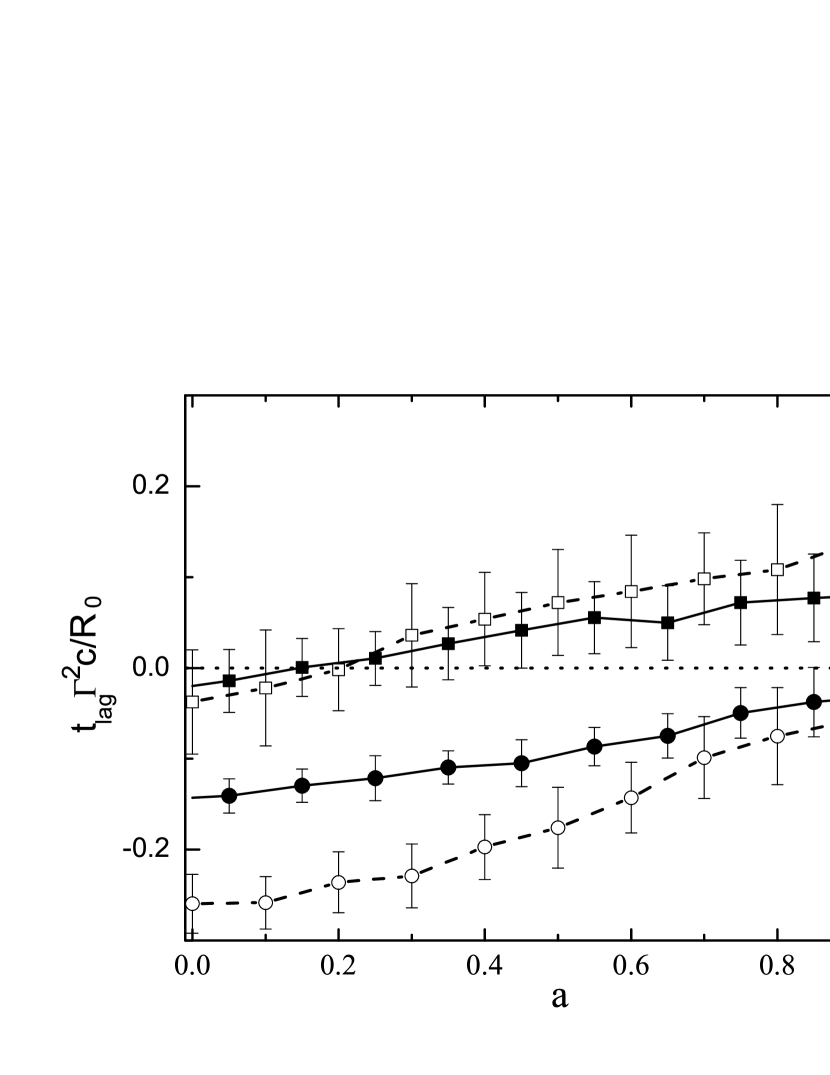
Figure 4: Lead/lag of the gamma-ray emission with respect to the observed synchrotron emission for different $|\mu^{\prime}|$ conditions. The empty symbols are for $f=0.8$ and the filled symbols are for $f=0.6$. The squares represent the numerical results with $|\mu^{\prime}|\geqslant a$, and the circles represent the results with $|\mu^{\prime}|\leqslant a$.

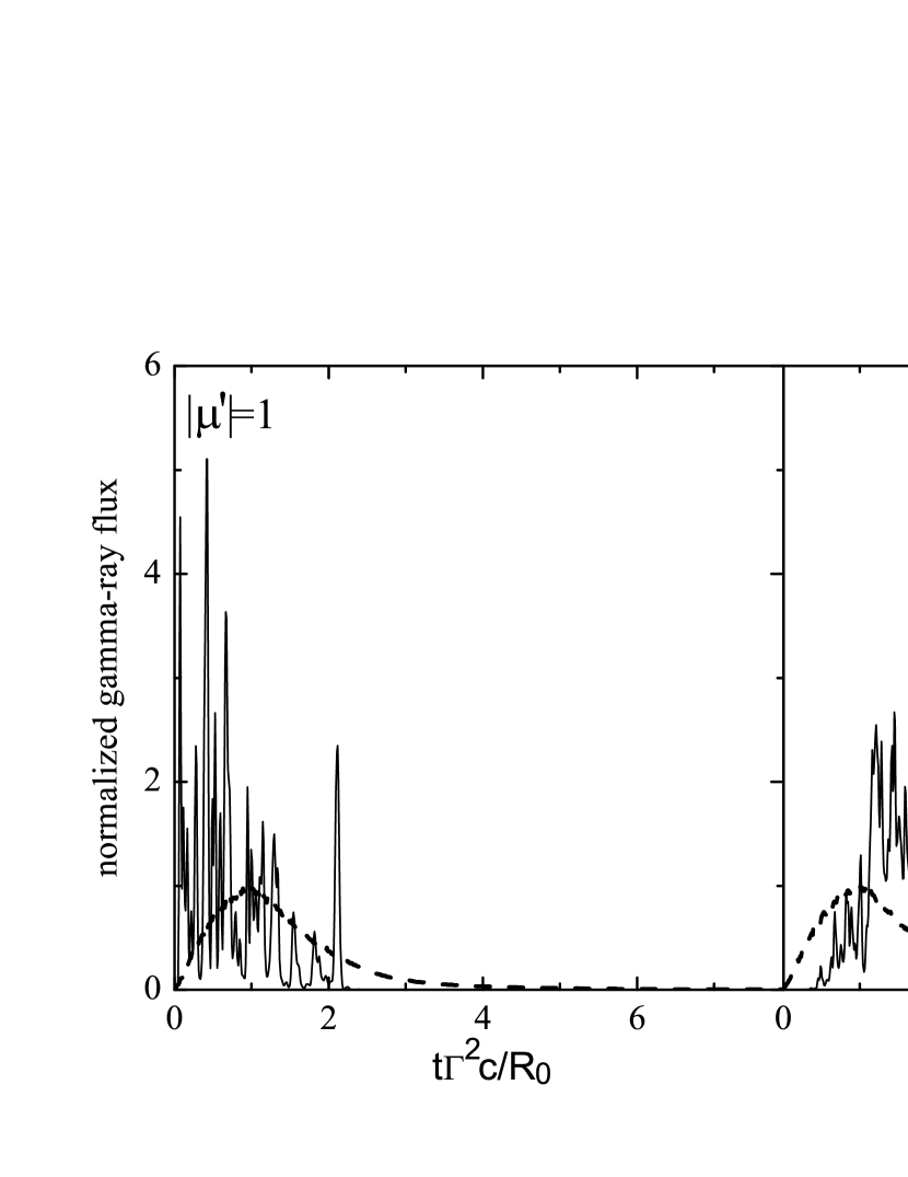
Figure 5: Two examples of light curves with $f=0.8$, where the solid curves correspond to the gamma-ray emission from eddies and the dashed lines correspond to the gamma-ray emission from inter-eddies. The left panel is for $|\mu^{\prime}|=1$, which shows that the peak time of gamma-ray emission from eddies is ahead of that from inter-eddies. The right panel is for $|\mu^{\prime}|=0$, which shows the opposite behavior.

References

- Ackermann et al. (2012) Ackermann, M., et al. 2012, ApJ, 754, 121
- Ackermann et al. (2013) Ackermann, M., et al. 2013, arXiv:1303.2908
- Beniamini et al. (2011) Beniamini, P., Guetta, D., Nakar, E., & Piran, T. 2011, MNRAS, 416, 3089
- Beskin et al. (2010) Beskin, G., Karpov, S., Bondar, S., et al. 2010, ApJ, 719, L10
- Daigne & Mochkovitch (1998) Daigne, F., & Mochkovitch, R. 1998, MNRAS, 296, 275
- Dermer & Mitman (1999) Dermer, C. D., & Mitman, K. E. 1999, ApJ, 513, L5
- Dichiara et al. (2013) Dichiara, S., Guidorzi, C., Amati, L., & Frontera, F. 2013, MNRAS, 431, 3608
- Fishman & Meegan (1995) Fishman, G. J., & Meegan, C. A. 1995, ARA&A, 33, 415
- Gao et al. (2012) Gao, H., Zhang, B.-B., & Zhang, B. 2012, ApJ, 748, 134
- Giannios et al. (2009) Giannios, D., Uzdensky, D. A., & Begelman, M. C. 2009, MNRAS, 395, L29
- Guetta et al. (2011) Guetta, D., Pian, E., & Waxman, E. 2011, A&A, 525, A53
- Katz (1994) Katz, J. I. 1994, ApJ, 422, 248
- Kobayashi et al. (1997) Kobayashi, S., Piran, T., & Sari, R. 1997, ApJ, 490, 92
- Kumar & Narayan (2009) Kumar, P., & Narayan, R. 2009, MNRAS, 395, 472
- Lazar et al. (2009) Lazar, A., Nakar, E., & Piran, T. 2009, ApJ, 695, L10
- Lu et al. (2012) Lu, R.-J., Wei, J.-J., Liang, E.-W., et al. 2012, ApJ, 756, 112
- Lyutikov & Blandford (2003) Lyutikov, M., & Blandford, R. 2003, arXiv:astro-ph/0312347
- Maxham & Zhang (2009) Maxham, A., & Zhang, B. 2009, ApJ, 707, 1623
- Morsony et al. (2010) Morsony, B. J., Lazzati, D., & Begelman, M. C. 2010, ApJ, 723, 267
- Narayan & Kumar (2009) Narayan, R., & Kumar, P. 2009, MNRAS, 394, L117
- Norris et al. (1996) Norris, J., Nemiroff, R. J., Bonnell, J. T., et al. 1996, ApJ, 459, 393
- Patricelli et al. (2012) Patricelli, B., Bernardini, M. G., Bianco, C. L., et al. 2012, ApJ, 756, 16
- Piran et al. (1993) Piran, T., Shemi, A., & Narayan, R. 1993, MNRAS, 263, 861
- Rees & Mészáros (1994) Rees, M. J., & Mészáros, P. 1994, ApJ, 430, L93
- Sari & Piran (1997) Sari, R., & Piran, T. 1997, ApJ, 485, 270
- Woźniak et al. (2009) Woźniak, P. R., Vestrand, W. T., Panaitescu, A. D., et al. 2009, ApJ, 691, 495
- Zhang et al. (2007) Zhang, B., Liang, E., Page, K. L., et al. 2007, ApJ, 655, 989