Do Intermediate-Mass Black Holes Exist in Globular Clusters?

Abstract

The existence of intermediate-mass black holes (IMBHs) in globular clusters (GCs) remains a crucial problem. Searching IMBHs in GCs reveals a discrepancy between radio observations and dynamical modelings: the upper mass limits constrained by radio observations are systematically lower than that of dynamical modelings. One possibility for such a discrepancy is that, as we suggest in this work, there exist outflows in accretion flows. Our results indicate that, for most sources, current radio observations cannot rule out the possibility that IMBHs may exist in GCs. In addition, we adopt an $\dot{M}-L_{\rm R}$ relation to revisit this issue, which confirms the results obtained by the Fundamental Plane relation.

1 Introduction

Over the past decades, astronomers have suspected that there might be a population of intermediate-mass black holes (IMBHs), which connect the stellar-mass black holes and the supermassive black holes. On the observational side, accretion of IMBHs could be the energy source of some hyper-luminous X-ray sources (HLXs), e.g., the well-known HLX-1 (Farrell et al., 2009; Davis et al., 2011). On the theoretical side, IMBHs are expected to be formed in centers of globular clusters (GCs) (e.g. Miller & Hamilton, 2002). Some of these IMBHs can be perfect candidates of first black hole seeds which eventually grow up to be SMBHs via merge or accretion (Volonteri, 2012). Others, however, may survive today. It is meaningful to search IMBHs in GCs.

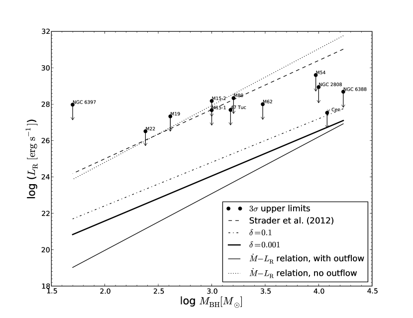
Figure 1: Radio luminosity $L_{\rm R}$ as a function of black hole mass $M_{\rm BH}$. The filled circles represent the $3\sigma$ upper limit of $L_{\rm R}$ for each source, where the black hole masses are constrained via dynamical modelings. The dashed line represents the predicted $L_{\rm R}$ as a function of $M_{\rm BH}$ according to Strader et al. (2012). The dot-dashed line and the thick solid line correspond to our new results with $\delta=0.1$ and $0.001$, respectively. The thin solid line and the dotted line represent $L_{\rm R}$ estimated by the $\dot{M}-L_{\rm R}$ relation instead of the Fundamental Plane relation with and without outflows, respectively.

One way to search IMBHs in GCs is to apply a dynamical modeling: model kinematic data of GCs. Many works have been done with this method (for the results of some GCs, see Table 1). These works suggested that GCs harbor IMBHs ($10^{2}\sim 10^{4}M_{\odot}$) in their centers. Another way to test the existence of IMBHs in GCs is to detect the unique signatures emitted by surrounding accretion flows. Unfortunately, the accretion rates to IMBHs (if IMBHs do exist) are expected to be extremely low since GCs have few gases. Therefore, it is quite difficult to directly detect X-ray emission. Maccarone (2004) suggested that radio observation could be a promising tool to probe IMBHs in GCs. The idea is based on the scenario that there exists a universal correlation among the X-ray luminosity ($L_{\rm{X}}$), the radio luminosity ($L_{\rm{R}}$), and the mass of black hole ($M_{\rm BH}$) (e.g., Merloni et al., 2003; Falcke et al., 2004; Wang et al., 2006; Plotkin et al., 2012, see also in Section 2.1). Basically, this so-called Fundamental Plane relation suggests that the radio/X-ray ratio increases with $M_{\rm BH}$. One can constrain the mass of an IMBH by using the Fundamental Plane relation, radio observations and the accretion theory (for the details, see Section 2). Also, the upper mass limits of IMBHs in GCs can be settled if radio observations do not detect any structures within the sensitivity of radio telescopes. Recently, Strader et al. (2012) obtained the $3\sigma$ upper limits of radio luminosity in three GCs (M15, M19, M22) with JVLA observations. Based on these data, they found that the corresponding upper limits of $M_{\rm BH}$ are too small for these GCs to harbor any IMBHs. Moreover, radio observations for other sources (see Table 1) also showed conflicts between the resulting upper limits of $M_{\rm BH}$ and the mass constrained via dynamical modelings (for details, see discussions in Strader et al., 2012, and our Figure 1). This discrepancy indicates that either IMBHs do not exist in GCs or the accretion onto IMBHs is significantly weaker than that predicted by the theory.

In this work, we take the role of outflows into consideration. As a consequence, the accretion rate onto IMBHs (and $L_{\rm R}$) will be significantly lower than what previously predicted. On the other hand, all sources in Table 1 seem to be in the quiescent state. The Fundamental Plane relation, as argued by Yuan & Cui (2005), should steepen into a new relation which differs from the one suggested by, for example, Merloni et al. (2003). Moreover, the Fundamental Plane relation, as mentioned by Plotkin et al. (2012), seems to indicate that the X-ray emission should originate from the jet rather than the ADAF. Considering that the X-ray luminosity in this work and some previous works is estimated by the ADAF solution, we therefore explore the validity of using the Fundamental Plane relation and the robustness of these results. The paper is organized as follows. In Section 2, we briefly summarize previous works on this issue. In Section 3, we compare our results with radio observations. Summary and discussion are given in Section 4.

2 Methods in previous works

In this section, we will discuss physics of constraining mass of IMBHs from radio observations in a detailed way (see also, Maccarone, 2004). The first step is on the calculation of $\dot{M}$. Previous works usually assume that the accretion rate is a fraction of Bondi accretion rate, i.e., $\dot{M}=f\dot{M}_{\rm{B}}$ (e.g., in Strader et al., 2012, $f=0.03$). The Bondi accretion is the spherical accretion starting from the Bondi radius $R_{\rm B}=2GM_{\rm BH}/c_{\rm s}^{2}(\infty)$, where $c_{\rm s}=(\gamma k_{\rm B}T/\mu m_{\rm{H}})^{1/2}$ is the speed of sound, and $\gamma$, $k_{\rm B}$, $T$ and $\mu$ are the ratio of specific heats, the Boltzmann constant, the temperature of gases and the mass per particle, respectively. Since the typical temperature of gases in GCs is around $T=10^{4}{\rm K}$, we have $R_{\rm B}\approx 10^{9}T_{4}^{-1}R_{\rm s}$, where $T_{4}=T/(10^{4}{\rm K})$, and $R_{\rm s}\equiv 2GM_{\rm BH}/c^{2}$ is the Schwarzschild radius. The corresponding Bondi accretion rate is (Frank et al., 2002)

$$\dot{M}_{\rm{B}}=(\frac{2}{5-3\gamma})^{\frac{5-3\gamma}{2(\gamma-1)}}\pi G^{2}M_{\rm BH}^{2}\frac{\rho(\infty)}{c_{\rm{s}}^{3}(\infty)}\ ,$$ (1)

where $\rho$ is the mass density of gases (in this work, we adopt $\rho=0.2m_{\rm H}$ cm^-3, $\gamma=1.4$, and $\mu=1.23$).

By knowing the accretion rate, one can now estimate $L_{\rm{X}}$ according to the accretion theory. The Eddington ratio of accretion rates is $\dot{m}\equiv\dot{M}/\dot{M}_{\rm Edd}\approx 4.3\times 10^{-5}fm_{2\rm k}$, where the Eddington rate is defined as $\dot{M}_{\rm Edd}=10L_{\rm Edd}/c^{2}$, and $m_{2\rm k}=M_{\rm BH}/(2000M_{\odot})$. Therefore, the flow should be an advection-dominated accretion flow (so-called “ADAF”). The corresponding radiative efficiency $\eta$ usually (although very roughly) scales as $\eta=0.1\dot{m}/\dot{m}_{\rm{c}}$, where near the IMBH $\dot{m}_{\rm{c}}\approx 0.01$ is the critical accretion rate of ADAFs. The bolometric luminosity is calculated by

$$L_{\rm{Bol}}=\eta\dot{M}c^{2}\ .$$ (2)

Previous works usually use $L_{\rm{X}}=L_{\rm{Bol}}$. Clearly, both of them are a function of the mass of IMBHs.

Since $L_{\rm{X}}$ scales as a function of $M_{\rm BH}$, one can obtain a one-to-one relation between $M_{\rm BH}$ and $L_{\rm R}$ by adopting the Fundamental Plane relation,

$$\log L_{\rm{X}}=A\log L_{\rm{R}}+B\log M_{\rm{BH}}+C\ ,$$ (3)

where $L_{\rm{X}}$ and $L_{\rm{R}}$ are both in units of $\rm erg~{}s^{-1}$, and $M_{\rm{BH}}$ is in units of the solar mass. The parameters $A$, $B$ and $C$ are constrained by observations. Equations (1)-(3) reveal that the non-detection of radio signals in GCs provide an upper limit of $M_{\rm{BH}}$.

However, attentions should be paid on this method. The first thing is about $\dot{M}$ near IMBHs, where most of energy is released. On one hand, since $\dot{m}_{\rm{c}}\sim 10^{-5}$ at $R_{\rm{B}}$ ($\dot{m}_{\rm{c}}$ scales as $\sim 0.01(r/10^{3})^{-1/2}$, see e.g., Narayan et al., 1998, where $r=R/R_{\rm{s}}$) and the angular momentum of gases in GCs is low, ADAFs are likely to extend to $R_{\rm{B}}$. When the angular momentum of gases in ADAFs is considered, the actual accretion rate at $R_{\rm B}$ is only a fraction of $\dot{M}_{\rm{B}}$, i.e., $\dot{M}(R_{\rm B})=\alpha\dot{M}_{\rm{B}}$ (Narayan et al., 1998), where $\alpha$ is the viscosity parameter. On the other hand, ADAFs are likely to suffer significant outflows (e.g., Quataert & Narayan, 1999; Li & Cao, 2009; Cao, 2010; Yuan et al., 2012). Following Yuan et al. (2012), outflows can be described by the following assumption:

$$\dot{M}=\alpha\dot{M}_{\rm B}(\frac{R}{R_{\rm out}})^{s}\ ,$$ (4)

where $R_{\rm out}$ is the outer radius of the ADAF. In this work we assume $R_{\rm{out}}=R_{\rm{B}}$. The parameter $s$, which determines the strength of outflows in ADAFs, cannot be self-determined by theoretical considerations. However, as pointed out by Yuan et al. (2012), some simulations (both hydrodynamical and magnetic-hydrodynamical) indicate $s=0.4\sim 0.5$ (observations of NGC 3115 also suggest $s\approx 0.4\sim 0.5$, see Wong et al., 2011). Therefore, the accretion rate near the IMBH is $\sim(10/R_{\rm{B}})^{0.4}\dot{M}_{\rm{out}}\sim 6\times 10^{-4}\alpha\dot{M}_{\rm{B}}$, which is smaller than that of Strader et al. (2012) (who assumed that $0.03\dot{M}_{\rm{B}}$ are accreted onto IMBHs).

Another thing is on the estimation of $\eta$, especially when ADAFs suffer outflows. Recently, Xie & Yuan (2012) have done a detailed calculation on $\eta$, which included the effects of outflows and found

$$\eta\equiv L_{\rm{Bol}}/\dot{M}_{\rm net}c^{2}=\eta_{0}(\frac{\dot{m}_{\rm net}}{\dot{m}_{\rm c}})^{\beta}\ ,$$ (5)

where $\dot{M}_{\rm net}$ is the accretion rate near the horizon of the black hole. The parameters $\eta_{0}$ and $\beta$ depend on the fraction of energy that directly heats electrons (denoted by $\delta$). For $\dot{m}$ less than $\sim 10^{-4}$ and $\delta=0.001~{}(0.1)$, Xie & Yuan (2012) shows $\eta_{0}=0.065~{}(0.12)$ and $\beta=0.71~{}(0.59)$.

As seen from Equation (3), $L_{\rm{R}}$ is sensitive to $L_{\rm{X}}$. The usually adopted $L_{\rm{X}}$ in fitting the Fundamental Plane relation is in the range of $1\sim 10$ keV (e.g. Merloni et al., 2003; Plotkin et al., 2012), which is only a fraction of the bolometric luminosity. This is because ADAF is optically thin and the spectrum is not a blackbody type but roughly a flat spectrum over $\sim 10$ orders of magnitude (from radio to hard X-ray) in the $\nu-\nu L_{\nu}$ diagram (e.g., Quataert & Narayan, 1999). It is therefore reasonable to assume

$$L_{\rm{X}}(1-10\ {\rm keV})=\zeta L_{\rm bol}\ ,$$ (6)

with $\zeta\sim 0.1$. In our opinion, $L_{\rm{X}}$ in some previous works is overestimated.

So far, we have argued that some modifications are required in determining mass of IMBHs by radio observations. In the following section, we will apply these modifications and present our results.

3 The existence of IMBHs in GCs

3.1 The predicted radio luminosity

Applying all the modifications discussed in Section 2, we can derive a new relation between $L_{\rm{R}}$ and $M_{\rm{BH}}$ with Equations (3)-(6) and the definition of $\dot{M}_{\rm{B}}$ (Equation 1),

$$\begin{split}\log L_{\rm{R}}&=\frac{38.05-3.30B-C-2.37\beta+\log(\zeta\eta_{0})}{A}\\ &+\frac{(\beta+1)\log(\lambda)}{A}+\frac{\beta+2-B}{A}\log(m_{2\rm{k}})\ ,\end{split}$$ (7)

where $\lambda=\alpha(R_{\rm{in}}/R_{\rm{B}})^{s}$ is the ratio between $\dot{M}_{\rm net}$ and $\dot{M}_{\rm{B}}$, and $R_{\rm{in}}$ is the inner radius of outflows. Following Yuan et al. (2012), we adopt $s=0.4$ and $R_{\rm{in}}=10R_{\rm{s}}$. We assume $\alpha=0.1$ and $\zeta=0.1$. For the Fundamental Plane relation, we adopt the one fitted by Plotkin et al. (2012), i.e., $A=1.45$, $B=-0.88$, and $C=-6.07$ (We choose this version of Fundamental Plane relation due to the following two reasons. First, the sample corresponding to this relation consists of sources with flat/inverted radio spectrum. When considering the radio observations of globular clusters, we usually assume a flat radio spectrum. Second, this sample, as pointed out by Plotkin et al., 2012, minimizes the systematical bias of synchrotron cooling and thus can be considered as the most robust relation.). As for $\delta$, we choose two typical values $\delta=0.1$ and $\delta=0.001$. Note that with $\lambda=0.03$, $\beta=1$, $\zeta=1$, and $\eta_{0}=0.1$, Equation (7) can recover the results of Strader et al. (2012).

Now, we can use Equation (7) to testify whether the recent radio non-detection results can rule out the existence of IMBHs in GCs or not. Table 1 lists the information of some GCs which may harbor IMBHs. $L_{\rm{R}}$ listed in Table 1 is the $3\sigma$ upper limit of radio luminosity constrained by radio observations. We calculate the predicted $L_{\rm{R}}$ for each source by using Equation (7) and mass listed in Table 1, and compare them with radio observations. The mass of IMBHs in Table 1 was obtained by dynamical modelings.

Figure 1 plots $L_{\rm R}$ as a function of $M_{\rm BH}$. As shown by Figure 1, $L_{\rm{R}}$ in our results are significantly lower than that of Strader et al. (2012). The major reason is relevant to outflows. The actual accretion rates near IMBHs are lower than that of Strader et al. (2012). More importantly, for most sources $L_{\rm{R}}$ in our results are obviously smaller than the $3\sigma$ upper limit of $L_{\rm{R}}$ given by radio observations. Thus, our results indicate that the current radio observations seem not to conflict with the dynamical modelings. In other words, IMBHs may still exist in GCs. An interesting exception is $\omega$ Cen. As seen from Figure 1, even in the presence of outflows, the predicted $L_{\rm{R}}$ is close to the $3\sigma$ upper limit of $L_{\rm{R}}$. Therefore, $\omega$ Cen is unlikely to harbor a $\sim 10^{4}M_{\odot}$ IMBH (see the last section for more details). In addition, the thin solid line and the dotted line in Figure 1 represents $L_{\rm R}$ estimated by the $\dot{M}-L_{\rm R}$ relation instead of the Fundamental Plane relation. We will interpret these results in the following subsection.

There are two issues we have to mention. The first issue is about the relatively large scatter in the Fundamental Plane relation. We will discuss this problem in the last section. The second one is the consistency of the assumptions that adopted in such an issue and previous works. The Fundamental Plane relation have been explored by many works. For instance, Yuan & Cui (2005) suggested that this relation can be explained in the framework that X-ray emission is predominantly from ADAFs whereas the radio emission is from jets. Moreover, they argued that in the extremely low luminosity region this relation should break into a new one. The argument is that, below a critical X-ray luminosity, $L_{\rm X,c}\approx 10^{-5}-10^{-6}L_{\rm Edd}$, the X-ray emission from the jet (radiatively cooled) should dominate over that from ADAFs (so-called “quiescent state”). In this spirit, all the sources in Table 1 should locate in this quiescent state. It seems more appropriate to use the Fundamental Plane relation obtained by Yuan & Cui (2005). Note that there are two Galactic black hole X-ray binaries (BHXRBs), A0620-00 (Gallo et al., 2006) and V404 Cyg (Corbel et al., 2008), whose X-ray luminosity is well below the critical X-ray luminosity proposed by Yuan & Cui (2005). The corresponding radio/X-ray correlation analyses are, however, inconsistent with the Fundamental Plane relation of Yuan & Cui (2005). In our opinion, there are two possibilities for these inconsistent results. The first one may be related to a large scatter in determining $L_{\rm X,c}$ (at least for V404), since $L_{\rm X,c}$ was constrained by assuming that there is a smooth transition of the Fundamental Plane relation from the type of Merloni et al. (2003) to that of Yuan & Cui (2005) at $L_{\rm X,c}$. Actually, if the Fundamental Plane relation of Plotkin et al. (2012) and that of Yuan et al. (2009) are used to constrain $L_{\rm X,c}$, one will find $L_{\rm X,c}\sim 10^{-7}L_{\rm Edd}$. The second possibility is related to the cooling of the jet. As mentioned by Yuan & Cui (2005), their Fundamental Plane relation is based on the assumption that the jet should be radiatively cooled in the X-ray bands. However, for the above two sources, such an assumption may be invalid due to the following reason. According to the synchrotron cooling frequency (under such circumstance, the Compton scattering can be neglected) $\nu_{\rm break}\propto m^{-1/2}\dot{m}^{-3/2}$ (e.g., Heinz, 2004), for low mass black holes and low accretion rates, the jet of the BHXRB may be uncooled.

On the other hand, at higher X-ray luminosity, the Fundamental Plane relation of Plotkin et al. (2012) indicates that the X-ray emission should be dominated by the synchrotron emission of the uncooled jet rather than the ADAF (see Figure 5 of Plotkin et al., 2012). Thus, both the arguments of Yuan & Cui (2005) and Plotkin et al. (2012) imply that the results of Section 3.1 (and the results of some previous works, e.g., Strader et al., 2012) would be suspicious according to the fact that the X-ray emission we considered in Section 3.1 is from ADAFs rather than jets. We will address this issue in the following subsection.

3.2 The influences of the Fundamental Plane relation and X-ray processes on the estimation of $M_{\rm{BH}}$ from $L_{\rm{R}}$

As stated in Section 3.1, there exists inconsistency between the Fundamental Plane relation we adopted and the radiative processes of X-ray emission we assumed. Then, it is natural to ask whether the results obtained in Section 3.1 will change significantly if we instead calculate the X-ray emission of the radiatively cooled jet and use the Fundamental Plane relation of Yuan & Cui (2005), or obtain the X-ray emission of the uncooled jet and use the Fundamental Plane relation of Plotkin et al. (2012). However, it is not easy to constrain the X-ray emission of the jet (whether cooled or uncooled) due to our poor knowledge of the jet physics. Therefore, we will investigate the issue in a different way, which is based on the idea that there may exist a correlation between $\dot{M}$ and the radio luminosity for flat spectrum radio cores (e.g., Blandford & Köumlnigl, 1979; Heinz & Sunyaev, 2003; Körding et al., 2006). The key point is whether this $\dot{M}-L_{\rm{R}}$ relation, as first quantitatively obtained by Körding et al. (2006) for low luminosity BHXRBs, depend on the origin of X-ray emission. If the sources whose X-ray emission is dominated by ADAFs share the similar relation with the sources whose X-ray emission mainly comes from jets, then one can expect that the results of Section 3.1 is robust. The physical reason is as follows. In Section 2, $L_{\rm{X}}$ is obtained by $L_{\rm{X}}=\zeta\eta\dot{M}_{\rm net}c^{2}$ (see Equation 6) rather than via X-ray observations. This equation and the Fundamental Plane relation actually reveal a direct relation between $\dot{M}$ and $L_{\rm{R}}$. In other words, Equation (7) is identical to an $\dot{M}-L_{\rm{R}}$ relation. Below, we will explore the $\dot{M}-L_{\rm{R}}$ relation of both ADAF-dominated and jet-dominated sources.

To answer this question, we search the literature for published information on $\dot{M}$ and $L_{\rm{R}}$. Our sample is collected from Wu et al. (2007)(seven FR I galaxies), Yuan et al. (2005)(XTE J1118+480), Yuan et al. (2009)(14 LLAGN) and Zhang et al. (2010)(three BHXBs) (see Table 2). Accretion rates of these sources are obtained by fitting the coupled ADAF-Jet model (for readers who are interested in details of this model, we recommend Yuan & Cui, 2005) to the overall spectral energy distribution (SED) of each source. Below we will try to summarize the main assumption of the coupled ADAF-Jet model.

The accretion flow is described by an ADAF with outflows (i.e., Equation 4). To fully account for the global solution of the ADAF, one should specify $\dot{M}_{\rm out}$, $R_{\rm out}$, $s$, the viscosity parameter $\alpha$, and the magnetic parameter $\beta$. The SED of the flow can be obtained after the global solution is solved (see e.g., Quataert & Narayan, 1999). On the other hand, the jet model is quantified based on the internal shock scenario used in gamma-ray burst models. In this model, a fixed fraction of material of the flow is lost into form a jet ($\dot{M}_{\rm jet}$). Other two parameters that quantify the geometry and motion of the jet are the half-opening angle $\phi$ and bulk Lorentz factor $\Gamma_{\rm jet}$. According to the internal shock scenario, shocks occur as shells with different velocity colliding with each other. As a consequence, a few fraction of electrons in the jet is accelerated into a power-law distribution (i.e., $N(E)\propto E^{-p}$, typically, $p\sim 2$). The remaining parameters are the fraction of accelerated electrons $\xi_{\rm e}$ and magnetic field in the shock front $\xi_{\rm B}$. With these parameters, one can calculate the SED of the jet by considering the synchrotron emission and/or Compton scattering. Note that the radiative cooling of the non-thermal electrons is also taken into consideration for the X-ray emission of the jet. Comparing the SED of coupled ADAF-Jet model with observations, one can, in principle, constrain $\dot{M}_{\rm out}$ (or $\dot{M}_{\rm jet}$ if X-ray emission is dominated by the jet), $R_{\rm out}$ (for an interesting discussion of the robustness of the obtained parameters, see Figures 4-6 of Zhang et al., 2010, which indicate that the calculated SED is inconsistent with data if $\dot{M}$ varies a little from the best fitting value). Besides, the origin of the X-ray emission can be found (indicated in Table 2).

We also include the data of BHXRBs used in Körding et al. (2006). These BHXRBs are under the state transition from the soft state to the hard state (except for GRS 1915+105, which is in a so-called “plateau state”). $\dot{M}$ can be calculated as $\dot{M}=L_{\rm X}/(0.1c^{2})$, where $c$ is the speed of light. Therefore, as shown by Table 2, we have 22 sources with X-ray emission dominated by the ADAF and nine sources with X-ray emission dominated by the jet. For the former 22 sources, we perform the OLS regression between $\dot{M}$ and $L_{\rm R}$. For the latter nine sources, however, both the X-ray emission and the radio emission are dominated by the jet, so the obtained $\dot{M}_{\rm out}$ is not reliable. We instead performed the OLS regression between $\dot{M}_{\rm jet}$ and $L_{\rm R}$. Our OLS regression results are presented in Table 3.

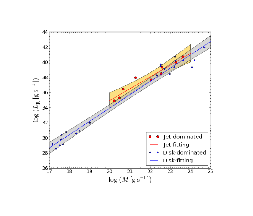
Figure 2: Relationship between accretion rate $\dot{M}$ and radio luminosity $L_{\rm R}$. The red circles (data) and the red line (fitting results) are for the sources whose X-ray emission is dominated by the ADAF. The blue stars (data) and the blue line (fitting results) correspond to the sources whose X-ray emission mainly comes from the jet. The filled regions are for the $2\sigma$ confidence bands of the fitting results.

As shown in Table 3, the slope of jet-dominated sources and ADAF-dominated sources are consistent with each other under $1\sigma$ uncertainties. However, it is inappropriate to directly compare the normalization of jet-dominated sources with that of ADAF-dominated ones because $\dot{M}_{\rm jet}$ is only a small fraction of $\dot{M}$. We assume $\dot{M}_{\rm jet}=f_{\rm jet}\dot{M}$ and choose a typical value $f_{\rm jet}=0.05$ to address this issue. By doing this, one can obtain an $\dot{M}-L_{\rm R}$ relation for the nine jet-dominated sources. We compare it with the one obtained from the ADAF-dominated ones. Figure 2 plots the results. As seen from this figure, the $\dot{M}-L_{\rm R}$ relation of jet-dominated sources is consistent with that of ADAF-dominated sources under $2\sigma$ uncertainties (filled regions in the plot). In order to further confirm our results, we have also tried to take the black hole mass into consideration, that is, we perform the OLS multivariate regression among $L_{\rm R}$, $\dot{M}$ ($\dot{M}_{\rm jet}$), and $M_{\rm BH}$. We find that the requirement of the parameter $M_{\rm BH}$ is statistically rejected under the $p$ value is 0.01. Thus, we can conclude that black holes in low activity state share a similar $\dot{M}-L_{\rm{R}}$ relation, regardless of $L_{\rm X}$ or the origin of the X-ray emission.

Since the $\dot{M}-L_{\rm{R}}$ relation does not depend on the origin of the X-ray emission, the results obtained in Section 3.1 are robust even if the X-ray emission may come from the synchrotron emission of the cooled Yuan & Cui (2005) or uncooled (Plotkin et al., 2012) jet. Other evidence that may confirm our conclusion is the thin solid line and the dotted line in Figure 1, which show $L_{\rm{R}}$ estimated by the $\dot{M}-L_{\rm{R}}$ relation (that is, the $\dot{M}-L_{\rm{R}}$ relation of the jet-dominated sources with, roughly, $L_{\rm{R}}\sim 10^{20}(\dot{M}_{\rm jet}/10^{9}\rm{g\ s^{-1}})^{1.56}\ \rm{erg\ s^{-1}}$ and $\dot{M}_{\rm jet}=0.05\dot{M}$, since X-ray emission of the sources in Table 1 may mainly come from the jet rather than the ADAF). For the case of Strader et al. (2012) ($\dot{M}=0.03\dot{M}_{\rm B}$, dotted line), the radio luminosity estimated from the $\dot{M}-L_{\rm R}$ is close to (within one order of magnitude) the radio luminosity obtained by assuming that the X-ray emission is dominated by the ADAF and using the Fundamental Plane relation (i.e., Section 3.1). The same conclusion holds (again within one order of magnitude) for our case (thin solid line).

4 Summary and Discussion

The radio observation is, as first demonstrated by Maccarone (2004), useful in probing IMBHs in GCs. However, the upper mass limits of IMBHs constrained by radio observations are significantly smaller than that of dynamical modelings. In this work, we showed that this inconsistency can be solved if ADAFs suffer outflows and IMBHs may exist in GCs. We also concluded that the results of Section 3.1 and previous works do not strongly depend on the physical processes of the X-ray emission and the type of Fundamental Plane relation, if $L_{\rm X}$ is obtained via the accretion theory.

The remaining question is about the scatter in the estimation. The Fundamental Plane relation of Plotkin et al. (2012) with $A=1.45$, $B=-0.88$ and $C=-6.07$ has a scatter of $\sigma_{\rm{int}}=0.07$. In this work, we have adopted this version of Fundamental Plane relation (for reasons, see Section 3.1). The uncertainty in estimating of $L_{\rm{X}}$ from $\dot{M}$ also contribute to the scatter. However, for almost all sources (except for $\omega$ Cen), the $3\sigma$ upper limits of radio luminosity are at least two orders of magnitude higher than that of our estimations. Therefore, the robustness of our conclusion that current radio observations cannot rule out the existence of IMBHs in GCs will not be affected by the above scatter.

$\omega$ Cen has long been considered as a promising source that may harbor an IMBH in its center. For example, the early work of Noyola et al. (2008) analyzed the HST ACS image and the Gemini GMOS-IFU kinematic data and concluded that $\omega$ Cen hosts an IMBH with $M_{\rm BH}=4.0^{0.75}_{-1.0}\times 10^{4}\ M_{\odot}$. However, van der Marel & Anderson (2010) explored a new dataset of HST proper motion and star count and given an upper limit of the mass of the IMBH in $\omega$ Cen: $M_{\rm BH}<1.2\times 10^{4}\ M_{\odot}$ at $1\sigma$ confidence (which is the value we adopted in this work). They also found that data can be well fitted with a $M_{\rm BH}=0.0$ model and the $M_{\rm BH}$ proposed by Noyola et al. (2008) is firmly ruled out, although the cluster center of van der Marel & Anderson (2010) is $\sim 12^{{}^{\prime\prime}}$ away from that of Noyola et al. (2008). Interestingly, Noyola et al. (2010) used the VLT-FLAMES to obtain the new data and found again that there should be an IMBH with $M_{\rm BH}\sim 5\times 10^{4}\ M_{\odot}$ in the center of $\omega$ Cen (note that even for the center of van der Marel & Anderson, 2010, they also concluded an IMBH with $M_{\rm BH}\sim 3\times 10^{4}\ M_{\odot}$). A recent work of Jalali et al. (2012) confirmed the conclusion of Noyola et al. (2010). In this work, $\omega$ Cen is the only one whose $3\sigma$ upper limit of $L_{\rm R}$ is close to the predicted radio luminosity even the outflows have been taken into consideration. To make the $\sim 4\times 10^{4}\ M_{\odot}$ IMBH compatible with the radio observations of $\omega$ Cen, one has to assume that the mass loss effect of outflows is larger than the one with $s=0.4$. Such an assumption challenges recent numerical simulations (e.g., Yuan et al., 2012) and observations (e.g., Wong et al., 2011). This leads us to conclude that the IMBH in $\omega$ Cen, if exists, is likely to be much lighter than $1.2\times 10^{4}\ M_{\odot}$, which is in agreement with van der Marel & Anderson (2010). More deep radio observations are required to draw robust conclusions.

Table 1: Recent Radio Observations of Globular Clusters

Sources	D (kpc)	log $L_{\rm R}$	Ref.	$M_{\rm dyn}(M_{\odot})$	Ref.
(1)	(2)	(3)	(4)	(5)	(6)
NGC 6388	13.2	28.684	1	$17000\pm 9000$	2
$\omega$ Cen	5.3	27.525	3	$<12000$	4
NGC 2808	9.5	28.940	5	$<10000$	6
M54	26.3	29.6	7	9400	8
M62	6.8	27.997	9	3000	9
M80	10	28.332	9	1600	9
47 Tur	4.5	27.684	3	$<1500$	10
M15(1)	10.3	27.672	11	1000	9
M15(2)	10.3	28.176	9	1000	9
M19	8.2	27.322	11	410	12
M22	3.2	26.505	11	240	12
NGC 6397	2.7	27.972	13	50	14

Col. (1): Name of Globular Cluster. Col. (2): Distance to the Sun (kpc). Col. (3) Logarithm of the center radio luminosity at 5 GHz ($3\sigma$ upper limit one, in units of $\rm{erg\ s^{-1}}$). Col. (5): Mass of Black Holes constrained by dynamical modelings.

REFERENCES: (1) Cseh et al. 2010; (2) Lützgendorf et al. 2011; (3) Lu & Kong 2011; (4) van der Marel & Anderson 2010; (5) Maccarone & Servillat 2008; (6) Lützgendorf et al. 2012; (7) Wrobel et al. 2011; (8) Ibata et al. 2009; (9) Bash et al. 2008; (10) McLaughlin et al. 2006; (11) Strader et al. 2012; (12) Maccarone 2004; (13) De Rijcke et al. 2006; (14) $M-\sigma$ relation of Tremaine et al. (2002).

NOTES: 1. There are two radio observations for M15. Here, M15(1) corresponds to Strader et al. (2012), and M15(2) corresponds to Bash et al. (2008). 2. For sources without mass uncertainties, there are absent of mass uncertainties in the referred paper.

Table 2: Radio Luminosity and Accretion Rate

Sources	log $\dot{M}$	log $L_{\rm R}$	$M_{\rm BH}(M_{\odot})$	$L_{2-10\rm keV}/L_{\rm Edd}$	Ref.	X-ray dominated by
(1)	(2)	(3)	(4)	(5)	(6)	(7)
IC 4296	23.197	39.329	$1.0\times 10^{9}$	$1.3\times 10^{-6}$	1	ADAF
NGC 315	23.249	40.181	$3.1\times 10^{8}$	$1.5\times 10^{-5}$	1	ADAF
NGC 1052	22.523	39.669	$1.26^{8}$	$5.9\times 10^{-6}$	1	ADAF
NGC 4203	22.324	38.314	$1.0\times 10^{7}$	$1.85\times 10^{-5}$	1	ADAF
NGC 4261	24.076	39.334	$4.9\times 10^{9}$	$4\times 10^{-6}$	1	ADAF
NGC 6251	24.189	40.258	$6\times 10^{8}$	$5\times 10^{-5}$	1	ADAF
NGC 4579	22.980	38.453	$4\times 10^{6}$	$3\times 10^{-4}$	1	ADAF
3C 346	24.680	41.900	$7.762\times 10^{8}$	$1.8\times 10^{-4}$	2	ADAF
3C 31	22.513	39.460	$7.762\times 10^{7}$	$4.4\times 10^{-6}$	2	ADAF
3C 317	23.225	40.730	$6.31\times 10^{8}$	$3.4\times 10^{-6}$	2	ADAF
B2 0055 +30	23.627	40.260	$1.514\times 10^{9}$	$2.4\times 10^{-6}$	2	ADAF
3C 449	22.712	39.080	$2.63\times 10^{8}$	$8.0\times 10^{-7}$	2	ADAF
XTE J1118 +480	17.509	28.977	8	$\sim 10^{-3}$	3	ADAF
Sw J1753.05 -0127	17.681	29.136	9	$\sim 5\times 10^{-3}$	4	ADAF
GRO J1655 -40	17.333	28.598	6.3	$\sim 10^{-3}$	4	ADAF
XTE J1720 -318	17.160	29.205	5	$\sim 2\times 10^{-3}$	4	ADAF
Cyg X-1	17.586	29.823	$14.8^{a}$	$\rm state\ transition^{f}$	5	ADAF
V404	17.624	30.408	$9.0^{b}$	$\rm state\ transition^{f}$	5	ADAF
GX 339-4(1)	17.846	30.776	$7.5^{c}$	$\rm state\ transition^{f}$	5	ADAF
1859+226	18.327	30.612	$>5.42^{d}$	$\rm state\ transition^{f}$	5	ADAF
GX 339-4(2)	18.506	30.939	$7.5^{c}$	$\rm state\ transition^{f}$	5	ADAF
GRS 1915+105	19.000	30.014	$10.1^{e}$	$\rm plateau\ state^{f}$	5	ADAF
IC 1459	21.286	39.319	$2.0\times 10^{9}$	$1.7\times 10^{-7}$	1	Jet
M81	19.365	36.446	$7.0\times 10^{7}$	$2.3\times 10^{-6}$	1	Jet
M84	21.247	38.483	$1.6\times 10^{9}$	$1.1\times 10^{-8}$	1	Jet
NGC 3998	19.976	37.930	$7.0\times 10^{8}$	$3\times 10^{-6}$	1	Jet
NGC 4594	20.742	37.668	$1.0\times 10^{9}$	$1.2\times 10^{-7}$	1	Jet
NGC 4621	19.173	35.288	$2.7\times 10^{8}$	$1.9\times 10^{-9}$	1	Jet
NGC 4697	18.914	34.877	$1.7\times 10^{8}$	$1\times 10^{-9}$	1	Jet
B2 0755 +3	22.313	40.720	$8.5\times 10^{8}$	$5.2\times 10^{-6}$	2	Jet
3C 66B	21.980	39.970	$6.9\times 10^{8}$	$1\times 10^{-6}$	2	Jet

REFERENCES: (1) Yuan et al. 2009; (2) Wu et al. 2007; (3) Yuan et al. 2005; (4) Zhang et al. 2010; (5) Körding et al. 2006.

NOTES: a. Mass adopted from Orosz et al. (2011); b. Mass adopted from Khargharia et al. (2010); c. Mass adopted from Chen (2011); d. Mass adopted from Corral-Santana et al. (2011); e. Mass adopted from Steeghs et al.(2013); f. Sources in the hard state but close to the state transition (GRS 1915 is in the radio plateau state); g. For the nine jet-dominated sources, $\dot{M}$ represents jet mass loss rate rather than accretion rate.

Table 3: The Fitting Results

X-ray emission dominated by	a	b	$p$ value
(1)	(2)	(3)	(4)
ADAF	$-15.42\pm 0.72$	$1.76\pm 0.06$	$<2.2\times 10^{-16}$
Jet	$-10.22\pm 1.78$	$1.56\pm 0.15$	$1.89\times 10^{-5}$

NOTES: 1. For sources whose X-ray emission is dominated by the ADAF, the fitting relation is $\log(L_{\rm R}/10^{30}\ \rm{erg\ s^{-1}})=a+b*\log(\dot{m}/10^{9}\ \rm{g\ s^{-1}})$; Otherwise, the fitting relation is $\log(L_{\rm R}/10^{30}\ \rm{erg\ s^{-1}})=a+b*\log(\dot{m}_{\rm jet}/10^{9}\ \rm{g\ s^{-1}})$.

References

- Bash et al. (2008) Bash, F. N., Gebhardt, K., Goss, W. M., & Vanden Bout, P. A. 2008, AJ, 135, 182
- Blandford & Köumlnigl (1979) Blandford, R. D., & Köumlnigl, A. 1979, ApJ, 232, 34
- Cao (2010) Cao, X. 2010, ApJ, 724, 855
- Chen (2011) Chen, T. 2011, IAU Symposium, 275, 327
- Corbel et al. (2008) Corbel, S., Koerding, E., & Kaaret, P. 2008, MNRAS, 389, 1697
- Corral-Santana et al. (2011) Corral-Santana, J. M., Casares, J., Shahbaz, T., et al. 2011, MNRAS, 413, L15
- Cseh et al. (2010) Cseh, D., Kaaret, P., Corbel, S., et al. 2010, MNRAS, 406, 1049
- Davis et al. (2011) Davis, S. W., Narayan, R., Zhu, Y., et al. 2011, ApJ, 734, 111
- de Rijcke et al. (2006) de Rijcke, S., Buyle, P., & Dejonghe, H. 2006, MNRAS, 368, L43
- Falcke et al. (2004) Falcke, H., Körding, E., & Markoff, S. 2004, A&A, 414, 895
- Farrell et al. (2009) Farrell, S. A., Webb, N. A., Barret, D., Godet, O., & Rodrigues, J. M. 2009, Nature, 460, 73
- Frank et al. (2002) Frank, J., King, A., & Raine, D. J. 2002, Accretion Power in Astrophysics, (3rd ed.; Cambridge: Cambridge Univ. Press)
- Gallo et al. (2006) Gallo, E., Fender, R. P., Miller-Jones, J. C. A., et al. 2006, MNRAS, 370, 1351
- Heinz (2004) Heinz, S. 2004, MNRAS, 355, 835
- Heinz & Sunyaev (2003) Heinz, S., & Sunyaev, R. A. 2003, MNRAS, 343, L59
- Hilburn & Liang (2012) Hilburn, G., & Liang, E. P. 2012, ApJ, 746, 87
- Ibata et al. (2009) Ibata, R., Bellazzini, M., Chapman, S. C., et al. 2009, ApJ, 699, L169
- Khargharia et al. (2010) Khargharia, J., Froning, C. S., & Robinson, E. L. 2010, ApJ, 716, 1105
- Körding et al. (2006) Körding, E. G., Fender, R. P., & Migliari, S. 2006, MNRAS, 369, 1451
- Jalali et al. (2012) Jalali, B., Baumgardt, H., Kissler-Patig, M., et al. 2012, A&A, 538, A19
- Li & Cao (2009) Li, S.-L., & Cao, X. 2009, MNRAS, 400, 1734
- Lützgendorf et al. (2012) Lützgendorf, N., Kissler-Patig, M., Gebhardt, K., et al. 2012, A&A, 542, A129
- Lützgendorf et al. (2011) Lützgendorf, N., Kissler-Patig, M., Noyola, E., et al. 2011, A&A, 533, A36
- Lu & Kong (2011) Lu, T.-N., & Kong, A. K. H. 2011, ApJ, 729, L25
- Maccarone (2004) Maccarone, T. J. 2004, MNRAS, 351, 1049
- Maccarone & Servillat (2008) Maccarone, T. J., & Servillat, M. 2008, MNRAS, 389, 379
- McLaughlin et al. (2006) McLaughlin, D. E., Anderson, J., Meylan, G., et al. 2006, ApJS, 166, 249
- Merloni et al. (2003) Merloni, A., Heinz, S., & di Matteo, T. 2003, MNRAS, 345, 1057
- Miller & Hamilton (2002) Miller, M. C., & Hamilton, D. P. 2002, MNRAS, 330, 232
- Narayan et al. (1998) Narayan, R., Mahadevan, R., & Quataert, E. 1998, in Theory of Black Hole Accretion Disks, ed. M. A. Abramowicz, G. Björnsson, & J. E. Pringle (Cambridge: Cambridge Univ. Press), 148
- Noyola et al. (2008) Noyola, E., Gebhardt, K., & Bergmann, M. 2008, ApJ, 676, 1008
- Noyola et al. (2010) Noyola, E., Gebhardt, K., Kissler-Patig, M., et al. 2010, ApJ, 719, L60
- Orosz et al. (2011) Orosz, J. A., McClintock, J. E., Aufdenberg, J. P., et al. 2011, ApJ, 742, 84
- Plotkin et al. (2012) Plotkin, R. M., Markoff, S., Kelly, B. C., Körding, E., & Anderson, S. F. 2012, MNRAS, 419, 267
- Quataert & Narayan (1999) Quataert, E., & Narayan, R. 1999, ApJ, 520, 298
- Steeghs et al. (2013) Steeghs, D., McClintock, J. E., Parsons, S. G., et al. 2013, ApJ, 768, 185
- Strader et al. (2012) Strader, J., Chomiuk, L., Maccarone, T. J., et al. 2012, ApJ, 750, L27
- Tremaine et al. (2002) Tremaine, S., Gebhardt, K., Bender, R., et al. 2002, ApJ, 574, 740
- van der Marel & Anderson (2010) van der Marel, R. P., & Anderson, J. 2010, ApJ, 710, 1063
- Volonteri (2012) Volonteri, M. 2012, Science, 337, 544
- Wang et al. (2006) Wang, R., Wu, X.-B., & Kong, M.-Z. 2006, ApJ, 645, 890
- Wong et al. (2011) Wong, K.-W., Irwin, J. A., Yukita, M., et al. 2011, ApJ, 736, L23
- Wrobel et al. (2011) Wrobel, J. M., Greene, J. E., & Ho, L. C. 2011, AJ, 142, 113
- Wu et al. (2007) Wu, Q., Yuan, F., & Cao, X. 2007, ApJ, 669, 96
- Xie & Yuan (2012) Xie, F.-G., & Yuan, F. 2012, MNRAS, 427, 1580
- Yuan & Cui (2005) Yuan, F., & Cui, W. 2005, ApJ, 629, 408
- Yuan et al. (2005) Yuan, F., Cui, W., & Narayan, R. 2005, ApJ, 620, 905
- Yuan et al. (2012) Yuan, F., Wu, M., & Bu, D. 2012, ApJ, 761, 129
- Yuan et al. (2009) Yuan, F., Yu, Z., & Ho, L. C. 2009, ApJ, 703, 1034
- Zhang et al. (2010) Zhang, H., Yuan, F., & Chaty, S. 2010, ApJ, 717, 929