Synthesis of the Conventional Phenomenological Theories of Superconductivity with Marginal Fermi Liquid Model

Abstract

In this work we have done phenomenology based model calculations for some of the thermodynamic and electrodynamic properties of the strongly correlated superconductors of Cuprate type. The method involves the application of the theoretical result for electronic specific heat in the normal phase from Marginal Fermi Liquid theory to the Gorter-Casimir two fluid model to derive the temperature dependence of the critical magnetic field corresponding to a type-I system, using the standard variational technique. We also applied this modified two fluid scheme to the London theory and obtained an expression for the temperature dependence of the magnetic field penetration depth in the superconducting phase. Our results are in fairly good agreement with other theoretical results based on different approaches, as well as with the experimental results.

1 Introduction

High temperature superconductivity in Cuprates has taken the centre stage of modern condensed matter physics since its discovery in 1987 because of the unusual normal state properties of these materials combined with the very rich phase diagram, besides the superconducting transition temperatures in the range of 40K-164K. These systems exhibit deviations from the Fermi liquid phenomenology in large regime of stoichiometric compositions. Moreover, the conventional microscopic theory is not always successful to explain the properties in the superconducting phase satisfactorily. On a phenomenological level, the behaviour below the optimal doping in the normal phase seems to display ‘marginal Fermi liquid’ (MFL) behaviour in the normal phase [19].
One of the most important features observed in experiments in the normal phase of the cuprates is the linear temperature dependence of dc resistivity, which below the optimal doping persists in an enormous temperature range from a few kelvin to much above room temperature.
The studies of the electrodynamic properties in the superconducting phase provide a clear phenomenological scenario, reveal information regarding the pairing state, the energy gap and the electronic density of states and thus provide important indications on the mechanism of high temperature superconductivity. A phenomenological model describing the marginal Fermi liquid behaviour of cuprates has been put forward by Varma and co-workers but its microscopic origin remains highly controversial. To our knowledge, no microscopic theory has so far been able to provide a satisfactory explanation for the phenomenon of high temperature superconductivity and anomalous normal phase properties of cuprates despite tremendous efforts during the last 3 decades [3].

Figure 1: Crystal structures of (a) $La_{2-x}Ba_{x}CuO_{4}$ and (b) $Nd_{2-x}Ce-xCuO_{4}$ superconductors

2 Gorter-Casimir Two Fluid Model

Gorter-Casimir two fluid model is an ’ad hoc’ model and it is based on two fundamental assumptions:

1. The superconducting state of a system is made up of two kinds of species viz. super-electrons and normal electrons. The perfectly ordered state occurs only at zero temperature and consists of super-electrons only and

2. The order parameter associated with the superconducting state is proportional to the number density of super-electrons and is dependent on temperature.

Let x represent the volume fraction of electrons belonging to the normal fluid and $1-x$, that belonging to the superfluid. Gorter and Casimir assumed the following formal analytical form for the free energy density of the electrons [22]:

$$F_{S}(x,T)=x^{\frac{1}{2}}f_{n}(T)+(1-x)f_{s}(T)$$ (1)

where

$$f_{n}(T)=-\frac{\gamma}{2}T^{2}$$ (2)

is the free energy density of the normal fluid and

$$f_{s}(T)=-\beta$$ (3)

is that for superfluid with $\gamma$ being the Sommerfeld constant and it is proportional to the single electron density of states per unit volume $N(0)$ at the Fermi and $\beta$ is an unknown parameter to be determined later. Minimizing the free energy density function $F(x,T)$ with respect to variations in $x$, one finds the equilibrium fraction of normal electrons at a temperature T.

$$\frac{\partial F(x,T)}{\partial x}=\frac{1}{2}x^{-{\frac{1}{2}}}f_{n}(T)-f_{s}(T)=0$$ (4)

At $T=T_{C}$, $x=1$
Thus we have

$$F_{n}=-2\beta\left(\frac{T}{T_{c}}\right)^{2}$$ (5)

and

$$F_{n}(T)-F_{s}(T)=\beta\left(1-\left(\frac{T}{T_{c}}\right)^{2}\right)^{2}$$ (6)

From the thermodynamic relation, it can be shown that

$$\frac{H_{c}^{2}(T)}{8\pi}=F_{N}(T)-F_{s}(T)$$ (7)

where $\frac{H_{c}^{2}(T)}{8\pi}$ is the stabilization (condensation) energy density of the pure superconducting state and $H_{c}\ (T)$ is the critical magnetic field. This leads to

$$H_{c}(T)=H_{o}\left(1-\left(\frac{T}{T_{c}}\right)^{2}\right)$$ (8)

where $H_{o}$ is the the critical magnetic field at zero temperature [6,7].

3 The London Theory

The brothers, H. London and F. London in 1935 [13] gave a phenomenological description of the electrodynamic properties of superconductors by proposing a scheme based on a two fluid type concept with super fluid and normal fluid densities $n_{s}$ and $n_{n}$ associated with velocities $v_{s}$ and $v_{n}$ respectively.The zero frequency penetration depth is a measure of the distance scale on which a static magnetic field will penetrate into a superconductor. Although the superconductor in the bulk has the property that it excludes all the magnetic flux, because of the superconducting screening current, it is in the surface layer that the field may still penetrate [19].
The first London equation is

$$\frac{\partial\bar{J}_{s}}{\partial t}=\frac{n_{s}e^{2}E}{m}$$ (9)

The second London equation is

$$\nabla\times\bar{J}_{s}=-\frac{n_{s}e^{2}}{mc}B$$ (10)

and the London penetration depth $\lambda_{L}$ is given as

$$\lambda_{L}=\left(\frac{mc^{2}}{4\pi n_{s}e^{2}}\right)^{\frac{1}{2}}$$ (11)

4 The BCS Theory

Bardeen, Cooper and Schrieffer (BCS) proposed a microscopic Hamiltonian for a superconductor, which is based on the idea of Cooper pairing [25]. Using this theory, they were able to successfully describe the interaction between electrons forming Cooper pair.

The BCS theory has a parameter $g$ defined as

$$g=N(o)V_{eff}$$ (12)

where $V_{eff}$ is the magnitude of the effective attractive interaction between the electrons forming a Cooper pair. From BCS equation in the weak coupling regime, one has the following equation for $T_{c}$

$$T_{c}=1.13\theta_{c}\exp\left(-\frac{1}{g}\right)$$ (13)

where $\theta_{c}$ is the temperature equivalent of the characteristic energy of the bosonic excitation mediating the pairing interaction. In the weak coupling regime, $0<g<0.25$.

Hereafter we would assume equation (13) to be valid even when the pairing is mediated by high energy electronic boson.

5 A Phenomenological Marginal Fermi Liquid Theory

In general, the unusual normal state properties of the high temperature superconducting copper-oxide compounds indicate a scattering rate for the itinerant electrons, that is linear in frequency $\omega$ and linear in temperature T over a large region. This implies that these materials can not satisfactorily be described by the conventional Fermi liquid picture.

Varma et al [20,22] postulated that in the copper oxide system, there are charge and spin density fluctuations of the electronic system, which are significantly distinct from those in the conventional Fermi Liquid. These two excitations however have similar behaviour. These fluctuations lead to a new contribution to the polarisability of the electronic medium that would renormalize the electron through the self energy in accordance with the observed scattering rates.
Their proposal for this contribution to the polarisability is as follows:

$$Im\ P(q,w)=\Bigg{\{}^{-N(0)\frac{w}{T},\qquad for\qquad|w|<T}_{-N(0)signw\qquad for\qquad|w|>T}$$ (14)

where N(0) is the single particle density of states at the Fermi energy [1].

Kuroda and Varma [3] calculated the specific heat of the marginal Fermi liquid in the normal phase using a Fermi liquid-like formula in the presence of electron-boson coupling constant. This boson is taken to be the itinerant particle-hole pair (exciton) itself in the normal state. They obtained the electronic specific heat $C_{v}$ of the marginal Fermi liquid as

$$C_{v}=N(0)\left(3+2\ln\frac{\theta_{c}}{T}\right)T$$ (15)

where $\theta_{c}$ is the characteristic temperature corresponding to the energy of the excitonic boson in the marginal Fermi liquid theory and assuming coupling coefficient $\lambda_{+}$=1.

6 Synthesis of Gorter-Casimir Two Fluid Model with Marginal Fermi Liquid Model

The free energy of conduction electrons in a metal is given by

$$f_{n}=U-T\displaystyle\int_{0}^{T}\dfrac{C_{v}(T)}{T}dT$$ (16)

where $\ U=\int_{0}^{T}C_{v}(T)dT$ and represents the internal energy of the electrons in the system.
We can then extend the above result and make use of Equation (15) to arrive at the following expression for the free energy density of the electrons in the normal phase of the marginal Fermi liquid:

$$f_{n}=-N(0)\left(3+\ln\frac{\theta_{c}}{T}\right)T^{2}$$ (17)

Making use of the two fluid model [see Equation (1)], the total electronic free energy density in the superconducting phase of the marginal Fermi liquid is now given as

$$F_{S}(x,T)=-x^{\frac{1}{2}}N(0)\left(3+\ln\frac{\theta_{c}}{T}\right)T^{2}\\ +(1-x)(-\beta)$$ (18)

$$\frac{\partial F(x,T)}{\partial x}=-\frac{1}{2}x^{-\frac{1}{2}}N(0)\left(3+\ln\frac{\theta_{c}}{T}\right)T^{2}\\ +\beta=0$$ (19)

This leads to the following equation after incorporating the expression for $\beta$ determined from the condition that for $T$ approaching $T_{c}$, $x$ approaches 1,

$$x=\left(\frac{3+\ln\frac{\theta_{c}}{T}}{3+\ln\frac{\theta_{c}}{T_{c}}}\right)^{2}\left(\frac{T}{T_{c}}\right)^{4}$$ (20)

where now $x$ represents the fraction of electrons in the normal fluid existing in the form of the marginal Fermi liquid.
Substituting the expression for $x$ from equation (20) into (18) gives

$$F_{S}(T)=-\frac{1}{2}N(0)\\ \times\left[\frac{\left(3+\ln\frac{\theta_{c}}{T}\right)^{2}}{\left(3+\ln\frac{\theta_{c}}{T_{c}}\right)}\frac{T^{4}}{{T_{c}}^{2}}+\left(3+\ln\frac{\theta_{c}}{T_{c}}\right)T_{c}^{2}\right]$$ (21)

Since $F_{N}(T)$=$f_{n}(T)$, it is given by equation (17) itself.
We recall that

$$C_{v}^{S}=-T\frac{\partial^{2}F_{s}(T)}{\partial T^{2}}$$

This yields,

$$C_{v}^{S}=N(0)\frac{T^{3}}{T_{c}^{2}}\frac{1}{\left(3+\ln\frac{\theta_{c}}{T_{c}}\right)}\\ \times\left[6\left(3+\ln\frac{\theta_{c}}{T}\right)^{2}-7\left(3+\ln\frac{\theta_{c}}{T}\right)+1\right]$$ (22)

Figure 2: Graph of specific heat in the superconducting phase $C_{v}$ against temperature T.

Also

$$C_{v}^{N}=N(0)\left(3+2\ln\frac{\theta_{c}}{T}\right)T$$ (23)

The difference between the specific heat capacity in the superconducting state $C_{v}^{S}$ and the specific heat capacity in the normal state $C_{v}^{N}$, called the specific heat jump $\triangle C_{v}$ is given as

$$\triangle C_{v}=C_{v}^{S}-C_{v}^{N}$$

At the critical temperature $\triangle C_{v}$ is given as

$$\triangle C_{v}|_{T=T_{c}}=N(0)T_{c}\frac{1}{\left(3+\ln\frac{\theta_{c}}{T_{c}}\right)}\\ \times\left[6\left(3+\ln\frac{\theta_{c}}{T_{c}}\right)-7+\frac{1}{\left(3+\ln\frac{\theta_{c}}{T_{c}}\right)}\right]\\ -N(0)\left(3+2\ln\frac{\theta_{c}}{T_{c}}\right)T_{c}$$ (24)

At critical temperature $T_{c}$, the ratio of the two types of specific heat is given as

$$\frac{C_{v}^{s}}{C_{v}^{N}}\bigg{|}_{T=T_{c}}=\frac{1}{\left(3+2\ln\frac{\theta_{c}}{T_{c}}\right)}\\ \times\left[6\left(3+\ln\frac{\theta_{c}}{T_{c}}\right)-7+\frac{1}{\left(3+\ln\frac{\theta_{c}}{T_{c}}\right)}\right]\\$$ (25)

The normalized specific heat jump at the transition temperature is given as

$$R=\frac{\triangle C_{v}}{C_{v}^{N}}\bigg{|}_{T=T_{c}}$$

and we have

$$R=\frac{1}{\left(3+2\ln\frac{\theta_{c}}{T_{c}}\right)}\\ \times\left[6\left(3+\ln\frac{\theta_{c}}{T_{c}}\right)-7+\frac{1}{\left(3+\ln\frac{\theta_{c}}{T_{c}}\right)}\right]-1$$ (26)

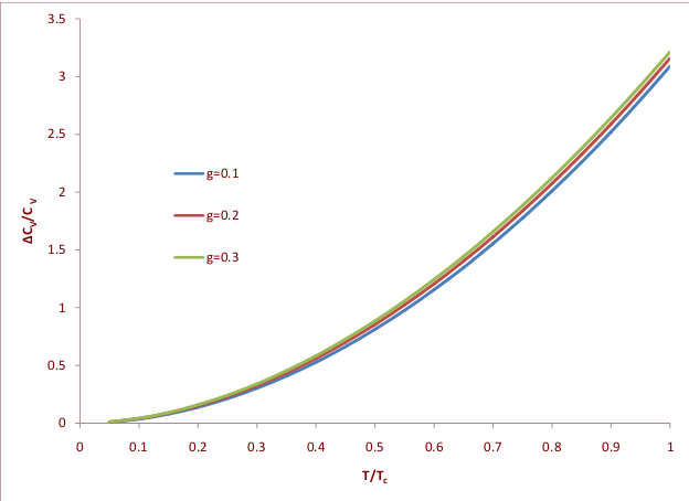
Figure 3: Graph of normalized specific heat jump in the superconducting phase $C_{v}$ against temperature $\frac{T}{T_{c}}$

At transition temperature, the normalized slope of the specific heat jump is given as

$$D=\frac{\frac{d(\triangle C_{v})}{dT}}{\frac{dC_{v}^{N}}{dT}}\bigg{|}_{T=T_{c}}$$

$$D=\frac{1}{\left(1+2\ln\frac{\theta_{c}}{T_{c}}\right)}\\ \times\left[18\left(3+\ln\frac{\theta_{c}}{T_{c}}\right)-33+\frac{10}{\left(3+\ln\frac{\theta_{c}}{T_{c}}\right)}\right]-1$$ (27)

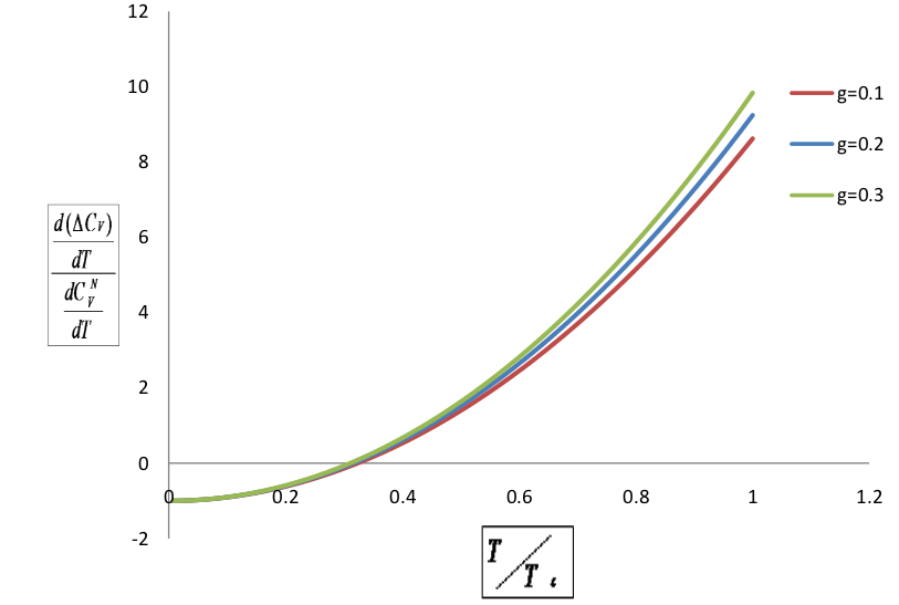
Figure 4: Graph of the normalized slope of specific heat jump in the superconducting phase $\Delta C_{v}$ against normalised temperature $\frac{T}{T_{c}}$

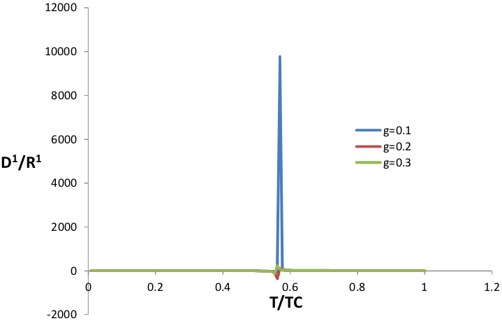
Figure 5: Graph of ratio of the normalized slope of specific heat jump and normalized specific heat jump in the superconducting phase $\frac{D}{R}$ against normalised temperature $\frac{T}{T_{c}}$

Making use of equations (17) and (23) in equation (7), we have

$$\frac{{H_{c}}^{2}(T)}{8\pi}=\beta\left[1-\left(\frac{3+\ln\frac{\theta_{c}}{T}}{3+\ln\frac{\theta_{c}}{T_{c}}}\right)\left(\frac{T}{T_{c}}\right)^{2}\right]^{2}$$ (28)

At $T=0$, $H_{c}(T)=H_{1}$ and we have

$$\frac{H_{1}^{2}}{8\pi}=\beta$$ (29)

and

$$H_{c}(T)=H_{1}\left[1-\left(\frac{3+\ln\frac{\theta_{c}}{T}}{3+\ln\frac{\theta_{c}}{T_{c}}}\right)\left(\frac{T}{T_{c}}\right)^{2}\right]$$ (30)

This is a departure from the conventional Two Fluid Model behaviour expected on the basis of the normal state modelled as a Fermi Liquid. From equation (13) we have

$$ln\left(\frac{\theta_{c}}{T_{c}}\right)=\frac{1}{g}-0.12$$

Equation (30) gives the expression for the temperature dependence of the critical magnetic for a superconductor arising from the marginal Fermi liquid normal phase.

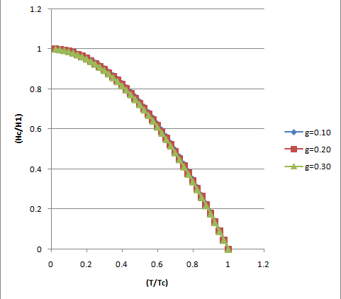
Figure 6: Graph $\frac{H_{c}}{H_{1}}$ against $\frac{T_{c}}{T}$ from equations (34(a)) and (39).

7 Synthesis of London Theory with MFL Model

From the two fluid model,

$$\frac{n_{s}}{n}=1-x$$ (31)

and we have

$$n_{s}=n\left[1-\left(\frac{3+\ln\frac{\theta_{c}}{T}}{3+\ln\frac{\theta_{c}}{T_{c}}}\right)^{2}\left(\frac{T}{T_{c}}\right)^{4}\right]$$ (32)

where $n_{s}$ and $n$ retain their meaning.
From London’s equations,

$$\lambda_{L}(T)=\left(\frac{mc^{2}}{4\pi n_{s}e^{2}}\right)^{\frac{1}{2}}$$ (33)

where $c$ is a constant and $m$ and $e$ are the mass and charge of electron
respectively.
At $T=0$, $n_{s}=n$ and the penetration depth $\lambda_{L}(T)$ becomes $\lambda_{L}(0)$ and we get

$$\lambda_{L}(0)=\left(\frac{mc^{2}}{4\pi ne^{2}}\right)^{\frac{1}{2}}$$ (34)

Substituting for $n_{s}$ in equation (32) into equation (33) gives

$$\lambda_{L}(T)=\frac{\lambda_{L}(0)}{\left[1-\left(\frac{3+\ln\frac{\theta_{c}}{T}}{3+\ln\frac{\theta_{c}}{T_{c}}}\right)^{2}\left(\frac{T}{T_{c}}\right)^{4}\right]^{\frac{1}{2}}}$$ (35)

where $\lambda_{L(0)}=\frac{c}{\omega_{p}}$. The temperature dependence shows departure from usual behaviour.

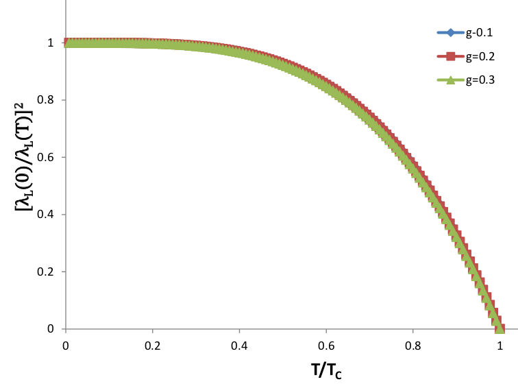
Figure 7: Graph of $\left[\frac{\lambda_{L}(0)}{\lambda_{L}(T)}\right]^{2}$ against $\frac{T}{T_{c}}$

8 Discussion of Results

In our model, we have incorporated the normal phase properties described by marginal Fermi liquid theory into the structure of Gorter-Casimir two fluid model. Specific heat measurements give information on the electron-boson coupling strength. The BCS theory and its subsequent refinements based on the Eliashberg equations show that high critical temperatures in superconductors are favoured by high values of the frequencies of the bosons mediating the pairing interaction and by the large electronic density of states at the Fermi level.

The quantity of interest is the difference between the electronic specific heats in the normal and superconducting phases. Our calculation shows that the normalized specific heat jump differs appreciably from $1.43$, the value corresponding to the BCS weak coupling limit for a superconducting transition from the conventional Fermi liquid phase.

At low temperatures, the lattice contribution to the total specific heat is small and can be accurately subtracted to extract the purely electronic contribution. The normal phase specific heat can be obtained by applying a magnetic field of sufficient strength to cause the sample to become normal.
The ratio of the normalized slope of specific heat jump and normalized specific heat jump in the superconducting phase $\frac{D}{R}$ at critical temperature $T_{c}$ is $4.1197$, $4.2616$, and $4.4110$ for $g=0.1,\ 0.2\ and\ 0.3$ respectively.
In the oxide superconductors, there are difficulties associated with these measurements. Because the superconducting critical temperatures of these oxide materials are relatively high, the lattice contribution to the total specific heat is quite large compared to the electronic contribution. An additional complication is that it is only possible to get normal state data close to critical temperature as the critical fields are quite large and are difficult to produce in the laboratory.

Figure (7) represents the experimental results for specific heat corresponding to YBCO. Comparing with figure $2$, observe that at low temperatures, there is an upturn in the specific heat rather than the expected exponential decay. However, there is still a linear term but there is no consensus yet on its origin. Analysis of the experimental data is usually done by assuming that the BCS relation $\frac{\triangle C}{\gamma T_{c}}=1.43$ holds. However it is pointed out by Beckman et al [27] that $\gamma$ extracted by this analysis is not in good agreement with values from high $T_{c}$ magnetization experiments and band structure calculations.

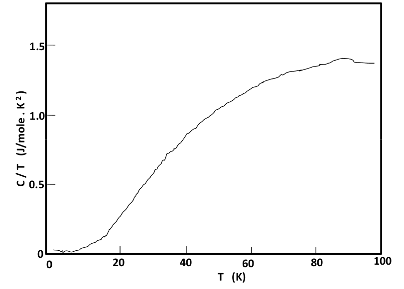
Figure 8: Experimental result for the specific heat of $YBa_{2}Cu_{3}O_{7}$.

Loram and Mirza [17] have used differential calorimetry on YBCO samples and report a normalized specific heat jump of $4.1$. Philips at al have reported a value of $4.8$.

From various observations, it would seem that there is a strong evidence for the specific heat jump to be large in the high $T_{c}$ materials. This large value of the normalized specific heat jump is consistent with the result of $\sim 3.02$ in the model of synthesizing the Gorter-Casimir two fluid model with marginal Fermi liquid theory as done in the BCS weak coupling regime this thesis.
In the second part of this work, we calculated the magnetic field penetration depth by applying the MFL modified two fluid model. The main aim was to investigate the effect of the charge and spin density fluctuations of the electronic system in the copper oxide materials. This we have done within the scope of the BCS weak coupling theory.

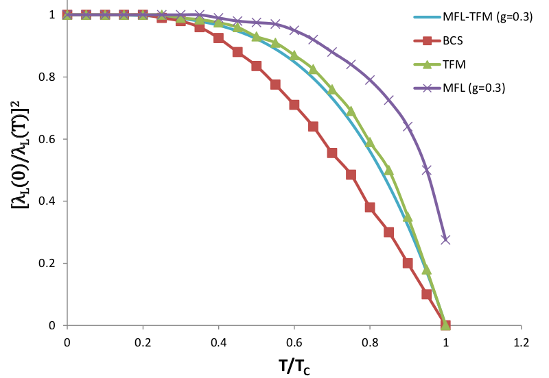
Figure 9: Comparism of the results of penetration depth from the BCS, TFM, MFL, and our calculation (TFM-MFL)

In figure (9) we have compared various results of the London penetration depth for the cuprate superconductor. The BCS weak coupling, the Gorter-Casimir two fluid model (TFM), the marginal Fermi liquid model (MFL) as done in the strong coupling regime by Nicol et al [19] and the synthesis of the MFL theory with London theory within the Two Fluid scheme (MFT-TFM) calculated in this piece of work. In general muon spin relaxation ($\mu$SR) experiments tend to agree more with the two fluid model. The most resent experimental result indicates temperature dependence conforming more to MFL-TFM like behaviour [28]
Note, however, that there is currently no consensus on the precise shape of $\frac{\lambda_{L}^{2}(0)}{\lambda_{L}^{2}(T)}$ in YBCO [15]

The London penetration depth from our result is close to the result of other results. If we extend our calculation to the BCS strong coupling regime, we hope to get a result closer to the experimental result.

9 Conclusion

In this research, we have applied the results from the marginal Fermi liquid theory to the $(i)$ Gorter-Casimir two fluid model and $(ii)$ London theory and used these to calculate some thermodynamic properties like the specific heat jump and the temperature dependence of the critical magnetic field. We also calculated the electrodynamic property in particular magnetic field penetration depth. The results of our calculations are closer to the experimental results obtained for Cuprates, than those from each of the phenomenological theories within the framework of ordinary Fermi liquid assumptions, independently.

In this study, we have only modified the normal fluid part of the Gorter-Casimir two fluid model. A more accurate result can be obtained by modifying the super fluid part as well. One method of doing this is to use a scheme based on many body formalism which leads to the free energy of the full superconducting phase for a MFL superconductor [3]. From this one can in principle subtract the normal fluid free energy density and thereby extract the super-fluid contribution corresponding to MFL.

Our methodology will be extended to a type-II superconducting system in future.

References

- [1] Abrahams, E, Littlewood, P. B, Ruckenstein, A. E, Schmitt-Rink, S,and Varma, C. M. Physical Review Letters, 63, 18, 1989.
- [2] Ashkroft, N. W and Mermin, N. D. Solid State Physics. New York: Holt, Rinehart and Winston, 1976.
- [3] Chaudhury Ranjan. Canadian Journal of Physics, 73, 1995.
- [4] Crisan, M and Moca, C. P. Journal of Superconductivity, 9, 1 1996.
- [5] Creswick, R, Farach, R. J, Poole, C. P, Prozorov, R. Superconductivity: Elsevier, 2007.
- [6] Gorter, C. J and H. G. B. Casimir. Phys. Z. 35, 963, 1934a.
- [7] Gorter, C. J and H. G. B. Casimir. Z. Tech. Phys. 15, 539, 1934b.
- [8] Halbritter J. Journal of applied physics 68, 6315, 1990.
- [9] Ketterson, J. B and Song, S. N. Superconductivity. Camdridge: Cambridge University Press, 1999.
- [10] Khomskii, D. I. Basic Aspects of the Quantum Theory of Solids: Order and Elementary Excitations. Cambridge: Cambridge University Press, 2010.
- [11] Kittel Charles. Introduction to Solid State Physics 5th Edition. New York: John Wiley and Sons Ltd., 1986.
- [12] Kostur, V. N and Radtke, R. J. Physical Review B. K. Levin, 1995͒.
- [13] London, F and H. London, H. Proc. Roy. Soc. A149, 71, 1935.
- [14] Mahan, G. D. Many-particle Physics Third Edition. New York: Kluwer Academic Plenum Publishers, 2000.
- [15] Mao, J et al. Phys. Rev. B 51, 3316, 1995͔͒.
- [16] Matsumoto Kaname General Theory of High-Tc Superconductors. Unpublished, 2010.
- [17] Mourachkine Andrei. Room-Temperature Superconductivity. United Kingdom: Cambridge International Science Publishing, 2004.
- [18] Muller, G and Peil, H. IEEE Transactions, Magnetics, 27, 854, 1991.
- [19] Nicol, E. J. Pair-Breaking in Superconductivity. Ph. D Thesis, McMaster University, 1991.
- [20] Nussinov, Z, van Saarloos, W and Varma, C. M. Singular or non-fermi liquids. Physics Reports, 361, 2002.
- [21] Parks, R. D. Superconductivity Vol. 2. New York: Marcel Dekker Inc, 1969.
- [22] Schofield, A. J. Non-Fermi liquids. Contemporary Physics 40, 1999.
- [23] Solymar, L and Walsh, D. Lectures on the Electrical Properties of Materials, 5th edition. New York: Oxford University Press, 1993.
- [24] Shoenberg, D. Superconductivity. London: Cambridge University Press, 1960.
- [25] Tinkham, M. Introduction to Superconductivity. New York: McGraw-Hill Inc, 1996.
- [26] Weinberg, S. The Quantum Theory of Fields Vol. II. London: Cambridge University Press, 1996.
- [27] Williams, P. J. Spin Fluctuations in Eliashberg Theory. Ph. D Theses, McMaster University, 1990.
- [28] Anlage, S. M et al. Preprint, 1991.