Effective slippage on superhydrophobic trapezoidal grooves

Abstract

We study the effective slippage on superhydrophobic grooves with trapezoidal cross-sections of various geometries (including the limiting cases of triangles and rectangular stripes), by using two complementary approaches. First, dissipative particle dynamics (DPD) simulations of a flow past such surfaces have been performed to validate an expression [E. S. Asmolov and O. I. Vinogradova, J. Fluid Mech. 706, 108 (2012)] that relates the eigenvalues of the effective slip-length tensor for one-dimensional textures. Second, we propose theoretical estimates for the effective slip length and calculate it numerically by solving the Stokes equation based on a collocation method. The comparison between the two approaches shows that they are in excellent agreement. Our results demonstrate that the effective slippage depends strongly on the area-averaged slip, the amplitude of the roughness, and on the fraction of solid in contact with the liquid. To interpret these results, we analyze flow singularities near slipping heterogeneities, and demonstrate that they inhibit the effective slip and enhance the anisotropy of the flow. Finally, we propose some guidelines to design optimal one-dimensional superhydrophobic surfaces, motivated by potential applications in microfluidics.

I Introduction

The design and fabrication of micro- and nanotextured surfaces has received much attention during the past decade. In case of a hydrophobic texture a modified surface profile can lead to a very large contact angle, which induces exceptional wetting properties Quere (2005). A remarkable mobility of liquids on such superhydrophobic surfaces is observed in the Cassie state, where the textures are filled with gas, which renders them “self-cleaning” and causes droplets to roll (rather than slide) under gravity Richard and Quere (1999) and rebound (rather than spread) upon impact Richard and Quere (2000); Tsai et al. (2010). Furthermore, patterned superhydrophobic materials are important in context of fluid dynamics and their superlubricating properties Vinogradova and Dubov (2012); McHale et al. (2010). In particular, superhydrophobic heterogeneous surfaces in the Cassie state exhibit very low friction, and this drag reduction is associated with the large slippage of liquids Bocquet and Barrat (2007); Rothstein (2010); Vinogradova and Belyaev (2011).

It is very difficult to quantify the flow past heterogeneous surfaces. However, analytical results can often be obtained using an effective slip boundary condition, $\mathbf{b}_{\mathrm{eff}}$, at the imaginary smooth homogeneous, but generally anisotropic surface Vinogradova and Belyaev (2011); Kamrin et al. (2010). For anisotropic textures, the effective slip generally depends on the direction of the flow and is a tensor, $\mathbf{b}_{\mathrm{eff}}\equiv\{b_{ij}^{\mathrm{eff}}\}$ represented by a symmetric, positive definite $2\times 2$ matrix Bazant and Vinogradova (2008)

$$\mathbf{b}_{\mathrm{eff}}=\mathbf{S}_{\theta}\left(\begin{array}[]{cc}b_{\mathrm{eff}}^{\parallel}&0\\ 0&b_{\mathrm{eff}}^{\perp}\end{array}\right)\mathbf{S}_{-\theta},$$ (1)

diagonalized by a rotation

$$\mathbf{S}_{\theta}=\left(\begin{array}[]{cc}\cos\theta&\sin\theta\\ -\sin\theta&\cos\theta\end{array}\right).$$ (2)

Equation (1) allows us to calculate an effective slip in any direction given by an angle $\theta$, provided the two eigenvalues of the slip-length tensor, $b_{\mathrm{eff}}^{\parallel}$ ($\theta=0$) and $b_{\mathrm{eff}}^{\perp}$ ($\theta=\pi/2$), are known. The concept of an effective slip length tensor is general and can be applied for arbitrary channel thickness Schmieschek et al. (2012). It is a global characteristic of a channel Vinogradova and Belyaev (2011), and the eigenvalues usually depend not only on the parameters of the heterogeneous surfaces, but also on the channel thickness. However, for a thick channel (compared to a texture period, $L$) they become a characteristic of a heterogeneous interface solely.

An important type of such surfaces are highly anisotropic textures, where a (scalar) partial local slip $b(y)$ varies in only one direction. Such surfaces can be created experimentally by making textured surfaces with one dimensional surface profiles, and in the Cassie state, the local slip length will always reflect the relief of the texture. This is the consequence of the “gas cushion model”, which takes into account that the dissipation at the gas/liquid interface is dominated by the shearing of a continuous gas layer Vinogradova (1995); Andrienko et al. (2003)

$$b(y)\simeq\frac{\mu}{\mu_{g}}e(y),$$ (3)

where $\mu_{g}$ and $\mu$ are dynamic viscosities of a gas and a liquid, and $e$ is the thickness of the gas layer. Eq. (3) represents an upper bound for a local slip at the gas area, which is attained in the limit of a small fraction of the solid phase. At a relatively large solid fraction Ybert et al. (2007) or if the flux in the “pockets” of superhydrophobic surfaces is equal to zero Maynes et al. (2007); Nizkaya et al. (2013), Eq. (3) could overestimate the local slip. However, even in all situations the local slip length profile, $b(y)$, necessarily follows the relief of the texture provided it is shallow enough, $e\left(y\right)\ll L$ Nizkaya et al. (2013). Since in case of water Eq. (3) leads to $b(y)\simeq 50e(y)$, it is expected that the “gas cushion model” could be safely applied up to $b(y)/L=O(10)$ or so.

The flow properties on highly anisotropic surfaces can be highly peculiar. In particular, off-diagonal effects may be obtained where a driving force (such as pressure gradient, shear rate, or electric field) in one direction induces a flow in a different direction, with a measurable and useful perpendicular component.This could be exploited for implementing transverse pumps, mixers, flow detectors, and more Stroock et al. (2002); Ajdari (2001). The main task is to find the connection between the eigenvalues of the slip-length tensor and the parameters of such one-dimensional surface textures. Up to now analytical results for the effective slip length have only been obtained for the simplest geometry of rectangular grooves Lauga and Stone (2003); Belyaev and Vinogradova (2010a); Ng et al. (2010); Zhou et al. (2012); Schmieschek et al. (2012); Asmolov et al. (2013a). We are unaware of any prior work that has obtained analytical results for other types of one-dimensional textures.

However, some recently derived relations for the case of an anisotropic isolated surface (corresponding to the thick channel limit) allow one to simplify the analysis of more complex geometries, and to rationalize the limiting behavior of the effective slip length in certain regimes. We mention first that the transverse component of the slip-length tensor was predicted to be exactly half the longitudinal component that one would obtain if the local slip were multiplied with a factor two, $2b(y)$ Asmolov and Vinogradova (2012)

$$b_{\mathrm{eff}}^{\bot}\left[b\left(y\right)/L\right]=\frac{b_{\mathrm{eff}}^{\parallel}\left[2b\left(y\right)/L\right]}{2}.$$ (4)

This relation can greatly simplify the analysis since it indicates that the flow along any direction of the one-dimensional surface can be easily determined, once the longitudinal component of the effective slip tensor is found. Equation (4) has been recently verified for a texture with sinusoidal superhydrophobic grooves by using a Lattice Boltzmann (LB) method Asmolov et al. (2013b), and for weakly slipping stripes by using dissipative particle dynamics (DPD) simulations Asmolov et al. (2013a).

Another useful relation addresses the particular case where the local slip is large, $b(y)/L\gg 1$. In that case, the effective slip length tensor $\textbf{b}_{\rm eff}$ becomes isotropic and is given by Asmolov et al. (2013b); Hendy and Lund (2007)

$$b^{\parallel}_{\rm eff}\simeq b^{\perp}_{\rm eff}\simeq\left\langle\frac{1}{b(y)}\right\rangle^{-1},$$ (5)

where $\left\langle 1/b(y)\right\rangle$ is the mean inverse local slip. Finally, for weakly slipping patterns with $b(y)/L\ll 1$, the flow again becomes isotropic, and its value is equal to the surface average of the local slip length Belyaev and Vinogradova (2010a); Kamrin et al. (2010):

$$b^{\parallel}_{\rm eff}\simeq b^{\perp}_{\rm eff}\simeq\langle b(y)\rangle=\langle b\rangle,$$ (6)

Note that Eq. (6) is expected to be accurate for a continuous local slip profile only. If the local slip length exhibits step-like jumps at the edges of heterogeneities, the expansions leading to Eq. (6) become questionable. Higher order contributions to the effective slip become comparable to the first-order term given by Eq. (6) and can no longer be ignored Asmolov et al. (2013a).

Computer simulations and numerical modeling can shed light on flow phenomena past one-dimensional surfaces. In efforts to better understand the connection between the parameters of the texture and the effective slip lengths, several groups have performed continuum and Molecular Dynamics simulations of flow past anisotropic surfaces. Most of these studies focused on calculating eigenvalues of the effective slip-length tensor for superhydrophobic stripes Cottin-Bizonne et al. (2004); Priezjev et al. (2005); Priezjev (2011). To study various aspects of a flow past striped walls, recent works employed Dissipative particle dynamics (DPD) Zhou et al. (2012); Asmolov et al. (2013a); Tretyakov and Müller (2013) and Lattice Boltzmann (LB) Schmieschek et al. (2012) methods. In the case of stripes with a piecewise constant local slip profile (i.e., the profile features steplike jumps at the boundaries of the stripes), the singularity in the slip profile induces singularities both in the pressure and velocity gradient, which generates an additional mechanism for dissipation even at small local slip Asmolov and Vinogradova (2012); Asmolov et al. (2013a). Anisotropic one-dimensional texture with continuously varying patterns can produce a very large effective slip. This has been confirmed in recent LB simulations studies of sinusoidal textures Asmolov et al. (2013b). One-dimensional continuous surfaces may also exhibit singularities (for example, the first derivative may be discontinuous). However, we are unaware of any previous work that has addressed the question of effective slip lengths past such textures.

In this paper we study the friction properties on trapezoidal superhydrophobic grooves [see Fig. 1(a)]. This texture is more general than rectangular grooves since it provides an additional geometrical structure parameter, i.e., the trapezoid base width. Also, the trapezoid texture can be extended to its extremes, such as a triangular patterns, where the liquid/solid contact area vanishes, and rectangular reliefs. Superhydrophobic trapezoidal textures were shown to give large contact angles, and to provide stable Cassie states Li et al. (2010). An obvious advantage of the trapezoidal surface relief is that the manufactured texture becomes mechanically more stable against bending compared to rectangular grooves. Furthermore, it can be naturally formed from dilute rectangular grooves as a result of elasto-capillarity Tanaka et al. (1993). This type of surfaces has already been intensively used in slippage experiments Choi et al. (2006). However, the impact of trapezoidal texture reliefs on transport and hydrodynamic slippage remains largely unknown.

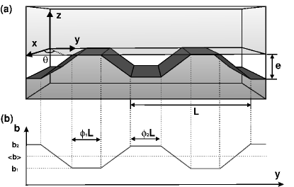
Figure 1: Sketch of the trapezoidal superhydrophobic surface in the Cassie state (a), and, according to Eq. (3), of the corresponding local slip length (b).

Our study is based on the use of DPD simulations, which we have put forward in our previous papers Zhou et al. (2012); Asmolov et al. (2013a), on the numerical solution of the Stokes equations (a collocation method), and on theoretical analysis. In particular, we validate Eq. (4) for trapezoidal textures with various parameters, we apply Eq. (5) to evaluate an effective slip for strongly slipping patterns, we discuss the singularities in velocities caused by inflection points in the local slip profiles, which in particular lead to deviations from Eq. (6), and we finally suggest the optimal design of trapezoidal patterns.

II Model and Governing Equations

We consider creeping flow along a plane anisotropic superhydrophobic wall, using a Cartesian coordinate system $(x,y,z)$ (Fig. 1). As in most previous publications Bocquet and Barrat (2007); Belyaev and Vinogradova (2010b); Priezjev et al. (2005); Lauga and Stone (2003); Ybert et al. (2007); Asmolov et al. (2011); Feuillebois et al. (2009); Schmieschek et al. (2012), we model the superhydrophobic plate as a flat heterogeneous interface. In such a description, we neglect an additional mechanism for a dissipation connected with the meniscus curvature Sbragaglia and Prosperetti (2007); Hyväluoma and Harting (2008); Ybert et al. (2007). Note however that such an ideal situation has been achieved in many recent experiments Steinberger et al. (2007); Karatay et al. (2013); Haase et al. (2013). The origin of coordinates is placed at the flat interface, characterized by a slip length $b(y)$, spatially varying in one direction, and the texture varies over a period $L$.

The local slip length is taken to be a piecewise linear function. It includes two regions with a constant slip: one where the slip length assumes its minimum value, $b_{1}$, which has area fraction of $\phi_{1}$, and another with area fraction $\phi_{2}$ where the slip length is maximal. These regions are connected by two transition regions with equal surface fractions $(1-\phi_{1}-\phi_{2})/2$, where the local slip length varies linearly from $b_{1}$ to $b_{2}$. If we rewrite the coordinate $y$ in the form $y=(n+t)L$, where $n$ is an integer number and $|t|\leq\frac{1}{2}$, the local slip-length profile can be expressed in terms of $t$:

$$b(y)=\begin{cases}b_{1},&|t|\leq\frac{\phi_{1}}{2}\\ b_{1}+\frac{2(b_{2}-b_{1})}{1-\phi_{1}-\phi_{2}}\big{(}|t|-\frac{\phi_{1}}{2}\big{)},&\frac{\phi_{1}}{2}<|t|\leq\frac{1-\phi_{2}}{2}\\ b_{2},&\frac{1-\phi_{2}}{2}<|t|\leq\frac{1}{2}\end{cases}$$ (7)

For $\phi_{1}=\phi_{2}=0$, we get a triangular profile

$$b(y)=b_{1}+2(b_{2}-b_{1})|t|,\quad|t|\leq\frac{1}{2}.$$ (8)

Note that regular trapezoidal and triangular profiles are continuous functions (albeit with a discontinuous first derivative). However, in the limit $\phi_{1}+\phi_{2}=1$, the profile reduces to the discontinuous rectangular slip length profile (alternating stripe profile) studied in earlier work

$$b(y)=\begin{cases}b_{1},&|t|\leq\frac{\phi_{1}}{2}\\ b_{2},&\frac{\phi_{1}}{2}<|t|\leq\frac{1}{2}\end{cases}$$ (9)

Our results apply to a single surface in a thick channel, where effective hydrodynamic slip is determined by flow at the scale of roughness, so that the velocity profile sufficiently far above the surface may be considered as a linear shear flow Bocquet and Barrat (2007); Vinogradova and Belyaev (2011). However it does not apply to a thin Feuillebois et al. (2009) or an arbitrary Schmieschek et al. (2012) channel situation, where the effective slip scales with the channel width. Note that the flow in thin channels with superhydrophobic trapezoidal textures has been considered in recent work Nizkaya et al. (2013).

Dimensionless variables are defined by using $L$ as a reference length scale, the inverse shear rate $1/G$ sufficiently far from the surface as a reference time scale, and setting the fluid kinematic viscosity, $\nu$, to unity (this sets the scale of mass). At small Reynolds number, $Re=GL^{2}/\nu,$ the dimensionless velocity and pressure fields, $\mathbf{v}$ and $p$, satisfy Stokes equations

$$\mathbf{\nabla}\cdot\mathbf{v}=0,$$ (10)

$$\mathbf{\nabla}p-\Delta\mathbf{v}=\mathbf{0}.$$

Due to Eq. (4), it is sufficient to consider the flow parallel to the pattern ($x$-axis). In this case, the velocity has only one component in the $x$-direction $\mathbf{v}=(v(y,z),0,0)$, and we seek a solution for the velocity profile of the form

$$v=U+u,$$ (11)

where $U=z$ is the undisturbed linear shear flow. The perturbation of the flow, $u(y,z)$, which is caused by the presence of the texture and decays far from the interface. It follows from Stokes’ equations that $\partial_{y}p=\partial_{z}p=0$. Since the pressure is constant far from the superhydrophobic surface this implies that it also remains constant in the entire flow region. The velocity perturbation satisfies a dimensionless Laplace equation

$$\Delta u=0.$$ (12)

The boundary conditions at the wall and at infinity are defined in the usual way

$$z=0: u-\frac{b(y)}{L}\partial_{z}u=\frac{b(y)}{L},$$ (13)

$$z\rightarrow\infty: \partial_{z}u=0.$$ (14)

The general solution to Eq. (12), decaying at infinity, can be represented in terms of a cosine Fourier series as

$$u=\frac{a^{0}}{2}+\sum_{n=1}^{\infty}a^{n}\exp(-2\pi nz)\cos(2\pi ny),$$ (15)

where $a^{n}$ are coefficients to be found by applying the appropriate boundary condition (13). It can be written in terms of the Fourier coefficients as

$$\frac{a^{0}}{2}+\sum_{n=1}^{\infty}\left[1+2\pi n\frac{b(y)}{L}\left(y\right)\right]a^{n}\cos\left(2\pi ny\right)=\frac{b(y)}{L}$$ (16)

Equation (16) was used to determine the longitudinal effective slip numerically. This was done using a method similar to Asmolov et al. (2013a). We truncate the sum in Eq. (16) at some cut-off number $N$ (usually $N=1001$) and evaluate it in the points $y_{l}=l/2\left(N-1\right),$ where $l$ are numbers varying from $0$ to $N-1$. The problem is then reduced to a linear system of equations, $A_{n}^{l}a^{n}L=b^{l},$ where $A_{0}^{l}=1/2$; $A_{n}^{l}=\left[1+2\pi nb\left(y_{l}\right)/L\right]\cos\left(2\pi ny_{l}\right)$, $n>0$ and $b^{l}=b\left(y_{l}\right).$ The system is solved using the IMSL routine LSARG. The transverse effective slip was then calculated using Eq. (4).

III Dissipative Particle Dynamics Simulation

Mesoscale fluid simulations were performed using the dissipative particle dynamics (DPD) method Hoogerbrugge and Koelman (1992); Español and Warren (1995); Groot and Warren (1997). More specifically, we use a version of DPD without conservative interactions Soddemann et al. (2003) and combine that with a tunable-slip method Smiatek et al. (2008) to model patterned surfaces. The tunable-slip method allows one to implement arbitrary hydrodynamic boundary condition in coarse-grained simulations. In the following, we give a brief description of the model and introduce the implementation of planar surfaces with arbitrary one-dimensional slip profile.

The basic DPD equations involve pair interactions between fluid particles. The pair forces are equal in magnitude but opposite in direction; thus the momentum is conserved for the whole system. This leads to the correct long-time hydrodynamic behavior (i.e. Navier-Stokes). The pair force consists of a dissipative contribution and a random component

$$\mathbf{F}_{ij}^{\rm DPD}=\mathbf{F}_{ij}^{\rm D}+\mathbf{F}_{ij}^{\rm R}.$$ (17)

The dissipative part $\mathbf{F}_{ij}^{\rm D}$ is proportional to the relative velocity between two particles $\mathbf{v}_{ij}=\mathbf{v}_{i}-\mathbf{v}_{j}$,

$$\mathbf{F}_{ij}^{\rm D}=-\gamma_{\rm DPD}\,\omega_{\rm D}(r_{ij})(\mathbf{v}_{ij}\cdot\hat{\mathbf{r}}_{ij})\hat{\mathbf{r}}_{ij},$$ (18)

with a local distance-dependent friction coefficient $\gamma_{\rm DPD}\omega_{\rm D}(r_{ij})$. The weight function $\omega_{\rm D}(r_{ij})$ is a monotonically decreasing function of $r_{ij}$ and vanishes at a given cutoff, and $\gamma_{\rm DPD}$ is a parameter that controls the strength of the dissipation. The random force $\mathbf{F}_{ij}^{\rm R}$ has the form

$$\mathbf{F}_{ij}^{\rm R}=\sqrt{2k_{B}T\gamma_{\rm DPD}\,\omega_{\rm D}(r_{ij})}\xi_{ij}\hat{\mathbf{r}}_{ij},$$ (19)

where $\xi_{ij}=\xi_{ji}$ is a symmetric random number with a zero mean and a unit variance. The amplitude of the stochastic contribution is related to the dissipative contribution by a fluctuation-dissipation theorem in order to ensure that the model reproduces the correct equilibrium distribution.

The tunable-slip method Smiatek et al. (2008) introduces the wall interaction in a similar fashion. The force exerted by the wall on particle $i$ is given by

$$\mathbf{F}_{i}^{\rm wall}=\mathbf{F}_{i}^{\rm WCA}+\mathbf{F}_{i}^{\rm D}+\mathbf{F}_{i}^{\rm R}.$$ (20)

The first term is a repulsive interaction that prevents the fluid particles from penetrating the wall. It can be written in term of the gradient of a Weeks-Chandler-Andersen potential Weeks et al. (1971):

$$\mathbf{F}_{i}^{\rm WCA}=-\nabla V(z),$$

$$V(z)=\left\{\begin{array}[]{cl}4\epsilon[(\frac{\sigma}{z})^{12}-(\frac{\sigma}{z})^{6}+\frac{1}{4}]&z<\sqrt[6]{2}\,\sigma\\ 0&z\geq\sqrt[6]{2}\,\sigma\end{array}\right.$$ (23)

where $z$ is the distance between the fluid particle and the wall, assuming the wall lies in $xy$ plane, and $\epsilon$ and $\sigma$ set the energy and length scales. In the following, physical quantities will be reported in a model unit system of $\sigma$ (length), $m$ (mass), and $\epsilon$ (energy). The dissipative contribution is similar to Eq. (18), with the velocity replaced by the relative particle velocity with respect to the wall. For immobile walls, the dissipative part can be written as

$$\mathbf{F}_{i}^{\rm D}=-\gamma_{\rm L}\omega_{\rm L}(z)\mathbf{v}_{i}.$$ (24)

The parameter $\gamma_{\rm L}$ characterizes the strength of the wall friction and can be used to tune the value of the slip length. For example, $\gamma_{\rm L}=0$ results in a perfectly slippery wall, whereas a positive value of $\gamma_{\rm L}$ leads to a finite slip length. The random force has the form

$$\mathbf{F}_{i}^{\rm R}=\sqrt{2k_{B}T\gamma_{\rm L}\omega_{\rm L}(z)}\boldsymbol{\xi}_{i},$$ (25)

where each component of $\boldsymbol{\xi}_{i}$ is a random variable. Again, the magnitude of the random force is chosen such that the fluctuation-dissipation theorem is satisfied.

Table 1: Parameters used in the DPD simulations.

fluid density $\rho$		$3.75\sigma^{-3}$
friction coefficient for DPD interaction $\gamma_{\rm DPD}$		$5.0\sqrt{m\epsilon}/\sigma$
cutoff for DPD interaction		1.0 $\sigma$
no-slip boundary condition $\gamma_{\rm L}$ ($b=0$)		$5.26\sqrt{m\epsilon}/\sigma$
cutoff for wall interaction		2.0 $\sigma$
dynamic viscosity $\mu$		$1.35\pm 0.01\sqrt{m\epsilon}/\sigma^{2}$
hydrodynamic boundary from the simulation wall		$1.06\pm 0.12\sigma$
simulation box		$20\sigma\times 40\sigma\times 82\sigma$
pattern period, $L$		$40\sigma$

For homogeneous surfaces, a useful analytical expression can be derived which establishes a relation between the slip length $b$ and the simulation parameters (the wall friction parameter $\gamma_{\rm L}$ and the cutoff $r_{c}$) to a good approximation Smiatek et al. (2008). However, the accuracy of the analytic result is not satisfactory at small slip lengths. For the purpose of the present work, we need an accurate expression for the relation between the slip length and the tuning parameter $\gamma_{\rm L}$. Therefore, we have simulated plane Poiseuille and Couette flows with different $\gamma_{\rm L}$ to obtain the slip length and the position of the hydrodynamic boundary. The simulation results were fitted to a truncated Laurent series up to second order in $\gamma_{\rm L}$ and first order in $1/\gamma_{\rm L}$. The simulation data and the fitted curve are shown in Fig. 2. The fit yields the expression

$$b=\frac{1.498}{\gamma_{\rm L}}-0.3291+0.01457\gamma_{\rm L}-0.001101\gamma_{\rm L}^{2}.$$ (26)

This formula relates the wall friction coefficient $\gamma_{\rm L}$, which is set in the simulation, to the slip length $b$. Also shown in Fig. 2 is the analytic result in dashed line, which agrees with the simulation data quite well at large slip length.

One important observation is that both the slip length $b$ and the friction coefficient $\gamma_{\rm L}$ are local quantities. Thus, it is reasonable to assume that the relation (26) also holds for inhomogeneous surfaces, as long as the slip length varies on length scales much larger than the range of the weight functions, $\omega_{\rm L}(z)$ and $\omega_{\rm D}(r)$. For a patterned surface with $L$ much larger than $\sigma$, the local friction coefficient $\gamma_{\rm L}(y)$ can be calculated from the slip profile $b(y)$ by inverting Eq. (26). The resulting profile $\gamma_{\rm L}(y)$ is then used in simulations to set up the patterned surfaces.

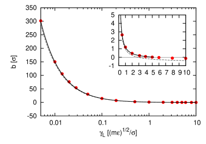
Figure 2: The relation between the slip length $b$ and the wall friction coefficient $\gamma_{\rm L}$, for a wall interaction cutoff $2.0\sigma$. The inset shows an enlarged portion of the region where the slip length is close to zero. The no-slip boundary condition is implemented by using $\gamma_{\rm L}=5.26\sqrt{m\epsilon}/\sigma$. The solid lines are the fitting result Eq. (26), and the dashed curves show the analytical prediction.

The simulations are carried out using the open source simulation package ESPResSo Limbach et al. (2006). Modifications have been made to incorporate the patterned surfaces. Table 1 summarizes the simulation parameters. In simulations, the patterned surface has a period of $L=40\sigma$. The simulation box is a rectangular cuboid of size $20\sigma\times 40\sigma\times 82\sigma$, periodic boundary conditions are assumed in the $xy$ plane, and the two symmetric patterned surfaces are located at $z=0\sigma$ and $z=82\sigma$. The separation between the two surfaces is about twice the pattern periodicity. We have checked that increasing the channel thickness does not change the results.

The simulation starts with randomly distributed particles inside the channel, and flow is induced by applying a body force to all particles. Body forces used in this simulation were chosen small enough that the flow velocity near the wall was less than $0.1\,\sqrt{\epsilon/m}$, in order to ensure that the flow is strictly laminar and effects of finite Reynolds numbers do not affect the simulation results. The magnitude of the slip velocity also affects the spatial resolution in modeling the variation of the slip length. Since the trajectories of the fluid particles are integrated at discrete time steps, the friction experienced by the particle between time steps is determined from the early instant. Therefore, we used a small time step of $0.01\sqrt{m/\epsilon}\sigma$. Due to the large system size, the relaxation time required for reaching a steady state was very large as well (over $10^{6}$ time steps). The flow velocity is small in comparison with the thermal fluctuation; thus many time steps are necessary to gather sufficient statistics. In this work, velocity profiles were averaged over $4\times 10^{5}$ time steps. A fit to the plane Poiseuille flow then gives the effective slip length $b_{\rm eff}$ Zhou et al. (2012). The error bars are obtained by six independent runs with different initialization.

Finally, we note that in case of a triangular local slip, only a very small region near the no-slip point contributes to the shear stress at large $b_{2}$. This presents a complication for simulations since fluid particles with a finite translational velocity travel a small distance over the no-slip region before reaching the zero averaged velocity. This distance is related to the initial velocity of the fluid particles when they enter the no-slip region, which is in general proportional to $b_{2}$ and the pressure gradient (the body force in simulation). To obtain accurate simulation data at large $b_{2}/L$, one has to reduce the body force significantly, and the necessary simulation times increase prohibitively. Therefore, only simulation results for $b_{2}/L=O(1)$ and smaller are presented for this texture.

IV Eigenvalues of the slip-length tensor

Here we present the results for the eigenvalues of the slip-length tensor obtained by simulations of different local slip profiles. We first verify Eq. (4), derived earlier by some of us Asmolov and Vinogradova (2012) to relate the longitudinal and transverse effective slip lengths. We use local slip profiles with $\phi_{1}=\phi_{2}$. In that special case, the profile $b(y)$ can be characterized by three parameters: the area fraction $\phi_{1}$ of the no-slip region, the surface-averaged slip length $\langle b\rangle=(b_{1}+b_{2})/2$, and the heterogeneity factor, $\alpha$, which is a measure for the relative variation of the slip length and defined as

$$\alpha=\frac{b_{2}-b_{1}}{2\langle b\rangle}=\frac{b_{2}-b_{1}}{b_{2}+b_{1}}$$ (27)

A homogeneous surface then corresponds to $\alpha=0$, and low values of $\alpha$ corresponds to small $b_{2}/b_{1}$. Patterns involving no-slip regions, (i.e. $b_{1}=0$) have $\alpha=1$. Such a no-slip assumption can be justified provided $b_{2}/b_{1}\gg 1$, which is typical for many situations. Indeed, for most smooth hydrophobic surfaces, the slip length is of the order of a few tens of nm Vinogradova and Yakubov (2003); Vinogradova et al. (2009); Cottin-Bizonne et al. (2005); Joly et al. (2006), which is very small compared to the slip length values of up to tens or even hundreds of $\mu$m slip lengths that may be obtained on the gas areas.

IV.1 Fixed average slip

Let us first investigate the effect of $\alpha$ on the effective slip at fixed $\langle b\rangle/L=0.5$. Figure 3(a) shows the simulation results for eigenvalues of the slip length tensor as a function of $\alpha$ obtained for a trapezoidal local slip ($\phi_{1}=0.25$). Also included are numerical results (solid curves) calculated with Eqs. (4) and (16). The agreement between the simulation and numerical results is quite good for all $\alpha$. This demonstrates both the accuracy of our simulations, and the validity of Eq. (4). The data presented in Fig. 3(a) show that the longitudinal slip is larger than the transverse slip, i.e., the flow is anisotropic, and the anisotropy increases with $\alpha$. The effective slip assumes its maximum value at $\alpha=0$, when the surface is homogeneous, and then decreases monotonously. This implies that the effective slip is found to be always smaller than the surface-averaged value, and the difference from the average value increases with the heterogeneity. A similar behavior was reported in prior work for other types of patterns Vinogradova (1999); Asmolov et al. (2013b). In the case of large local slip, the effective slip length can be obtained from Eq. (5), which gives for a trapezoidal slip profile, Eq. (7):

$$b_{\mathrm{eff}}\simeq\left[\frac{\phi_{1}}{b_{1}}+\frac{\phi_{2}}{b_{2}}+\frac{1-\phi_{1}-\phi_{2}}{2\left(b_{2}-b_{1}\right)}\ln\left(\frac{b_{2}}{b_{1}}\right)\right]^{-1}.$$ (28)

Figure 3(a) includes the theoretical curve expected for this (isotropic) case (dash-dotted line). We note that the slip length is always smaller than the average slip, $\langle b\rangle/L=0.5$. Perhaps the most interesting and important result here is that Eq. (28) remains surprisingly accurate even in the case of moderate, but not vanishing, local slip, provided $\alpha$ is small enough. We remind the reader that Eq. (28) may not be used when $\alpha=1$, i.e., for textures with no-slip regions, $b_{1}=0$, where it would simply predicts the effective slip length to be zero.

Qualitatively similar results were obtained for rectangular stripes and triangular local slip profiles. Therefore we do not show these results here. We only recall that in the case of stripes, the asymptotic result for large slip gives (see Asmolov et al. (2013b); Cottin-Bizonne et al. (2004) for the original derivations),

$$b_{\mathrm{eff}}\simeq\left[\frac{\phi_{1}}{b_{1}}+\frac{\phi_{2}}{b_{2}}\right]^{-1},$$ (29)

and for triangular profiles, one can derive

$$b_{\mathrm{eff}}\simeq\frac{2(b_{2}-b_{1})}{\ln(b_{2}/b_{1})}.$$ (30)

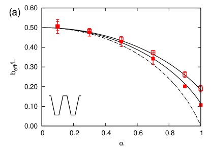
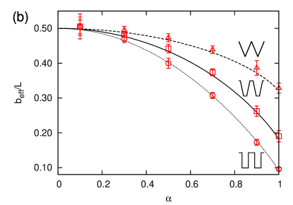
Figure 3: (a) Longitudinal (open symbols) and transverse (closed symbols) effective slip for a trapezoidal texture with an average slip $\langle b\rangle/L=0.5$. Solid curves show corresponding numerical solutions. Dash-dotted curve shows asymptotic solution in the limit of the large local slip [Eq. (28)]. (b) Longitudinal effective slip length simulated (from top to bottom) for triangular, trapezoidal, and rectangular profiles with the same average slip $\langle b\rangle/L=0.5$ (symbols) and corresponding numerical data.

To examine the difference between the different slip profiles, the results for a longitudinal effective slip for a texture with a trapezoidal local slip from Fig. 3(a) are reproduced in Fig. 3(b). Also included in Fig. 3(b) are numerical and simulation data for rectangular ($\phi_{1}=0.5$) and triangular ($\phi_{1}=0$) profiles with the same average slip. The data show that the triangular profile gives a larger, and the rectangular one a smaller effective slip than that resulting from the trapezoidal local slip. We note that $\phi_{1}$ is very different for these slip-length profiles. This suggests that one of the key parameters determining the effective slip is the area fraction of solid in contact with the liquid. If it is very small, the effective slip length becomes large. Another important factor is the presence of flow singularities near slipping heterogeneities as we will discuss below.

IV.2 Fixed heterogeneity factor

We now fix $\alpha=1$ and consider flows that are maximally anisotropic for a given pattern, which corresponds to $b_{1}=0$ (no-slip areas) and $b_{2}=2\langle b\rangle$. It is instructive to focus first on the role of $b_{2}$. Fig. 4 shows the eigenvalues of the slip-length tensor as a function of $b_{2}/L$ as obtained from simulations (symbols). As before we include numerical results (solid curves) calculated with Eqs. (4) and (16). We remind that the “gas cushion model”, Eq. (3), becomes very approximate at $b_{2}/L\gg 1$, and the local slip profile could not necessarily follow the relief of the texture. It is, however, instructive to include large values of $b_{2}/L$ into our consideration below since this will provide us with some guidance.

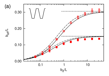
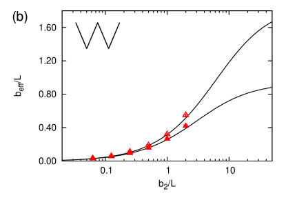
Figure 4: Effective slip lengths as a function of $b_{2}/L$ at $\alpha=1$ for (a) trapezoidal and (b) triangular local slip. Symbols show simulation data for longitudinal (open) and transverse (closed) effective slip lengths. The solid curves are results of numerical solutions. Dash-dotted curves show the predictions of analytic formulae [Eqs. (31, 32)] for stripes with the same fraction of no-slip areas. Dashed lines show the asymptotic values for stripes at large $b_{2}/L$ [Eq. (33)].

The eigenvalues of the slip-length tensor for a superhydrophobic trapezoidal texture are shown in Fig. 4(a). The agreement between the theoretical and simulation data is very good for all $b_{2}/L$, again confirming the accuracy of the simulations and the validity of Eq. (4). Qualitatively, the results are similar to those obtained earlier for a striped surfaces Belyaev and Vinogradova (2010a): At very small $b_{2}/L$, the effective slip is small and appears to be isotropic, in accordance to predictions of Eq. (6). It becomes anisotropic and increases for larger $b_{2}/L$, and saturates at $b_{2}/L\gg 1$. In case of stripes with alternating regions of no-slip ($b_{1}=0$) and partial-slip ($b_{2}=2\langle b\rangle$) areas the situation can be described by simple analytic formulae Belyaev and Vinogradova (2010a)

$$\frac{b_{\rm eff}^{\parallel}}{L} \simeq \frac{1}{\pi}\frac{\displaystyle\ln\left[\sec(\frac{\pi\phi_{2}}{2})\right]}{\displaystyle 1+\frac{L}{\pi b_{2}}\ln\left[\sec(\frac{\pi\phi_{2}}{2})+\tan(\frac{\pi\phi_{2}}{2})\right]},$$ (31)

$$\frac{b_{\rm eff}^{\perp}}{L} \simeq \frac{1}{2\pi}\frac{\displaystyle\ln\left[\sec(\frac{\pi\phi_{2}}{2})\right]}{\displaystyle 1+\frac{L}{2\pi b_{2}}\ln\left[\sec(\frac{\pi\phi_{2}}{2})+\tan(\frac{\pi\phi_{2}}{2})\right]}$$ (32)

In the limit of $b_{2}\gg L$, these expressions turn into those derived earlier for perfect slip stripes Philip (1972); Lauga and Stone (2003)

$$\frac{b_{\rm eff}^{\parallel}}{L}=\frac{2b_{\rm eff}^{\perp}}{L}\simeq\frac{1}{\pi}\ln\left[\sec\left(\frac{\pi\phi_{2}}{2}\right)\right].$$ (33)

For comparison, we plot the above expressions (using the value $\phi_{1}=0.25$ of the trapezoidal texture) in Fig. 4(a) as dash-dotted [Eqs. (31,32)] and dashed [Eq. (33] lines. One can see that with these parameters, the results for stripes practically coincides with those for trapezoidal slip at very small and very large $b_{2}/L$. At intermediate local slip there is a small discrepancy, suggesting that the equations for partial slip stripes overestimate the effective slip for trapezoidal texture. We will return to a discussion of these results later in the text.

Figure 4(b) plots the simulation results for a triangular local slip profile, which is particularly interesting since $\phi_{1}=0$. As explained above, simulation data could only be obtained for small values of $b_{2}$ in this case. In contrast, our numerical approach allowed us to calculate the effective slip length over a much larger interval of $b_{2}/L$. These numerically computed slip lengths are also included in Fig. 4(b). In the regime where simulation data are available, the agreement with the simulation and numerical results is excellent, therefore validating Eq.(4). It is interesting to note that according to the numerical calculations, the effective slip lengths grow weakly with $b_{2}/L$ at large $b_{2}/L$ and likely do not saturate, in contrast to rectangular and trapezoidal textures.

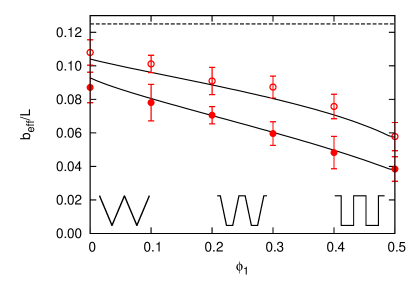
Figure 5: Effective slip lengths as functions of $\phi_{1}$ for surfaces with $\alpha=1$ and $\langle b\rangle/L=0.125$. The open and closed symbols are simulation results for the longitudinal and transverse effective slip lengths, respectively. Solid lines are numerical results. Dashed line shows predictions of Eq. (6).

Finally we compare the effective slip of surfaces with the same $\alpha$ and $\langle b\rangle/L$, but different $\phi_{1}$. Fig. 5 shows the corresponding curves for a maximal heterogeneity factor, ($\alpha=1$), and a relatively small $\langle b\rangle/L=0.125$. The results for larger $\langle b\rangle/L$ are qualitatively similar and not shown here. Only the values of the effective slip lengths become larger.) We note that by varying $\phi_{1}$ from 0 to 0.5, we change the local slip profile from triangular ($\phi_{1}=0$) to rectangular (stripes, $\phi_{1}=0.5$). Regular trapezoidal textures correspond to intermediate values of $\phi_{1}$. Fig. 5 also shows the analytical prediction of Eq. (6) for weakly slipping surfaces, i.e., an effective slip $b_{\rm eff}^{\parallel,{\perp}}\simeq\langle b\rangle$ which is isotropic and independent on $\phi_{1}$. The effective slip according to simulations and numerical results is always smaller than the first-order theoretical prediction, and the deviations from the area-average slip model increase with $\phi_{1}$. Furthermore, the data show that the longitudinal and transverse slip lengths are different from each other, i.e., the flow is anisotropic, even though it should be nearly isotropic according to the asymptotic theory, Eq. (6). For striped patterns, similar deviations from the asymptotic theory were shown to result from flow perturbations in the vicinity of jumps in the slip length profile Asmolov et al. (2013a). Here, we find that the friction and anisotropy of the flow past triangular and trapezoidal, weakly slipping surfaces is increased, compared to the expectation from the asymptotic theory, Eq. (6). This somewhat counter-intuitive result suggests that similar, although perhaps weaker, viscous dissipation and singularities of the shear stress can also appear if singularities in the slip length profile only appear in its first derivative. Below we will focus on this phenomenon.

V Flow singularities near slipping heterogeneities

Motivated by the findings from the previous section, we now discuss the flow near slipping heterogeneity in more detail. We remind the reader that the shear stress is known to be singular near sharp corners of rectangular hydrophilic grooves, being proportional to $r^{-1/3}$ for longitudinal configurations, and to $r^{-0.455}$ for transverse configurations Wang (2003) ($r$ is the distance from the corner). In the case of a striped superhydrophobic surface, the shear stress behaves as $r^{-1/2}$ Sbragaglia and Prosperetti (2007); Asmolov and Vinogradova (2012); Asmolov et al. (2013a), i.e., the singularity is stronger and creates a source of additional viscous dissipation that reduces effective slip Asmolov et al. (2013a). We are now in a position to prove that similar singularities also arise at the border between no-slip and linear local slip regions.

As above, we develop our theory for a longitudinal configuration only. The solution of Laplace equation, Eq. (12), can be constructed in the vicinity of the edge of slipping regions by using polar coordinates $(r,\varphi)$ Wang (2003); Asmolov et al. (2013a). It is convenient to chose different coordinates for trapezoidal and triangular textures, and to consider these two cases separately. For a trapezoidal slip profile, we use the same coordinates as Wang (2003); Asmolov et al. (2013a) (illustrated in Fig. 6(a)). In the case of triangular textures, for symmetry reasons it is more convenient to use the coordinates shown in Fig. 6(b).

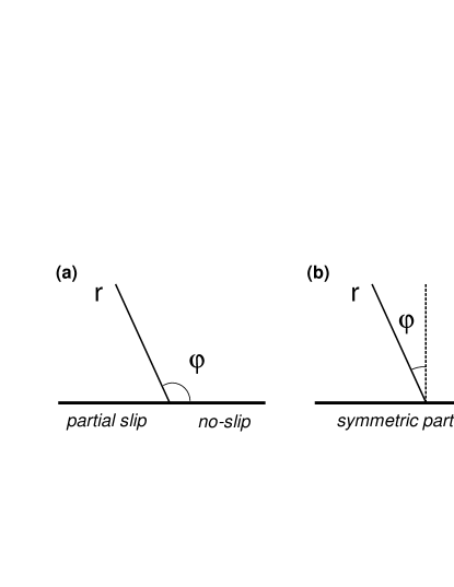
Figure 6: Polar coordinate systems for (a) trapezoidal and (b) triangular profiles of the local slip length. For a mathematical convenience the two coordinates differ in the choice of the origin of the angular variable $\varphi$.

We begin by studying the trapezoidal slip profile. For the trapezoid, the origin of coordinates is at $(y_{e},z_{e})=(\phi_{1}/2,0)$, with $y=\phi_{1}/2+r\cos\varphi$ and $z=r\sin\varphi$, $0\leq\varphi\leq\pi$, so that the n o-slip and the slip regions correspond to $\varphi=0\$and $\varphi=\pi$. The slip condition (13) becomes

$$r\ll 1,\ \varphi=\pi:\quad u-\xi r\partial_{z}u=\xi r,$$ (34)

where $\xi$ is defined as

$$\xi=\frac{2b_{2}}{L\left(1-\phi_{1}-\phi_{2}\right)},$$ (35)

and can vary from $0$ to $\infty$, depending on the local slip, $b_{2}/L$, and on the value of $\phi_{1}+\phi_{2}$. In the case of stripes, one has $\phi_{1}+\phi_{2}=1$, resulting in $\xi\to\infty$ at finite $b_{2}/L$.

The solution of Eq. (12) that satisfies the no-slip boundary condition at $\varphi=0$ is given by

$$u=cr^{\lambda^{\parallel}}\sin\left(\lambda^{\parallel}\varphi\right),$$ (36)

and the components of the velocity gradient are

$$\partial_{z}u = c\lambda^{\parallel}r^{\lambda^{\parallel}-1}\cos\left[\varphi\left(1-\lambda^{\parallel}\right)\right],$$ (37)

$$\partial_{y}u = -c\lambda^{\parallel}r^{\lambda^{\parallel}-1}\sin\left[\varphi\left(1-\lambda^{\parallel}\right)\right].$$ (38)

The velocity at the edge is finite provided $\lambda^{\parallel}>0,$ but its gradient becomes singular when $\lambda^{\parallel}<1$. In this case the two terms in the left-hand side of Eq. (34) are of the same order, $r^{\lambda^{\parallel}}$, but the right-hand side is smaller and can be neglected, since $r\ll r^{\lambda^{\parallel}}$ as $\lambda^{\parallel}<1$. As a result Eq. (34) can be rewritten, taking into account (36-38) as

$$\sin\left(\lambda^{\parallel}\pi\right)-\xi\lambda^{\parallel}\cos\left[\left(1-\lambda^{\parallel}\right)\pi\right]=0,$$

or equivalently as,

$$(\lambda^{\parallel})^{-1}\tan\left(\lambda^{\parallel}\pi\right)=-\xi.$$ (39)

The theoretical prediction of Eq. (39) for the behavior of $\lambda^{\parallel}$ as a function of $\xi$ is shown in Fig. 7 (solid curve). Note that $\lambda^{\parallel}$ decays monotonically from $\lambda^{\parallel}(\xi\rightarrow 0)\rightarrow 1$ down to $\lambda^{\parallel}(\xi\rightarrow\infty)\rightarrow 1/2$. In other words, for any finite $\xi$, we have $\lambda^{\parallel}<1,$ and the shear stress becomes singular. As shown in Fig. 7 these theoretical predictions are in excellent quantitative agreement with the simulation results, where we have measured the slip velocity along the surface and then obtained $\lambda^{\parallel}$ by using Eq. (36). Altogether the theoretical and numerical results confirm that the singular is weaker for trapezoidal profiles than for stripes, such that the viscous dissipation is smaller. This explains qualitatively the results presented in Fig. 5, where the slip length deviates more strongly from the area-averaged slip length on striped than on trapezoidal textures.

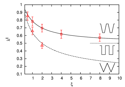
Figure 7: Exponents $\lambda^{\parallel}=1/2$ (see text for definition) for the trapezoid [Eq. (36), solid line] and triangle slip profiles [Eq.  (40), dashed line] As a reference, the exponent $\lambda^{\parallel}=1/2$ for striped surfaces is also shown as dotted line. Symbols are simulation data.

In the theoretical analysis of the triangular slip profile ($\phi_{1}=0$) it is convenient to shift the origin of the angular variable $\phi$ compared to the trapezoidal case (see Fig. 6), so that $z=r\cos\varphi,$ $y=r\sin\varphi,$ $\left|\varphi\right|\leq\pi/2.$

The even solution of the Laplace equation (12) is

$$u=cr^{\lambda^{\parallel}}\cos\left(\lambda^{\parallel}\varphi\right),$$ (40)

and the components of the velocity gradient are then

$$\partial_{z}u = c\lambda^{\parallel}r^{\lambda^{\parallel}-1}\cos\left[\varphi\left(1+\lambda^{\parallel}\right)\right],$$ (41)

$$\partial_{y}u = -c\lambda^{\parallel}r^{\lambda^{\parallel}-1}\sin\left[\varphi\left(1+\lambda^{\parallel}\right)\right].$$ (42)

The slip condition (13) at $\varphi=\pm\pi/2$ can be rewritten as

$$cr^{\lambda^{\parallel}}\left\{\cos\left(\lambda^{\parallel}\frac{\pi}{2}\right)-\xi\lambda^{\parallel}\cos\left[\left(1+\lambda^{\parallel}\right)\frac{\pi}{2}\right]\right\}=\xi r,$$ (43)

with

$$\xi=2b_{2}/L.$$ (44)

Applying the condition $\lambda^{\parallel}<1$, we can neglect the right-hand side to obtain

$$\lambda^{\parallel}\tan\left(\lambda^{\parallel}\frac{\pi}{2}\right)=\xi^{-1}.$$ (45)

The numerical solution of this equation is included in Fig. 7 (dashed curve), and supported by simulation data. We see that $\lambda^{\parallel}$ again decays monotonically from $\lambda^{\parallel}(\xi\rightarrow 0)=1$, but at large $\xi$ the solution of Eq. (45) is

$$\lambda^{\parallel}=\left(\frac{2}{\pi\xi}\right)^{1/2}\ll 1,$$

i.e., different from expected for a trapezoidal profile, where $\lambda^{\parallel}$ would tend to 0.5. This implies that for given $\xi$, the triangular slip profile always gives a stronger singularity compared to a trapezoid slip profile. At small $\xi$, the singularity is weaker than for a striped surface.

A striking conclusion from our analysis is that non-smooth surface textures with continuous local slip can generate stronger singularities in flow and shear stress than surfaces with a discontinuous, piece-wise constant slip length profile. Indeed, we have $\lambda^{\parallel}>1/2$ for $\xi>2$ (or $b_{2}>L$), i.e., the singularity for a triangular texture becomes stronger than for stripes and should significantly reduce the longitudinal effective slip. This is likely a reason why the effective slip in Fig. 4(b) grows only weakly at very large $b_{2}/L$. Coming back to Fig. 5, we remark that the results for triangular profile there correspond to $\xi=0.5$ and $\lambda^{\parallel}\simeq 0.77$, i.e., the singularity is weaker in this case than for stripes with $\lambda^{\parallel}=0.5$. The singularities for trapezoidal profiles may be even weaker: The exponents vary from $\lambda^{\parallel}\simeq 0.87$ to $\lambda^{\parallel}\simeq 0.5$. Note however that since the no-slip area remains the key factor determining the effective slip, $b_{\rm eff}^{\parallel}$ always decreases with $\phi_{1}$.

To calculate the exponents $\lambda^{\perp}$ for a transverse configuration, one can use the relation between the velocity fields in eigendirections Asmolov and Vinogradova (2012):

$$v=\frac{1}{2}\left(u_{d}+z\frac{\partial u_{d}}{\partial z}\right),\quad w=-\frac{z}{2}\frac{\partial u_{d}}{\partial y},$$ (46)

$$p=-\frac{\partial u_{d}}{\partial y},$$ (47)

where $u_{d}\left(y,z\right)=u\left[y,z,2b\left(y\right)/L\right]$ is the velocity field for the longitudinal pattern with a twice larger local slip length. It follows from Eqs. (46) and (47), that the velocity gradients and the pressure in the transverse configuration for both trapezoidal and triangular textures have stronger singularities at the edges of slipping regions than those for the longitudinal configuration:

$$\frac{\partial v}{\partial z},\ \frac{\partial w}{\partial z},\ p\sim r^{\lambda^{\perp}-1},$$

where $\lambda^{\perp}=\lambda^{\parallel}\left(2\xi\right)<\lambda^{\parallel}\left(\xi\right)$. This leads to larger viscous dissipation. As a result the anisotropy of the slip-length tensor is finite even at small $b_{2}/L$ and is approximately the same for triangular, trapezoidal and stripe profiles ( see Fig. 5). For example, the eigenvalues shown there for a triangular texture correspond to $\lambda^{\parallel}\simeq 0.77$ and $\lambda^{\perp}\simeq 0.64$. Therefore, in the transverse configuration even for a shallow triangular texture, $b_{2}>L/2$, the singularity becomes stronger than for stripes ($\lambda^{\perp}>1/2)$.

VI Optimization of the effective slip

Based on the results obtained in the previous sections, we now discuss how to optimize the effective slippage, and what maximum slip lengths may actually be expected, taking into account the actual limitation in surface engineering.

Very large effective slip lengths were recently found for sinusoidal profiles $b(y)$ with a no-slip point Asmolov et al. (2013b). If we request that the local slip pattern includes a no-slip area, we also find here that the largest values of $b_{\rm eff}$ are obtained for triangular profiles, where the no-slip area reduces to just one point. However, real textures always have finite contact area with liquid. The effective slip length of a trapezoidal texture with large $b_{2}/L$ is close to that of stripes [see Fig. 4(a)]. In this final section, we therefore focus on the case of a trapezoidal profile with small $\phi_{1}$, where both $b_{2}/L$ and the slope of the inclined regions is large. Such a texture should lead to large $b_{\mathrm{eff}}$. To find one-dimensional textures which optimize the effective forward slip we consider profiles of the following form

$$\frac{b(y)}{L}=\begin{cases}0,&|t|\leq\frac{\phi_{1}}{2}\\ \frac{2|t|-\phi_{1}}{9\phi_{1}^{2}},&\frac{\phi_{1}}{2}<|t|\leq 5\phi_{1}\\ \phi_{1}^{-1},&5\phi_{1}<|t|\leq\frac{1}{2},\ \phi_{1}<0.1\end{cases}$$ (48)

The bottom base of the trapezoid for such textures is wide, $10\phi_{1}$, [see Fig. 8(a)]. For comparison, we also consider stripes with the same maximal local slip length, $b_{2}/L=\phi_{1}^{-1}$:

$$\frac{b(y)}{L}=\begin{cases}0,&|t|\leq\frac{\phi_{1}}{2}\\ \phi_{1}^{-1},&\frac{\phi_{1}}{2}<|t|\leq\frac{1}{2}\end{cases}$$ (49)

Both profiles are characterized by only one parameter $\phi_{1}$.

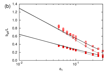
Figure 8: (a) Profiles of local slip length resulting in the same $b_{\rm eff}^{\parallel}$, (b) Effective slip lengths for stripe (solid lines and square symbols) and trapezoidal (dotted lines and circular symbols) local slip profiles. The top and bottom lines correspond to $b_{\rm eff}^{\parallel}$ and $b_{\rm eff}^{\perp}$, respectively.

The simulation and numerical results for $b_{\rm eff}^{\parallel}$ and $b_{\rm eff}^{\perp}$ are shown in Fig. 8(b). The effective slip lengths for the trapezoid and stripe profiles are nearly equal for $\phi_{1}<0.1$. For example, $b_{\rm eff}^{\parallel}$ for the stripe profile with $\phi_{1}=0.05$ is only slightly larger than the corresponding value for the trapezoid profile with the same $\phi_{1}$ and wide bottom base [see Fig. 8(a)]. Note that such narrow trapezoids with wide bottom base allowed researchers to achieve a very large effective slip in recent experiments Choi et al. (2006). The same value of $b_{\rm eff}^{\parallel}$ can be achieved with a triangular profile with $b_{\mathrm{max}}/L=4$. Thus the effect of the inclined regions is relatively small for large slopes, and the main contribution to the effective slip length stems from the no-slip region and the singularity of the shear stress.

VII Concluding Remarks

In conclusion, we have presented simulation and numerical results and some asymptotic law analysis that allowed us to assess the frictional properties of superhydrophobic surfaces as a function of the texture geometric parameters. We have focused on one-dimensional superhydrophobic surfaces with trapezoidal grooves and systematically investigated the effect of several parameters, such as the maximum local slip and the heterogeneity factor. The slip properties on a trapezoidal surface were compared with two limiting cases: striped and triangular slip length profiles. Our simulation and numerical results suggested that the effective slip length is mainly determined by (i) the area fraction of the no-slip region and (ii) the singularity of the shear stress at the no-slip edge. The first factor is obvious; a smaller fraction of no-slip area results in less friction of the surface, which in turn leads to large slip length. The second effect is less intuitive, especially for a continuous slip profile. Here we demonstrated that the singularity develops for the trapezoidal and triangular local slip profiles, and in the latter case can be even stronger than for discontinuous slip of striped textures. The singularity is stronger for a transverse configuration in comparison to a longitudinal configuration, and as a result, it always contributes to the flow anisotropy. Our results can guide the design of superhydrophobic surfaces for micro/nanofluidics.