Model Reduction Near Periodic Orbits
of Hybrid Dynamical Systems

Abstract

We show that, near periodic orbits, a class of hybrid models can be reduced to or approximated by smooth continuous–time dynamical systems. Specifically, near an exponentially stable periodic orbit undergoing isolated transitions in a hybrid dynamical system, nearby executions generically contract superexponentially to a constant–dimensional subsystem. Under a non–degeneracy condition on the rank deficiency of the associated Poincaré map, the contraction occurs in finite time regardless of the stability properties of the orbit. Hybrid transitions may be removed from the resulting subsystem via a topological quotient that admits a smooth structure to yield an equivalent smooth dynamical system. We demonstrate reduction of a high–dimensional underactuated mechanical model for terrestrial locomotion, assess structural stability of deadbeat controllers for rhythmic locomotion and manipulation, and derive a normal form for the stability basin of a hybrid oscillator. These applications illustrate the utility of our theoretical results for synthesis and analysis of feedback control laws for rhythmic hybrid behavior.

I Introduction

Rhythmic phenomena are pervasive, appearing in physical situations as diverse as legged locomotion [1], dexterous manipulation [2], gene regulation [3], and electrical power generation [4]. The most natural dynamical models for these systems are piecewise–defined or discontinuous owing to intermittent changes in the mechanical contact state of a locomotor or manipulator, or to rapid switches in protein synthesis or constraint activation in a gene or power network. Such hybrid systems generally exhibit dynamical behaviors that are distinct from those of smooth systems [5]. Restricting our attention to the dynamics near periodic orbits in hybrid dynamical systems, we demonstrate that a class of hybrid models for rhythmic phenomena reduce to classical (smooth) dynamical systems.

Although the results of this paper do not depend on the phenomenology of the physical system under investigation, a principal application domain for this work is terrestrial locomotion. Numerous architectures have been proposed to explain how animals control their limbs; for steady–state locomotion, most posit a principle of coordination, synergy, symmetry or synchronization, and there is a surfeit of neurophysiological data to support these hypotheses [6, 7, 8, 9, 10]. Taken together, the empirical evidence suggests that the large number of degrees–of–freedom (DOF) available to a locomotor can collapse during regular motion to a low–dimensional dynamical attractor (a template) embedded within a higher–dimensional model (an anchor) that respects the locomotor’s physiology [1, 11]. We provide a mathematical framework to model this empirically observed dimensionality reduction in the deterministic setting.

A stable hybrid periodic orbit provides a natural abstraction for the dynamics of steady–state legged locomotion. This widely–adopted approach has generated models of bipedal [12, 13, 14, 15] and multi–legged [16, 17, 18] locomotion as well as control–theoretic techniques for composition [19], coordination [20], and stabilization [21, 22, 23]. In certain cases, it has been possible to embed a low–dimensional abstraction in a higher–dimensional model [24, 25]. Applying these techniques to establish existence of a reduced–order subsystem imposes stringent assumptions on the dynamics of locomotion that are difficult to verify for any particular locomotor. In contrast, the results of this paper imply that hybrid dynamical systems generically exhibit dimension reduction near periodic orbits solely due to the interaction of the discrete–time switching dynamics with the continuous–time flow.

Under the hypothesis that iterates of the Poincaré map  associated with a periodic orbit in a hybrid dynamical system are eventually constant rank, we construct a constant–dimensional invariant subsystem that attracts all nearby trajectories in finite time regardless of the stability properties of the orbit; this appears as Theorem 1 of Section III-C, below. Assuming instead that the periodic orbit under investigation is exponentially stable, we show in Theorem 2 of Section III-D that trajectories generically contract superexponentially to a subsystem whose dimension is determined by rank properties of the linearized Poincaré map  at a single point. The resulting subsystems possess a special structure that we exploit in Theorem 3 to construct a topological quotient that removes the hybrid transitions and admits the structure of a smooth manifold, yielding an equivalent smooth dynamical system.

In Section IV we apply these results to reduce the complexity of hybrid models for mechanical systems and analyze rhythmic hybrid control systems. The example in Section IV-A demonstrates that reduction can occur spontaneously in mechanical systems undergoing plastic impacts. In Section IV-B we prove that a family of $(3+2n)$–DOF multi–leg models provably reduce to a common 3–DOF mechanical system independent of the number of limbs, $n\in\mathbb{N}$; this demonstrates model reduction in the mechanical component of the class of neuromechanical models considered in [1, 18]. As further applications, we assess structural stability of deadbeat controllers for rhythmic locomotion and manipulation in Section IV-C and derive a normal form for the stability basin of a hybrid oscillator in Section IV-D.

II Preliminaries

We assume familiarity with differential topology and geometry [26, 27], and summarize notation and terminology in this section for completeness.

If $(X,\left\|\cdot\right\|)$ is a Banach space, we let $B_{\delta}(x)\subset X$ denote the open ball of radius $\delta>0$ centered at $x\in X$; For $X=\mathbb{R}^{n}$, we may emphasize the dimension $n$ by writing $B^{n}_{\delta}(0)\subset\mathbb{R}^{n}$ for the open $\delta$–ball. A subset of a topological space is precompact if it is open and its closure is compact. A neighborhood of a point $x\in X$ in a topological space $X$ is a connected open subset $U\subset X$ containing $x$. The disjoint union of a collection of sets $\left\{S_{j}\right\}_{j\in J}$ is denoted $\coprod_{j\in J}S_{j}=\bigcup_{j\in J}S_{j}\times\left\{j\right\}$, a set we endow with the natural piecewise–defined topology. If ${\sim}\subset D\times D$ is an equivalence relation on the topological space $D$, then we let $D/{\sim}$ denote the corresponding set of equivalence classes. There is a natural quotient projection $\pi:D\rightarrow D/{\sim}$ sending $x\in D$ to its equivalence class $\left[x\right]\in D/{\sim}$, and we endow $D/{\sim}$ with the (unique) finest topology making $\pi$ continuous [27, Appendix A]. Any map $R:G\rightarrow D$ defined over a subset $G\subset D$ determines an equivalence relation ${\sim}=\left\{(x,y)\in D\times D:x\in R^{-1}(y),\ y\in R^{-1}(x),\ \text{or}\ x=y\right\}$. To be explicit that the equivalence relation is determined by $R$ we denote the quotient space as

$$D/{\sim}=\frac{D}{G\overset{R}{\sim}R(G)}.$$

A $C^{r}$ $n$–dimensional manifold $M$ with boundary $\partial M$ is an $n$–dimensional topological manifold covered by an atlas of $C^{r}$ coordinate charts $\left\{(U_{\alpha},\varphi_{\alpha})\right\}_{\alpha\in\mathscr{A}}$ where $U_{\alpha}\subset M$ is open, $\varphi_{\alpha}:U_{\alpha}\rightarrow H^{n}$ is a homeomorphism, and $H^{n}=\left\{(y_{1},\dots,y_{n})\in\mathbb{R}^{n}:y_{n}\geq 0\right\}$ is the upper half–space; we write $\dim M=n$. The charts are $C^{r}$ in the sense that $\varphi_{\alpha}\circ\varphi_{\beta}^{-1}$ is a $C^{r}$ diffeomorphism over $\varphi_{\beta}(U_{\alpha}\cap U_{\beta})$ for all pairs $\alpha,\beta\in\mathscr{A}$ for which $U_{\alpha}\cap U_{\beta}\neq\emptyset$; if $r=\infty$ we say $M$ is smooth. The boundary $\partial M\subset M$ contains those points that are mapped to the plane $\left\{(y_{1},\dots,y_{n})\in\mathbb{R}^{n}:y_{n}=0\right\}$ in some chart. A map $P:M\rightarrow N$ is $C^{r}$ if $M$ and $N$ are $C^{r}$ manifolds and for every $x\in M$ there is a pair of charts $(U,\varphi),(V,\psi)$ with $x\in U\subset M$ and $P(x)\in V\subset N$ such that the coordinate representation $\widetilde{P}=\psi\circ P\circ\varphi^{-1}$ is a $C^{r}$ map between subsets of $H^{n}$. We let $C^{r}(M,N)$ denote the normed vector space of $C^{r}$ maps between $M$ and $N$ endowed with the uniform $C^{r}$ norm [26, Chapter 2].

Each $x\in M$ has an associated tangent space $T_{x}M$, and the disjoint union of the tangent spaces is the tangent bundle $TM=\coprod_{x\in M}T_{x}M$. Note that any element in $TM$ may be regarded as a pair $(x,\delta)$ where $x\in M$ and $\delta\in T_{x}M$, and $TM$ is naturally a smooth $2n$–dimensional manifold. We let $\mathscr{T}(M)$ denote the set of smooth vector fields on $M$, i.e. smooth maps $F:M\rightarrow TM$ for which $F(x)=(x,\delta)$ for some $\delta\in T_{x}M$ and all $x\in M$. It is a fundamental result that any $F\in\mathscr{T}(M)$ determines an ordinary differential equation in every chart on the manifold that may be solved globally to obtain a maximal flow $\phi:\mathscr{F}\rightarrow M$ where $\mathscr{F}\subset\mathbb{R}\times M$ is the maximal flow domain [27, Theorem 17.8].

If $P:M\rightarrow N$ is a smooth map between smooth manifolds, then at each $x\in M$ there is an associated linear map $DP(x):T_{x}M\rightarrow T_{P(x)}N$ called the pushforward. Globally, the pushforward is a smooth map $DP:TM\rightarrow TN$; in coordinates, it is the familiar Jacobian matrix. If $M=X\times Y$ is a product manifold, the pushforward naturally decomposes as $DP=\left(D_{x}P,\,D_{y}P\right)$ corresponding to derivatives taken with respect to $X$ and $Y$, respectively. The rank of a smooth map $P:M\rightarrow N$ at a point $x\in M$ is $\operatorname{rank}DP(x)$. If $\operatorname{rank}DP(x)=r$ for all $x\in M$, we simply write $\operatorname{rank}DP\equiv r$. If $P$ is furthermore a homeomorphism onto its image, then $P$ is a smooth embedding, and the image $P(M)$ is a smooth embedded submanifold. In this case the difference $\dim N-\dim P(M)$ is called the codimension of $P(M)$, and any smooth vector field $F\in\mathscr{T}(M)$ may be pushed forward to a unique smooth vector field $DP(F)\in\mathscr{T}(P(M))$. A vector field $F\in\mathscr{T}(M)$ is inward–pointing at $x\in\partial M$ if for any coordinate chart $(U,\varphi)$ with $x\in U$ the $n$–th coordinate of $D\varphi(F)$ is positive and outward–pointing if it is negative.

III Hybrid Dynamical Systems

We describe a class of hybrid systems useful for modeling physical phenomena in Section III-A, then restrict our attention to the behavior of such systems near periodic orbits in Section III-B. It was shown in [28] that the Poincaré map associated with a periodic orbit of a hybrid system is generally not full rank; we explore the geometric consequences of this rank loss. Under a non–degeneracy condition on this rank loss we demonstrate in Section III-C that the hybrid system possesses an invariant hybrid subsystem to which all nearby trajectories contract in finite time regardless of the stability properties of the orbit. In Section III-D we show that the invariance and contraction of the subsystem hold approximately for any exponentially stable hybrid periodic orbit. Using tools from differential topology, we remove hybrid transitions from the resulting reduced–order subsystems in Section III-E to yield a continuous–time dynamical system that governs the behavior of the hybrid system near its periodic orbit.

III-A Hybrid Differential Geometry

For our purposes, it is expedient to define hybrid dynamical systems over a finite disjoint union $M=\coprod_{j\in J}M_{j}$ where $M_{j}$ is a connected manifold with boundary for each $j\in J$; we endow $M$ with the natural (piecewise–defined) topology and smooth structure. We refer to such spaces as smooth hybrid manifolds. Note that the dimensions of the constituent manifolds are not required to be equal. Several differential–geometric constructions naturally generalize to such spaces; we prepend the modifier ‘hybrid’ to make it clear when this generalization is invoked. For instance, the hybrid tangent bundle $TM$ is the disjoint union of the tangent bundles $TM_{j}$, and the hybrid boundary $\partial M$ is the disjoint union of the boundaries $\partial M_{j}$.

Let $M=\coprod_{j\in J}M_{j}$ and $N=\coprod_{\ell\in L}N_{\ell}$ be two hybrid manifolds. Note that if a map $R:M\rightarrow N$ is continuous, then for each $j\in J$ there exists $\ell\in L$ such that $R(M_{j})\subset N_{\ell}$ and hence $R|_{M_{j}}:M_{j}\rightarrow N_{\ell}$. Using this observation, there is a natural definition of differentiability for continuous maps between hybrid manifolds. Namely, a map $R:M\rightarrow N$ is called smooth if $R$ is continuous and $R|_{M_{j}}:M_{j}\rightarrow N$ is smooth for each $j\in J$. In this case the pushforward $DR:TM\rightarrow TN$ is the smooth map defined piecewise as $DR|_{TM_{j}}=D(R|_{M_{j}})$ for each $j\in J$. A smooth map $F:M\rightarrow TM$ is called a vector field if for all $x\in M$ there exists $v\in T_{x}M$ such that $F(x)=(x,v)$.

With these preliminaries established, we define the class of hybrid systems considered in this paper. This is a specialization of hybrid automata [5] that emphasizes the differential–geometric character of hybrid phenomena.

Definition 1.

A hybrid dynamical system is specified by a tuple $H=(D,F,G,R)$ where:

• $=\coprod_{j\in J}D_{j}$ is a smooth hybrid manifold;

• $:D\rightarrow TD$ is a smooth vector field;

• $\subset\partial D$ is an open subset of $\partial D$;

• $:G\rightarrow D$ is a smooth map.

As in [5], we call $R$ the reset map and $G$ the guard. When we wish to be explicit about the order of smoothness, we will say $H$ is $C^{r}$ if $D$, $F$, and $R$ are $C^{r}$ as a manifold, vector field, and map, respectively, for some $r\in\mathbb{N}$.

Roughly speaking, an execution of a hybrid dynamical system is determined from an initial condition in $D$ by following the continuous–time dynamics determined by the vector field $F$ until the trajectory reaches the guard $G$, at which point the reset map $R$ is applied to obtain a new initial condition.

Definition 2.

An execution of a hybrid dynamical system $H=(D,F,G,R)$ is a right–continuous function $x:T\rightarrow D$ over an interval $T\subset\mathbb{R}$ such that:

1. if $x$ is continuous at $t\in T$, then $x$ is differentiable at $t$ and $\frac{d\,}{dt}x(t)=F(x(t))$;

2. if $x$ is discontinuous at $t\in T$, then the limit $x(t^{-})=\displaystyle\lim_{s\rightarrow t^{-}}x(s)$ exists, $x(t^{-})\in G$, and $\displaystyle R(x(t^{-}))=x(t)$.

If $F$ is tangent to $G$ at $x\in G$, there is a possible ambiguity in determining a trajectory from $x$ since one may either follow the flow of $F$ on $D$ or apply the reset map to obtain a new initial condition $y=R(x)$.

Assumption 1.

$F$ is outward–pointing on $G$.

Remark 1.

The use of time–invariant vector fields and reset maps in Definition 1 is without loss of generality in the following sense. Suppose $D$ is a hybrid manifold, $G\subset\partial D$ is open, and $F:\mathbb{R}\times D\rightarrow TD$, $R:\mathbb{R}\times G\rightarrow D$ define a time–varying vector field and reset map, respectively. Define

$${\normalsize{{{\widehat{D}}}}}=\mathbb{R}\times D,\ {\normalsize{{{\widehat{G}}}}}=\mathbb{R}\times G,$$

and let ${\normalsize{{{\widehat{F}}}}}:{\normalsize{{{\widehat{D}}}}}\rightarrow T{\normalsize{{{\widehat{D}}}}}$, ${\normalsize{{{\widehat{R}}}}}:{\normalsize{{{\widehat{G}}}}}\rightarrow{\normalsize{{{\widehat{D}}}}}$ be defined in the obvious way. Then ${\normalsize{{{\widehat{H}}}}}=({\normalsize{{{\widehat{D}}}}},{\normalsize{{{\widehat{F}}}}},{\normalsize{{{\widehat{G}}}}},{\normalsize{{{\widehat{R}}}}})$ is a hybrid dynamical system in the form of Definition 1.

III-B Hybrid Periodic Orbits and Hybrid Poincaré Maps

In this paper, we are principally concerned with periodic executions of hybrid dynamical systems, which are nonequilibrium trajectories that intersect themselves.

Definition 3.

An execution $\gamma:T\rightarrow D$ is periodic if there exists $s\in T$, $\tau>0$ such that $s+\tau\in T$ and

$$\gamma(s)=\gamma(s+\tau).$$ (1)

If there is no smaller positive number $\tau$ such that (1) holds, then $\tau$ is called the period of $\gamma$, and we will say $\gamma$ is a $\tau$–periodic orbit.

Remark 2.

The domain $T$ of a periodic orbit may be taken to be the entire real line, $T=\mathbb{R}$, without loss of generality. In the sequel we conflate the execution $\gamma:\mathbb{R}\rightarrow D$ with its image $\gamma(\mathbb{R})\subset D$.

Motivated by the applications in Section IV, we restrict our attention to periodic orbits undergoing isolated discrete transitions, i.e. a finite number of discrete transitions that occur at distinct time instants.

Assumption 2.

$\gamma$ undergoes isolated discrete transitions.

In addition to excluding Zeno periodic orbits [29] from our analysis, this assumption enables us to construct Poincaré maps (see [30, 31] for the classical case) associated with $\gamma$. A Poincaré map $P:U\rightarrow\Sigma$ is defined over an open subset $U\subset\Sigma$ of an embedded codimension–1 submanifold $\Sigma\subset D$ that intersects the periodic orbit at one point $\left\{\xi\right\}=\gamma\cap\Sigma$ by tracing an execution from $x\in U$ forward in time until it intersects $\Sigma$ at $P(x)$. The submanifold $\Sigma$ is referred to as a Poincaré section. It is known that this procedure yields a map that is well–defined and smooth near the fixed point $\xi=P(\xi)$ [32, 13, 28, 33]. Unlike the classical case, Poincaré maps in hybrid systems need not be full rank.

A straightforward application of Sylvester’s inequality [34, Appendix A.5.3] shows that the rank of the Poincaré map is bounded above by the minimum dimension of all hybrid domains. More precise bounds are pursued elsewhere [28], but the following Proposition will suffice for the Applications in Section IV.

Proposition 1.

If $P:U\rightarrow\Sigma$ is a Poincaré map associated with a periodic orbit $\gamma$, then $\forall x\in U:\operatorname{rank}DP(x)\leq\min_{j\in J}\dim D_{j}-1$.

It is a standard result for continuous–time dynamical systems that the eigenvalues of the linearization of the Poincaré map at its fixed point—commonly called Floquet multipliers—do not depend on the choice of Poincaré section [31, Section 1.5]. This generalizes to the hybrid setting in the sense that there exist similarity transformations relating the non–nilpotent portion of the Jordan forms for linearizations of Poincaré maps defined over different sections. Note that, since Proposition 1 implies that zero eigenvalues will generally have different algebraic multiplicity for linearized Poincaré maps obtained from sections located in hybrid domains with different dimensions, we do not expect the nilpotent Jordan blocks for these linear maps to bear any relation to one another. These observations are summarized in the following Lemma.

Lemma 1.

If $P:U\rightarrow\Sigma$, ${\normalsize{{{\widehat{P}}}}}:{\normalsize{{{\widehat{U}}}}}\rightarrow{\normalsize{{{\widehat{\Sigma}}}}}$ are Poincaré maps associated with a periodic orbit $\gamma$ with fixed points $P(\xi)=\xi$, ${\normalsize{{{\widehat{P}}}}}({\normalsize{{{\widehat{\xi}}}}})={\normalsize{{{\widehat{\xi}}}}}$, then $\operatorname{spec}DP(\xi)\setminus\left\{0\right\}=\operatorname{spec}D{\normalsize{{{\widehat{P}}}}}({\normalsize{{{\widehat{\xi}}}}})\setminus\left\{0\right\}$. Moreover, with

$$J=\left(\begin{array}[]{cc}A&0\\ 0&N\end{array}\right),\ {\normalsize{{{\widehat{J}}}}}=\left(\begin{array}[]{cc}{\normalsize{{{\widehat{A}}}}}&0\\ 0&{\normalsize{{{\widehat{N}}}}}\end{array}\right)$$

denoting the Jordan canonical forms of $DP(\xi)$ and $D{\normalsize{{{\widehat{P}}}}}({\normalsize{{{\widehat{\xi}}}}})$, where $0\not\in\operatorname{spec}A\cup\operatorname{spec}{\normalsize{{{\widehat{A}}}}}$ and $N$, ${\normalsize{{{\widehat{N}}}}}$ are nilpotent, we conclude that $A$ is similar to ${\normalsize{{{\widehat{A}}}}}$.

Proof.

The periodic orbit undergoes a finite number of transitions $k\in\mathbb{N}$, so we may index the corresponding sequence of domains as $D_{1},\dots,D_{k}$. Without loss of generality, assume the $D_{j}$’s are distinct and let $\left\{{\normalsize{{{\xi_{j}}}}}\right\}=\gamma\cap G\cap\partial D_{j}$ be the exit point of $\gamma$ in $D_{j}$. We wish to construct the Poincaré map $P_{j}$ associated with the periodic orbit over a neighborhood of $\xi_{j}$ in $G$. For $j\in\left\{1,\dots,k\right\}$ let:

1. $:\mathscr{F}_{j}\rightarrow D_{j}$ be the maximal flow of $F|_{D_{j}}$ on $D_{j}$;

2. $\subset D_{j}$ be a neighborhood of $R(\xi_{j-1})$ over which Lemma 2 from Appendix A-A1 may be applied between $R(\xi_{j-1})\in D_{j}$ and $G\cap\partial D_{j}$ to obtain a time–to–impact map $\sigma_{j}:U_{j}\rightarrow\mathbb{R}$;

3. $\subset G\cap\partial D_{j}$ be defined as $G_{j}=R^{-1}(U_{j+1})$;

4. $:G_{j}\rightarrow G_{j+1}$ be defined by $\rho_{j}(x)=\phi_{j+1}\left(\sigma_{j+1}\circ{R(x)},R(x)\right)$.

The Poincaré map defined over $G_{j}$ is obtained formally by iterating the $\rho$’s around the cycle:

$$P_{j}=\rho_{j-1}\circ\cdots\circ\rho_{1}\circ\rho_{k}\circ\cdots\circ\rho_{j}.$$ (2)

The neighborhood $\Sigma_{j}\subset G_{j}$ of $\xi_{j}$ over which this map is well–defined is determined by pulling $G_{j}$ backward around the cycle,

$$\Sigma_{j}=\left(\rho_{j}^{-1}\circ\cdots\circ\rho_{k}^{-1}\circ\rho_{1}^{-1}\circ\cdots\circ\rho_{j-1}^{-1}\right)(G_{j}),$$

and similarly for any iterate of $P_{j}$. Note that $P_{j}(\xi_{j})=\xi_{j}$ is a fixed point of $P_{j}$ by construction. Without loss of generality we assume $\Sigma,{\normalsize{{{\widehat{\Sigma}}}}}\subset G$ so that $P=P_{j}$ and ${\normalsize{{{\widehat{P}}}}}=P_{i}$ for some $i,j\in\left\{1,\dots,k\right\}$. Refer to Fig. 1 for an illustration.

Figure 1: Illustration of constructions used in proofs of Lemma 1, Theorem 1, and Theorem 2. For each $j\in J$, the periodic orbit $\gamma$ intersects the guard in domain $D_{j}$ at $\left\{\xi_{j}\right\}=\gamma\cap G\cap\partial D_{j}$. A neighborhood $U_{j}\subset D_{j}$ of $R(\xi_{j-1})$ flows via the vector field $F|_{D_{j}}$ to reach a neighborhood $G_{j}\subset G\cap\partial D_{j}$ of $\xi_{j}$ obtained via $G_{j}=R^{-1}(U_{j+1})$. The neighborhood $\Sigma_{j}\subset G_{j}$ of $\xi_{j}$ is chosen sufficiently small to ensure executions initialized in $\Sigma_{j}$ return to $G_{j}$ via the Poincaré map $P_{j}:\Sigma_{j}\rightarrow G_{j}$ after one cycle.

We proceed by showing that, given a chain of generalized eigenvectors associated with a non–zero eigenvalue of $DP_{j}(\xi_{j})$ for some $j\in\left\{1,\dots,k\right\}$, we can construct a chain of generalized eigenvectors associated with $DP_{i}(\xi_{i})$ with the same eigenvalue for each $i\in\left\{1,\dots,k\right\}$. Fix $j\in\left\{1,\dots,k\right\}$ and $\lambda\in\operatorname{spec}DP_{j}(\xi_{j})$ with $\lambda\neq 0$. Suppose $\left\{x_{j}^{\ell}\right\}_{\ell=1}^{m}$ is a chain of generalized eigenvectors associated with $\lambda$, i.e. $DP_{j}(\xi_{j})x_{j}^{m}=\lambda x_{j}^{m}$ and for all $\ell\in\left\{1,\dots,m-1\right\}$:

$$x_{j}^{\ell}=(DP_{j}(\xi_{j})-\lambda I)x_{j}^{\ell+1}.$$ (3)

For all $\ell\in\left\{1,\dots,m\right\}$, define $x_{j+1}^{\ell}=D\rho_{j}(\xi_{j})x_{j}^{\ell}$ and note $D\rho_{j}(\xi_{j})DP_{j}(\xi_{j})=DP_{j+1}(\xi_{j+1})D\rho_{j}(\xi_{j})$ by (2). Combining this observation with (3) yields

$$DP_{j+1}(\xi_{j+1})x_{j+1}^{m} =DP_{j+1}(\xi_{j+1})D\rho_{j}(\xi_{j})x_{j}^{m}$$

$$=D\rho_{j}(\xi_{j})DP_{j}(\xi_{j})x_{j}^{m}$$

$$=\lambda D\rho_{j}(\xi_{j})x_{j}^{m}=\lambda x_{j+1}^{m},$$

so that $\lambda\in\operatorname{spec}DP_{j+1}(\xi_{j+1})$ and for all $\ell\in\left\{1,\dots,m-1\right\}$:

$$x_{j+1}^{\ell} =D\rho_{j}(\xi_{j})x_{j}^{\ell}$$

$$=D\rho_{j}(\xi_{j})\left(DP_{j}(\xi_{j})-\lambda I\right)x_{j}^{\ell+1}$$

$$=\left(DP_{j+1}(\xi_{j+1})D\rho_{j}(\xi_{j})-\lambda D\rho_{j}(\xi_{j})\right)x_{j}^{\ell+1}$$

$$=(DP_{j+1}(\xi_{j+1})-\lambda I)x_{j+1}^{\ell+1}.$$

Note that $\left\{x_{j+1}^{\ell}\right\}_{\ell=1}^{m}$ must be linearly independent since they map to the linearly independent collection $\left\{\lambda x_{j}^{\ell}\right\}_{\ell=1}^{m}$ through the composition of linear maps $D\rho_{j-1}(\xi_{j-1})\cdots D\rho_{j+1}(\xi_{j+1})$. Therefore we conclude $\left\{x_{j+1}^{\ell}\right\}_{\ell=1}^{m}$ is a chain of generalized eigenvectors for $DP_{j+1}(\xi_{j+1})$ associated with $\lambda$. Proceeding inductively, for any $i\in\left\{1,\dots,k\right\}$ we obtain a corresponding chain for $DP_{i}(\xi_{i})$. Since the subspace associated with a maximal chain of generalized eigenvectors for a linear map is invariant under the linear map, it follows that the non–nilpotent Jordan blocks of $DP_{j}(\xi_{j})$ must be in one–to–one correspondence with those of $DP_{i}(\xi_{i})$ for any $i\in\left\{1,\dots,k\right\}$. ∎

III-C Exact Reduction

When iterates of the Poincaré map  associated with a periodic orbit of a hybrid dynamical system have constant rank, executions initialized nearby converge in finite time to a constant–dimensional subsystem.

Theorem 1 (Exact Reduction).

Let $\gamma$ be a periodic orbit that undergoes isolated transitions in a hybrid dynamical system $H=(D,F,G,R)$, $P:U\rightarrow\Sigma$ a Poincaré map  for $\gamma$, $m=\min_{j}\dim D_{j}$, and suppose there exists a neighborhood $V\subset U$ of $\left\{\xi\right\}=\gamma\cap U$ and $r\in\mathbb{N}$ such that $\operatorname{rank}DP^{m}(x)=r$ for all $x\in V$. Then there exists an $(r+1)$–dimensional hybrid embedded submanifold $M\subset D$ and a hybrid open set $W\subset D$ for which $\gamma\subset M\cap W$ and trajectories starting in $W$ contract to $M$ in finite time.

Proof.

We begin in step (i) by applying Lemma 4 from Appendix A-B1 to construct an $r$–dimensional submanifold $S$ of the Poincaré section $\Sigma$ that is invariant under the Poincaré map $P$. Subsequently, in (ii) we flow $S$ forward in time for one cycle, i.e. until it returns to $\Sigma$, to obtain for each $j\in J$ an $(r+1)$–dimensional submanifold $M_{j}\subset D_{j}$ that contains $\gamma\cap D_{j}$ and is invariant under $F$. Finally, in (iii) for each $j\in J$ we construct an open set $W_{j}\subset D_{j}$ containing $\gamma\cap D_{j}$ so that the collection $M=\coprod_{j\in J}{\normalsize{{{M_{j}}}}}$ attracts all trajectories initialized in the hybrid open set $W=\coprod_{j\in J}{\normalsize{{{W_{j}}}}}$ in finite time.

(i) Applying Lemma 4 from Appendix A-B1 to $P$, there is a neighborhood $V\subset U$ of $\left\{\xi\right\}=\gamma\cap U$ such that $S=P^{m}(V)$ is an $r$–dimensional embedded submanifold of $U\subset\Sigma$, $P|_{S}$ maps $S$ diffeomorphically onto $P(S)$, and $P(S)\cap S$ is an open subset of $S$. Without loss of generality we assume $U\subset G\cap\partial D_{1}$ and the periodic orbit $\gamma$ passes through each domain once per cycle. For notational convenience, for each $j\in J$ we will let $j+1\in J$ denote the subsequent domain visited by $\gamma$ (i.e. we identify $J$ with an additive monoid of integers modulo $\left|J\right|$). Set ${\normalsize{{{\left\{\xi_{1}\right\}}}}}=\gamma\cap G\cap\partial D_{1}$, let $U_{2}\subset D_{2}$ be a neighborhood of $R({\normalsize{{{\xi_{1}}}}})$ over which Lemma 2 from Appendix A-A1 may be applied to construct a time–to–impact map $\sigma_{2}:U_{2}\rightarrow\mathbb{R}$, let $G_{1}=R^{-1}(U_{2})$ be a neighborhood of $\xi_{1}$ in $G\cap\partial D_{1}$, and let $\phi_{1}:\mathscr{F}_{1}\rightarrow D_{1}$ the maximal flow of $F|_{D_{1}}$ on $D_{1}$. Proceed inductively forward around the cycle to construct, for each $j\in J$: the exit point ${\normalsize{{{\left\{\xi_{j}\right\}}}}}=\gamma\cap G\cap\partial D_{j}$; time–to–impact map $\sigma_{j}:U_{j}\rightarrow\mathbb{R}$ over a neighborhood $U_{j}\subset D_{j}$ containing $R({\normalsize{{{\xi_{j-1}}}}})$; a neighborhood $G_{j}=R^{-1}(U_{j+1})\subset G\cap\partial D_{j}$ containing ${\normalsize{{{\xi_{j}}}}}$; and the maximal flow $\phi_{j}:\mathscr{F}_{j}\rightarrow D_{j}$ of $F|_{D_{j}}$ on $D_{j}$. Refer to Fig. 1 for an illustration of this construction.

(ii) By flowing $S$ forward through one cycle, for each $j\in J$ we will construct a submanifold $M_{j}\subset D_{j}$ that is diffeomorphic to $[0,1]\times\mathbb{R}^{r}$. Observe that, since $P|_{S}$ is a diffeomorphism, with $S_{1}=S\cap G_{1}$ we have that the restriction $R|_{S_{1}}$ is a diffeomorphism onto its image and $F|_{R(S_{1})}$ is nowhere tangent to $R(S_{1})$. Let $M_{2}\subset D_{2}$ be the embedded submanifold obtained by flowing $R(S_{1})$ to $G\cap\partial D_{2}$, and let $S_{2}=M_{2}\cap G_{2}$; observe that $S_{2}$ is diffeomorphic to $S_{1}$, $M_{2}$ is diffeomorphic to $[0,1]\times S_{2}$, and $F|_{D_{2}}$ is tangent to $M_{2}$. Proceed inductively forward around the cycle to construct, for each $j\in J$, an embedded submanifold $S_{j}\subset G_{j}$ diffeomorphic to $S_{1}$ and a submanifold $M_{j}\subset D_{j}$ diffeomorphic to $[0,1]\times S_{j}$ such that $F|_{D_{j}}$ is tangent to $M_{j}$. Note that $S_{1}$ is diffeomorphic to the $r$–dimensional manifold $\mathbb{R}^{r}$, so $\dim M_{j}=r+1$ for each $j\in J$. The subsystem $M=\coprod_{j\in J}M_{j}\subset D$ contains $\gamma$, is invariant under the continuous flow by construction, and is invariant under the reset map in the sense that $R^{-1}(M)\cap M\subset G\cap M$ is open.

(iii) Finally, let $W_{1}=\phi_{j}^{-1}(\mathbb{R}\times V)\subset D_{1}$ be the open set that flows into $V$, where $S=P^{m}(V)$ was defined in step (i). Let $W_{\left|J\right|}=\phi_{\left|J\right|}^{-1}(R^{-1}(W_{1}))\subset D_{\left|J\right|}$ be the open set that flows into $W_{1}$ where $\left|J\right|$ denotes the number of elements in $J$. Proceed inductively backward around the cycle to construct, for each $j\in J$, an open set $W_{j}\subset D_{j}$ that flows into $S$ in finite time. Then the hybrid open set $W=\coprod_{j\in J}W_{j}\subset D$ contains $\gamma$ and all executions initialized in $W$ flow into $S\subset M$ in finite time. ∎

Since $M$ is invariant under the continuous dynamics ($F|_{M}$ is tangent to $M$) and the discrete dynamics ($R(G\cap M)\subset M$), it determines a subsystem that governs the stability of $\gamma$ in $H$.

Corollary 1.

$H|_{M}=(M,F|_{M},G\cap M,R|_{G\cap M})$ is a hybrid dynamical system with periodic orbit $\gamma$.

Corollary 2.

The periodic orbit $\gamma$ is Lyapunov (resp. asymptotically, exponentially) stable in $H$ if and only if $\gamma$ is Lyapunov (resp. asymptotically, exponentially) stable in $H|_{M}$.

When the rank at the fixed point $\xi=P(\xi)$ achieves the upper bound stipulated by Proposition 1, the following Corollary ensures that $DP^{m}$ is constant rank (and hence Theorem 1 may be applied). This is important since it is possible to compute a lower bound for $\operatorname{rank}DP^{m}(\xi)$ via numerical simulation [35].

Corollary 3.

If $\operatorname{rank}DP^{m}(\xi)=\min_{j\in J}\dim D_{j}-1=m-1$, then there exists an open set $V\subset U$ containing $\xi$ such that $\operatorname{rank}DP^{m}(x)=m-1$ for all $x\in V$. Thus the hypotheses of Theorem 1 are satisfied with $r=m-1$.

If the Poincaré map attains the same constant rank $r$ for two subsequent iterates, it is not necessary to continue up to iterate $m=\min_{j}\dim D_{j}$ before checking the hypotheses of Theorem 1.

Corollary 4.

If there exists a neighborhood $W\subset U$ of $\xi$ and $k,r\in\mathbb{N}$ such that $\operatorname{rank}\,DP^{k}(x)=r$ for all $x\in W$ and $\operatorname{rank}\,DP^{k+1}(\xi)=\operatorname{rank}\,DP^{k}(\xi)$, then there exists a neighborhood $V\subset W$ of $\xi$ such that $\operatorname{rank}\,DP^{m}(x)=r$ for all $x\in V$. Thus the hypotheses of Theorem 1 are satisfied with $r=\operatorname{rank}\,DP^{k}(\xi)$.

The choice of Poincaré section in Theorem 1 is irrelevant in the sense that the Poincaré map  $\widetilde{P}:\widetilde{U}\rightarrow\widetilde{\Sigma}$ defined over any other Poincaré section $\widetilde{\Sigma}$ will be constant–rank in a neighborhood $\widetilde{V}\subset\widetilde{U}$ of its fixed point $\left\{\widetilde{\xi}\right\}=\gamma\cap\widetilde{\Sigma}$, as the following Corollary shows; this follows directly from Lemma 4 in [33].

Corollary 5.

Under the hypotheses of Theorem 1, if $\widetilde{P}:\widetilde{U}\rightarrow\widetilde{\Sigma}$ is any other Poincaré map  for $\gamma$ with fixed point $\widetilde{\xi}=\widetilde{P}(\widetilde{\xi})$, then there exists an open subset $\widetilde{V}\subset\widetilde{U}$ containing $\widetilde{\xi}$ such that $\operatorname{rank}D\widetilde{P}^{m}(x)=r$ for all $x\in\widetilde{V}$. Thus the hypotheses of Theorem 1 are satisfied for $\widetilde{P}$ with $r=\operatorname{rank}\,D\widetilde{P}^{m}(\xi)$.

III-D Approximate Reduction

Restricting our attention to exponentially stable periodic orbits, we find that a hybrid system generically contracts superexponentially to a constant–dimensional subsystem near a periodic orbit.

Theorem 2 (Approximate Reduction).

Let $\gamma$ be an exponentially stable periodic orbit undergoing isolated transitions in a hybrid dynamical system $H=(D,F,G,R)$, $P:U\rightarrow\Sigma$ a Poincaré map  for $\gamma$ with fixed point $\left\{\xi\right\}=\gamma\cap\Sigma$, $m=\min_{j}\dim D_{j}$, and $r=\operatorname{rank}DP^{m}(\xi)$. Then there exists an $(r+1)$–dimensional hybrid embedded submanifold $M\subset D$ such that for any $\varepsilon>0$ there exists a hybrid open set $W^{\varepsilon}\subset D$ for which $\gamma\subset M\cap W^{\varepsilon}$ and the distance from trajectories starting in $W^{\varepsilon}$ to $M$ contracts by $\varepsilon$ each cycle.

Proof.

We begin with an overview of the proof strategy. First (i), for each $j\in J$ we construct a Poincaré map $P_{j}$ over a Poincaré section $\Sigma_{j}\subset G\cap\partial D_{j}$ and apply Lemma 5 from Appendix A-B2 to obtain a change–of–coordinates in which $P_{j}$ splits into two components: a linear map that only depends on the first $r$ coordinates and a nonlinear map whose linearization is nilpotent at the fixed point of $P_{j}$. Second (ii), for each $j\in J$ we construct an $r$–dimensional submanifold $S_{j}\subset\Sigma_{j}$ such that $R|_{S_{j}}$ is a diffeomorphism near the fixed point of $P_{j}$. We subsequently flow the image $R(S_{j})$ forward until it impacts the guard to construct an $(r+1)$–dimensional submanifold $M_{j+1}\subset D_{j+1}$ that contains $\gamma\cap D_{j+1}$ and is invariant under $F$. Third (iii), for each $j\in J$ we apply Lemma 6 from Appendix A-B3 to construct a distance metric on an open set $W_{j}\subset D_{j}$ containing $\gamma\cap D_{j}$ with respect to which executions contract superexponentially toward $M_{j}$.

(i) Without loss of generality we assume $U\subset G\cap\partial D_{1}$ the periodic orbit $\gamma$ passes through each domain once per cycle. As in the proof of Theorem 1, for each $j\in J$ we will let $j+1\in J$ denote the subsequent domain visited by $\gamma$ (i.e. we identify $J$ with an additive monoid of integers modulo $\left|J\right|$). For each $j\in J$ let $P_{j}:U_{j}\rightarrow\Sigma_{j}$ be a Poincaré map  for $\gamma$ defined over $U_{j}\subset\Sigma_{j}\subset G\cap\partial D_{j}$, and let ${\normalsize{{{\left\{\xi_{j}\right\}}}}}=\gamma\cap G\cap\partial D_{j}$ be the exit point of $\gamma$ in $D_{j}$. Refer to Fig. 1 for an illustration of this construction. Lemma 1 implies that $\operatorname{rank}DP_{j}^{m}(\xi_{j})=r$ for all $j\in J$. Applying Lemma 5 from Appendix A-B2 implies that for each $j\in J$ there exists an open set $V_{j}\subset U_{j}$ containing $\xi_{j}$ and a $C^{1}$ diffeomorphism $\varphi_{j}:V_{j}\rightarrow\mathbb{R}^{n_{j}-1}$ where $n_{j}=\dim D_{j}$ such that $\varphi_{j}(\xi_{j})=0$ and the coordinate representation $\widetilde{P}_{j}=\varphi_{j}\circ P_{j}\circ\varphi_{j}^{-1}$ of $P_{j}$ has the form $\widetilde{P}_{j}(z_{j},\zeta_{j})=\left(A_{j}z_{j},\ S_{j}(z_{j},\zeta_{j})\right)$ where $z_{j}\in\mathbb{R}^{r}$, $\zeta_{j}\in\mathbb{R}^{n_{j}-1-r}$, $A_{j}\in\mathbb{R}^{r\times r}$ is invertible, $S_{j}(0,0)=0$, and $D_{\zeta_{j}}S_{j}(0,0)$ is nilpotent. For each $j\in J$, let $\Pi_{j}:V_{j}\rightarrow G$ be a smooth map defined as follows. Given $x\in V_{j}$, write $(z_{x},\zeta_{x})=\varphi_{j}(x)\in\mathbb{R}^{r}\times\mathbb{R}^{n_{j}-r-1}$ and let $\Pi_{j}(x)=\varphi_{j}^{-1}(z_{x},0)$.

(ii) Fix $j\in J$ and let $N_{j}=\varphi_{j}^{-1}\left(\mathbb{R}^{r}\times\left\{0\right\}\right)\subset V_{j}$, an $r$–dimensional embedded submanifold tangent to the non–nilpotent eigendirections of $DP_{j}^{m}(\xi_{j})$. Observe that $DR|_{G\cap N_{j}}(\xi_{j})$ has rank $r=\dim N_{j}$, hence by the Inverse Function Theorem [27, Theorem 7.10] there is a neighborhood $S_{j}\subset N_{j}$ containing $\xi_{j}$ such that $R|_{S_{j}}:S_{j}\rightarrow D$ is a diffeomorphism onto its image $R(S_{j})\subset D_{j+1}$. Furthermore, since $\operatorname{rank}DP_{j}^{m}(\xi_{j})=r$, the vector field is transverse to $R(S_{j})$ at $\xi_{j}$, i.e. $F(R(\xi_{j}))\not\in T_{R(\xi_{j})}R(S_{j})$, and we assume $S_{j}$ was chosen small enough so that $F$ is transverse along all of $R(S_{j})$. Let $M_{j+1}\subset D_{j+1}$ be the embedded submanifold obtained by flowing $R(S_{j})$ forward to $G$; note that $M_{j+1}$ is diffeomorphic to $[0,1]\times\mathbb{R}^{r}$. Observe that $M=\coprod_{j\in J}M_{j}$ is invariant under the continuous flow (i.e. $F|_{M}$ is tangent to $M$) and approximately invariant under the reset map in the sense that $DR|_{G\cap M}$ is tangent to $M$ on $\gamma$: for all $j\in J$ and $\delta\in T_{\xi_{j}}(G\cap M)$ we have $DR|_{G\cap M}(\xi_{j})\delta\in T_{R(\xi_{j})}M$. Observe that $R\circ\Pi_{j}|_{G\cap M_{j}}:G\cap M_{j}\rightarrow M_{j+1}$ is a diffeomorphism onto its image.

(iii) Fix $\varepsilon>0$ and apply the construction in the proof of Lemma 6 from Appendix A-B3 to obtain a radius $\delta>0$ and for each $j\in J$ a norm $\left\|\cdot\right\|^{\varepsilon}_{j}:\mathbb{R}^{n_{j}-1}\rightarrow\mathbb{R}$ such that the nonlinearity $\widetilde{P}_{j}(z_{j},\zeta_{j})-\left(A_{j}z_{j},0\right)$ contracts exponentially fast with rate $\varepsilon$ on $B^{n_{j}-1}_{\delta}(0)\subset\mathbb{R}^{n_{j}-1}$ as measured by $\left\|\cdot\right\|^{\varepsilon}_{j}$. For each $j\in J$ define $V^{\varepsilon}_{j}=\varphi_{j}^{-1}(B^{n_{j}-1}_{\delta}(0))\subset G\cap\partial D_{j}$, let $\phi_{j}:\mathscr{F}_{j}\rightarrow D_{j}$ denote the maximal flow of $F|_{D_{j}}$ on $D_{j}$, and let $W^{\varepsilon}_{j}=\phi_{j}^{-1}(\mathbb{R}\times V^{\varepsilon}_{j})\subset D_{j}$ be the (open) set of points that flow into $V^{\varepsilon}_{j}$. Since $\phi_{j}$ is the flow of a smooth vector field transverse to $V^{\varepsilon}_{j}$, any $x\in W^{\varepsilon}_{j}$ can be written uniquely as $x=\phi_{j}(t_{x},v_{x})$ for some $t_{x}\leq 0$ and $v_{x}\in V^{\varepsilon}_{j}$. Using this representation, we endow $W^{\varepsilon}_{j}$ with a distance metric $d^{\varepsilon}_{j}:W^{\varepsilon}_{j}\times W^{\varepsilon}_{j}\rightarrow\mathbb{R}$ by defining $d^{\varepsilon}_{j}(x,y)=\left|t_{x}-t_{y}\right|+\left\|\varphi_{j}(v_{x})-\varphi_{j}(v_{y})\right\|_{j}^{\varepsilon}$. Observe that the exponential contraction of $\widetilde{P}_{j}$ at rate $\varepsilon$ in $\left\|\cdot\right\|^{\varepsilon}_{j}$ to $\varphi_{j}(M_{j}\cap G)$ implies exponential contraction of executions initialized in $W^{\varepsilon}_{j}$ at rate $\varepsilon$ to $M$ in $d^{\varepsilon}_{j}$.

Finally, let $W^{\varepsilon}=\coprod_{j\in J}W^{\varepsilon}_{j}$ and $M^{\varepsilon}=M\cap W^{\varepsilon}$. Define a smooth hybrid map $\Pi^{\varepsilon}:G\cap W^{\varepsilon}\rightarrow G$ piecewise for each $j\in J$ by observing that $G\cap W^{\varepsilon}_{j}\subset V_{j}$ and letting $\Pi^{\varepsilon}(x)=\Pi_{j}(x)$ for all $x\in G\cap W^{\varepsilon}_{j}$. ∎

Corollary 6.

Letting $M^{\varepsilon}=M\cap W^{\varepsilon}$, the collection $H|_{M^{\varepsilon}}=(M^{\varepsilon},F|_{M^{\varepsilon}},G\cap M^{\varepsilon},R\circ\Pi^{\varepsilon}|_{G\cap M^{\varepsilon}})$ is a $C^{1}$ hybrid dynamical system with periodic orbit $\gamma$, where $\Pi^{\varepsilon}:G\cap W^{\varepsilon}\rightarrow G$ is the smooth hybrid map constructed in the proof of Theorem 2.

Although the submanifold $M\subset D$ is invariant under the continuous dynamics of $H$ in the sense that $F|_{M}$ is tangent to $M$, the reset map must be modified to ensure $M$ is invariant under the discrete dynamics. However, since $DR|_{G\cap M^{\varepsilon}}=D\left(R\cap\Pi^{\varepsilon}\right)|_{G\cap M^{\varepsilon}}$, the map $\Pi$ does not affect $R$ to first order.

Remark 3.

We emphasize that hypothesis on the rank of the Poincaré map  $P:U\rightarrow\Sigma$ in Theorem 2 ($\operatorname{rank}DP^{m}(\xi)=r$ at the point $\left\{\xi\right\}=\gamma\cap\Sigma$) is weaker than the hypothesis in Theorem 1 ($\operatorname{rank}DP^{m}(x)=r$ for all $x$ in an open set $V\subset U$). In particular, approximating the rank over an uncountably infinite set typically involves estimates on higher–order derivatives of $P^{m}$.

If the rank is constant for two subsequent iterates of the linearized Poincaré map, then the rank is constant for all subsequent iterates, including iterate $m=\min_{j}\dim D_{j}$.

Corollary 7.

If there exist $k\in\mathbb{N}$ such that $\operatorname{rank}\,DP^{k}(\xi)=\operatorname{rank}\,DP^{k+1}(\xi)$, then $\operatorname{rank}\,DP^{m}(\xi)=\operatorname{rank}\,DP^{k}(\xi)$. Thus the hypotheses of Theorem 2 are satisfied with $r=\operatorname{rank}\,DP^{k}(\xi)$.

III-E Smoothing

The subsystems yielded by Theorems 1 and 2 on exact and approximate reduction share important properties: the constituent manifolds have the same dimension; the reset map is a hybrid diffeomorphism between disjoint portions of the boundary; and the vector field points inward along the range of the reset map. Under these conditions, we can globally smooth the hybrid transitions using techniques from differential topology to obtain a single continuous–time dynamical system. Executions of the hybrid (sub)system are preserved as integral curves of the continuous–time system. This provides a smooth $n$–dimensional generalization of the hybrifold construction in [36], the phase space constructed in [37] to analyze mechanical impact, as well as the change–of–coordinates constructed in [38, §3.1.1] to simplify analysis of juggling.

Theorem 3 (Smoothing).

Let $H=(M,F,G,R)$ be a hybrid dynamical system with $M=\coprod_{j\in J}M_{j}$. Suppose $\dim M_{j}=n$ for all $j\in J$, $R(G)\subset\partial M$, $\partial M=G\coprod R(G)$, $R$ is a hybrid diffeomorphism onto its image, and $F$ is inward–pointing along $R(G)$. Then the topological quotient $\widetilde{M}=\frac{M}{G\overset{R}{\sim}R(G)}$ may be endowed with the structure of a smooth manifold such that:

1. the quotient projection $\pi:M\rightarrow\widetilde{M}$ restricts to a smooth embedding $\pi|_{M_{j}}:M_{j}\rightarrow\widetilde{M}$ for each $j\in J$;

2. there is a smooth vector field $\widetilde{F}\in\mathscr{T}(\widetilde{M})$ such that any execution $x:T\rightarrow M$ of $H$ descends to an integral curve of $\widetilde{F}$ on $\widetilde{M}$ via $\pi:M\rightarrow\widetilde{M}$:

   $$\forall t\in T:\frac{d\,}{dt}\pi\circ x(t)=\widetilde{F}\left(\pi\circ x(t)\right).$$

Proof.

Let $S\subset G\cap M_{i}$ be a connected component in some domain $i\in J$, and let $k\in J$ be the index for which $R(S)\subset M_{k}$. The hypotheses of this Theorem together with Assumption 1 ensure Lemma 3 from Appendix A-A2 may be applied to attach $M_{i}$ to $M_{k}$ to yield a new smooth manifold $\widetilde{M}_{ik}$. The hybrid system defined over the domain $\coprod\left\{\widetilde{M}_{ik}\right\}\cup\left\{M_{j}:j\in J\setminus\left\{i,k\right\}\right\}$ and guard $G\setminus S$ satisfies the hypotheses of this Theorem, hence we may inductively attach domains on each connected component that remains in $G\setminus S$. This yields a smooth manifold $\widetilde{M}$ and vector field $\widetilde{F}\in\mathscr{T}(\widetilde{M})$ with the required properties. ∎

Remark 4.

As illustrated in Fig. 2, Theorem 3 is applicable to the subsystems $H|_{M}$, $H|_{M^{\varepsilon}}$ that emerge as a consequence of the Corollaries to Theorems 1 and 2, respectively. Thus a class of hybrid models for periodic phenomena may be reduced (exactly or approximately) to smooth dynamical systems.

(a) $H=(D,F,G,R)$

(b) $H|_{M}=(M,F|_{M},G\cap M,R|_{G\cap M})$

(c) $(\widetilde{M},\widetilde{F})$

Figure 2: (a) Applying Theorem 1 (Exact Reduction) to a hybrid dynamical system $H=(D,F,G,R)$ containing a periodic orbit $\gamma$ with associated Poincaré map $P:U\rightarrow\Sigma$ yields an invariant subsystem $M=\coprod_{j\in J}M_{j}$; nearby trajectories contract to $M$ in finite time. (b) The subsystem may be extracted to yield a hybrid dynamical system $H|_{M}$. (c) The hybrid system $H|_{M}$ may subsequently be smoothed via Theorem 3 (Smoothing) to yield a continuous-time dynamical system $(\widetilde{M},\widetilde{F})$. Application of Theorem 3 to the subsystem from Theorem 2 (Approximate Reduction) is illustrated by replacing $H|_{M}$ with $H|_{M^{\varepsilon}}$.

IV Applications

The Theorems of Section III apply directly to autonomous hybrid dynamical systems; in Section IV-A we demonstrate that reduction to a smooth subsystem can occur spontaneously in a mechanical system undergoing intermittent impacts. The results are also applicable to systems with control inputs; in Section IV-B we synthesize a state–feedback control law that reduces a family of multi–leg models for lateral–plane locomotion to a common low–dimensional subsystem, and in Section IV-C we analyze the structural stability of event–triggered deadbeat control laws for locomotion. Finally, the reduction of hybrid dynamics to a smooth subsystem provides a route through which tools from classical dynamical systems theory can be generalized to the hybrid setting; in Section IV-D we extend a normal form for limit cycles.

IV-A Spontaneous Reduction in a Vertical Hopper

In this section, we apply Theorem 1 (Exact Reduction) to the vertical hopper example shown in Fig. 3. This system evolves through an aerial mode and a ground mode. In the aerial mode, the lower mass moves freely at or above the ground height. Transition to the ground mode occurs when the lower mass reaches the ground height with negative velocity, where it undergoes a perfectly plastic impact (i.e. its velocity is instantaneously set to zero). In the ground mode, the lower mass remains stationary. Transition to the aerial mode occurs when the aerial mode force allows the mass to lift off. We now formulate this model in the hybrid dynamical system framework of Definition 1.

The aerial mode $D_{a}$ (see Fig. 3 for notation) consists of $(y,\dot{y},x,\dot{x})\in D_{a}=T\mathbb{R}\times T\mathbb{R}_{\geq 0},$ and the vector field $F|_{D_{a}}$ is given by $\mu\ddot{y}=k(\ell-(y-x))-\mu g$, $m\ddot{x}=-k(\ell-(y-x))-b\dot{x}-mg$. The boundary $\partial D_{a}=\left\{(y,\dot{y},x,\dot{x})\in D_{a}:x=0\right\}$ contains the states where the lower mass has just impacted the ground, and a hybrid transition occurs on the subset $G_{a}=\left\{(y,\dot{y},0,\dot{x})\in\partial D_{a}:\dot{x}<0\right\}$ of the boundary $D_{a}$ where the lower mass has negative velocity. The state is reinitialized in the ground mode via $R|_{G_{a}}:G_{a}\rightarrow D_{g}$ defined by $R|_{G_{a}}(y,\dot{y},0,\dot{x})=(y,\dot{y})$. In the ground mode $D_{g}=\left\{(y,\dot{y})\in T\mathbb{R}:-k(\ell-y)\leq mg\right\}$, the boundary consists of the set of configurations where the force in the aerial mode allows the lower mass to lift off, $\partial D_{g}=\left\{(y,\dot{y})\in D_{g}:-k(\ell-y)=mg\right\}$, and the vector field $F|_{D_{g}}$ is given by $\mu\ddot{y}=ak(\ell-y)-\mu g$. A hybrid transition occurs when the forces balance and will instantaneously increase to pull the mass off the ground, $G_{g}=\left\{(y,\dot{y})\in\partial D_{g}:\dot{y}(t)>0\right\}$, and the state is reset via $R|_{G_{g}}:G_{g}\rightarrow D_{a}$ defined by $R|_{G_{g}}(y,\dot{y})=(y,\dot{y},0,0)$. This defines a hybrid dynamical system $(D,F,G,R)$ where

$$D=D_{a}\coprod D_{g},\ F\in\mathscr{T}(D),\ G=G_{a}\coprod G_{g},\ R:G\rightarrow D.$$

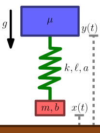
Figure 3: Schematic of vertical hopper. Two masses $m$ and $\mu$, constrained to move vertically above a ground plane in a gravitational field with magnitude $g$, are connected by a linear spring with stiffness $k$ and nominal length $\ell$. The lower mass experiences viscous drag proportional to velocity with constant $b$ when it is in the air, and impacts plastically with the ground (i.e. it is not permitted to penetrate the ground and its velocity is instantaneously set to zero whenever a collision occurs). When the lower mass is in contact with the ground, the spring stiffness is multiplied by a constant $a>1$.

With parameters $(m,\mu,k,b,\ell,a,g)=(1,3,10,5,2,2,2)$, numerical simulations suggest the vertical hopper possesses a stable periodic orbit $\gamma=(y^{*},\dot{y}^{*},x^{*},\dot{x}^{*})$ to which nearby trajectories $(y,\dot{y},x,\dot{x})$ converge asymptotically. Choosing a Poincaré section $\Sigma$ in the ground domain $D_{g}$ at mid-stance, $\Sigma=\left\{(y,\dot{y}):\dot{y}=0\right\}\subset D_{g}$, we find numerically that the hopper possesses a stable periodic orbit $\gamma$ that intersects the Poincaré section at $\gamma\cap\Sigma=\left\{\xi\right\}$ where $\xi=(y,\dot{y})\approx(0.94,0.00)$. Using finite differences, we determine that the linearization $DP$ of the associated scalar–valued Poincaré map $P:\Sigma\rightarrow\Sigma$ has eigenvalue $\operatorname{spec}DP(\xi)\approx 0.57$ at the fixed point $P(\xi)=\xi$. The rank of the Poincaré map $P$ attains the upper bound of Proposition 1, hence Corollary 3 implies the rank hypothesis of Theorem 1 (Exact Reduction) is satisfied. Thus the dynamics of the hopper collapse to a one degree–of–freedom mechanical system after a single hop. Geometrically, the portion of the reduced subsystem in each domain is diffeomorphic to $[0,1]\times\mathbb{R}$. Algebraically, the constraint that activates when the lower mass impacts the ground transfers to the aerial mode where no such physical constraint exists: the lower mass state $(x,\dot{x})$ is uniquely determined by the upper mass state $(y,\dot{y})$ for all future times.

IV-B Reducing a $(3+2n)$ DOF Polyped to a 3 DOF LLS

(a) polyped with $n=4$ legs, leg $k$ annotated

(b) Lateral Leg–Spring (LLS) [17]

Figure 4: Lateral–plane models for locomotion described in Section IV-B.

A primary motivation for the present work is analysis of legged locomotion. Several approaches have been proposed for embedding lower–dimensional dynamics in legged robot systems, notably hybrid zero dynamics [21] and active embedding [25]. Complementing these engineering approaches and predating them, the templates and anchors hypotheses (TAH) [11] conjectures that animal locomotion behaviors arise through reduction of the anchor dynamics governing the nervous system and body [1] to lower–dimensional template dynamics that encode a specific behavior [17, 16]. One well–studied template is the Lateral Leg Spring (LLS) [17] model for sprawled posture running, which has been shown to match how cockroaches run and begin to recover from perturbations [39]. Higher–dimensional neuromechanical variants of the model have been shown to reduce states associated with the nervous system [1]. In this section, we focus on reduction in the mechanical dynamics of limbs. Specifically, we synthesize a state–feedback control law under which the underactuated lateral–plane polyped illustrated in Fig. 4a exactly reduces to the Lateral Leg–Spring (LLS) [17] model in Fig. 4b. With $n$ limbs, the polyped possesses $(3+2n)$ degrees–of–freedom (DOF); the LLS has 3 DOF. This example serves a dual purpose: first, it demonstrates how our theoretical results can be applied to reduce an arbitrary number of DOF in a locomotion model; second, it suggests a mechanism that legged robot controllers could exploit to anchor a desired template.

Before we proceed with describing the reduction procedure in detail, we give an overview of the approach and the connection with Theorem 1. We begin in Section IV-B1 by describing the dynamics of the LLS template and polyped anchor. Then in Section IV-B2 we construct a smooth state feedback law that ensures that trajectories of the polyped body exactly match those of the LLS; we accomplish this by simply ensuring the net wrench [40] comprised of generalized forces and torques acting on the polyped body matches that of the LLS for all time. Subsequently, in Section IV-B3 we modify the feedback law to further ensure the states associated with the polyped’s limbs reduce after a single stride via Theorem 1. Finally, in Section IV-B5 we discuss the effect of perturbations on the closed–loop reduced–order system.

IV-B1 Dynamics of Lateral Leg–Spring (LLS) and $n$–leg polyped

The LLS is an energy–conserving lateral–plane model for locomotion comprised of a massless leg–spring with elastic potential $V$ affixed at hip position $h$ to an inertial body with two translational ($x,y$) and one rotational ($\theta$) DOF. The system is initialized at the start of a stride by orienting the leg at a fixed angle $\beta$ with respect to the body at rest length $\ell$ and touching the foot down such that the leg will instantaneously contract. The step ends once the leg extends to its rest length by touching the foot down on the opposite side of the body; subsequent steps are defined inductively. In certain parameter regimes, the model possesses a periodic running gait [17].

The underactuated hybrid control system illustrated in Fig. 4a extends neuromechanical models previously proposed to study multi–legged locomotion [1, 18] by introducing masses into $n\geq 4$ feet connected by massless limbs affixed at hip locations $\left\{h_{k}\right\}_{k=1}^{n}$ on the inertial body. We assume that each foot can attach or detach from the substrate at any time, and the transition from swing to stance entails a plastic impact that annihilates the kinetic energy in a foot. We assume that each limb $k$ is fully–actuated; for simplicity we assume the inputs act along the Cartesian coordinates and do not saturate so that any $(\mu_{k},\nu_{k})\in\mathbb{R}^{2}$ is feasible at any limb configuration. We let $q_{0}=(x,y,\theta)\in Q_{0}=\mathbb{R}^{2}\times S^{1}$ denote the position and orientation of the body, and for each $k\in\left\{1,\dots,n\right\}$ we let $q_{k}=(x_{k},y_{k})\in Q_{k}\in\mathbb{R}^{2}$ denote the position of the $k$–th foot. The configuration space of the polyped is the $(n+1)$–fold product $\prod_{k=0}^{n}Q_{k}$. The $n$–leg polyped’s dynamics thus have the form

$$M\ddot{q}_{0}=\sum_{k=1}^{n}(-\mu_{k},-\nu_{k},0)\operatorname{Ad}_{g_{k}},\ m_{k}\ddot{q}_{k}=(\mu_{k},\nu_{k})$$ (4)

where $M=\operatorname{diag}\left(m,m,J\right)\in\mathbb{R}^{3\times 3}$ is the mass distribution of the body and $\operatorname{Ad}_{g_{k}}\in\mathbb{R}^{3\times 3}$ transforms a wrench applied at the $k$–th hip to an equivalent wrench applied at the body center–of–mass [40, §5.1].

IV-B2 Embedding LLS in polyped

For any subset $K\subset\left\{1,\dots,n\right\}$ of limbs, let

$$\sum_{k\in K}(-\mu_{k},-\nu_{k},0)\operatorname{Ad}_{g_{k}}\in T^{*}Q_{0}$$ (5)

denote the net wrench [40] on the body resulting from actuating legs in $K$. Then so long as no two hips are coincident and $\left|K\right|\geq 2$, any desired wrench may be imposed on the body by appropriate choice of inputs to the limbs in $K$ regardless of whether $K$ contains limbs in stance or swing. In the next section we describe a limb coordination procedure that ensures there will be a subset of stance limbs that can impose the LLS’s wrench and cancel the reaction wrench from actuating other limbs at any time.

IV-B3 Reducing polyped to LLS

We construct a smooth state feedback control law yielding a closed–loop Poincaré map $P_{A}:U_{A}\rightarrow\Sigma_{A}$ for the polyped that splits as $P_{A}:U_{T}\times U_{N}\rightarrow\Sigma_{T}\times\Sigma_{N}$ such that

$$P_{A}(z,\zeta)=(P_{T}(z),P_{N}(z))$$ (6)

where $P_{T}:U_{T}\rightarrow\Sigma_{T}$ is a Poincaré map for the LLS and $P_{N}:U_{T}\rightarrow\Sigma_{N}$ is a smooth map. In the form (6) it is clear that since $P_{T}$ is a diffeomorphism near the fixed point $\xi=P_{T}(\xi)$, all iterates of $P_{A}$ have constant rank equal to $\operatorname{rank}\,DP_{T}(\xi)=\dim\Sigma_{T}$ near $\xi$, and therefore Theorem 1 applies.

Partition the $n\geq 4$ limbs into $\operatorname{swing}\coprod\operatorname{stance}$, ensuring $\left|\operatorname{swing}\right|$, $\left|\operatorname{stance}\right|\geq 2$. Initialize at the beginning of a step at time $t$ with LLS and polyped body state $(q_{0}(t),\dot{q}_{0}(t))$ and polyped limb states $\left\{(q_{k}(t),\dot{q}_{k}(t))\right\}_{k=1}^{n}$ by attaching $\operatorname{stance}$ limbs and detaching $\operatorname{swing}$ limbs from the ground. Note that the termination time $\tau$ for the LLS step depends smoothly on the initial condition $(q_{0}(t),\dot{q}_{0}(t))$. For each $k\in\operatorname{swing}$ choosing constant inputs

$$\left(\mu_{k},\ \nu_{k}\right)=\frac{2}{\tau^{2}}\left((x(\tau),y(\tau))+r(\theta(\tau))\bar{q}_{k}-q_{k}(t)-\tau\dot{q}_{k}(t)\right)$$ (7)

ensures that the limb will reach a fixed location $\bar{q}_{k}$ in the body frame of reference at time $\tau$. For each $k\in\operatorname{stance}$ choose inputs $(\mu_{k},\nu_{k})$ to cancel the reaction wrench from the swing limbs and impose the LLS acceleration on the polyped body. At time $t+\tau$, exchange the $\operatorname{stance}$ and $\operatorname{swing}$ limb sets and proceed as with the previous step from the new initial condition. After two steps, it is clear that the positions and velocities of the polyped’s $n$ limbs are uniquely determined by the body initial condition $(q_{0}(t),\dot{q}_{0}(t))$. Therefore the polyped’s Poincaré map has the form of (6), so Theorem 1 implies the polyped anchor reduces exactly to the LLS template after a single stride.

IV-B4 Qualitative description of reduction

The active embedding described in Section IV-B2 ensures the polyped body motion is always identical to that of the LLS, regardless of the state of the limbs. The limb posture control in Section IV-B3 guarantees the limb states are determined by the LLS body state after two steps, and furthermore synchronizes touchdown and liftoff events with those of the LLS.

IV-B5 Effect of perturbations and parameter variations

The qualitative description in the preceding section makes it clear that, following a sufficiently small perturbation or parameter variation, the closed–loop polyped will continue to track and ultimately reduce to an LLS that experiences the corresponding disturbance. Note that this conclusion requires that the polyped maintains the same control architecture exploited above to obtain the product decomposition in (6). In particular, the controller must maintain observability of the full state and controllability of the limbs. We study the effect of more general perturbations in the next section.

IV-C Deadbeat Control of Rhythmic Hybrid Systems

Generalizing the example from the previous section, we now consider a system wherein a finitely–parameterized control input updates when an execution passes through a distinguished subset of state space. This form of control in rhythmic hybrid systems dates back (at least) to Raibert’s hoppers [41] and Koditschek’s jugglers [2], and has recently received renewed interest [22, 42, 24, 25, 14, 43, 44]. We model this with a hybrid system $H=(D,F,G,R)$ whose vector field and reset map depend on a control input that takes values in a smooth boundaryless manifold $\Theta$. The value of the control input may be updated whenever an execution passes through the guard $G$, but it does not change in response to the continuous flow. Suppose for some $\theta\in\Theta$ that $H$ possesses a periodic orbit $\gamma$, let $P:U\times\Theta\rightarrow\Sigma$ be a Poincaré map  associated with $\gamma$ where $U\subset\Sigma\subset G$, and let $\left\{\xi\right\}=\gamma\cap\Sigma$. In this section we study deadbeat control of the discrete–time nonlinear control system

$$x_{i+1}=P(x_{i},\theta_{i})$$ (8)

and the discrete–time linear control system obtained by linearizing $P$ about the fixed point $\xi=P(\xi,\theta)$,

$$\delta x_{i+1}=D_{x}P(\xi,\theta)\delta x_{i}+D_{\theta}P(\xi,\theta)\delta\theta_{i}.$$ (9)

The control architecture we present is well–known for linear and nonlinear maps arising in locomotion [22]; the novelty of this section lies in the connection to exact and approximate reduction via Theorems 1 and 2.

IV-C1 Exact reduction over one cycle

As studied in [22], an application of the Implicit Function Theorem [27, Theorem 7.8] shows that if $\operatorname{rank}D_{\theta}P(\xi,\theta)=\dim\Sigma$ then there exists a neighborhood $V\subset U$ of $\xi$ and a smooth feedback law $\psi:V\rightarrow\Theta$ such that for all $x\in V$ we have $P(x,\psi(x))=\xi$, i.e. $\psi$ is a deadbeat control law for (8). Since $\psi$ is smooth, the closed–loop Poincaré map  $P_{\psi}:V\rightarrow\Sigma$ defined by $P_{\psi}(x)=P(x,\psi(x))$ satisfies the hypotheses of Theorem 1 (Exact Reduction) with rank $r=0$, so the invariant subsystem yielded by the Theorem is simply the periodic orbit $\gamma$.

In practice it may be desirable to reduce fewer than $\dim\Sigma$ coordinates. If there exists a smooth function $h:\Sigma\rightarrow\mathbb{R}^{d}$ that satisfies $h\circ P(\xi,\theta)=0$ and $\operatorname{rank}\,D_{\theta}h\circ P(\xi,\theta)=d$, then the preceding construction yields a closed–loop system that reduces via Theorem 1 to the embedded $d$–dimensional submanifold $h^{-1}(0)$ near $\xi$.

IV-C2 Exact reduction over multiple cycles

If $\operatorname{rank}\,D_{\theta}P(\xi,\theta)<\dim\Sigma$, as noted in [22] it may be possible to construct a deadbeat control law by applying inputs over multiple cycles. Specifically, let $P_{0}=P$ and for each $\ell\in\mathbb{N}$ define $P_{\ell}:U_{\ell}\times\Theta^{\ell}\rightarrow\Sigma$ by

$$P_{\ell}(x,(\theta_{1},\dots,\theta_{\ell}))=P(P_{\ell-1}(x,(\theta_{1},\dots,\theta_{\ell-1})),\theta_{\ell})$$ (10)

for all $(x,(\theta_{1},\dots,\theta_{\ell}))\in U_{\ell}\times\Theta^{\ell}$ where $U_{\ell}\subset U$ is a neighborhood of $\xi$ sufficiently small to ensure (10) is well–defined. Then if there exists $k\in\mathbb{N}$ such that

$$\operatorname{rank}\,D_{(\theta_{1},\dots,\theta_{k})}P_{k}(\xi,(\theta,\dots,\theta))=\dim\Sigma,$$ (11)

the construction from the previous paragraph yields a smooth $k$–step feedback law $\psi_{k}:V_{k}\rightarrow\Theta^{k}$ such that the closed–loop hybrid system reduces via Theorem 1 to the periodic orbit $\gamma$ after $k$ cycles. We conclude this section by noting that [22] contains an example that performs exact reduction after two cycles, and for which reduction in fewer cycles is impossible.

IV-C3 Approximate reduction

Since (11) is equivalent to controllability [34, Chapter 8d.5] of the linear control system (9), it is worthwhile to consider the linear control problem. Any stabilizable subspace $S$ [34, Chapter 8d.7] of (9) can be rendered attracting in a finite number of steps $k\in\mathbb{N}$ with linear state feedback $\delta\theta_{i}=\Psi\delta x_{i}$ where $\Psi$ is a fixed matrix [45]. Applying this linear feedback law to the nonlinear system (8) yields a closed–loop Poincaré map $P_{\Psi}$ such that the rangespace of the $k$–th iterate of its linearization $D_{x}P^{k}_{\Psi}(\xi)$ is contained in $S$. Therefore Theorem 2 (Approximate Reduction) yields an invariant hybrid subsystem, tangent to $S$ on $\Sigma$, that attracts nearby trajectories superexponentially. Thus, although feedback laws for the nonlinear control system (8) constructed above can be computed using the procedure described in [22] to achieve exact reduction to the target subsystem, if approximate reduction suffices then one may simply apply the linear deadbeat controller computed for (9).

IV-C4 Structural stability of deadbeat control

Suppose the preceding development is applied to a model that differs from that used to construct the feedback law $\psi\in C^{\infty}(V,\Theta)$. We study the structural stability [31, Section 1.7] of attracting invariant sets arising in this class of systems by applying the Theorems of Section III. If the models differ by a small smooth deformation (as would occur if there was a small perturbation in model parameters), one interpretation of this change is that some $\widetilde{\psi}\in B_{\varepsilon}(\psi)\subset C^{\infty}(V,\Theta)$ is applied to the model for which $\psi$ is deadbeat, where $\varepsilon>0$ bounds the error. For all $\varepsilon>0$ sufficiently small, $\widetilde{\psi}$ yields a perturbed closed–loop Poincaré map  $\widetilde{P}:V\rightarrow\Sigma$ possessing a unique fixed point $\widetilde{\xi}\in V$, and $\widetilde{\xi}$ is an exponentially stable fixed point of the perturbed system.

We conclude by noting that it is possible for the structure of the hybrid dynamics to constrain the achievable perturbations. For instance, if one domain of the hybrid system has lower dimension than that in which the Poincaré map  is constructed, then zero is always a Floquet multiplier regardless of the applied feedback; in this case Theorem 2 (Approximate Reduction) implies the existence of a proper submanifold of the Poincaré section $\Sigma$ to which trajectories contract superexponentially in the presence of any (sufficiently small) smooth perturbation to the closed–loop dynamics.

IV-D Hybrid Floquet Coordinates

When a hybrid system reduces to a smooth dynamical system near a periodic orbit via Theorem 1 (Exact Reduction), we can generalize the Floquet normal form [46, 47, 48, 49] using Theorem 3 (Smoothing). Broadly, this demonstrates how the Theorems of Section III can be applied to generalize constructions from classical dynamical systems theory to the hybrid setting. More concretely, this provides a theoretical framework that justifies application of the empirical approach developed in [48, 49] to estimate low–dimensional invariant dynamics in data collected from physical locomotors.

Consider a hybrid dynamical system $H=(D,F,G,R)$ with $\tau$–periodic orbit $\gamma$ that satisfies the hypotheses of Theorem 1. Let $M\subset D$ be the $(r+1)$–dimensional invariant hybrid subsystem yielded by the Theorem, and $W\subset D$ a hybrid open set containing $\gamma$ that contracts to $M$ in finite time. Let $(\widetilde{M},\widetilde{F})$ denote the smooth dynamical system obtained by applying Theorem 3. Under a genericity condition there exists a neighborhood $U\subset\widetilde{M}$ of $\gamma$ and a smooth chart $\varphi:U\rightarrow\mathbb{R}^{r}\times S^{1}$ such that the coordinate representation of the vector field has the form

$$D\varphi\circ\widetilde{F}\circ D\varphi^{-1}(z,\theta)=\left(\begin{array}[]{c}\dot{z}\\ \dot{\theta}\end{array}\right)=\left(\begin{array}[]{c}A(\theta)z\\ 2\pi/\tau\end{array}\right)$$ (12)

where $z\in\mathbb{R}^{r}$ and $\theta\in S^{1}$. In these coordinates, each $\theta\in S^{1}$ determines an embedded submanifold $\widetilde{N}_{\theta}=\mathbb{R}^{r}\times\left\{\theta\right\}\subset\mathbb{R}^{r}\times S^{1}$ that is mapped to itself after flowing forward in time by $\tau$; for this reason, the submanifolds $\widetilde{N}_{\theta}$ are referred to as isochrons [47]. Each $x\in\widetilde{N}_{\theta}$ may be assigned the phase $\theta\in S^{1}$; if $\gamma$ is stable, then as $t\rightarrow\infty$ the trajectory initialized at $x$ will asymptotically converge to the trajectory initialized at $(0,\theta)$.

The isochrons may be pulled back to any precompact hybrid open set $V\subset W$ containing $\gamma$ in the original hybrid system as follows. The proof of Theorem 1 implies there exists a finite time $t<\infty$ such that every execution initialized in $V$ is defined over the time interval $[0,t]$ and reaches $M$ before time $t$; without loss of generality, we take this time to be a multiple $k\tau$ of the period of $\gamma$ for some $k\in\mathbb{N}$. Let $\psi:V\rightarrow\widetilde{M}$ denote the map that flows an initial condition $x\in V$ forward by $t$ time units and then applies the quotient projection $\pi:M\rightarrow\widetilde{M}$ obtained from Theorem 3 to yield the point $\psi(x)\in\widetilde{M}$. Then the constructions in the proof of Theorem 1 imply that $\psi$ is a smooth map in the sense defined in Section III-A, i.e. it is continuous and $\psi|_{V\cap D_{j}}$ is smooth for each $j\in J$. Now for any $\theta\in S^{1}$ the set $N_{\theta}=\psi^{-1}(U)$ is mapped into $\widetilde{N}_{\theta}$ after $k\tau$ units of time; we thus refer to $N_{\theta}\subset D$ as a hybrid isochron. We conclude by noting that $N_{\theta}$ will generally not be a smooth (hybrid) submanifold.

V Discussion

Generically for an exponentially stable periodic orbit in a hybrid dynamical system, nearby trajectories contract superexponentially to a subsystem containing the orbit. Under a non–degeneracy condition on the rank of any Poincaré map  associated with the orbit, this contraction occurs in finite time regardless of the stability of the orbit. Hybrid transitions may be removed from the resulting subsystem, yielding an equivalent smooth dynamical system. Thus the dynamics near stable hybrid periodic orbits are generally obtained by extending the behavior of a smooth system in transverse coordinates that decay superexponentially. Although the applications presented in Section IV focused on terrestrial locomotion [1], we emphasize that the results in Section III do not depend on the phenomenology of the physical system under investigation, and are hence equally suited to study rhythmic hybrid control systems appearing in robotic manipulation [2], biochemistry [3], and electrical systems [4].

In addition to providing a canonical form for the dynamics near hybrid periodic orbits, the results of this paper suggest a mechanism by which a many–legged locomotor or a multi–fingered manipulator may collapse a large number of mechanical degrees–of–freedom to produce a low–dimensional coordinated motion. This provides a link between disparate lines of research: formal analysis of hybrid periodic orbits; design of robots for rhythmic locomotion and manipulation tasks; and scientific probing of neuromechanical control architectures in humans and animals. Our theoretical results show that hybrid models of rhythmic phenomena generically reduce dimensionality, and our applications demonstrate that this reduction may be deliberately designed into an engineered system. We furthermore speculate that evolution may have exploited this reduction in developing its spectacularly dexterous agents.

Support

This research was supported in part by: an NSF Graduate Research Fellowship to S. A. Burden; ARO Young Investigator Award #61770 to S. Revzen; and Army Research Laboratory Cooperative Agreements W911NF–08–2–0004 and W911NF–10–2–0016. The views and conclusions contained in this document are those of the authors and should not be interpreted as representing the official policies, either expressed or implied, of the Army Research Laboratory or the U.S. Government. The U.S. Government is authorized to reproduce and distribute for Government purposes notwithstanding any copyright notation herein.

Acknowledgments

We thank John Hauser for correcting an error in an earlier version of this manuscript, and Sam Coogan, John Guckenheimer, Ram Vasudevan, and the three anonymous reviewers for their invaluable feedback.

Appendix A Smooth Dynamical Systems

We constructed hybrid systems using switching maps defined on boundaries of smooth dynamical systems. The behavior of such systems can be studied by alternately applying flows and maps, thus in this section we collect results that provide canonical forms for the behavior of flows and maps near periodic orbits and fixed points, respectively. The first develops a canonical form for the flow to a section in a continuous–time system. The second provides a technique to smoothly attach continuous–time systems along their boundaries. The third and fourth establish a canonical form for submanifolds that are invariant and approximately invariant (respectively) near fixed points in discrete–time dynamical systems; the fifth provides an estimate of the error in the invariance approximation.

A-A Continuous–Time Dynamical Systems

Definition 4.

A continuous–time dynamical system is a pair $(M,F)$ where:

• is a smooth manifold with boundary $\partial M$;

• is a smooth vector field on $M$, i.e. $F\in\mathscr{T}(M)$.

A-A1 Time–to–Impact

When a trajectory passes transversely through an embedded submanifold, the time required for nearby trajectories to pass through the manifold depends smoothly on the initial condition [30, Chapter 11.2]. This provides the prototype used in the proofs of Theorems 1 and 2 for the dynamics near the portion of a hybrid periodic orbit in one domain of a hybrid system.

Lemma 2.

Let $(M,F)$ be a smooth dynamical system, $\phi:\mathscr{F}\rightarrow M$ the maximal flow associated with $F$, and $G\subset M$ a smooth codimension–1 embedded submanifold. If there exists $x\in M$ and $t\in\mathscr{F}^{x}$ such that $\phi(t,x)\in G$ and $F\left(\phi(t,x)\right)\not\in T_{{\normalsize{{{\phi(t,x)}}}}}G$, then there is a neighborhood $U\subset M$ containing $x$ and a smooth map $\sigma:U\rightarrow\mathbb{R}$ so that $\sigma(x)=t$ and $\phi(\sigma(y),y)\in G$ for all $y\in U$; $\sigma$ is called the time–to–impact map.

Proof.

Near $\phi(t,x)$, $G$ is the zero section of a constant–rank map $h:M\rightarrow\mathbb{R}$ where $Dh\left(\phi(t,x)\right)\neq 0$. Define $g:\mathscr{F}\rightarrow\mathbb{R}$ by $g(s,y)=(h\circ\phi)(s,y)$. Then since $F$ is transverse to $G$ at $\phi(t,x)$,

$$\frac{\partial g}{\partial t}(t,x)=Dh\left(F\left(\phi(t,x)\right)\right)\neq 0.$$

By the Implicit Function Theorem (see Theorem 7.8 in [27]), there exists a neighborhood $U$ of $x$ and a smooth map $\sigma:U\rightarrow\mathbb{R}$ so that $\sigma(x)=t$ and $g(\sigma(y),y)=0$ for all $y\in U$, i.e. $\phi(\sigma(y),y)\in G$. ∎

Remark 5.

This lemma is applicable when $G\subset\partial M$.

A-A2 Smoothing Flows

Two continuous–time dynamical systems can be smoothly attached to one another along their boundaries to obtain a new continuous–time system [26, Theorem 8.2.1]. Distinct hybrid domains were attached to one another using this construction in Section III.

Lemma 3.

Suppose $(M_{1},F_{1}),(M_{2},F_{2})$ are $n$–dimensional continuous–time dynamical systems, there exists a diffeomorphism $R:\partial M_{1}\rightarrow\partial M_{2}$, $F_{1}$ is outward–pointing along $\partial M_{1}$, and $F_{2}$ is inward–pointing along $\partial M_{2}$. Then the topological quotient

$$\widetilde{M}=\frac{M_{1}\coprod M_{2}}{\partial M_{1}\overset{R}{\sim}\partial M_{2}}$$

can be endowed with the structure of a smooth manifold such that for $j\in\left\{1,2\right\}$:

1. the quotient projections $\pi_{j}:M_{j}\rightarrow\widetilde{M}$ are smooth embeddings; and

2. there is a smooth vector field $\widetilde{F}\in\mathscr{T}(\widetilde{M})$ that restricts to $D\pi_{j}(F_{j})$ on $\pi(M_{j})\subset\widetilde{M}$.

Proof.

Let $\phi_{j}:\mathscr{F}_{j}\rightarrow M_{j}$ be the maximal flow associated with $F_{j}$ on $M_{j}$. Then there is a neighborhood $\widetilde{U}_{j}\subset\mathscr{F}_{j}$ of $\left\{0\right\}\times M_{j}$ on which the flow is defined, and with $U_{j}=\widetilde{U}_{j}\cap(\mathbb{R}\times\partial M_{j})$, transversality of $F_{j}$ along $\partial M_{j}$ implies $\phi_{j}:U_{j}\rightarrow M_{j}$ is an embedding which is the identity on $\left\{0\right\}\times\partial M_{j}$. Since $F_{1}$ is outward–pointing and $F_{2}$ is inward–pointing, the neighborhoods are one–sided and without loss of generality we may assume for $j=1,2$ that there exist continuous positive functions $\delta_{j}:\partial M_{j}\rightarrow[0,\infty)$ such that $U_{1}=\left\{(-\delta_{1}(x),0]:x\in\partial M_{1}\right\}$ and $U_{2}=\left\{[0,\delta_{2}(x)):x\in\partial M_{2}\right\}$. Therefore $U=\frac{U_{1}\coprod U_{2}}{\partial M_{1}\simeq\partial M_{2}}$ inherits a smooth structure from its product structure, i.e. the fibers $U^{x}=(-\delta_{1}(x),\delta_{2}(\varphi(x)))\times\left\{x\right\}$ are smooth curves for $x\in\partial M_{1}$ and both $\left\{0\right\}\times\partial M_{1}\hookrightarrow U$ and $\left\{0\right\}\times\varphi^{-1}(\partial M_{2})\hookrightarrow U$ are smooth embeddings; let $\varphi:U\rightarrow\mathbb{R}^{n}$ denote the chart. Note in addition that by construction the constant vector field $\frac{\partial\ }{\partial t}\in\mathscr{T}(U_{j})$ pushes forward to $F_{j}|_{\phi_{j}(U_{j})\cap M_{j}}\in\mathscr{T}\left(\phi_{j}(U_{j})\cap M_{j}\right)$, since $(D\phi_{j})\frac{\partial\ }{\partial t}=F_{j}$.

We construct the smooth structure on $\widetilde{M}=\frac{M_{1}\coprod M_{2}}{\partial M_{1}\simeq\partial M_{2}}$ by covering $M$ with interior charts from the $M_{j}$’s together with $U$. Note that since $\phi_{j}|_{U_{j}}:U_{j}\rightarrow M_{j}$ is a smooth embedding, the interior charts on $M_{j}$ are smoothly compatible with the product chart on $U$, and the natural quotient projections $\pi_{j}:M_{j}\hookrightarrow\widetilde{M}$ are smooth embeddings. Finally, $(D\pi_{1})F_{1}=(D\pi_{2})F_{2}$ along $\pi_{1}(\partial M_{1})$ by construction, whence the vector field $\widetilde{F}\in\mathscr{T}(\widetilde{M})$ which restricts to $F_{j}$ on $M_{j}$, $j=1,2$, is well–defined and smooth. ∎

Remark 6.

The smooth structure constructed in Lemma 3 is unique up to diffeomorphism [26, Theorem 2.1 in Chapter 8].

A-B Discrete–time Dynamical Systems

Definition 5.

A discrete–time dynamical system is a pair $(\Sigma,P)$ where:

• is a smooth manifold without boundary;

• is a smooth endomorphism of $\Sigma$, i.e. $P:\Sigma\rightarrow\Sigma$.

In studying hybrid dynamical systems, we encounter smooth maps $P:\Sigma\rightarrow\Sigma$ that are noninvertible. Viewing iteration of $P$ as determining a discrete–time dynamical system, we wish to study the behavior of these iterates near a fixed point $\xi=P(\xi)$. Note that if $P$ has constant rank equal to $k<n=\dim\Sigma$, then its image $P(\Sigma)\subset\Sigma$ is an embedded $k$–dimensional submanifold near $\xi$ by the Rank Theorem [27, Theorem 7.13]. With an eye toward model reduction, one might hope that the composition $(P\circ P):\Sigma\rightarrow P(\Sigma)$ is also constant–rank, but this is not generally true.

In this section we provide three results that introduce regularity into iterates of a noninvertible map $P:\Sigma\rightarrow\Sigma$ on an $n$–dimensional manifold $\Sigma$ near a fixed point $P(\xi)=\xi$. If the rank of $DP$ is strictly bounded above by $m\in\mathbb{N}$ and if $P^{m}$, the $m$–th iterate of $P$, has constant rank equal to $r\in\mathbb{N}$ near the fixed point $\xi$, then $P$ reduces to a diffeomorphism over an $r$–dimensional invariant submanifold after $m$ iterations; this result is given in Section A-B1. Even if $DP^{m}$ is not constant rank, as long as $\xi$ is exponentially stable then $P$ can be approximated by a diffeomorphism on a submanifold whose dimension equals $\operatorname{rank}\,DP^{m}(\xi)$; this is the subject of Section A-B2. A bound on the error in this approximation is provided in Section A-B3.

A-B1 Exact Reduction

If the rank of $P:\Sigma\rightarrow\Sigma$ is strictly bounded above by $m\in\mathbb{N}$ and the derivative of the $m$–th iterate of $P$ has constant rank near a fixed point, then the range of $P$ is locally an embedded submanifold, and $P$ restricts to a diffeomorphism over that submanifold. This originally appeared without proof as Lemma 3 in [33].

Lemma 4.

Let $(\Sigma,P)$ be an $n$–dimensional discrete–time dynamical system with $P(\xi)=\xi$ for some $\xi\in\Sigma$. Suppose the rank of $P$ is strictly bounded above by $m\in\mathbb{N}$ and there exists a neighborhood $W\subset\Sigma$ of $\xi$ such that $\operatorname{rank}\,DP^{m}(x)=r$ for all $x\in W$. Then there is a neighborhood $V\subset\Sigma$ containing $\xi$ such that $P^{m}(V)$ is an $r$–dimensional embedded submanifold near $\xi$ and there is a neighborhood $U\subset P^{m}(V)$ containing $\xi$ that $P$ maps diffeomorphically onto $P(U)\subset P^{m}(V)$.

In the proof of Lemma 4, we make use of a fact from linear algebra obtained by passing to the Jordan canonical form.

Proposition 2.

If $A\in\mathbb{R}^{n\times n}$ and $\operatorname{rank}A<m$, then $\operatorname{rank}(A^{2m})=\operatorname{rank}(A^{m})$.

Proof.

(of Lemma 4) By the Rank Theorem [27, Theorem 7.13], there is a neighborhood $V\subset\Sigma$ of $\xi$ for which $S=P^{m}(V)$ is an $r$–dimensional embedded submanifold and by Proposition 2 we have

$$\operatorname{rank}\left(DP^{m}|_{S}\right)(\xi) =\operatorname{rank}D(P^{m}\circ P^{m})(\xi)$$

$$=\operatorname{rank}DP^{m}(\xi).$$

Therefore $DP^{m}|_{S}:T_{\xi}S\rightarrow T_{\xi}S$ is a bijection, so by the Inverse Function Theorem [27, Theorem 7.10], there is a neighborhood $W\subset S$ containing $\xi$ so that $P^{m}(W)\subset S$ and $P^{m}|_{W}:W\rightarrow P^{m}(W)$ is a diffeomorphism.

We now show that $W$ is invariant under $P$ in a neighborhood of $\xi$. By continuity of $P$, there is a neighborhood $L\subset V$ containing $\xi$ for which $P(L)\subset V$ and $P^{m}(L)\subset W$. The set $U=P^{m}(L)$ is a neighborhood of $\xi$ in $S$. Further, we have

$$P(U) =P\circ P^{m}(L)=P^{m}\circ P(L)\subset S.$$

The restriction $P^{m}|_{U}:U\rightarrow P^{m}(U)$ is a diffeomorphism since $U\subset W$, whence $P|_{U}$ is a diffeomorphism onto its image $P(U)\subset S$. ∎

A-B2 Approximate Reduction

Now suppose that iterates of $P$ are not constant rank but $\xi=P(\xi)$ is exponentially stable, meaning that the spectral radius $\rho\left(DP(\xi)\right)=\max\left\{\left|\lambda\right|:\lambda\in\operatorname{spec}DP(\xi)\right\}$ satisfies $\rho\left(DP(\xi)\right)<1$. We show that $P$ may be approximated by a diffeomorphism defined on a submanifold whose dimension equals the number of non–zero eigenvalues of $DP(\xi)$. The technical result we desire was originally established by Hartman [50]. We apply Hartman’s Theorem to construct a $C^{1}$ change–of–coordinates that exactly linearizes all eigendirections corresponding to non–zero eigenvalues of $DP(\xi)$.

Lemma 5.

Let $(\Sigma,P)$ be an $n$–dimensional discrete–time dynamical system. Suppose $\xi=P(\xi)$ is an exponentially stable fixed point and let $r$ be the number of non–zero eigenvalues of $DP(\xi)$. Then there is a neighborhood $U\subset\Sigma$ of $\xi$ and a $C^{1}$ diffeomorphism $\varphi:U\rightarrow\mathbb{R}^{n}$ such that $\varphi(\xi)=0$ and the coordinate representation $\widetilde{P}=\varphi\circ P\circ\varphi^{-1}$ of $P$ has the form

$$\widetilde{P}(z,\zeta)=\left(Az,\ N(z,\zeta)\right)$$

where $z\in\mathbb{R}^{r}$, $\zeta\in\mathbb{R}^{n-r}$, $A\in\mathbb{R}^{r\times r}$ is invertible, $N:\varphi(U)\rightarrow\mathbb{R}^{n-r}$ is $C^{1}$, $N(0,0)=0$, and $D_{\zeta}N(0,0)$ is nilpotent.

Proof.

Let $(U_{0},\varphi_{0})$ be a smooth chart for $\Sigma$ with $\xi\in U_{0}$ and $\varphi_{0}(\xi)=0$. We begin by verifying that the hypotheses of Theorem 4 from Appendix B are satisfied for the map $P_{0}:\varphi_{0}(U_{0})\rightarrow\mathbb{R}^{n}$ defined by $P_{0}=\varphi_{0}\circ P\circ\varphi_{0}^{-1}$. Let $\lambda\in\operatorname{spec}DP_{0}(0)$ be the eigenvalue with largest magnitude, and $\ell\in\mathbb{N}$ its algebraic multiplicity. Applying the linear change–of–coordinates that puts $DP_{0}(0)$ into Jordan canonical form, we assume

$$DP_{0}(0) =\left(\begin{array}[]{ccc}A&0\\ 0&B\end{array}\right)$$

where $B\in\mathbb{R}^{\ell\times\ell}$ and $\operatorname{spec}B=\left\{\lambda\right\}$. Now in the notation of Theorem 4,

$$P_{0}(x,y)=\left(Ax+X(x,y),By+Y(x,y)\right)$$

where $x\in\mathbb{R}^{n-\ell}$, $y\in\mathbb{R}^{\ell}$, and $X$, $Y$ are smooth and $X(0,0)=0$, $Y(0,0)=0$; note that $m=0$ (there is no $z$ coordinate) at this step. Because $X$ and $Y$ are smooth on the neighborhood $U_{0}$ of the origin, their derivatives are uniformly Lipschitz and Hölder continuous on a precompact open subset of $U_{0}$.

Theorem 4 implies there exists a neighborhood $U_{1}\subset\mathbb{R}^{n}$ of the origin and a $C^{1}$ diffeomorphism $\varphi_{1}:U_{1}\rightarrow\mathbb{R}^{n}$ for which the map $P_{1}:\varphi_{1}(U_{1})\rightarrow\mathbb{R}^{n}$ defined by $P_{1}=\varphi_{1}\circ P_{0}\circ\varphi_{1}^{-1}$ has the form (after reversing the order of the coordinates)

$$P_{1}(z_{1},\zeta_{1})=\left(A_{1}z_{1},\ N_{1}(z_{1},\zeta_{1})\right)$$

where $z_{1}\in\mathbb{R}^{r_{1}}$, $r_{1}>0$, $\zeta_{1}\in\mathbb{R}^{n-r_{1}}$ and $A_{1}\in\mathbb{R}^{r_{1}\times r_{1}}$ is invertible. Observe that the map $P_{1}$ satisfies the hypotheses of Theorem 4. Therefore we may inductively apply the Theorem to construct a sequence of coordinate charts $\left\{(U_{k},\varphi_{k})\right\}_{k=1}^{K}$ and corresponding maps $\left\{P_{k}\right\}_{k=1}^{K}$ such that for all $k\in\left\{1,\dots,K\right\}$

$$P_{k}(z_{k},\zeta_{k})=\left(A_{k}z_{k},\ N_{k}(z_{k},\zeta_{k})\right)$$

where $z_{k}\in\mathbb{R}^{r_{k}}$, $\zeta_{k}\in\mathbb{R}^{n-r_{k}}$, $A_{k}\in\mathbb{R}^{r_{k}\times r_{k}}$ is invertible, and $r_{k}>r_{k-1}$ (note that $r_{0}=0$). The sequence terminates at a finite $K<\infty$ with $r_{K}=r=\operatorname{rank}DP^{n}(\xi)$. Therefore in the $C^{1}$ chart $(U,\varphi)$ given by $\varphi=\varphi_{K}\circ\cdots\circ\varphi_{0}$ and $U=\varphi^{-1}(\mathbb{R}^{n})$, the coordinate representation $\widetilde{P}=\varphi\circ P\circ\varphi^{-1}$ of $P$ has the form

$$\widetilde{P}(z,\zeta)=\left(Az,\ N(z,\zeta)\right)$$

where $z\in\mathbb{R}^{r}$, $\zeta\in\mathbb{R}^{n-r}$ and $A\in\mathbb{R}^{r\times r}$ is invertible. Since $A$ is invertible and $\operatorname{rank}D\widetilde{P}^{n}(\xi)=r$, $D_{\zeta}N(0,0)$ is nilpotent. ∎

A-B3 Superstability

Finally, we recall that if all eigenvalues of the linearization of a map at a fixed point are zero—a so–called “superstable” fixed point [28]—then the map contracts superexponentially; this is a straightforward consequence of Ostrowski’s Theorem [53, 8.1.7].

Lemma 6.

Let $P:\mathbb{R}^{n}\rightarrow\mathbb{R}^{n}$ be a $C^{1}$ map with $P(0)=0$, $\operatorname{spec}DP(0)=\left\{0\right\}$. Then for every $\varepsilon>0$ and norm $\left\|\cdot\right\|:\mathbb{R}^{n}\rightarrow\mathbb{R}$ there exists $\delta,C>0$ such that

$$\forall x\in B_{\delta}(0),k\in\mathbb{N}:\left\|P^{k}(x)\right\|\leq C\varepsilon^{k}\left\|x\right\|.$$

The proof of Lemma 6 relies on the following elementary fact regarding induced norms [53, 1.3.6].

Proposition 3 (1.3.6 in [53]).

Given $\varepsilon>0$ and $A\in\mathbb{R}^{n\times n}$, there exists a norm $\left\|\cdot\right\|:\mathbb{R}^{n}\rightarrow\mathbb{R}$ such that $\left\|A\right\|_{i}\leq\rho\left(A\right)+\varepsilon$, where $\left\|\cdot\right\|_{i}:\mathbb{R}^{n\times n}\rightarrow\mathbb{R}$ is the operator norm induced by $\left\|\cdot\right\|$ and $\rho(A)$ is the spectral radius of $A$.

Proof.

(of Lemma 6) Given $\varepsilon>0$, choose the norm $\left\|\cdot\right\|:\mathbb{R}^{n}\rightarrow\mathbb{R}$ obtained by applying Proposition 3 to $DP(0)$ so that $\left\|DP(0)\right\|_{i}\leq\frac{1}{2}\varepsilon$. Since $DP$ is continuous, there exists a $\delta>0$ such that

$$\forall x\in B_{\delta}(0):\left\|DP(x)-DP(0)\right\|_{i}<\frac{1}{2}\varepsilon.$$

Whence we find for $\left\|x\right\|<\delta$ that

$$\left\|DP(x)\right\|_{i} =\left\|DP(x)-DP(0)+DP(0)\right\|_{i}$$

$$\leq\left\|DP(x)-DP(0)\right\|_{i}+\left\|DP(0)\right\|_{i}\leq\varepsilon.$$

Combined with 8.1.4 in [53] (a generalization of the Mean Value Theorem to vector–valued functions), we find for all $x\in B_{\delta}(0)$,

$$\left\|P(x)\right\| \leq\sup_{s\in[0,1]}\left\|DP(sx)\right\|_{i}\left\|x\right\|\leq\varepsilon\left\|x\right\|.$$

Iterating, for all $k\in\mathbb{N}$ and $\left\|x\right\|<\delta$ we have $\left\|P^{k}(x)\right\|\leq\varepsilon^{k}\left\|x\right\|$. Since all norms on finite–dimensional vector spaces are equivalent, the desired result follows immediately. ∎

Remark 7.

Let $(\Sigma,P)$ be an $n$–dimensional discrete–time dynamical system that satisfies the hypotheses of Lemma 5 near $\xi=P(\xi)$. Then $P$ has a coordinate representation $\widetilde{P}(z,\zeta)=\left(Az,N(z,\zeta)\right)$ in a neighborhood of $\xi$ where $A$ is an invertible matrix, $N(0,0)=0$, and $\operatorname{spec}D_{\zeta}N(0,0)=\left\{0\right\}$. Therefore given $\varepsilon>0$ we can apply Lemma 6 to the nonlinearity $\widetilde{P}(z,\zeta)-\left(Az,0\right)=\left(0,N(z,\zeta)\right)$ to find $\delta,C>0$ such that for all $\left(z,\zeta\right)\in B_{\delta}(0)$ and $k\in\mathbb{N}$:

$$\left\|\widetilde{P}^{k}(z,\zeta)-\left(A^{k}z,0\right)\right\|\leq C\varepsilon^{k}\left\|\left(z,\zeta\right)\right\|.$$

We conclude that $P$ is arbitrarily well–approximated near $\xi$ by a diffeomorphism on a submanifold whose dimension equals $\operatorname{rank}DP^{n}(\xi)$.

Appendix B $C^{1}$ Linearization

The technical result we desire was originally established by Hartman in the course of proving that an invertible contraction is $C^{1}$–conjugate to its linearization. The original statement in [50] only considered invertible contractions. However, as noted in [51], the proof in [50] of the result we require does not make use of invertibility and the conclusion is still valid if zero is an eigenvalue of the linearization. For details we refer the reader to [52], which also contains a generalization to hyperbolic periodic orbits whose eigenvalues satisfy genericity conditions.

Theorem 4 (Induction Assertion in [50]).

Let $U\subset\mathbb{R}^{n}$ be a neighborhood of the origin and $P:U\rightarrow\mathbb{R}^{n}$ a $C^{1}$ map of the form

$$P(x,y,z) =\left(Ax+X(x,y,z),\ By+Y(x,y,z),\ Cz\right)$$

such that

$$DP(0) =\left(\begin{array}[]{ccc}A&0&0\\ 0&B&0\\ 0&0&C\end{array}\right)$$

where:

1. $x\in\mathbb{R}^{k}$, $y\in\mathbb{R}^{\ell}$, $z\in\mathbb{R}^{m}$ and $k+\ell+m=n$;

2. $A\in\mathbb{R}^{k\times k}$, $B\in\mathbb{R}^{\ell\times\ell}$, and $C\in\mathbb{R}^{m\times m}$;

3. $X:\mathbb{R}^{n}\rightarrow\mathbb{R}^{k}$ and $Y:\mathbb{R}^{n}\rightarrow\mathbb{R}^{\ell}$ are $C^{1}$;

4. $D_{x}X$, $D_{y}X$, $D_{x}Y$, and $D_{y}Y$ are uniformly Lipschitz continuous in $(x,y)$;

5. $D_{z}X$ and $D_{z}Y$ are uniformly Hölder continuous in $z$;

Suppose all the eigenvalues of $B$ have the same magnitude, that the eigenvalues of $A$ have smaller magnitude and those of $C$ have larger magnitude than those of $B$, and all eigenvalues of $DP(0)$ lie inside the unit disc:

$$\forall b,\beta\in\operatorname{spec}B :\left|b\right|=\left|\beta\right|;$$

$$\forall a\in\operatorname{spec}A,b\in\operatorname{spec}B,c\in\operatorname{spec}C :0\leq\left|a\right|<\left|b\right|<\left|c\right|<1.$$

Then there is a neighborhood of the origin $V\subset\mathbb{R}^{n}$ and a $C^{1}$ diffeomorphism $\varphi:V\rightarrow\mathbb{R}^{n}$ of the form

$$\varphi(x,y,z) =\left(x+\varphi_{X}(z),\ y+\varphi_{Y}(x,y,z),\ z\right)$$

for which $D\varphi(0)=I$ and for all $(u,v,w)\in\varphi(V)$ we have

$$(\varphi\circ P\circ\varphi^{-1})(u,v,w)=\left(Au+U(u,v,w),\ Bv,\ Cw\right)$$

where:

1. $U:\varphi(V)\rightarrow\mathbb{R}^{k}$ is $C^{1}$;

2. $D_{u}U$ is uniformly Lipschitz continuous in $(u,v,w)$;

3. $D_{v}U$ and $D_{w}U$ are uniformly Lipschitz continuous in $u$;

4. $D_{v}U$ and $D_{w}U$ are uniformly Hölder continuous in $(v,w)$.

Remark 8.

Theorem 4 may be applied inductively to exactly linearize all eigendirections corresponding to non–zero eigenvalues via a $C^{1}$ change–of–coordinates; this is the content of Lemma 5 in Section A-B2.

References

- [1] P. Holmes, R. J. Full, D. E. Koditschek, and J. M. Guckenheimer, “The dynamics of legged locomotion: Models, analyses, and challenges,” SIAM Review, vol. 48, no. 2, pp. 207–304, 2006.
- [2] M. Buehler, D. E. Koditschek, and P. J. Kindlmann, “Planning and control of robotic juggling and catching tasks,” The International Journal of Robotics Research, vol. 13, no. 2, pp. 101–118, 1994.
- [3] L. Glass and J. S. Pasternack, “Stable oscillations in mathematical models of biological control systems,” Journal of Mathematical Biology, vol. 6, no. 3, pp. 207–223, 1978.
- [4] I. A. Hiskens and P. B. Reddy, “Switching–induced stable limit cycles,” Nonlinear Dynamics, vol. 50, no. 3, pp. 575–585, 2007.
- [5] J. Lygeros, K. H. Johansson, S. N. Simic, J. Zhang, and S. S. Sastry, “Dynamical properties of hybrid automata,” IEEE Transactions on Automatic Control, vol. 48, no. 1, pp. 2–17, 2003.
- [6] S. Grillner, “Neurobiological bases of rhythmic motor acts in vertebrates,” Science, vol. 228, pp. 143–149, 1985.
- [7] A. Cohen, P. J. Holmes, and R. H. Rand, “The nature of coupling between segmental oscillators of the lamprey spinal generator for locomotion: a model,” Journal of Mathematical Biology, vol. 13, pp. 345–369, 1982.
- [8] M. Golubitsky, I. Stewart, P. L. Buono, and J. J. Collins, “Symmetry in locomotor central pattern generators and animal gaits,” Nature, vol. 401, no. 6754, pp. 693–695, 1999.
- [9] L. H. Ting and J. M. Macpherson, “A limited set of muscle synergies for force control during a postural task,” Journal of Neurophysiology, vol. 93, no. 1, pp. 609–613, 2005.
- [10] C. Li, T. Zhang, and D. I. Goldman, “A terradynamics of legged locomotion on granular media,” Science, vol. 339, no. 6126, pp. 1408–1412, 2013.
- [11] R. J. Full and D. E. Koditschek, “Templates and anchors: Neuromechanical hypotheses of legged locomotion on land,” Journal of Experimental Biology, vol. 202, pp. 3325–3332, 1999.
- [12] T. McGeer, “Passive dynamic walking,” International Journal of Robotics Research, vol. 9, no. 2, p. 62, 1990.
- [13] J. W. Grizzle, G. Abba, and F. Plestan, “Asymptotically stable walking for biped robots: Analysis via systems with impulse effects,” IEEE Transactions on Automatic Control, vol. 46, no. 1, pp. 51–64, 2002.
- [14] A. Seyfarth, H. Geyer, and H. Herr, “Swing–leg retraction: a simple control model for stable running,” Journal of Experimental Biology, vol. 206, no. 15, pp. 2547–2555, 2003.
- [15] S. Collins, A. Ruina, R. Tedrake, and M. Wisse, “Efficient bipedal robots based on passive–dynamic walkers,” Science, vol. 307, no. 5712, pp. 1082–1085, 2005.
- [16] R. M. Ghigliazza, R. Altendorfer, P. Holmes, and D. E. Koditschek, “A simply stabilized running model,” SIAM Journal on Applied Dynamical Systems, vol. 2, no. 2, pp. 187–218, 2003.
- [17] J. Schmitt and P. Holmes, “Mechanical models for insect locomotion: dynamics and stability in the horizontal plane I. Theory,” Biological Cybernetics, vol. 83, no. 6, pp. 501–515, 2000.
- [18] R. Kukillaya, J. Proctor, and P. Holmes, “Neuromechanical models for insect locomotion: Stability, maneuverability, and proprioceptive feedback,” Chaos: An Interdisciplinary Journal of Nonlinear Science, vol. 19, no. 2, p. 026107, 2009.
- [19] E. Klavins and D. E. Koditschek, “Phase regulation of decentralized cyclic robotic systems,” International Journal of Robotics Research, vol. 21, no. 3, p. 257, 2002.
- [20] G. Haynes, A. Rizzi, and D. E. Koditschek, “Multistable phase regulation for robust steady and transitional legged gaits,” The International Journal of Robotics Research, vol. 31, no. 14, pp. 1712–1738, 2012.
- [21] E. R. Westervelt, J. W. Grizzle, and D. E. Koditschek, “Hybrid zero dynamics of planar biped walkers,” IEEE Transactions on Automatic Control, vol. 48, no. 1, pp. 42–56, 2003.
- [22] S. Carver, N. Cowan, and J. M. Guckenheimer, “Lateral stability of the spring–mass hopper suggests a two–step control strategy for running,” Chaos, vol. 19, p. 026106, 2009.
- [23] A. Shiriaev, L. Freidovich, and S. Gusev, “Transverse linearization for controlled mechanical systems with several passive degrees of freedom,” IEEE Transactions on Automatic Control, vol. 55, no. 4, pp. 893–906, 2010.
- [24] I. Poulakakis and J. W. Grizzle, “The spring loaded inverted pendulum as the hybrid zero dynamics of an asymmetric hopper,” IEEE Transactions on Automatic Control, vol. 54, no. 8, pp. 1779–1793, 2009.
- [25] M. M. Ankaralı and U. Saranlı, “Control of underactuated planar pronking through an embedded spring–mass hopper template,” Autonomous Robots, vol. 30, no. 2, pp. 217–231, 2011.
- [26] M. Hirsch, Differential topology. Springer, 1976.
- [27] J. Lee, Introduction to smooth manifolds. Springer–Verlag, 2002.
- [28] E. Wendel and A. Ames, “Rank deficiency and superstability of hybrid systems,” Nonlinear Analysis: Hybrid Systems, vol. 6, no. 2, pp. 787–805, 2012.
- [29] Y. Or and A. D. Ames, “Stability and completion of Zeno equilibria in Lagrangian hybrid systems,” IEEE Transactions on Automatic Control, vol. 56, no. 6, pp. 1322–1336, 2011.
- [30] M. Hirsch and S. Smale, Differential equations, dynamical systems, and linear algebra. Academic Press, 1974.
- [31] J. M. Guckenheimer and P. Holmes, Nonlinear oscillations, dynamical systems, and bifurcations of vector fields. Springer, 1983.
- [32] M. A. Aizerman and F. R. Gantmacher, “Determination of stability by linear approximation of a periodic solution of a system of differential equations with discontinuous right–hand sides,” The Quarterly Journal of Mechanics and Applied Mathematics, vol. 11, no. 4, pp. 385–398, 1958.
- [33] S. A. Burden, S. Revzen, and S. S. Sastry, “Dimension reduction near periodic orbits of hybrid systems,” in Proceedings of the 50th IEEE Conference on Decision and Control, 2011, pp. 6116–6121.
- [34] F. Callier and C. Desoer, Linear system theory. Springer, 1991.
- [35] S. A. Burden, H. Gonzalez, R. Vasudevan, R. Bajcsy, and S. S. Sastry, “Metrization and Simulation of Controlled Hybrid Systems,” arXiv e–print 1302.4402, 2013.
- [36] S. N. Simic, K. H. Johansson, J. Lygeros, and S. S. Sastry, “Towards a geometric theory of hybrid systems,” Dynamics of Continuous, Discrete, and Impulsive Systems, vol. 12, no. 5–6, pp. 649–687, 2005.
- [37] M. Schatzman, “Uniqueness and continuous dependence on data for one–dimensional impact problems,” Mathematical and Computer Modelling, vol. 28, no. 4—8, pp. 1–18, 1998.
- [38] A. De, “Neuromechanical control of paddle juggling,” Master’s thesis, The Johns Hopkins University, 2010.
- [39] D. L. Jindrich and R. J. Full, “Dynamic stabilization of rapid hexapedal locomotion,” Journal of Experimental Biology, vol. 205, no. 18, pp. 2803–2823, 2002.
- [40] R. M. Murray, Z. Li, and S. S. Sastry, A mathematical introduction to robotic manipulation. CRC Press, 1994.
- [41] M. H. Raibert, “Legged robots,” Communications of the ACM, vol. 29, no. 6, pp. 499–514, 1986.
- [42] C. D. Remy, “Optimal exploitation of natural dynamics in legged locomotion,” Ph.D. dissertation, ETH Zurich, 2011.
- [43] J. Seipel and P. Holmes, “A simple model for clock–actuated legged locomotion,” Regular and Chaotic Dynamics, vol. 12, no. 5, pp. 502–520, 2007.
- [44] K. Sreenath, H.-W. Park, I. Poulakakis, and J. W. Grizzle, “Embedding active force control within the compliant hybrid zero dynamics to achieve stable, fast running on MABEL,” The International Journal of Robotics Research, vol. 32, no. 3, pp. 324–345, 2013.
- [45] J. O’Reilly, “The discrete linear time invariant time–optimal control problem—an overview,” Automatica, vol. 17, no. 2, pp. 363–370, 1981.
- [46] G. Floquet, “Sur les équations différentielles linéaires à coefficients périodiques,” Annales Scientifiques de lÉcole Normale Supérieure, Sér, vol. 2, p. 12, 1883.
- [47] J. M. Guckenheimer, “Isochrons and phaseless sets,” Journal of Mathematical Biology, vol. 1, no. 3, pp. 259–273, 1975.
- [48] S. Revzen, “Neuromechanical Control Architectures of Arthopod Locomotion,” Ph.D. dissertation, University of California at Berkeley, 2009.
- [49] S. Revzen and J. M. Guckenheimer, “Finding the dimension of slow dynamics in a rhythmic system,” Journal of The Royal Society Interface, vol. 9, no. 70, pp. 957–971, 2011.
- [50] P. Hartman, “On local homeomorphisms of Euclidean spaces,” Boletín de la Sociedad Matemáticas de Mexicana, vol. 5, no. 2, pp. 220–241, 1960.
- [51] B. Aulbach and B. M. Garay, “Partial linearization for noninvertible mappings,” Zeitschrift für Angewandte Mathematik und Physik (ZAMP), vol. 45, pp. 505–542, 1994.
- [52] B. Abbaci, “On a theorem of Philip Hartman,” Comptes Rendus Mathematique, vol. 339, no. 11, pp. 781–786, 2004.
- [53] J. Ortega, Numerical analysis: a second course. Society for Industrial Mathematics, 1990, vol. 3.
- [54] S. S. Sastry, Nonlinear Systems: Analysis, Stability, and Control. Springer, 1999.